Generalized measure Black-Scholes equation: Towards option self-similar pricing

Abstract

In this work, we give a generalized formulation of the Black-Scholes model. The novelty resides in considering the Black-Scholes model to be valid on ’average’, but such that the pointwise option price dynamics depends on a measure representing the investors’ ’uncertainty’.

We make use of the theory of non-symmetric Dirichlet forms and the abstract theory of partial differential equations to establish well posedness of the problem. A detailed numerical analysis is given in the case of self-similar measures.

^† Université Mohammed V de Rabat, FSJESR-Agdal, Maroc

^‡ Sorbonne Université

CNRS, UMR 7598, Laboratoire Jacques-Louis Lions, 4, place Jussieu 75005, Paris, France

Keywords: Generalized measure Black-Scholes equation; self-similar measure; non-symmetric Dirichlet form; fractal differential equations; finite difference method.

AMS Classification: 28A80 - 91G20 - 65L12 - 65L20.

1 Introduction

The Black-Scholes model arises as one of the most important application of mathematics to economics and finance of the 20^th century, allowing the emergence of the theory of financial partial differential equations and the associated numerical analysis.

Yet, despite its phenomenal success in the financial market, the model suffers from deficiencies, for instance, when it comes to the modeling of real market options with erratic behaviors [For96]. One can argue that the model does not capture all the factors influencing investor decisions.

From a practical point of view, investors employ technical analysis to detect patterns in price evolution graphs to beat the market; since those patterns seem to appear in small and large scales, this could justify a self-similar modelling of the market. Investigation of fractals in finance is not new, we can refer, for instance, to Benoît Mandelbrot’s work in [Man97], the aspects of which are not taken into account by the classical model.

In this paper, we give a definition of a general version of the Black-Scholes model, based on the theory of non-symmetric Dirichlet forms, and on the abstract theory of partial differential equations. The key point is to consider the Black-Scholes equation describing an average evolution, while the exact dynamics depends on uncertainty captured by a mathematical measure. The analysis goes so far as proving the existence of a Generalized Black-Scholes operator.

Special treatment is given to the self-similar case by writing an explicit formula, which enables computation of the solution. The CFL convergence condition for the associated finite difference scheme is determined and written explicitly. For the proper calibration, our model can avoid overpricing options at the money, and underpricing options at the ends, either deep in the money, or deep out of the money. This work opens the way to an empirical investigation and an inverse problem of the probability measure $\mu$.

2 Generalized Measure Black-Scholes Model

Definition 2.1 (Generalized Measure Black-Scholes Equation).

 

Let’s introduce the generalized measure Black-Scholes equation, for European options, in the sense of distributions:

$$\left\{\begin{array}[]{ccccc}\displaystyle\frac{\partial u}{\partial t}(t,x)\,d\mu&=&\displaystyle\left(-r(t)\,x\,\frac{\partial u}{\partial x}(t,x)-\frac{\sigma^{2}(t)}{2}\,x^{2}\,\Delta u(t,x)+r(t)\,u(t,x)\right)\,dx&\quad\forall\,(t,x)\,\in\,\left[0,T\right]\times\left]L,M\right[\\ u(T,x)&=&h(x)&\quad\forall\,x\,\in\,\left[L,M\right]\end{array}\right.$$

where the variable $0<L<x<M$ is the price of the underlying financial instrument, $\sigma$ denotes the volatility, $r$ the risk-free interest rate, $T$ the maturity of the option, $\mu$ a non atomic finite measure with total mass $\mathbb{M}=M-L$ and $u$ represents the option price. The real valued function $h$ takes the values $h(x)=(x-K)^{+}$ for a call, and $h(x)=(K-x)^{+}$ for a put, given a constant $K$: “the strike".

In order to prove that the problem has a solution, technical results associated to the classical Black-Scholes model are required. We refer to [AP05] for the proof of the following assertions.

2.1 The Black-Scholes Model

Notation (Space of Test Functions).

 

Given a continuous subset $E$ of ${\mathbb{R}}$, we will denote by ${\cal D}(E)$ the space of test functions on $E$, i.e. the space of smooth functions with compact support in $E$.

Notation (Black-Scholes Bilinear Form).

 

For any pair $(u,v)\,\in\,\mathcal{D}({\mathbb{R}}_{+})\times\mathcal{D}({\mathbb{R}}_{+})$, set:

$$B(u,v) =\displaystyle\int_{{\mathbb{R}}_{+}}\frac{\sigma^{2}x^{2}}{2}\frac{\partial u}{\partial x}\frac{\partial v}{\partial x}dx+\int_{{\mathbb{R}}_{+}}\left(\sigma^{2}-r\right)x\frac{\partial u}{\partial x}\,v\,dx+\int_{{\mathbb{R}}_{+}}r\,u\,v\,dx\,\cdot$$

and note $B(u,u)=B(u)$.

Property 2.1.

The bilinear form $B(\cdot,\cdot)$ is non-symmetric.

Define its symmetric part, for any pair $(u,v)\,\in\,\mathcal{D}({\mathbb{R}}_{+})\times\mathcal{D}({\mathbb{R}}_{+})$, through:

$$\tilde{B}(u,v) =\displaystyle\frac{1}{2}\,\left(B(u,v)+B(v,u)\right)$$

$$=\displaystyle\int_{{\mathbb{R}}_{+}}\frac{\sigma^{2}x^{2}}{2}\frac{\partial u}{\partial x}\,\frac{\partial v}{\partial x}dx+\frac{1}{2}\,\int_{{\mathbb{R}}_{+}}\left(\sigma^{2}-r\right)\,x\,\left(\frac{\partial u}{\partial x}\,v+u\,\frac{\partial v}{\partial x}\right)\,dx+\int_{{\mathbb{R}}_{+}}r\,u\,v\,dx$$

$$=\displaystyle\frac{\sigma^{2}}{2}\int_{{\mathbb{R}}_{+}}x^{2}\,\frac{\partial u}{\partial x}\frac{\partial v}{\partial x}\,dx+\frac{3r-\sigma^{2}}{2}\int_{{\mathbb{R}}_{+}}u\,v\,dx$$

Notations.

Set

$$V=\left\{v\,\in\,L^{2}({\mathbb{R}}_{+})\quad,\quad x\,\displaystyle\frac{\partial v}{\partial x}\,\in\,L^{2}({\mathbb{R}}_{+})\right\}\quad,\quad W=\left\{v\,\in\,L^{2}({\mathbb{R}}_{+})\quad,\quad x^{2}\,\displaystyle\frac{\partial^{2}v}{\partial x^{2}}\,\in\,L^{2}({\mathbb{R}}_{+})\right\}\,\cdot$$

Property 2.2.

The space

$$V=\left\{v\,\in\,L^{2}({\mathbb{R}}_{+})\quad,\quad x\,\displaystyle\frac{\partial v}{\partial x}\,\in\,L^{2}({\mathbb{R}}_{+})\right\}$$

endowed with the inner product

$$(u,v)\mapsto\left\langle u,v\right\rangle_{V}=\left\langle u,v\right\rangle_{L^{2}({\mathbb{R}}_{+})}+\left\langle x\frac{du}{dx},x\,\displaystyle\frac{dv}{dx}\right\rangle_{L^{2}({\mathbb{R}}_{+})}\,\cdot$$

is a Hilbert space.

Definition 2.2 (Black-Scholes Weak Formula).

 

The Black-Scholes variational formula reads: find $u\in C([0,T];L^{2}(R_{+}))\cap L^{2}((0,T);V)$ such that $\partial_{t}u\in L^{2}((0,T);V^{\star})$, satisfying:

$$\begin{cases}B(u,v)&=\displaystyle\frac{d}{dt}\,\displaystyle\int_{{\mathbb{R}}_{+}}u(t,x)\,v(x)\,dx\,\quad,\quad\forall v\,\in\,\mathcal{D}({\mathbb{R}}_{+})\\ u(T,x)&=h(x)\end{cases}$$

where $V^{\star}$ is the dual space of $V$.

Lemma 2.3 (Black-Scholes Operator).

 

There exists a unique bounded linear operator $\mathcal{BS}\,:\,V\rightarrow V^{\prime}$, which will be called Black-Scholes operator, such that:

$$\forall\,(u,v)\,\in\,V^{2}:\quad B(u,v)=\left\langle\mathcal{BS}(u),v\right\rangle_{L^{2}({\mathbb{R}}_{+})}\,\cdot$$

Definition 2.3.

Recall that the first derivative is always bounded in the Hilbert-Sobolev space $H^{1}({\mathbb{R}}_{+})$, and that the second derivative is always bounded in the Hilbert-Sobolev space $H^{2}({\mathbb{R}}_{+})$.

The Black-Scholes operator is given, for any $v$ in $W$, by

$$\mathcal{BS}(v)=-\displaystyle\frac{x^{2}\sigma^{2}}{2}\frac{\partial^{2}v}{\partial x^{2}}-r\,x\,\frac{\partial v}{\partial x}+r\,v\,\cdot$$

Lemma 2.4.

The set

$$W=\left\{v\,\in V\quad,\quad x^{2}\,\displaystyle\frac{\partial^{2}v}{\partial x^{2}}\,\in\,L^{2}({\mathbb{R}}_{+})\right\}$$

is dense in $V$.

Lemma 2.5 (Black-Scholes Weak Solution).

 

For $h$ in $L^{2}({\mathbb{R}}_{+})$, the Black-Scholes problem has a unique weak solution.

2.2 An Interpretation of the Generalized Measure Black-Scholes Model

The generalized measure Black-Scholes equation, for a probability measure $\mu$, can be written, by choosing $v=u$, as

$$\frac{\partial}{\partial t}\mathbb{E}\left(|u|^{2}\right) =\frac{2}{\mathbb{M}}\,B\left(u\right)$$

where $\mathbb{M}=M-L$, while $\mathbb{E}\left(.\right)$ is the expected value and $B(\cdot,\cdot)$ denotes the involved Black-Scholes bilinear form. This equation can be understood in the following way: the expected value depreciation of $u^{2}$ (and, hence, of $u$, since it is positive) is proportional to the Black-Scholes energy $B(u)$. This implies a law given by the classical Black-Scholes theory which holds on average and another induced by investors’ perception of reality and reflected by $\mu$.

A direct implication of this vision is a local dependence of the option price dynamics on the probability measure $\mu$, which can be interpreted as a$\backslash$n confidence$\backslash$uncertainty measure.

3 Non-Symmetric Dirichlet Forms and Generalized Measure Black-Scholes Operators

Given two strictly positive numbers $L<M$, if one replaces ${\mathbb{R}}_{+}$ with $\overline{\mathcal{M}}=\left[L,M\right]$ (where $\mathcal{M}=\left]L,M\right[$) in the generalized measure Black-Scholes model, it does not result in a dramatic effect on the mathematical or economical foundations of the model from the following two points of view:

1. Financial stability: One can suppose, in short run, boundedness of the underlying financial instrument price.

2. Numerical analysis: It is well known that infinite boundaries are replaced with finite ones for numerical simulations (See [KN01] for error estimates).

In section 5.3, a tolerance level associated with the choice of the bounds $L$ and $M$ is calculated.

Notations.

Let’s introduce the following two spaces:

$$V_{\mathcal{M}} =\left\{v\,\in\,L^{2}(\mathcal{M})\quad,\quad x\,\displaystyle\frac{\partial v}{\partial x}\,\in\,L^{2}(\mathcal{M})\right\}\quad,$$

$$L^{2}_{\mu}(\mathcal{M}) =\left\{v\quad,\quad\int_{L}^{M}v^{2}\,d\mu<\infty\right\}\quad\cdot$$

The dual space of $V_{\mathcal{M}}$ will be denoted by $V_{\mathcal{M}}^{\star}$ and the closure of $D(\mathcal{M})$ in $V_{\mathcal{M}}$ by $V_{0,\mathcal{M}}$.

Proposition 3.1.

The space $\mathcal{D}(\mathcal{M})$ is dense in $L^{2}_{\mu}(\mathcal{M})$.

As in [HLN06], the fundamental conditions under which the solution exist are obtained thanks to the following assumptions:

Assumptions 3.2.

For any $u$ in $\mathcal{D}(\mathcal{M})$, there exists a positive constant $C_{0}$:

$$\|u\|_{L^{2}_{\mu}(\mathcal{M})} \leq C_{0}\left\|x\,\displaystyle\frac{\partial u}{\partial x}\right\|_{L^{2}(\mathcal{M})}\,,$$ (Continuous injection condition) (1)

$$\sigma^{2} <4r\,\cdot$$ (Coercivity condition) (2)

Proposition 3.3.

Under the first condition in assumption 3.2, there exists a unique $L^{2}_{\mu}(\mathcal{M})$-representative $\tilde{u}$ of each equivalence class of functions $u$ in $V_{\mathcal{M}}$ such that the above condition holds. There also exists a $\mathcal{D}(\mathcal{M})$ sequence $(u_{n})_{n\in{\mathbb{N}}}$ which converges towards $\tilde{u}$ both in $V_{\mathcal{M}}$ and in $L^{2}_{\mu}(\mathcal{M})$, since $\mathcal{D}(\mathcal{M})$ is dense in $V_{\mathcal{M}}$ and $L^{2}_{\mu}(\mathcal{M})$ [Kil94].

Consider the bilinear form $B(\cdot,\cdot)$ with domain $\text{dom}\,(B)$ on the Hilbert space $V_{\mathcal{M}}$. We introduce the bilinear form:

$$B^{\star}(\cdot,\cdot)=B(\cdot,\cdot)+\left\langle\cdot,\cdot\right\rangle_{L^{2}_{\mu}(\mathcal{M})}$$

and the symmetric one:

$$\tilde{B}^{\star}(\cdot,\cdot)=\tilde{B}(\cdot,\cdot)+\left\langle\cdot,\cdot\right\rangle_{L^{2}_{\mu}(\mathcal{M})}\,\cdot$$

We refer to [MR92] for further details on the theory of non-symmetric Dirichlet forms.

Definition 3.1 (Symmetric Closed Form).

 

A pair $(B,\text{dom}\,(B))$ is a symmetric closed form (on $H$) if $\text{dom}\,(B)$ is a dense linear subspace of $H$ and $B\,:\,\text{dom}\,(B)\times\text{dom}\,(B)\,\rightarrow{\mathbb{R}}$ is a positive definite bilinear which is symmetric and closed on $H$ (i.e., $\text{dom}\,(B)$ is complete with respect to the norm ${B^{\star}(\cdot,\cdot)}^{\frac{1}{2}}$).

Definition 3.2 (Sector Condition).

 

Let us denote by $B$ a bilinear form on the Hilbert space $H$, and by $\text{dom}\,(B)$ its domain. The pair $(B,\text{dom}\,(B))$ is said to satisfy:

• The weak sector condition if there exists $K>0$ such that:

  $$\forall\,(u,v)\,\in\,\text{dom}\,(B)\times\text{dom}\,(B):\quad|B^{\star}(u,v)|\leq K\,\sqrt{B^{\star}(u,u)\,B^{\star}(v,v)}\cdot$$ (3)

• The strong sector condition if there exists $K>0$ such that

  $$\forall\,(u,v)\,\in\,\text{dom}\,(B)\times\text{dom}\,(B):|B(u,v)|\leq K\,\sqrt{B(u,u)\,B(v,v)}\,\cdot$$

Remark 3.1.

A coercive continuous bilinear form satisfies both conditions.

Definition 3.3 (Coercive Closed Form).

 

A pair $(B,\text{dom}\,(B))$ will be called a coercive closed form (on $H$) if $\text{dom}\,(B)$ is a dense linear subspace of $H$ and  $B\,:\,\text{dom}\,(B)\times\text{dom}\,(B)\,\rightarrow{\mathbb{R}}$ is a bilinear form such that the following two conditions hold:

• Its symmetric part $(\tilde{B},\text{dom}\,(B))$ is a symmetric closed form on $H$.

• $(B,\text{dom}\,(B))$ satisfies the weak sector condition inequality $i$. given in (3).

Definition 3.4 (Symmetric Vs Non-Symmetric Dirichlet Form).

 

A coercive closed form $(B,\text{dom}\,(B))$ on $L^{2}_{\mu}(\mathcal{M})$, for a given measure $\mu$, will be called a Dirichlet form if, for any $u$ in $\text{dom}\,(B)$, one has:

$$\tilde{u}\in\text{dom}\,(B)\quad\text{and}\quad\left\{\begin{array}[]{ccc}B(u+\tilde{u},u-\tilde{u})&\geqslant&0\\ B(u-\tilde{u},u+\tilde{u})&\geqslant&0\\ \end{array}\right.$$

where $\tilde{u}=\max(0,\min(u,1))$. If $(B,\text{dom}\,(B))$ is in addition symmetric, this is equivalent to:

$$B(\tilde{u},\tilde{u})\leq B(u,u)\,\cdot$$

$B$ will be called a symmetric Dirichlet form.

Theorem 3.4.

[MR92]

Let us denote by $(B,\text{dom}\,(B))$ a coercive closed form on $H$, and $J$ a continuous linear functional on $\text{dom}\,(B)$. Then, there exists a unique $u\,\in\,\text{dom}\,(B)$ such that

$$\forall\,v\,\in\,\text{dom}\,(B):\quad B^{\star}(u,v)=J(v)\,\cdot$$

Definition 3.5 (Non-Symmetric Dirichlet Forms).

 

A coercive closed form on $H$, $(B,\text{dom}\,(B))$, is said to be a non-symmetric Dirichlet form (on $H$), if there exists a one-to-one correspondence with a pair of bounded linear operators $(L,\tilde{L})$:

$$\forall\,(u,v)\,\in\,\text{dom}\,(L)\times\text{dom}\,(L):\quad B(u,v)=(-Lu,v)=(u,-\tilde{L}v)$$

where $\text{dom}\,(L)$ is the domain of $L$. Also, $\text{dom}\,(L)$ is a dense subset of $\text{dom}\,(B)$.
The operator $L$ (respectively $\tilde{L}$) is the generator of a strongly continuous contraction semi-group $(T_{t})_{t>0}$ (respectively $(\tilde{T})_{t>0}$).

The following result follows from [AP05].

Proposition 3.5 (Poincaré Inequality ).

 

The space $\mathcal{D}(\mathcal{M})$ is dense in $V_{\mathcal{M}}$, and, for any $v\,\in\,\mathcal{D}(\mathcal{M})$, the following inequality is satisfied:

$$\|v\|_{L^{2}(\mathcal{M})}\leq 2\,\left\|x\,\displaystyle\frac{dv}{dx}\right\|_{L^{2}(\mathcal{M})}$$

This inequality induces a second norm on $V_{\mathcal{M}}$, given, for any $v$ in $V_{\mathcal{M}}$, by:

$$|v|_{V_{\mathcal{M}}}=\left\|x\frac{dv}{dx}\right\|_{L^{2}(\mathcal{M})}\,\cdot$$

Proposition 3.6.

(Continuity and Gårding Inequality)

The bilinear form $B(\cdot,\cdot)$ is continuous on $V_{\mathcal{M}}$, and satisfies the Gårding inequality:

$$\forall\,u\,\in\,V_{\mathcal{M}}:\quad B(u)\geqslant\displaystyle\frac{\sigma^{2}}{2}|u|_{V_{\mathcal{M}}}^{2}-\lambda\,\parallel u\parallel_{L^{2}(\mathcal{M})}^{2}$$

where $\lambda=\displaystyle\frac{\left(\sigma^{2}-3r\right)}{2}$. Moreover, $B(\cdot,\cdot)$ is coercive under the second assumption 3.2.

Proof.

For any pair $(u,v)\,\in\,\mathcal{D}(\mathcal{M})\times\mathcal{D}(\mathcal{M})$, by using the Poincaré inequality, we obtain that

$$|B(u,v)| =\left|\displaystyle\int_{L}^{M}\frac{\sigma^{2}x^{2}}{2}\frac{\partial u}{\partial x}\frac{\partial v}{\partial x}dx+\int_{L}^{M}\left(\sigma^{2}-r\right)x\frac{\partial u}{\partial x}\,v\,dx+\int_{L}^{M}r\,u\,v\,dx\right|$$

$$\leq\frac{\sigma^{2}}{2}|u|_{V_{\mathcal{M}}}|v|_{V_{\mathcal{M}}}+\left(\sigma^{2}-r\right)|u|_{V_{\mathcal{M}}}\parallel v\parallel_{L^{2}(\mathcal{M})}+\,r\,\parallel u\parallel_{L^{2}(\mathcal{M})}\parallel v\parallel_{L^{2}(\mathcal{M})}$$

$$\leq C_{1}\,|u|_{V_{\mathcal{M}}}|v|_{V_{\mathcal{M}}}$$

where $C_{1}=\displaystyle 2r+\frac{5\sigma^{2}}{2}$. For the coercivity, we use again Poincaré inequality:

$$B(u) =\displaystyle\frac{\sigma^{2}}{2}|u|_{V_{\mathcal{M}}}^{2}+\int_{L}^{M}\left(\sigma^{2}-r\right)x\frac{\partial u}{\partial x}\,u\,dx+r\parallel u\parallel_{L^{2}(\mathcal{M})}^{2}$$

$$=\frac{\sigma^{2}}{2}|u|_{V_{\mathcal{M}}}^{2}-\frac{\left(\sigma^{2}-3r\right)}{2}\parallel u\parallel_{L^{2}(\mathcal{M})}^{2}$$

$$\geqslant C_{2}\,|u|_{V_{\mathcal{M}}}^{2}$$

where $C_{2}=\displaystyle 6r-\frac{3\sigma^{2}}{2}$.

∎

Definition 3.6.

We introduce the mapping $\iota\,:\,V_{\mathcal{M}}\rightarrow L^{2}_{\mu}(\mathcal{M})$ by

$$\iota(u)=\bar{u}$$

where $\bar{u}$ is the unique $L^{2}_{\mu}(\mathcal{M})$-representative of $u$, along with the closed set:

$$\mathcal{N}=\left\{v\in V_{\mathcal{M}}\,:\,\|v\|_{L^{2}_{\mu}(\mathcal{M})}=0\right\}\,\cdot$$

Theorem 3.7.

The Black-Scholes Non-Symmetric Dirichlet Form

Under the assumption 3.2:

1. $\text{dom}(B)=V_{\mathcal{M}}$ is dense in $L^{2}_{\mu}(\mathcal{M})$.

2. $\left(\tilde{B}^{\star},{V_{\mathcal{M}}}\right)$ is a Hilbert space.

3. $(B,\text{dom}(B))$ is a (non-symmetric) Dirichlet form.

Proof.

• Let us consider a sequence $(u_{n})_{n\in{\mathbb{N}}}$ of $\mathcal{D}(\mathcal{M})$, which converges towards $u$ in $L^{2}_{\mu}(\mathcal{M})$.
  

  We then consider two sequences, $(a_{n})_{n\in{\mathbb{N}}}\,\in\,{\mathcal{N}}^{\mathbb{N}}$, and $(b_{n})_{n\in{\mathbb{N}}}\,\in\,{V_{\mathcal{M}}}^{\mathbb{N}}$ such that, for any natural integer $n$,

  $$u_{n}=a_{n}+b_{n}\,\cdot$$

  Then, the sequence $(b_{n})_{n\in{\mathbb{N}}}$ converges to $u$ in $L^{2}_{\mu}(\mathcal{M})$.
  

• Under the continuous injection condition (1) in assumption 3.2, the induced norm ${\tilde{B}^{\star}(\cdot,\cdot)}^{\frac{1}{2}}$ is equivalent to the norm $|\cdot|_{V_{\mathcal{M}}}$. Hence, $(B^{\star},\text{dom}(B))$ is complete.

• It follows from the coercivity of $B$ that:

  $$0\leq C_{2}\,|u^{2}-\tilde{u}^{2}|^{2}_{V_{\mathcal{M}}}\leq B(u\pm\tilde{u},u\mp\tilde{u})\,\cdot$$

∎

Theorem 3.8 (Generalized Measure Black-Scholes Operator).

 

Under the assumption 3.2, there exists a bounded linear operators $\mathcal{BS}_{\mu}$, that we will call generalized measure Black-Scholes operator, such that, for any pair  $(u,v)\,\in\,\text{dom}(\mathcal{BS}_{\mu})\times\text{dom}(B)$:

$$B(u,v)=\left\langle\mathcal{BS}_{\mu}(u),v\right\rangle_{L^{2}_{\mu}(\mathcal{M})}$$

Moreover, we will say that $u\in\text{dom}(\mathcal{BS}_{\mu})$ and $\mathcal{BS}_{\mu}(u)=f$ if and only if

$$B(u,v)=\displaystyle\int_{\mathcal{M}}f\,v\,d\mu\,\quad,\quad\forall v\in V_{0,\mathcal{M}}$$

Remark 3.2.

The generalized measure Black-Scholes operator is bounded from $V_{\mathcal{M}}$ to $V_{\mathcal{M}}^{\star}$ since, $\forall v\in V_{0,\mathcal{M}}$

$$\left|\left\langle\mathcal{BS}_{\mu}(u),v\right\rangle_{L^{2}_{\mu}(\mathcal{M})}\right| =\left|B(u,v)\right|$$

$$\leq C_{1}\,|u|_{V_{\mathcal{M}}}|v|_{V_{\mathcal{M}}}$$

by continuity of $B(\cdot,\cdot)$.

Notations (Sobolev Spaces).

  

Given a continuous subset $E$ of ${\mathbb{R}}$, $k\,\in\,{\mathbb{N}}$, and $p\geqslant 1$, we recall that the classical Sobolev spaces on $E$ are

$$W^{k}_{p}\left(E\right)=\left\{f\,\in\,L^{p}\left(E\right)\,,\,\forall\,j\leq k\,:\,f^{(j)}\,\in\,L^{p}\left(E\right)\right\}$$

and

$$H^{k}\left(E\right)=W^{k}_{2}\left(E\right)=\left\{f\,\in\,L^{2}\left(E\right)\,,\,\forall\,j\leq k\,:\,f^{(j)}\,\in\,L^{2}\left(E\right)\right\}\,\cdot$$

The subspace $H_{0}^{k}$ of functions which vanish on the boundary $\partial E$ is

$$H_{0}^{k}\left(E\right)=\left\{f\,\in\,L^{2}\left(E\right)\,,\,f_{|\partial E}=0\,\text{and }\forall\,j\leq k\,:\,f^{(j)}\,\in\,L^{2}\left(E\right)\right\}\,\cdot$$

It directly comes form the abstract theory of partial differential equations [Zei90], [Wlo87], [LM68] that:

Theorem 3.9 (Generalized Measure Black-Scholes Weak Solution).

 

Let us define the Gelfand triple (or equipped Hilbert space) $V_{\mathcal{M}}\subset L^{2}_{\mu}(\mathcal{M})\subset V_{\mathcal{M}}^{\star}$. For $h$ in $L^{2}_{\mu}(\mathcal{M})$, the generalized measure Black-Scholes problem admits, under the assumptions 3.2, a unique weak solution. Moreover, for $k\geqslant 1$, the solution map:

$$L^{2}_{\mu}(\mathcal{M}) \longrightarrow W^{k}_{2}\left([0,T];V_{\mathcal{M}}\right)$$

$$h(x) \longrightarrow u(t,x)\qquad,\qquad x\in\mathcal{M}\quad\text{and}\quad t\in[0,T]$$

is continuous.

4 The Self-Similar Black-Scholes Operator - a Pointwise Formula

Definition 4.1 (Self-Similar Measure on a Real Interval, Associated to a Set of Contractions [Str06]).

 

We hereafter consider the particular case where the real interval $\mathcal{M}=\left]L,M\right[\subset{\mathbb{R}}_{+}$ is self-similar with respect to the family of contractions $\{f_{1},f_{2}\}$, and where $f_{1}$ and $f_{2}$ are defined, for any real number $x$, by:

$$f_{1}(x)=\displaystyle\frac{1}{2}\,(x+L)\quad,\quad f_{2}(x)=\displaystyle\frac{1}{2}\,\left(x+M\right)\,\cdot$$

A measure $\mu$ with full support on $\overline{\mathcal{M}}$ will be called self-similar measure on $\overline{\mathcal{M}}$, relative to the set of contractions $\left(f_{1},f_{2}\right)$ if, given a family of strictly positive weights $\left(\mu_{1}\,,\mu_{2}\right)$ such that

$$\mu_{1}+\mu_{2}=1\,,$$

one has, then,

$$\mu=\displaystyle\mu_{1}\,\mu\circ f_{1}^{-1}+\mu_{2}\,\mu\circ f_{2}^{-1}\,\cdot$$

Let us consider $u\,\in\,\text{dom}(\mathcal{BS}_{\mu})$ where $\mu$ is a self-similar measure according to definition 4.1. $\mathcal{BS}_{\mu}$ is now called the self-similar Black-Scholes operator and we set: $\mathcal{BS}_{\mu}(u)=f$.

In order to compute the explicit formula of $\mathcal{BS}_{\mu}$, we set $\mathbb{M}=M-L$ and we recall the self similar construction of $\mathcal{M}$:

$$\overline{\mathcal{M}}=\displaystyle f_{1}(\overline{\mathcal{M}})+f_{2}(\overline{\mathcal{M}})\,\cdot$$

Definition 4.2 (Prefractal Graph Approximation).

 

We denote by $V_{0}$ the ordered set of the (boundary) points:

$$\left\{L,M\right\}$$

We build the graph ${{\cal M}_{0}}$ by connecting the two extremities of $V_{0}$.

For any strictly positive integer $m$, we set:

$$V_{m}=f_{1}\left(V_{m-1}\right)+f_{2}\left(V_{m-1}\right)\,\cdot$$

The set of points $V_{m}$, where consecutive points are connected, will be denoted by ${{\mathcal{M}}_{m}}$.

The set $V_{m}$ is called the set of vertices of the graph ${\mathcal{M}}_{m}$. By extension, we will write that

$${\mathcal{M}}_{m}=f_{1}\left({\mathcal{M}}_{m-1}\right)+f_{2}\left({\mathcal{M}}_{m-1}\right)\,\cdot$$

One can prove that the sequence $\{V_{m}\}_{m\in{\mathbb{N}}}$ is increasing and its limit is dense in $\mathcal{M}$ ([Kig01]).

Proposition 4.1.

Given a natural integer $m$, we will denote by $\mathcal{N}_{m}$ the number of vertices of the graph ${\mathcal{M}}_{m}$. One has:

$$\mathcal{N}_{0}=2$$

and, for any strictly positive integer $m$:

$$\mathcal{N}_{m}=2^{m}+1\,\cdot$$

We recall the following definitions:

Definition 4.3 (Word).

 

Given a strictly positive integer $m$, we will call number-letter any integer ${\mathcal{W}}_{i}$ of $\left\{1,2\right\}$, and word of length $|{\mathcal{W}}|=m$, on the graph ${\mathcal{M}}_{m}$, any set of number-letters of the form:

$${\mathcal{W}}=\left({\mathcal{W}}_{1},\ldots,{\mathcal{W}}_{m}\right)\,\cdot$$

We will write:

$$f_{\mathcal{W}}=f_{{\mathcal{W}}_{1}}\circ\ldots\circ f_{{\mathcal{W}}_{m}}\,\cdot$$

Definition 4.4 (Addresses).

 

Given a natural integer $m$, and a vertex $X$ of ${\cal M}_{m}$, we will call address of the vertex $X$ an expression of the form

$$X=f_{\cal W}\left(L\right)\quad\text{or}\quad X=f_{\cal W^{{}^{\prime}}}\left(M\right)$$

where $\cal W$ and ${\cal W}^{\prime}$ denote words of length $m$. The vertex $X$ has thus a double address.

Property 4.2 (Space of Harmonic Splines).

 

Given a strictly positive integer $m$, we introduce the space of harmonic splines of order $m$, denoted by $\mathcal{H}^{m}(\left[L,M\right])$, as the space of functions $\psi^{m}_{X}$, $X\,\in\,[L,M]$, such that:

$$\forall\,Y\,\in\,\mathcal{M}_{m}\quad\psi^{m}_{X}(Y)=\delta_{XY}\,\cdot$$

For $k\,\in\left\{1,\ldots,2^{m}-1\right\}$, and $Y\,\in\,[L,M]$:

$$\psi^{m}_{L+\frac{k\,\mathbb{M}}{2^{m}}}(Y) =\begin{cases}\displaystyle\frac{2^{m}}{\mathbb{M}}(Y-L)-(k-1)\qquad L+\frac{(k-1)\mathbb{M}}{2^{m}}\leq Y\leq L+\frac{k\,\mathbb{M}}{2^{m}}\\ -\displaystyle\frac{2^{m}}{\mathbb{M}}(Y-L)+(k+1)\qquad\displaystyle L+\frac{k\,\mathbb{M}}{2^{m}}\leq Y\leq L+\frac{(k+1)\,\mathbb{M}}{2^{m}}\\ 0\qquad\text{otherwise}\end{cases}$$

and

$$\displaystyle\psi^{m}_{L}(Y) =\begin{cases}-\displaystyle\frac{2^{m}}{\mathbb{M}}(Y-L)+1\qquad L\leq Y\leq L+\frac{\mathbb{M}}{2^{m}}\\ 0\qquad\text{otherwise}\end{cases}\quad,$$

$$\psi^{m}_{M}(Y) =\begin{cases}\displaystyle\frac{2^{m}}{\mathbb{M}}(Y-M)+1\qquad M-\frac{\mathbb{M}}{2^{m}}\leq Y\leq M\\ 0\qquad\text{otherwise}\end{cases}$$

Proposition 4.3 (Integration of Harmonic Splines).

 

Let us consider a strictly positive integer $m$. For $k\,\in\left\{1,\ldots,2^{m}-1\right\}$, we denote by ${\mathcal{V_{\mathcal{M}}}}_{k}$ and ${\mathcal{W}}_{k}$ the unique indices such that

$$f_{{\mathcal{V_{\mathcal{M}}}}_{k}}\left(\left[L,M\right]\right)=\displaystyle\left[L+\frac{(k-1)\mathbb{M}}{2^{m}},L+\frac{k\,\mathbb{M}}{2^{m}}\right]\quad\text{and}\quad f_{{\mathcal{W}}_{k}}\left(\left[L,M\right]\right)=\displaystyle\left[L+\frac{k\,\mathbb{M}}{2^{m}},L+\frac{(k+1)\,\mathbb{M}}{2^{m}}\right]\,\cdot$$

Then,

$$\int_{L}^{M}\psi^{m}_{L+\frac{k\,\mathbb{M}}{2^{m}}}\,d\mu={\mu_{1}}^{s_{{\mathcal{V_{\mathcal{M}}}}_{k}}}{\mu_{2}}^{m+1-s_{{\mathcal{V_{\mathcal{M}}}}_{k}}}+\mu_{1}^{s_{{\mathcal{W}}_{k}}+1}\,\mu_{2}^{m-s_{{\mathcal{W}}_{k}}}$$

and

$$\int_{L}^{M}\psi^{m}_{L}\,d\mu={\mu_{1}}^{m+1}\quad\quad\int_{L}^{M}\psi^{m}_{M}\,d\mu={\mu_{2}}^{m+1}\,\cdot$$

In addition, if ${\mu_{1}}<\displaystyle\frac{1}{2}$:

$$\displaystyle\int_{L}^{M}\psi^{m}_{L}d\mu<\int_{L}^{M}\psi^{m}_{L+\frac{k\,\mathbb{M}}{2^{m}}}\,d\mu<\int_{L}^{M}\psi^{m}_{M}\,d\mu\,\cdot$$

Property 4.4.

Given a strictly positive integer $m$, we set, for any integer $k\,\in\,\left\{0,\ldots,2^{m}\right\}$:

$$x_{k}=\displaystyle L+\left(k\,\frac{\mathbb{M}}{2^{m}}\right)$$

and, for any $u\in\text{dom}(\mathcal{BS}_{\mu})$:

$$B(u,\psi^{m}_{x_{k}}) =\displaystyle\int_{L}^{M}\left(-\frac{\sigma^{2}x^{2}}{2}\frac{\partial^{2}u}{\partial x^{2}}-rx\frac{\partial u}{\partial x}+r\,u\right)\,\psi^{m}_{x_{k}}\,dx$$

$$=\lim_{m\rightarrow+\infty}\sum_{j=0}^{2^{m}}\,\mathcal{BS}_{m}\,(u(t,x_{j}))\,\psi^{m}_{x_{k}}\,\left(\frac{\mathbb{M}}{2^{m}}\right)$$

$$=\lim_{m\rightarrow+\infty}\,\mathcal{BS}_{m}\,(u(t,x_{k}))\,\left(\frac{\mathbb{M}}{2^{m}}\right)$$

where $\mathcal{BS}_{m}$ is the discrete Black-Scholes operator defined, for any $t$ in $[0,T]$, by:

$$\mathcal{BS}_{m}\,u(t,x_{k}) =-\displaystyle\frac{\sigma^{2}}{2}\,x_{k}^{2}\left(\displaystyle\frac{u(t,x_{k+1})-2\,u(t,x_{k})+u(t,x_{k-1})}{\left(\frac{\mathbb{M}}{2^{m}}\right)^{2}}\right)$$

$$-r\,x_{k}\left(\frac{u(t,x_{k+1})-u(t,x_{k-1})}{2\left(\frac{\mathbb{M}}{2^{m}}\right)}\right)+r\,C(t,x_{k})$$

$$=-\frac{\sigma^{2}}{2}\,k^{2}\left(u(t,x_{k+1})-2\,u(t,x_{k})+u(t,x_{k-1})\right)$$

$$-r\,{k}\left(\frac{u(t,x_{k+1})-u(t,x_{k-1})}{2}\right)+r\,C(t,x_{k})$$

The mean value formula yields asymptotically

$$\displaystyle\int_{L}^{M}\mathcal{BS}_{\mu}u(x)\,\psi^{m}_{x_{k}}\,d\mu \approx\mathcal{BS}_{\mu}u(x_{k})\,\int_{L}^{M}\psi^{m}_{x_{k}}\,d\mu\,\cdot$$

Theorem 4.5 (Self-Similar Black-Scholes Operator Pointwise Formula).

  

Let us consider $u\,\in\,\text{dom}(\mathcal{BS}_{\mu})$. Then, for any $x\,\in\,\overline{\mathcal{M}}$, and any sequence $(x_{m})_{m\in{\mathbb{N}}}$ of $V_{m}\setminus V_{0}$ which uniformly converges towards $x$:

$$\mathcal{BS}_{\mu}(u)(x)=\displaystyle\lim_{m\rightarrow+\infty}2^{-m}\,\left(\displaystyle\int_{L}^{M}\psi^{m}_{x_{m}}\,d\mu\right)^{-1}\,\mathcal{BS}_{m}(u)(x_{m})\,\cdot$$

Proof.

The uniform convergence directly comes from the fact that

$$\left(\frac{\mathbb{M}}{2^{m}}\right)\left(\displaystyle\int_{L}^{M}\psi^{m}_{x_{m}}d\mu\right)^{-1}\mathcal{BS}_{m}(u)(x_{m})=C\,\frac{\displaystyle\int_{L}^{M}\mathcal{BS}_{\mu}\,\psi^{m}_{x_{m}}\,d\mu}{\displaystyle\int_{L}^{M}\psi^{m}_{x_{m}}d\mu}\\ =C\,\mathcal{BS}_{\mu}(u)(x)\,\cdot$$

For $\mu_{1}=\mu_{2}=\displaystyle\frac{1}{2}$, one recovers the classical Black-Scholes operator, which implies that: $C=\mathbb{M}$. ∎

5 Proof of the Assumptions

We hereafter consider the general case of non atomic finite measure $\mu$ with total mass $\mathbb{M}=M-L$ (In the case of self-similar measures, it suffice to multiply the measure by $\mathbb{M}$).

5.1 First assumption 3.2

Notation (Space of Weighted Continuous Functions).

 

We will denote by $C(\overline{\mathcal{M}})$ the space of weighted continuous functions on $\overline{\mathcal{M}}$ endowed with the norm

$$\|u\|_{\eta,\infty}=\underset{x\,\in\,\overline{\mathcal{M}}}{\max}\,|x\,u(x)|\,\cdot$$

Proof.

of the first assumption

Let us consider $u\in V_{0,\mathcal{M}}$. On the one hand, we have that

$$\left|x\,u(x)\right| =\left|\displaystyle\int_{L}^{x}\,(su(s))^{\prime}\,ds\right|$$

$$=\left|\int_{L}^{x}u(s)\,ds+\int_{L}^{x}su^{\prime}(s)\,ds\right|$$

$$\leq\sqrt{\mathbb{M}}\left(\|u\|_{L^{2}}+|u|_{V_{\mathcal{M}}}\right)$$

$$\leq\sqrt{\mathbb{M}}\|u\|_{V_{\mathcal{M}}}$$

We deduce the continuity of the injection $\iota\,:\,(V_{\mathcal{M}},\|\cdot\|_{V_{\mathcal{M}}})\rightarrow(C_{\eta}(\overline{\mathcal{M}}),\|\cdot\|_{\eta,\infty})$. On the other hand, for $u\in C_{\eta}(\overline{\mathcal{M}})$, one also has that

$$\|u\|_{L^{2}_{\mu}(\mathcal{M})}=\left(\int_{L}^{M}\frac{1}{x^{2}}\left(x\,u\right)^{2}\,d\mu\right)^{\frac{1}{2}}\leq\|u\|_{\eta,\infty}\,\left(\int_{L}^{M}\frac{1}{x^{2}}\,d\mu\right)^{\frac{1}{2}}\leq\|u\|_{\eta,\infty}\,\frac{\mu(\overline{\mathcal{M}})^{\frac{1}{2}}}{L}$$

the injection $\iota\,:\,(C_{\eta}(\overline{\mathcal{M}}),\|\cdot\|_{\eta,\infty})\rightarrow(L^{2}_{\mu}(\mathcal{M}),\|\cdot\|_{L^{2}_{\mu}(\mathcal{M})})$ is continuous, so we obtain that

$$\|u\|_{L^{2}_{\mu}(\mathcal{M})}\leq C_{0}\,\|u\|_{V_{\mathcal{M}}}\,$$

for $C_{0}=\displaystyle\frac{\sqrt{\mathbb{M}\,\mu(\overline{\mathcal{M}})}}{L}=\frac{\mathbb{M}}{L}$.

∎

5.2 Commentary on the second assumption 3.2

The assumption $4r>\sigma^{2}$ is not that restrictive as it may seem in the first sight, for example, if we give a look to sample from Vance L. Martin data [LMM05]. The sample consist of $\mathbf{N}=269$ observations on the European call options written on the S$\&$P$500$ stock index on the $4^{\textrm{th}}$ of April, $1995$. One can calculate (see [RD21])

• The interest rate $r=0.0591$.

• The volatility $\sigma=0.076675$.

which means that

$$4r=0.2364\gg 0.00587906=\sigma^{2}\,\cdot$$

The second assumption could also be replaced by the following condition: for any $u$ in $\mathcal{D}(\mathcal{M})$,

$$\|u\|_{L^{2}(\mathcal{M})}\leq C_{3}\|u\|_{L^{2}_{\mu}(\mathcal{M})}\,\cdot$$

Given $u$ in $\text{dom}\,(B)$, set, in the spirit of [Wlo87]:

$$\tilde{\lambda}=\lambda\,C_{3}\quad,\quad w(t,x)=e^{-\tilde{\lambda}\,t}u(T-t,x)$$

where $\lambda$ is Gårding’s inequality constant in proposition 3.6. Then $\forall\,v\,\in\,\text{dom}\,(B)$, with $w(0,x)=h(x)$, one has:

$$\int_{L}^{M}\frac{d}{dt}w(t,x)\,v(x)\,d\mu=-B(w,v)-\tilde{\lambda}\,\int_{L}^{M}w(t,x)\,v(x)\,d\mu=-\widehat{B}(w,v)\quad\,\cdot$$

Without affecting the solution space, one obtains the continuity and the coercivity of the form $\widehat{B}$:

$$|\widehat{B}(u,v)| \leq C\,|u|_{V_{\mathcal{M}}}\,|v|_{V_{\mathcal{M}}}+\tilde{\lambda}\,\parallel u\parallel_{L^{2}_{\mu}(\mathcal{M})}\,\parallel v\parallel_{L^{2}_{\mu}(\mathcal{M})}$$

$$\leq(C+\tilde{\lambda}\,C_{0})\,|u|_{V_{\mathcal{M}}}\,|v|_{V_{\mathcal{M}}}$$

and:

$$\widehat{B}(u,u) \geqslant\displaystyle\frac{\underline{\sigma}^{2}}{4}\,|u|_{V_{\mathcal{M}}}^{2}-\lambda\parallel u\parallel_{L^{2}(\mathcal{M})}^{2}+\tilde{\lambda}\,\parallel u\parallel_{L^{2}_{\mu}(\mathcal{M})}^{2}$$

$$\geqslant\frac{\underline{\sigma}^{2}}{4}|\,u|_{V_{\mathcal{M}}}^{2}$$

5.3 Underlying asset price bounds

An important question arises: how to choose $M$ and $L$ ? one answer is to use the law of $S_{t}$, the underlying asset price, then choose $M(\alpha)$ (respectively $L(\alpha)$) using the rule:

$$1-\mathbb{P}\left(L(\alpha)\leq S_{t}\leq M(\alpha)\right)\leq\alpha\quad,\quad 0\leq t\leq T$$

for some tolerance level $\alpha$.

One can deduce a similar rule in the case of boundary conditions. For example, in the case of a call option:

$$\mathbb{P}\left(S_{T}>K\,|\,S_{0}=L(\alpha)\right)\leq\alpha$$

and

$$\mathbb{P}\left(S_{T}\leq K\,|\,S_{0}=M(\alpha)\right)\leq\alpha$$

6 Numerical Simulation of Self-Similar European Options

Let us consider as in section 4, the self-similar case, for an European options call, defined by the system:

$$\displaystyle\frac{\partial C}{\partial t}(t,S) =\mathcal{BS}_{\mu}(C)(t,S) \forall\,t\,\in\,\left[0,T\right],\,\forall\,S\,\in\,\mathcal{M}$$

$$C(T,S) =h(S) \forall\,S\,\in\,\mathcal{M}$$

$$C(t,L) =0 \forall\,t\,\in\,\left[0,T\right]$$

$$C(t,M) =g(t) \forall\,t\in\left[0,T\right]$$

for a self-similar measure $\mu$ on $\overline{\mathcal{M}}$, under the condition

$$4\,r>\sigma^{2}\,\cdot$$

where $h(S)=(S-K)^{+}$ and $g(t)=M-K\,\exp(-r(T-t))$, and where the constant $\sigma$ is the volatility, $r$ the risk-free interest rate,  $T$ the maturity of the option and $C$ represents the call price.

We will use the following change of variables: $\tau=T-t$, which leads to the following equation (with the same notations):

$$-\displaystyle\frac{\partial C}{\partial t}(t,S) =\mathcal{BS}_{\mu}(C)(t,S) \forall\,t\,\in\,\left[0,T\right],\,\forall\,S\,\in\,\mathcal{M}$$

$$C(0,S) =h(S) \forall\,S\,\in\,\mathcal{M}$$

$$C(t,L) =0 \forall\,t\,\in\,\left[0,T\right]$$

$$C(t,M) =g(t) \forall\,t\,\in\,\left[0,T\right]$$

for $g(t)=M-K\,\exp(-r\,t)$.

Remark 6.1.

The results of section 3 still hold, if we write $\tilde{C}=C-\tilde{g}$, where $\tilde{g}(t,x)=\displaystyle(x-L)\left(\frac{M-K\,\exp(-r\,t)}{M-L}\right)$, and replace the space $V_{\mathcal{M}}$ by $V_{0,\mathcal{M}}$, then we solve the non homogeneous problem

$$\int_{L}^{M}\,\frac{\partial\tilde{C}}{\partial t}\,v\,d\mu+B(\tilde{C},v)=\int_{L}^{M}\frac{d\tilde{g}}{dt}\,v\,d\mu$$

applying abstract theory of partial differential equations [Wlo87].

6.1 The Finite Difference Method

In the spirit of our previous work [RD19], we fix a strictly positive integer $N$, and set:

$${h=\displaystyle\frac{T}{N}}$$

We will write, for a function $f$, $n\,\in\,\left\{0,\ldots,N\right\}$ and $k\,\in\,\left\{0,\ldots,2^{m}\right\}$:

$$f(h,k)=f(n\,h,L+k\,\displaystyle\frac{\mathbb{M}}{2^{m}})\,\cdot$$

We use the Euler implicit scheme, for any integer $n$ belonging to $\left\{0,\ldots,N-1\right\}$:

$$\forall\,k\,\in\,\{0,\ldots,2^{m}\}\,:\quad\displaystyle\frac{\partial C}{\partial t}(n,k)\approx\displaystyle\frac{1}{h}\,\left(C(n+1,k)-C(n,k)\right)$$

The self-similar Black-Scholes operator for $k=\{0,\ldots,2^{m}\}$ is approximated through

$$\mathcal{BS}_{\mu}\,C(n,k) \approx\displaystyle\left(\frac{2^{-m}}{{\mu_{1}}^{s_{\mathcal{V_{\mathcal{M}}}}}{\mu_{2}}^{m-s_{\mathcal{V_{\mathcal{M}}}}+1}+{\mu_{1}}^{s_{\mathcal{W}}+1}{\mu_{2}}^{m-s_{\mathcal{W}}}}\right)\mathcal{BS}_{m}\,C(n,k)$$

$$\approx\displaystyle\delta_{m}\,\mathcal{BS}_{m}\,C(n,k)$$

where $\mathcal{BS}_{m}$ is the discretized Black-Scholes operator given by

$$\mathcal{BS}_{m}\,C(n,k) =-\frac{\sigma^{2}}{2}\left(\frac{k\,\mathbb{M}}{2^{m}}\right)^{2}\left(\frac{C(n,k+1)-2\,C(n,k)+C(n,k-1)}{\left(\frac{\mathbb{M}}{2^{m}}\right)^{2}}\right)$$

$$-r\,\left(\frac{k\,\mathbb{M}}{2^{m}}\right)\left(\frac{C(n,k+1)-C(n,k-1)}{2\left(\frac{\mathbb{M}}{2^{m}}\right)}\right)+r\,C(n,k)\,\cdot$$

For $0\leq n\leq N-1$, and $1\leq k\leq 2^{m}-1$, we define the following scheme:

$$\left({\mathcal{S}}_{\mathcal{B}S}\right)\quad\left\{\begin{array}[]{cccc}\displaystyle-\frac{\mathcal{C}_{h,m}(n+1,k)-\mathcal{C}_{h,m}(n,k)}{h}&=&\displaystyle\delta_{m}\,\mathcal{BS}_{m}\,\mathcal{C}_{h,m}(n,k)&\\ \mathcal{C}_{h,m}(n,0)&=&0&\\ \mathcal{C}_{h,m}(n,2^{m})&=&g(n)\\ \mathcal{C}_{h,m}(0,k)&=&h(k)\,\cdot&\end{array}\right.$$

For $n\,\in\,\left\{0,\ldots,N-1\right\}$, we set:

$$\mathcal{C}(n)=\left(\begin{matrix}\mathcal{C}_{h,m}(n,1)\\ \vdots\\ \mathcal{C}_{h,m}(n,2^{m}-1)\\ \end{matrix}\right)\\ =\left(\begin{matrix}\mathcal{C}_{h,m}(n,f_{\mathcal{W}^{1}}(M))\\ \vdots\\ \mathcal{C}_{h,m}(n,f_{\mathcal{W}^{2^{m}-1}}(M))\\ \end{matrix}\right)\quad,\quad\left\{\mathcal{W}^{1},\ldots,\mathcal{W}^{2^{m}-1}\right\}\,\in\,\left\{1,2\right\}^{m}\,\cdot$$

We have the following recurrence relation:

$$\mathcal{C}(n+1)=A\,\mathcal{C}(n)+B(n)$$

where the ${(2^{m}-1)}\times{(2^{m}-1)}$ matrix $A$ is given by:

$$A =I_{2^{m}-1}-h\,2^{-m}\,\Psi_{m}^{-1}\,BS_{m}$$

and where $I_{2^{m}-1}$ denotes the ${(2^{m}-1)}\times{(2^{m}-1)}$ identity matrix, ${\Psi}_{m}$ and $BS_{m}$ the ${(2^{m}-1)}\times{(2^{m}-1)}$ matrices:

$${\Psi}_{m} =\left(\begin{matrix}\ddots&&&0\\ &{\mu_{1}}^{s_{\mathcal{V_{\mathcal{M}}}}}{\mu_{2}}^{m+1-s_{\mathcal{V_{\mathcal{M}}}}}+{\mu_{1}}^{s_{\mathcal{W}}+1}{\mu_{2}}^{m-s_{\mathcal{W}}}&\\ 0&&&\ddots\\ \end{matrix}\right)$$

$${BS}_{m} =\left(\begin{matrix}-\sigma^{2}-r&\frac{\sigma^{2}}{2}+\frac{r}{2}&0&\ldots&0&0\\ 2\,\sigma^{2}-r&-4\sigma^{2}-r&2\,\sigma^{2}+r&\ldots&0&0\\ \vdots&\vdots&\vdots&\ddots&\vdots&\vdots\\ 0&0&0&\ldots&-(2^{m}-2)^{2}\sigma^{2}-r&(2^{m}-2)^{2}\frac{\sigma^{2}}{2}+(2^{m}-2)\frac{r}{2}\\ 0&0&0&\ldots&(2^{m}-1)^{2}\frac{\sigma^{2}}{2}-(2^{m}-1)\frac{r}{2}&-(2^{m}-1)^{2}\sigma^{2}-r\\ \end{matrix}\right)$$

and

$$B(n) =h\,2^{-m}\,{\mu_{2}}^{-(m+1)}\left((2^{m}-1)^{2}\,\frac{\sigma^{2}}{2}+(2^{m}-1)\,\frac{r}{2}\right)\left(\begin{matrix}0\\ \vdots\\ 0\\ g(n)\\ \end{matrix}\right)\,\cdot$$

6.2 Numerical Analysis

6.2.0.1 The Scheme Error and Consistency

Let us consider a function  $V_{\mathcal{M}}$ defined on $\mathcal{M}$. For any integer $n$ in $\left\{0,\ldots,N-1\right\}$, and any $X$ in ${\mathcal{M}}$:

$$\frac{\partial v}{\partial t}(nh,X)=\displaystyle\frac{1}{h}\,\left(v((n+1)h,X)-v(nh,X)\right)+{\mathcal{O}}(h)$$

As in [RD19], for any strictly positive integer $m$, and any $X$ in  $V_{m}\setminus V_{0}$, we can prove that:

$$2^{-m}\,\displaystyle\left(\int_{L}^{M}\psi^{m}_{X}d\mu\right)^{-1}\mathcal{BS}_{m}\,v(X)=\displaystyle\frac{\int_{L}^{M}\mathcal{BS}_{\mu}\,\psi^{m}_{X}\,d\mu}{\displaystyle\int_{L}^{M}\psi^{m}_{X}\,d\mu}$$

and that there exists a vertex $Z$ in the $m$-cell $f_{\mathcal{W}}\left(\left[L,M\right]\right)$ containing $X$ such that

$$\left|\mathcal{BS}_{\mu}\,v(X)-2^{-m}\,\left(\int_{L}^{M}\psi_{X}^{m}d\mu\right)^{-1}\mathcal{BS}_{m}\,v(X)\right| =\left|\mathcal{BS}_{\mu}\,v(X)-\mathcal{BS}_{\mu}\,v(Z)\right|$$

$$\lesssim\left|v(X)-v(Z)\right|$$

$$\lesssim|X-Z|$$

$$\lesssim\left(\frac{1}{2}\right)^{m}\,\cdot$$

using remark 3.2 and the uniform continuity of $v\in V_{\mathcal{M}}$. Thus,

$$\mathcal{BS}_{\mu}\,v(X)=2^{-m}\,\left(\int_{L}^{M}\psi_{X}^{m}d\mu\right)^{-1}\mathcal{BS}_{m}\,v(X)+\mathcal{O}(2^{-m})\,\cdot$$

The consistency error of our scheme is given by :

$$\varepsilon^{h,m}_{n,k}=\mathcal{O}(h)+\mathcal{O}(2^{-m})\quad 0\leq n\leq N,\,0\leq k\leq 2^{m}\,\cdot$$

We can check that the scheme is consistent:

$$\lim_{h\rightarrow 0,m\rightarrow\infty}\varepsilon^{h,m}_{n,k}=0\,\cdot$$

6.2.0.2 Stability

We hereafter prove that the scheme is conditionally stable for the $\|\cdot\|_{\infty}$ norm.

Let us recall that, for $0\leq n\leq N$, and $0\leq k\leq 2^{m}$:

$$\displaystyle\mathcal{C}_{h,m}(n+1,k) =\mathcal{C}_{h,m}(n,k)\left(1-h\,\delta_{m}\,\sigma^{2}\,k^{2}\right)$$

$$+\mathcal{C}_{h,m}(n,k+1)\left(h\,\delta_{m}\,\frac{\sigma^{2}}{2}\,k^{2}+h\,\delta_{m}\,\frac{r}{2}\,k\right)$$

$$+\mathcal{C}_{h,m}(n,k-1)\left(h\,\delta_{m}\,\frac{\sigma^{2}}{2}\,k^{2}-h\,\delta_{m}\,\frac{r}{2}\,k\right)$$

$$-\mathcal{C}_{h,m}(n,k)\,h\,\delta_{m}\,r$$

$$=\mathcal{C}_{h,m}(n,k)\left(1-\alpha_{k}\right)+\mathcal{C}_{h,m}(n,k+1)\left(\frac{\alpha_{k}}{2}+\beta_{k}\right)+\mathcal{C}_{h,m}(n,k-1)\left(\frac{\alpha_{k}}{2}-\beta_{k}\right)$$

$$-\mathcal{C}_{h,m}(n,k)\,\gamma$$

If we consider $\gamma=0$, this is just an affine combination. Moreover, we have:

$$1-\alpha_{k}\geqslant 1-\sigma^{2}\,\displaystyle\frac{h\,2^{2m}}{2^{m}\left(\displaystyle\int_{L}^{M}\psi_{X}^{m}d\mu\right)}\geqslant 0\quad,\quad\displaystyle\frac{\alpha_{k}}{2}-\beta_{k}\geqslant 0\quad,\quad 1-\gamma\geqslant 0\,\cdot\\$$

May we suppose that $\sigma^{2}\geqslant r$ and that the following CFL condition

$$\frac{h\,2^{m}}{\left(\displaystyle\int_{L}^{M}\psi_{X}^{m}d\mu\right)}\leq\displaystyle\frac{1}{\sigma^{2}}$$

is satisfied, the combination is then convex, and the scheme is stable for the norm $\|\cdot\|_{\infty}$.

For $\gamma\neq 0$, one has:

$$(1-\gamma)\min_{0\leq j\leq 2^{m}}\,\mathcal{C}_{h,m}(n,j)\leq\mathcal{C}_{h,m}(n+1,k) \leq\max_{0\leq j\leq 2^{m}}\,\mathcal{C}_{h,m}(n,j)-\gamma\,\min_{0\leq j\leq 2^{m}}\,\mathcal{C}_{h,m}(n,j)$$

$$\leq\max_{0\leq j\leq 2^{m}}\,\mathcal{C}_{h,m}(n,j)-\gamma\,(1-\gamma)^{n}\,\min_{0\leq j\leq 2^{m}}\mathcal{C}_{h,m}(0,j)$$

$$\leq\max_{0\leq j\leq 2^{m}}\,\mathcal{C}_{h,m}(n,j)$$

and the scheme is $\|\cdot\|_{\infty}$-stable under the same conditions.

6.2.0.3 Convergence

Theorem 6.1.

If the above CFL condition holds, the scheme is convergent for the norm $\|\cdot\|_{2,\infty}$ given by:

$$\|\left(\mathcal{C}_{h,m}(n,k)\right)_{0\leq n\leq N,\,0\leq k\leq 2^{m}}\|_{2,\infty}=\max_{0\leq n\leq N}\left(\sum_{0\leq k\leq 2^{m}}\mu(f_{\mathcal{W}^{k}}(\mathcal{M}))\left(\mathcal{C}_{h,m}(n,k)\right)^{2})\right)^{\frac{1}{2}}$$

where $\mu\left(f_{\mathcal{W}^{k}}(\mathcal{M})\right)$ is the measure of the $f_{\mathcal{W}^{k}}(\mathcal{M})$.

Proof.

For $0\leq n\leq N$ and $0\leq k\leq 2^{m}$, we set:

$$w^{n}_{k}=C(n,k)-\mathcal{C}_{h,m}(n,k)$$

and

$$\mathcal{BS}_{m}\,C(n,k) =-\displaystyle\frac{\sigma^{2}}{2}\left(\frac{k\,\mathbb{M}}{2^{m}}\right)^{2}\left(\frac{C(n,k+1)-2\,C(n,k)+C(n,k-1)}{\left(\frac{\mathbb{M}}{2^{m}}\right)^{2}}\right)$$

$$-r\,\left(\frac{k\,\mathbb{M}}{2^{m}}\right)\left(\frac{C(n,k+1)-C(n,k)}{\left(\frac{\mathbb{M}}{2^{m}}\right)}\right)+r\,C(n,k)\,\cdot$$

We can check that

$$\frac{w^{n+1}_{k}-w^{n}_{k}}{h}-\frac{\sigma^{2}}{2}\,k^{2}\,\delta_{m}\left(w^{n}_{k+1}-2w^{n}_{k}+w^{n}_{k-1}\right)-r\,k\,\delta_{m}\left(w^{n}_{k+1}-w^{n}_{k}\right)+r\,\delta_{m}\,w^{n}_{k} =\varepsilon^{h,m}_{n,k}\quad 0\leq n\leq N-1,\,1\leq k\leq 2^{m}-1$$

$$w^{n}_{0}=w^{n}_{2^{m}} =0\qquad 0\leq n\leq N$$

$$w^{0}_{k} =0\qquad 1\leq k\leq 2^{m}-1\,\cdot$$

Let us set, for any integer $n$ in $\left\{0,\ldots,N\right\}$:

$$W^{n}=\left(\begin{matrix}w^{n}_{1}\\ \vdots\\ w^{n}_{2^{m}-1}\end{matrix}\right)\quad,\quad E^{n}=\left(\begin{matrix}\varepsilon^{h,m}_{n,1}\\ \vdots\\ \varepsilon^{h,m}_{n,2^{m}-1}\end{matrix}\right)\,\cdot$$

One has:

$$W^{0}=0\quad\text{and}\quad\forall\,n\,\in\,\left\{0,\ldots,N-1\right\}:\quad W^{n+1}=A\,W^{n}+h\,E^{n}\,\cdot$$

By induction, this yields, for any integer $n$ in $\left\{0,\ldots,N-1\right\}$:

$$W^{n+1}=A^{n}\,W^{0}+h\,\displaystyle\sum_{j=0}^{n}A^{j}\,E^{n-j}=h\,\displaystyle\sum_{j=0}^{n}A^{j}\,E^{n-j}$$

Since $A$ is a symmetric matrix, the CFL stability condition yields, for any integer $n$ in $\left\{0,\ldots,N\right\}$:

$$|W^{n}| \leq h\,\displaystyle\left(\sum_{j=0}^{n-1}\|A\|^{j}\right)\left(\max_{0\leq j\leq n-1}|E^{j}|\right)$$

$$\leq h\,n\,\displaystyle\left(\max_{0\leq j\leq n-1}|E^{j}|\right)$$

$$\leq h\,N\,\displaystyle\left(\max_{0\leq j\leq n-1}|E^{j}|\right)$$

$$\leq T\,\displaystyle\left(\max_{0\leq j\leq n-1}\left(\sum_{k=1}^{2^{m}-1}|\varepsilon^{h,m}_{j,k}|^{2}\right)^{\frac{1}{2}}\right)\,\cdot$$

By assuming $\displaystyle{\mu_{1}}\geqslant\displaystyle\frac{1}{2}$ (the same result holds for $\displaystyle{\mu_{1}}\leq\displaystyle\frac{1}{2}$ by changing ${\mu_{1}}$ into ${\mu_{2}}$), we deduce then that:

$$\max_{0\leq n\leq N}\left(\sum_{k=1}^{2^{m}-1}\mu\left(f_{\mathcal{W}^{k}}(\mathcal{M})\right)|w^{n}_{k}|^{2}\right)^{\frac{1}{2}} \leq\max_{1\leq k\leq 2^{m}-1}\left(\mu\left(f_{\mathcal{W}^{k}}(\mathcal{M})\right)\right)^{\frac{1}{2}}\max_{1\leq n\leq N}|W^{n}|$$

$$\leq\max_{1\leq k\leq 2^{m}-1}\left(\mu\left(f_{\mathcal{W}^{k}}(\mathcal{M})\right)\right)^{\frac{1}{2}}T\,\left(\max_{0\leq n\leq N-1}\left(\sum_{k=1}^{2^{m}-1}|\varepsilon^{h,m}_{n,k}|^{2}\right)^{1/2}\right)$$

$$\leq\displaystyle\max_{1\leq k\leq 2^{m}-1}\left(\mu\left(f_{\mathcal{W}^{k}}(\mathcal{M})\right)\right)^{\frac{1}{2}}T\,\left((2^{m}-1)^{\frac{1}{2}}\max_{0\leq n\leq N-1,\,1\leq k\leq 2^{m}-1}|\varepsilon^{h,m}_{n,k}|\right)$$

$$\leq\sqrt{\left({\mu_{1}}\times 2\right)^{m}}T\,\left(\max_{0\leq n\leq N-1,\,1\leq k\leq 2^{m}-1}|\varepsilon^{h,m}_{n,k}|\right)$$

$$=\sqrt{\left({\mu_{1}}\times 2\right)^{m}}\left(\mathcal{O}(h)+\mathcal{O}(2^{-m})\right)$$

$$=\mathcal{O}\left(\left(\sqrt{\frac{{\mu_{1}}}{2}}\right)^{m}\right)$$

The scheme is then convergent. ∎

6.3 Self-Similar Pricing

In the sequel, we give a numerical simulation of the self-similar pricing, in the case of a call:

$$\frac{\partial C}{\partial t}(t,S) =\mathcal{BS}_{\mu}(C)(t,S) \forall\,t\,\in\,\left[0,T\right],\,\forall\,S\,\in\,\left[L,M\right[$$

$$C(T,S) =(S-K)^{+} \forall\,x\,\in\,\left[L,M\right[$$

$$C(t,L) =0 \forall\,t\,\in\,v\left[0,T\right]$$

$$C(t,M) =M-K\exp(-r(T-t)) \forall\,t\,\in\,\left[0,T\right]$$

for a self-similar measure $\mu$ on $\left[L,M\right]$. The solutions are generated using the finite difference method, for

$$T=1\quad,\quad K=150\quad,\quad\sigma=0.3\quad,\quad r=0.1\,\cdot$$

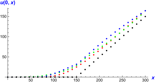
Figure 1: Black-Scholes solution $u(0,x)$ for different values of the weights.

The self-similar Black-Scholes model generates an exotic pricing for different values of $\mu_{1}$, including the classical one for $\mu_{1}=\displaystyle\frac{1}{2}$.

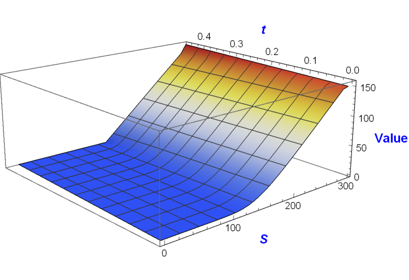
$\mu_{1}=\frac{1}{2}$.

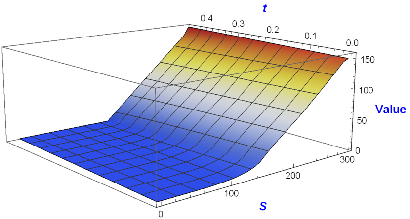
$\mu_{1}=0.2$.

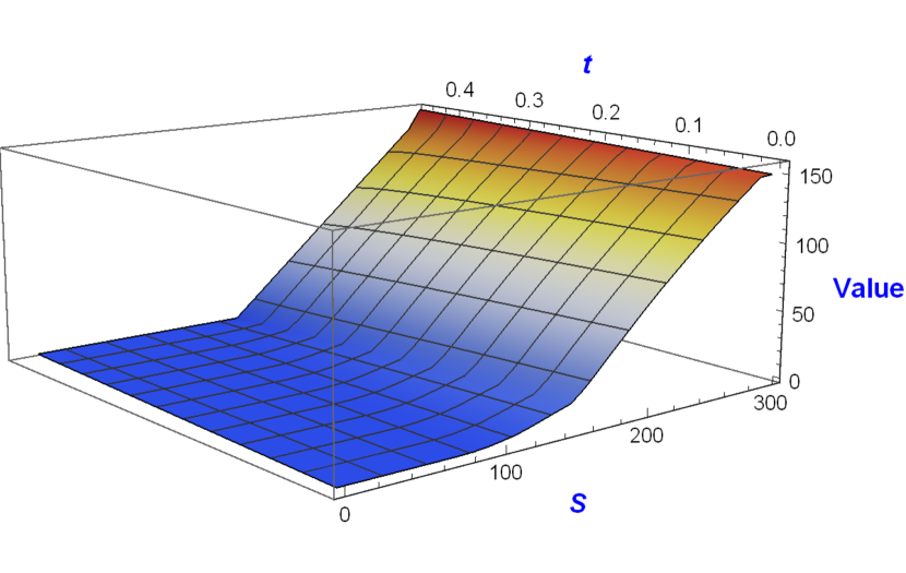
$\mu_{1}=0.8$.

Figure 2: The call value for different values of the weights.

6.4 The Greeks

As in [Dav17], we recall that, in finance, the sensitivity of a portfolio to changes in parameters values can be measured through what commonly call “the Greeks", i.e.,

1. The Delta, $\Delta=\displaystyle\frac{\partial C}{\partial S}\,\in\,[0,1]$, which enables one to quantify the risk, and is thus the most important Greek. It can also be interpreted as a probability that the option will expire in the money.

2. The Gamma, $\Gamma=\displaystyle\frac{\partial^{2}C}{\partial S^{2}}\geqslant 0$, which measures the rate of the acceleration of the option price, with respect to changes in the underlying price.

3. The Vega (the name of which comes from the form of the Greek letter $\nu$), $\nu=\displaystyle\frac{\partial C}{\partial\sigma}$, which measures the sensitivity to volatility.

4. The Theta $\Theta=\displaystyle\frac{\partial C}{\partial t}$, which is the time cost of holding an option.

5. The rho, $\rho=\displaystyle\frac{\partial C}{\partial r}$, which measures the sensitivity to the risk-free interest rate.
   

The good strategy, for traders, is to have delta-neutral positions at least once a day, and, whenever the opportunity arises, to improve the Gamma and the Vega.

6.4.1 The Delta

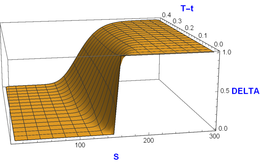
$\mu_{1}=\frac{1}{2}$.

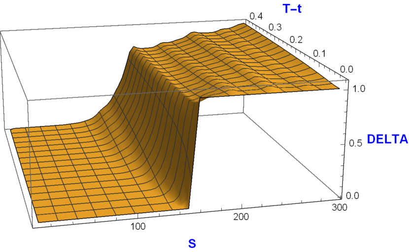
$\mu_{1}=\frac{1}{3}$.

$\mu_{1}=\frac{2}{3}$.

Figure 3: The $\Delta$, for different values of the weights.

6.4.2 The Gamma

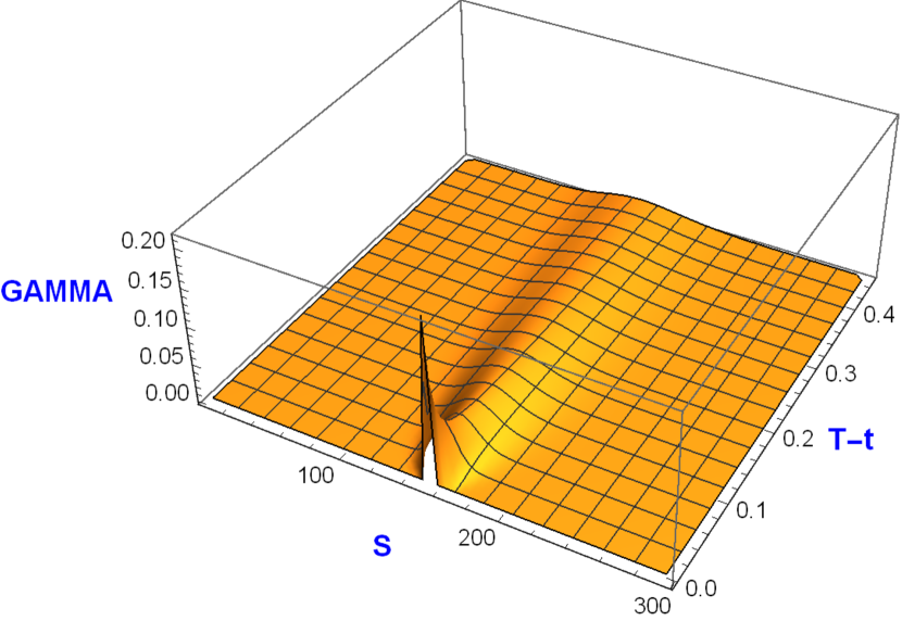
$\mu_{1}=\frac{1}{2}$.

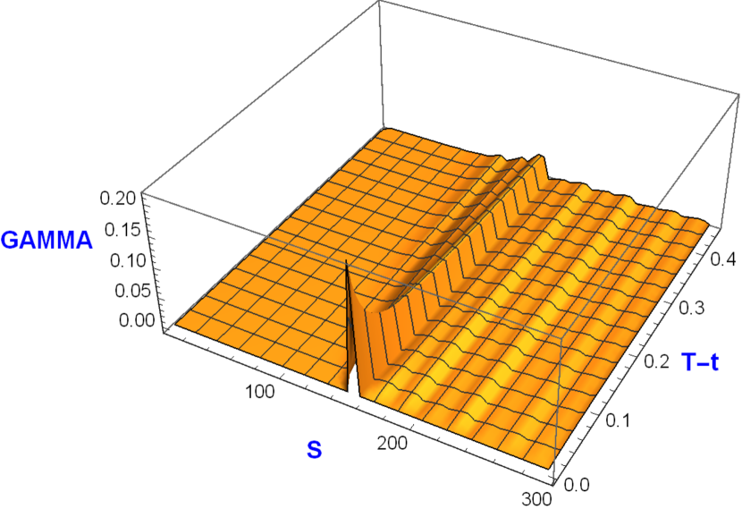
$\mu_{1}=\frac{1}{3}$.

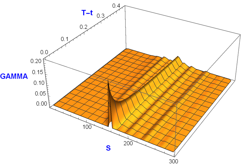
$\mu_{1}=\frac{2}{3}$.

Figure 4: The $\Gamma$, for different values of the weights.

6.4.3 The Theta

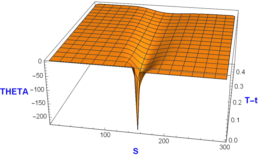
$\mu_{1}=\frac{1}{2}$.

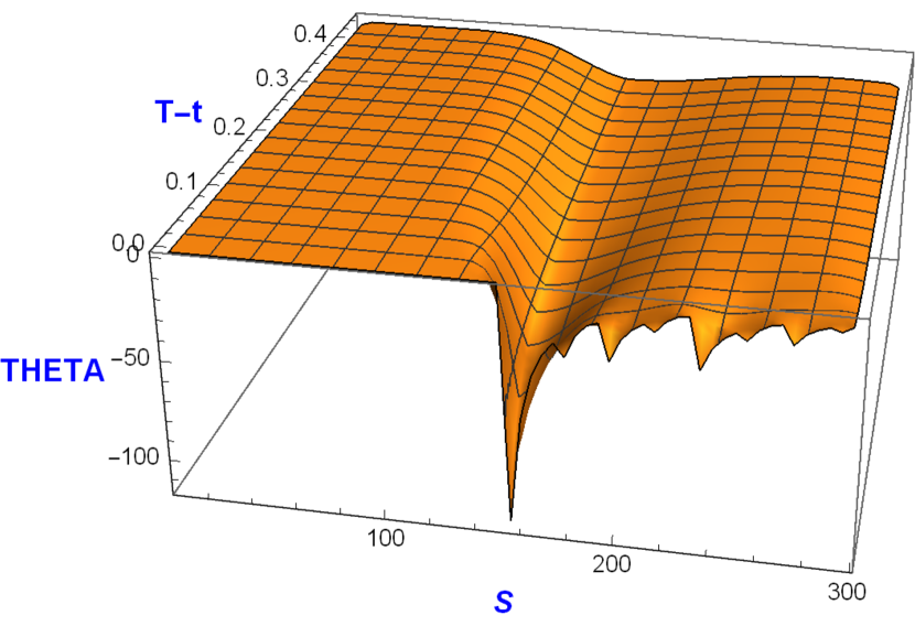
$\mu_{1}=\frac{1}{3}$.

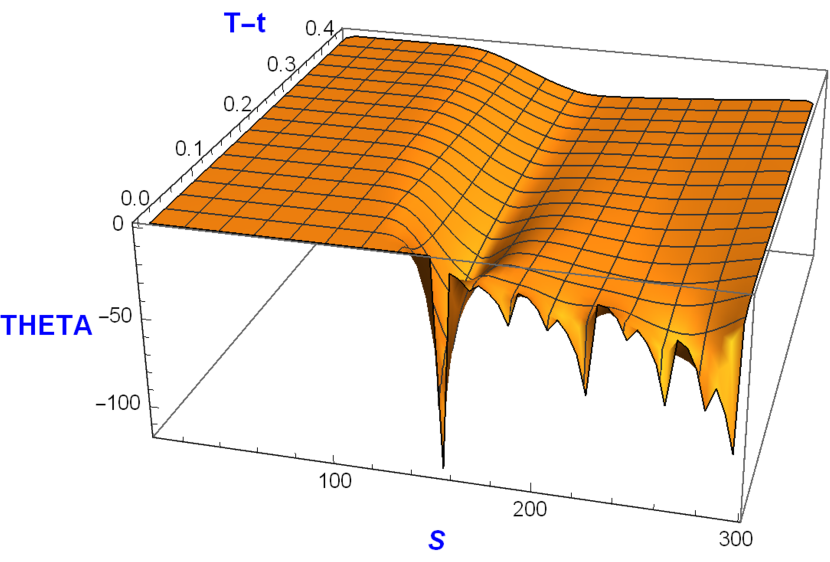
$\mu_{1}=\frac{2}{3}$.

Figure 5: The $\Theta$, for different values of the weights.

6.4.4 The Vega

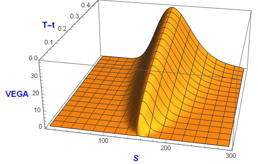
$\mu_{1}=\frac{1}{2}$.

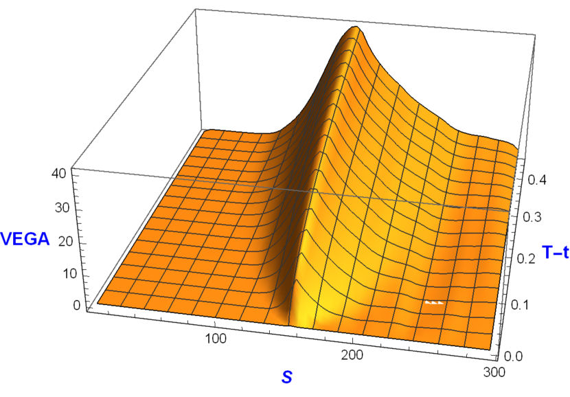
$\mu_{1}=\frac{1}{3}$.

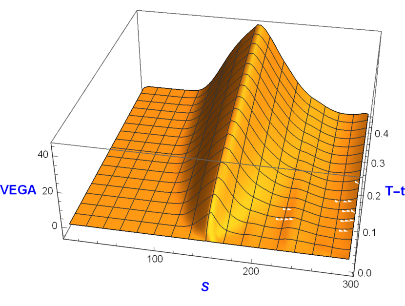
$\mu_{1}=\frac{2}{3}$.

Figure 6: The $\nu$, for different values of the weights.

6.4.5 The rho

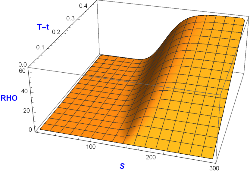
$\mu_{1}=\frac{1}{2}$.

$\mu_{1}=\frac{1}{3}$.

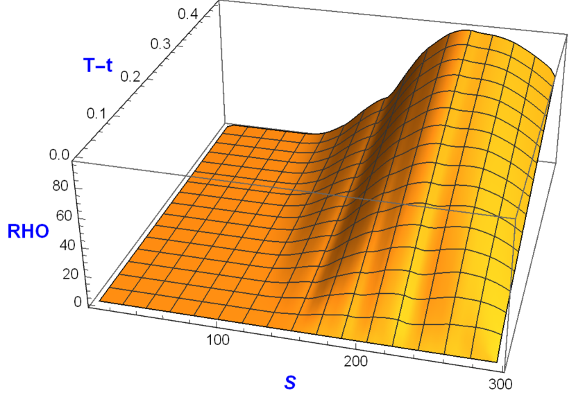
$\mu_{1}=\frac{2}{3}$.

Figure 7: The $\rho$, for different values of the weights.

6.5 Discussion

Let us make a few remarks about the behavior of the solution with respect to the weight $\mu$ at $t=0$:

1. For $\displaystyle\mu_{1}=\frac{1}{3}$: the premium is greater than that of the classical model under the strike and smaller above. The Greeks value shows a drastic increase in the strike neighbor, and self-similarity clearly affects in the money region. The Theta shows a slower premium expected decrease.
   

2. For $\displaystyle\mu_{1}=\frac{2}{3}$: the premium is everywhere greater than that of the classical model. The Greeks value increases progressively in the strike neighbor, and self-similarity affects in the money region. The Theta indicates a slower premium expected decrease in the money and a greater decrease deep in the money.
   

The dynamic generated by the self-similar Black-Scholes model is exotic and enables the emergence of non-standard behaviors, the parameter $\displaystyle\mu_{1}$ can capture the behavior of non confident investors under uncertainty and other factors influencing their perception of future.

The self-similar Black-Scholes equation can be understood as a diffusion equation with a time change through self-similar probability $\mu$, where the cumulative distribution function satisfies for $x\in\left]0,1\right[$, $\left[0,x\right]=f_{\mathcal{W}}(\left[0,1\right])$ for some word $\mathcal{W}$,

$$\mu\left[0,x\right] =\Pi_{i\in\mathcal{W}}\,\mu_{i}$$

depending on the address (path) of $x$. According to this remark, we can create more exotic behavior by using a self-similar measure $\mu$ with many weights or enable the weights to change over time.

References

- [AP05] Y. Achdou and O. Pironneau. Computational Methods for Option Pricing. Society for Industrial and Applied Mathematics, 2005.
- [Dav17] C. David. Control of the Black-Scholes equation. Comput. Math. Appl., 73(7):1566–1575, 2017.
- [For96] P. Fortune. Anomalies in option pricing: The black-scholes model revisited. New England Economic Review, March/April:17–40, 1996.
- [HLN06] J. Hu, K.-S. Lau, and S.-M. Ngai. Laplace operators related to self-similar measures on . Journal of Functional Analysis, 239:542–565, 2006.
- [Kig01] J. Kigami. Analysis on Fractals. Cambridge University Press, 2001.
- [Kil94] T. Kilpeläinen. Weighted sobolev spaces and capacity. Annales Academiae Scientiarum Fennicae. Series A I. Mathematica, 19(1):95–113, 1994.
- [KN01] R. Kangro and R. Nicolaides. Far field boundary conditions for black-scholes equations. SIAM Journal on Numerical Analysis, 38(4):1357–1368, 2001.
- [LM68] J.-L. Lions and E. Magenes. Problèmes aux limites non homogènes et applications. Dunod, 1968.
- [LMM05] G. C. Lim, G. M. Martin, and V. L. Martin. Parametric pricing of higher order moments in s&p500 options. Journal of Applied Econometrics, 20(3):377–404, 2005.
- [Man97] B. B. Mandelbrot. Fractals and Scaling in Finance. Springer New York, 1997.
- [MR92] Z.-M. Ma and M. Röckner. Introduction to the Theory of (Non-Symmetric) Dirichlet Forms. Springer-Verlag, 1992.
- [RD19] N. Riane and C. David. The finite difference method for the heat equation on sierpiński simplices. International Journal of Computer Mathematics, 96(7):1477–1501, 2019.
- [RD21] N. Riane and C. David. An inverse black–scholes problem. Optimization and Engineering, 22:2183–2204, 2021.
- [Str06] R. S. Strichartz. Differential Equations on Fractals. A Tutorial. Princeton University Press, 2006.
- [Wlo87] J. Wloka. Partial differential equations. Cambridge University Press, 1987.
- [Zei90] E. Zeidler. Nonlinear Functional Analysis and its Applications. II/A.: Linear Monotone Operators. Springer, 1990.