Quantum Circuit for High Order Perturbation Theory Corrections
Abstract
Perturbation theory (PT) might be one of the most powerful and fruitful tools for both physicists and chemists, which has led to a wide variety of applications. Over the past decades, advances in quantum computing provide opportunities for alternatives to classical methods. Recently, a general quantum circuit estimating the low order PT corrections has been proposed. In this article, we revisit the quantum circuits for PT calculations, and develop the methods for higher order PT corrections of eigenenergy, especially the \nth3 and \nth4 order corrections. We present the feasible quantum circuit to estimate each term in these PT corrections. There are two the fundamental operations in the proposed circuit. One approximates the perturbation terms, the other approximates the inverse of unperturbed energy difference. The proposed method can be generalized to higher order PT corrections.
Introduction
In the recent decades, quantum computing has attracted enormous interests for the potential quantum speedup[1, 2, 3]. The scope of its applications have been incrementally broadened into a variety of fields, ranging from prime factorization[4, 5, 6, 7] to data classification[8, 9, 10, 11]. Among these applications, estimating the eigenenergy of many-body systems might be one of the most promising applications of quantum computing[12, 13, 14, 15, 16, 1, 17, 18]. In this context, a branch of approaches has been employed to solve the classically intractable electronic structure problems, such as the powerful variational quantum eigensolver[19, 20, 21], quantum Monte Carlo simulations[22, 23, 24, 25], and the flexible variational quantum simulator[26, 27].
In our recent work[28], we have proposed a general quantum circuit for Perturbation theory (PT) calculations. Perturbation theory (PT) might be one of the most powerful and fruitful tools for both physicists and chemists, which is a powerful tool to approximate solutions to intricate eigenenergy problems. In 1926[29], Schrödinger’s proposed the first important application of time-independent PT for quantum systems to obtain quantum eigenenergy. In our recent work[28], we have proposed a general quantum circuit estimating the low order PT corrections: the first order correction for eigenstate, the first and the second order corrections for energy. The proposed quantum circuit shows potential speedup comparing to the classical PT calculations when estimating second order energy corrections. Even though, it still remains an open question whether the propose method can be generalized to higher order PT corrections. In some cases higher order PT corrections are in demand, especially when approximating the accurate energy levels of a complicated system. One example is Møller–Plesset perturbation theory (MPPT)[30], which is a typical and powerful PT method in computational chemistry, where the high order corrections are often critical for accurate approximation of molecules.
To address these issues, here we present a general approach to estimate these high order PT corrections of energy, especially for the \nth3 and \nth4 order PT corrections of energy. The proposed method is also feasible for the higher order ones.
Before diving deep, hereafter the time-independent PT method is revisited briefly, which is often termed as Rayleigh–Schrödinger PT. In the time-independent PT method, the Hamiltonian of a complicated unsolved system is described as
| (1) |
represents the unperturbed Hamiltonian, represents the perturbation and . is often a simple and solvable system, and we have , where and are the eigenstates and corresponding energy levels of . Time-independent PT method leads to the following approximation[31]
where indicate the -th order correction of energy, and indicate the -th order correction of eigenstate. The order and order energy corrections are given as
| (2) |
and
| (3) |
where all terms involved are summed over , and we introduce the following notations for simplicity
Main
Estimate the \nth3 order PT correction of energy
In Eq.(2), there are two summations in the third order PT correction of energy . For simplicity, we denote the first summation in over as For the order PT correction (), the first term is defined as
| (4) |
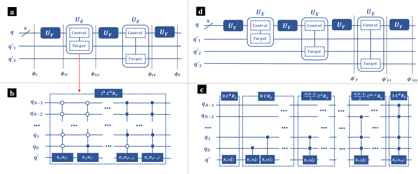
In Fig.(1a) a schematic diagram of the quantum circuit estimating is presented. Register are qubits that represent the given system, whereas are ancilla qubits introduced to implement summations. There are in total qubits, indicating that there are at maximum energy levels, where it is assumed that there is no degeneracy. Initially, all qubits are prepared at state , and qubits are prepared at state , which is the state in the computational basis. Rigorously, state should be written as , where is the binary form of with digits, and each digit corresponds to a qubit. For simplicity, in this article we always use notation instead of . In the following discussion, we denote the quantum states at certain steps as , corresponding to the stages noted by the dashed lines in Fig.(1a,d). After the initialization, we have the overall quantum state as
| (5) |
where subscripts indicate the corresponding registers.
Next, operation is applied on the qubits, which approximates the perturbation . Generally the perturbation term is not unitary, which can not be directly simulated on a quantum computer. Alternatively, here we approximate the perturbation term with , which can be simulated with Trotter decomposition[32, 33]. Thus, can be given as
| (6) |
where is a unitary transformation that converts the eigenstate sets into the corresponding computational basis , . More information of can be found in Methods section. Eq.(6) guarantees that
| (7) |
After applying , the overall quantum state is
| (8) |
We then apply operator to estimate the inverse of . acts on both and qubits, where all are control qubits and the single qubit is target. is defined as
| (9) |
where is defined in Eq.(20). generates the inverse of with
| (10) |
where is a real constant ensuring that . Intuitively, can be decomposed into gates, where all of the qubits are control qubits and is the target. In our recent work[28], we have presented an improved implementation of , which is as depicted in Fig.(1c). In the improved design, there are still multi-controlled gates, but only one of them is gate. Briefly, there are gates, and the angles are defined as Eq.(22). More details about are presented in the Methods section. The detailed implementation of and can be found in our recent work[10, 28].
converts the overall quantum state as
| (11) |
In our recent work[10], we have demonstrated that the first order correction of eigenstate can be obtained from , as is approximated by . Here our aim is the higher order corrections, and the succeeding operations are still required. Next, is once again applied on the qubits, and then is applied on and , where qubits are still the control qubits but is the target. The new overall quantum state is
| (12) |
Afterwards, is applied on qubits for the third time, and we have the overall quantum circuit is
| (13) |
where the subscript of indicates that it acts on qubits. By the end, all qubits are measured. Theoretically, the probability to get result is
| (14) |
By this mean , the first term of , can be estimated.
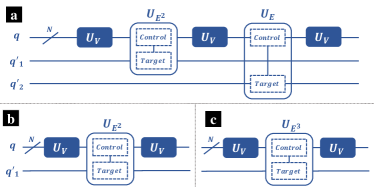
In the second term of , is already obtained as the first order correction of energy. Moreover, can be estimated by the quantum circuit as shown in Fig.(2b), where the is the operation estimating the inverse of .
Estimate the \nth4 order PT correction of energy
There are four terms in the the \nth4 order PT correction . For simplicity, we denote the first summation in over as . Similarly to , can be estimated by the quantum circuit as shown in Fig.(1d), where and are still harnessed to approximate the perturbations and the inverse of . In addition to the qubits and the ancilla qubits , , there is one new ancilla qubit noted as . To avoid confusions, here we denote the overall quantum states in Fig.(1d) at certain stage as . At beginning, all qubits are initialized at state , whereas all of the ancilla qubits are prepared at the ground state . The circuit before is exactly the same quantum circuit that estimates , as depicted in Fig.(1a). Therefore, we have
| (15) |
Next, is applied on and , where are the control qubits and is the target. The overall quantum state is
| (16) |
where for simplicity, we only present the terms that contribute to the estimation of . Then is applied on the qubits, and we have . At the end, all of the qubits are measured. The probability to get result is
| (17) |
Then consider the second term in . Notice that the summations over and are separable. is already estimated in , and is the second order correction . Thus, the second term in is known as long as the lower order corrections have been obtained. The third term in , can be estimated by the quantum circuit as shown in Fig.(2a), where estimates the inverse of . As for the last term of , is already known, and can be estimated by the quantum circuit as shown in Fig.(2c), where the is the operation estimating the inverse of , which estimates the inverse of .
Discussion
In this section we will discuss the time complexity of the proposed quantum circuits. For simplicity, we denote as the total number of unperturbed energy levels, and there are in total qubits. Recalling the quantum circuits estimating as depicted in Fig.(1a), is applied twice and is applied three times. In the quantum circuits estimating as depicted in Fig.(1d), is applied three times and is applied four times. acts on the qubits, whereas acts on both the and qubits. Generally, the multi controller gates in consumes more time than the Trotter decomposition in . A gate can be decomposed into basic gates[34]. On the other hand, to prepare a single term with Trotter decomposition, no more than basic gates are necessary[33]. Thus, often denominates the overall time complexity[10, 28].
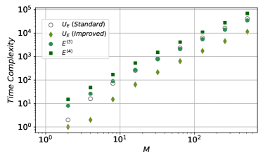
In the standard design of as depicted in Fig.(1b), there are gates in total, which can be decomposed into basic gates. The total time complexity of the improved design of as shown in Fig.(1c) is[28],
Time complexity of and is exactly the same to . Similarly, and denominate the time complexity of the quantum circuits that estimate the miscellaneous terms as shown in Fig.(2).
In Fig.(3), we present the overall time complexity of , along with the overall time complexity of quantum circuits that estimate , against , the total number of energy levels. Time complexity of the standard design of , as shown in Fig.(1b), is depicted with the hollowed circles, whereas the diamonds corresponds to the time complexity of the improved design of as shown in Fig.(1c). We can find out that the improved consumes much less time than the standard one. Moreover, we also depicted the overall time consuming to estimate , , corresponding to the octagons and squares, where the improved is applied. For great , we find out that the time complexity of denominates the overall time consuming to estimate , .
In higher order PT corrections, the terms can still be described by Eq.(4), where superscript indicates the order correction. Our approach estimating , can be generalized to higher order terms , with deeper circuit and more ancilla qubits. Generally, each in the denominator corresponds to a acting on and an ancilla digit . On the other hand, each in the numerator corresponds to a acting on the qubits. Thus, to estimate in the order correction, ancilla qubits are necessary, and will be applied on the qubits for times, whereas will be repeat for times.
Conclusions
In this article, we revisit the quantum circuits for PT calculations, and propose a general quantum circuit to estimate the higher order PT corrections of eigenenergy, especially the \nth3 and \nth4 order corrections. To estimate the PT energy corrections on a quantum computer, the fundamental task is to approximate , which describes the perturbation, and , which is the difference between unperturbed energy levels. In this context, and are introduced to estimate these crucial components. In the proposed quantum circuit, and are applied for several times to estimate the intricate summations in the PT corrections. We also discuss the time complexity of the proposed quantum circuits. Generally, denominates the overall time complexity. Our work smooths the way to implement high order PT calculations, and PT-based methods on with a quantum computer.
Data availability
All data that support the plots within this paper and other findings of this study are available from the corresponding author upon reasonable request.
Acknowledgement
J.L gratefully acknowledges funding by National Natural Science Foundation of China (NSFC) under Grant No.12305012.
Author contributions
J.L. and X.G. discussed the results and wrote the main manuscript text.
Competing interests
The authors declare no competing interests.
Methods
More details about the transformation
In PT the unperturbed Hamiltonian is solvable, and thus can be diagonalized as
| (18) |
There exists an transformation denoted as , which converts the eigenstate sets into the computational basis , . Then we have
| (19) |
is often well-developed for the typical many-body systems. As an instance, the transformation that diagonalize the dynamics of strongly correlated quantum systems can be implemented with Bogoliubov transformation and quantum Fourier transformation[35]
More details about
For the standard as depicted in Fig.(1b), we have
| (20) |
where is the same constant in Eq.(10). The improved implementation of can be written as,
| (21) |
where is an integer corresponds to the unperturbed energy level, and is the digit in the corresponding binary form of . Constraints to the values can be written as
| (22) |
where is the same integer in Eq.(21), and the set is
| (23) |
, are digits in the binary forms of , . and share the similar structure of . In and , in Eq.(20,22) are replaced as and .
References
- [1] John Preskill. Quantum computing in the nisq era and beyond. Quantum, 2:79, 2018.
- [2] Yudong Cao, Jonathan Romero, Jonathan P Olson, Matthias Degroote, Peter D Johnson, Mária Kieferová, Ian D Kivlichan, Tim Menke, Borja Peropadre, Nicolas PD Sawaya, et al. Quantum chemistry in the age of quantum computing. Chemical reviews, 119(19):10856–10915, 2019.
- [3] Manas Sajjan, Junxu Li, Raja Selvarajan, Shree Hari Sureshbabu, Sumit Suresh Kale, Rishabh Gupta, Vinit Singh, and Sabre Kais. Quantum machine learning for chemistry and physics. Chemical Society Reviews, 2022.
- [4] Peter W Shor. Algorithms for quantum computation: discrete logarithms and factoring. In Proceedings 35th annual symposium on foundations of computer science, pages 124–134. Ieee, 1994.
- [5] Matthew Hayward. Quantum computing and shor’s algorithm. Sydney: Macquarie University Mathematics Department, 1, 2008.
- [6] Ben P Lanyon, Till J Weinhold, Nathan K Langford, Marco Barbieri, Daniel FV James, Alexei Gilchrist, and Andrew G White. Experimental demonstration of a compiled version of shor’s algorithm with quantum entanglement. Physical Review Letters, 99(25):250505, 2007.
- [7] Thomas Monz, Daniel Nigg, Esteban A Martinez, Matthias F Brandl, Philipp Schindler, Richard Rines, Shannon X Wang, Isaac L Chuang, and Rainer Blatt. Realization of a scalable shor algorithm. Science, 351(6277):1068–1070, 2016.
- [8] Maria Schuld, Ilya Sinayskiy, and Francesco Petruccione. Quantum computing for pattern classification. In PRICAI 2014: Trends in Artificial Intelligence: 13th Pacific Rim International Conference on Artificial Intelligence, Gold Coast, QLD, Australia, December 1-5, 2014. Proceedings 13, pages 208–220. Springer, 2014.
- [9] Sonika Johri, Shantanu Debnath, Avinash Mocherla, Alexandros Singk, Anupam Prakash, Jungsang Kim, and Iordanis Kerenidis. Nearest centroid classification on a trapped ion quantum computer. npj Quantum Information, 7(1):122, 2021.
- [10] Junxu Li and Sabre Kais. Quantum cluster algorithm for data classification. Materials Theory, 5:1–14, 2021.
- [11] Johannes Herrmann, Sergi Masot Llima, Ants Remm, Petr Zapletal, Nathan A McMahon, Colin Scarato, François Swiadek, Christian Kraglund Andersen, Christoph Hellings, Sebastian Krinner, et al. Realizing quantum convolutional neural networks on a superconducting quantum processor to recognize quantum phases. Nature Communications, 13(1):4144, 2022.
- [12] Alán Aspuru-Guzik, Anthony D Dutoi, Peter J Love, and Martin Head-Gordon. Simulated quantum computation of molecular energies. Science, 309(5741):1704–1707, 2005.
- [13] Hefeng Wang, Sabre Kais, Alán Aspuru-Guzik, and Mark R Hoffmann. Quantum algorithm for obtaining the energy spectrum of molecular systems. Physical Chemistry Chemical Physics, 10(35):5388–5393, 2008.
- [14] Benjamin P Lanyon, James D Whitfield, Geoff G Gillett, Michael E Goggin, Marcelo P Almeida, Ivan Kassal, Jacob D Biamonte, Masoud Mohseni, Ben J Powell, Marco Barbieri, et al. Towards quantum chemistry on a quantum computer. Nature chemistry, 2(2):106–111, 2010.
- [15] Rongxin Xia and Sabre Kais. Quantum machine learning for electronic structure calculations. Nature communications, 9(1):4195, 2018.
- [16] Sam McArdle, Suguru Endo, Alán Aspuru-Guzik, Simon C Benjamin, and Xiao Yuan. Quantum computational chemistry. Reviews of Modern Physics, 92(1):015003, 2020.
- [17] Xiao Mi, Matteo Ippoliti, Chris Quintana, Ami Greene, Zijun Chen, Jonathan Gross, Frank Arute, Kunal Arya, Juan Atalaya, Ryan Babbush, et al. Time-crystalline eigenstate order on a quantum processor. Nature, 601(7894):531–536, 2022.
- [18] Seunghoon Lee, Joonho Lee, Huanchen Zhai, Yu Tong, Alexander M Dalzell, Ashutosh Kumar, Phillip Helms, Johnnie Gray, Zhi-Hao Cui, Wenyuan Liu, et al. Evaluating the evidence for exponential quantum advantage in ground-state quantum chemistry. Nature Communications, 14(1):1952, 2023.
- [19] Alberto Peruzzo, Jarrod McClean, Peter Shadbolt, Man-Hong Yung, Xiao-Qi Zhou, Peter J Love, Alán Aspuru-Guzik, and Jeremy L O’brien. A variational eigenvalue solver on a photonic quantum processor. Nature communications, 5(1):4213, 2014.
- [20] Jarrod R McClean, Jonathan Romero, Ryan Babbush, and Alán Aspuru-Guzik. The theory of variational hybrid quantum-classical algorithms. New Journal of Physics, 18(2):023023, 2016.
- [21] Google AI Quantum, Collaborators*†, Frank Arute, Kunal Arya, Ryan Babbush, Dave Bacon, Joseph C Bardin, Rami Barends, Sergio Boixo, Michael Broughton, Bob B Buckley, et al. Hartree-fock on a superconducting qubit quantum computer. Science, 369(6507):1084–1089, 2020.
- [22] WMC Foulkes, Lubos Mitas, RJ Needs, and Guna Rajagopal. Quantum monte carlo simulations of solids. Reviews of Modern Physics, 73(1):33, 2001.
- [23] M Peter Nightingale and Cyrus J Umrigar. Quantum Monte Carlo methods in physics and chemistry. Number 525. Springer Science & Business Media, 1998.
- [24] Masuo Suzuki. Quantum Monte Carlo methods in condensed matter physics. World scientific, 1993.
- [25] Sergey Bravyi, Anirban Chowdhury, David Gosset, and Pawel Wocjan. Quantum hamiltonian complexity in thermal equilibrium. Nature Physics, 18(11):1367–1370, 2022.
- [26] Ying Li and Simon C Benjamin. Efficient variational quantum simulator incorporating active error minimization. Physical Review X, 7(2):021050, 2017.
- [27] Suguru Endo, Jinzhao Sun, Ying Li, Simon C Benjamin, and Xiao Yuan. Variational quantum simulation of general processes. Physical Review Letters, 125(1):010501, 2020.
- [28] Junxu Li, Barbara A Jones, and Sabre Kais. Toward perturbation theory methods on a quantum computer. Science Advances, 9(19):eadg4576, 2023.
- [29] Erwin Schrödinger. An undulatory theory of the mechanics of atoms and molecules. Physical review, 28(6):1049, 1926.
- [30] Chr Møller and Milton S Plesset. Note on an approximation treatment for many-electron systems. Physical review, 46(7):618, 1934.
- [31] David J Griffiths and Darrell F Schroeter. Introduction to quantum mechanics. Cambridge university press, 2018.
- [32] Seth Lloyd. Universal quantum simulators. Science, 273(5278):1073–1078, 1996.
- [33] James D Whitfield, Jacob Biamonte, and Alán Aspuru-Guzik. Simulation of electronic structure hamiltonians using quantum computers. Molecular Physics, 109(5):735–750, 2011.
- [34] Adriano Barenco, Charles H Bennett, Richard Cleve, David P DiVincenzo, Norman Margolus, Peter Shor, Tycho Sleator, John A Smolin, and Harald Weinfurter. Elementary gates for quantum computation. Physical review A, 52(5):3457, 1995.
- [35] Frank Verstraete, J Ignacio Cirac, and José I Latorre. Quantum circuits for strongly correlated quantum systems. Physical Review A, 79(3):032316, 2009.