Context-dependent Causality
(the Non-Monotonic Case)

Abstract

We develop a novel identification strategy as well as a new estimator for context-dependent causal inference in non-parametric triangular models with non-separable disturbances. Departing from the common practice, our analysis does not rely on the strict monotonicity assumption. Our key contribution lies in leveraging on diffusion models to formulate the structural equations as a system evolving from noise accumulation to account for the influence of the latent context (confounder) variable on the outcome. Our identifiability strategy involves a system of Fredholm integral equations expressing the distributional relationship between a latent context variable and a vector of observables. These integral equations involve an unknown kernel and are governed by a set of structural form functions, inducing a non-monotonic inverse problem. We prove that if the kernel density can be represented as an infinite mixture of Gaussians, then there exists a unique solution for the unknown function. This is a significant result, as it shows that it is possible to solve a non-monotonic inverse problem even when the kernel is unknown. On the methodological front we leverage on a novel and enriched Contaminated Generative Adversarial (Neural) Networks (CONGAN) which we provide as a solution to the non-monotonic inverse problem.

Keywords: Counterfactual; Diffusion; Synthetic distribution; Unrestricted support; Contaminated Generative Adversarial Networks; Context; Non-monotonic inverse problem; Unknown kernel function; Neural Networks; Fredholm integral equation

1 Introduction

Consequences are propagated by actions taken in a specific and often latent contextual platform. As such, context is an intrinsic part of a causal model, playing the role of unobserved heterogeneity. The common practice in the treatment of unobserved heterogeneity is to impose various kinds of structural form restrictions on the relationships among actions and consequences. A widely used structural restriction is the monotonicity assumption, which implies a one-to-one relationship between either the action or the outcome variable and its random disturbance (given the control variables). A key limitation of this assumption however, is that it rules out any source of uncertainty regarding the unobservables when the observables are held fixed. Namely, monotonicity forces a degenerate conditional distribution of the unobservables given the observables. Consequently, the theoretical model is restricted to a subset of structural form functions and thus, may poorly identify and capture the true underlying causal relationship between action and outcome.

We depart from the conventional reliance on monotonicity to achieve identifiability. Yet, we keep the general architecture similar to the conventional modeling. The present model is a nonparametric triangular model with non-separable disturbances, which includes a latent context variable. Context is modeled as a confounder with unobserved heterogeneity given the observables, challenging the conventional causal inference. The main challenge in achieving identifiability is aggravated due to the absence of an adjustment set (observed control variables) to be conditioned on in order to satisfy some conditional independence assumption. This identifiability relies on formulating the structural equations as a system evolving from noise accumulation, known as a diffusion process to account for the influence of the latent context (confounder) on the outcome. This allows us to achieve identifiability without the limitations of monotonicity assumptions. The key result of the offered identifiability approach introduced here importantly emanates from the fact that any possible set of structural functions belonging to an equivalence class of triangular models generating the data yields the same do-interventional counterfactual distribution. This result is achieved by expressing the distributional relationship between a latent context variable and a vector of observables through a system of Fredholm integral equations. The aforementioned set of equations is governed by the set of generator functions and an unknown kernel function, inducing a non-monotonic inverse problem. The role of these generator functions is two-fold: (i) to characterize an admissible kernel function induced by these generator functions and (ii) to ensure that the estimator of the unknown quantity is a continuous function of the data for any given kernel function in the equivalence class. We establish that the interventional distribution is invariant to the choice of the kernel if it belongs to any strongly complete family of densities, e.g., an infinite mixture of Gaussians. This is a significant result, as it shows that it is possible to solve a non-monotonic inverse problem even when the kernel is unknown.

The framework offered is general and may have a significant impact on a wide variety of economic and other phenomena inclusive of those intrinsically exhibiting non-monotonicity in their confounding variables. The relationship between the equivalence class of structural form functions and the causal distribution is formed by the establishment of a newly introduced augmented Fourier series expansion. This novel expansion method is designed to characterize an infinite system of linear regression equations satisfying cross-equation restrictions, induced by an equivalence class of non-separable structural form functions. These cross-equation restrictions are derived from the common triangular model assumptions, without reliance on any variant of monotonicity.

The existing literature using either local average treatment effects or triangular models architecture impose various functional form restrictions, such as conditional quantile restrictions (Chesher, 2003), strict monotonicity in the case of average local treatment effects (Imbens  Angrist, 1994) as well as in the case of triangular models (Imbens  Newey, 2009; Hoderlein ., 2017). Alternative models assume restricted support domain (locality) (Hoderlein  Mammen, 2009; Angrist ., 1996; Altonji  Matzkin, 2005; Heckman  Vytlacil, 2005). These restrictions guarantee the identifiability of the latent confounder up to a strictly monotonic transformation from conditional quantiles of the observables. The main limitation of such treatment however, is to potentially narrow down the support domain of the latent space. This can be detrimental to causal inference as it eliminates a subset of the control (placebo) group, when employing e.g., the common practice of partial means (Newey, 1994), interventions (Pearl, 2019) and local average treatment effect (Angrist ., 1996). Monotonicity is rather not an innocuous restriction as it is at odds with many phenomena in general and those in economics in particular. The potential bias propagated by relying on the monotonicity assumption has long been estimated, (e.g., Klein (2010)). However, there is a lack of alternative identifiability, inference and an appropriate estimator which are not monotonicity-based. Monotonicity is a strong and perhaps unpalatable for many basic economic phenomena such as demand, supply and consumption behaviour (Hoderlein ., 2016; Hoderlein  Mammen, 2007), multiple equilibria in strategic behavior (Myerson, 1999), search behavior (Chetverikov, 2019; Agarwal ., 2020) as well as in prospect theory (Kahneman  Tversky, 1979).

In our present framework, we depart from the above mentioned restrictions by allowing for the posterior distribution of the latent context to be a function of the covariates and of the outcome. This generalization incorporates cases in which the context is also a function of the outcome and not only the covariates, unlike the control variable approach (Mammen ., 2012; Mammen ., 2016; Chernozhukov ., 2020, to mention a few). The presence of a latent context covariate affects the cause and the outcome simultaneously and thus, is the source of endogeneity in our model. Thus, the endogeneity can be eliminated by allocating each one of the cause and outcome a different and independent realization of the context. Building upon this idea, we develop a novel identification strategy as well as a new estimator for triangular models in the presence of non-separable disturbances. Unlike the common practice, our approach does not rely on the strict monotonicity assumption, but rather on an integral equation characterized by generator functions. These generator functions induce an equivalence class of triangular models, while exploiting the entire support domain of the latent space in a non-monotonic manner. This insight solves the double-hurdle problem of relying on monotonicity as well as on a restricted support domain (Chernozhukov ., 2020) which may produce inferior results as is shown in our simulations.

The new paradigm presented here yields a synthetic counterfactual distribution, which is entropy-advantageous. We provide a novel feed-forward multi-layer Neural network-based estimator. This is performed by leveraging on a novel extension namely, a Contaminated version we develop and apply to the Generative Adversarial Networks model (CONGAN) (Goodfellow ., 2014). The advantage of the proposed practice is that it enables the Neural network to be trained on the entire support domain of the latent space unlike the common practice, which uncovers counterfactual relationships by averaging available observable data on a restricted support.

The paper proceeds as follows. Section 2 gives an overview of the common practice of causal inference in triangular models. Section 3 presents the diffusion problem formulation and its underlying assumptions. Section 4 shows an alternative formulation of the triangular model as an integral equation to simplify the analysis. Section 5 provides an illustrative example for identifiability which does not rely on monotonicity assumption. Section 6 characterizes strong completeness of sufficient statistic as a building block for identifiability. Section 7 presents the identifiability by relying on strong completeness. The estimator is presented in section 8. In section 9 Monte-Carlo simulations are used to verify our theoretical model performance. Section 10 concludes.

2 Discussion and literature review

Various identification strategies have been designed to uncover counterfactual relationships in triangular models, consisting of non-additively separable disturbances, in the absence of experimental data. The ultimate goal of these approaches is to mimic a “natural experiment” (Rosenzweig  Wolpin, 2000) by detaching a random variable $X$ (an observed action or treatment) from the unobservables affecting some other random variable $Y$ (outcome). The prominent question they answer is what would have been the expected counterfactual outcome of $Y$ if the values of the independent variable $X$ were assigned independently of the disturbances. Generally, in order to achieve this goal, monotonicity is imposed either on the unobservables in the first stage regression (Imbens  Newey, 2009; Blundell  Matzkin, 2014; Heckman  Robb, 1985; Hoderlein  Mammen, 2009; Chernozhukov ., 2020, to mention a few); or on the unobservables in the outcome’s structural equation in the second stage (Chernozhukov ., 2007; Kim, 2020). In other cases, the monotonicity requirement is imposed on the instrumental variable (Imbens  Angrist, 1994; Hoderlein ., 2017; Heckman  Pinto, 2018). However, this assumption is at odds with many actual phenomena as discussed earlier. Moreover and perhaps more importantly, it imposes severe limitations on the set of identifiable causal relationships in nonparametric inference, while potentially missing the true causal relationship. The unattended issue in the existing literature is that the direction and strength of causal relationship is context-blind.

An alternative identifiability strategy for causal inference not relying on monotonicity is obtained by assuming ignorability which is known also as an unconfoundedness assumption (Athey  Imbens, 2016) or a conditional independence on observables (Farrell ., 2021). This approach limits the scope of causal analysis by requiring a directly observed set of control variables, which are rarely available in reality, in order to introduce conditional independence. The present study departs from this approach by embracing a generative covariate mechanism (Mammen ., 2012, 2016) producing a synthetic sample of the same distribution present in the data. This approach does not necessitate the unconfoundedness assumption, yet allows for the estimation of the counterfactual distribution at any level of accuracy desired (given amount of data available and level of complexity). This methodology also departs from the popular quantile structural estimation, which is intrinsically monotonic (Chernozhukov ., 2013).

We contribute to the existing literature in two specific aspects. The theoretical contribution amounts to developing a new causal identification paradigm, which is non-parametric, monotonicity-free, context-dependent and universal with respect to the identifiable function set. Our new paradigm yields a counterfactual distribution exploiting the unrestricted support domain of the latent space, which is essential for the practice of intervention and counterfactual inference. On the methodological front, we develop a novel estimation strategy referred to here as a Contaminated Generative Adversarial Networks (CONGAN). This approach consists of two generators and one classifier: counterfactual samples generator and a contaminator generator. The classifier determines whether the sample is real or synthetic as in the conventional GAN (Goodfellow ., 2014). The main difference is in the unique role of each one of the generators in the causal inference. The counterfactual samples generator intends to mimic the causal relationship between $X$ and $Y$, which would be the case if $X$ and the unobservables were distributionally independent. However, it cannot be trained directly using the observed data, in which $X$ and the latent context variable are distributionally jointly dependent. Consequently, the role of the contaminator is to minimize the disparity between the observed and the counterfactual samples. As such, the contaminator is a nuisance Neural network which is essential for training the counterfactual generator. Our new paradigm enables to mimic the distribution of $Y$ given $X$ that would have been obtained under random assignment of the latent context variable (independently of $X$). We emphasize at this stage that context is not just a semantic concept but rather an identifiability instrument, in that it permits rendering $Y$ a different contextual regime from the one governing $X$. Once the regime governing $Y$ does not longer comove with $X$, one mimics the effect of an exogenous variation in $X$ on $Y$. The benefit of the contaminated Neural network is in that it precludes the need to invert the generators in order to account for the posterior distribution of the latent context variable given the observables, which is computationally cumbersome. Our CONGAN application utilizes multi-layer feed-forward Neural networks in which, unlike in other series estimators (e.g., sieve), the basis functions themselves are data-driven by combining simple functions. Such a flexible combination is known to be capable of approximating any measurable function to any desired degree of accuracy (Hornik ., 1989). In the ensuing section we attend to the theoretical triangular model formulation.

3 Diffusion-based non-monotonic triangular models

Consider the following triangular simultaneous equations model, pioneered by Heckman  Robb (1985). The model includes three observed random variables $X,Y,Z\in\mathbb{R}$, and two unobserved random disturbances $\upeta\in\mathbb{R}$ and $\bm{\epsilon}:=(\epsilon_{1},...,\epsilon_{d})\in\upchi^{d}\subset\mathbb{R}^{d}$. The triplet $(Z,\bm{\epsilon},\upeta)$ generates a pair of observed quantities $X,Y\in\mathbb{R}$, as an infinite Gaussian mixtures governed by unknown location as well as variance functional parameters $(\mu_{1,i},\mu_{2,i})$ and $(\sigma_{1,i},\sigma_{2,i})$. There are unknown mixing proportion parameters $(\alpha_{1,i},\alpha_{2,i})$. Let $L$ be the number of components in the Gaussian mixtures of $(X,Y)$, which approaches infinity, depicted as,

$$X=h(z,\eta)\sim\sum_{i=1}^{L}\alpha_{1,i}\mathcal{N}\left(\mu_{1,i}(z)+\rho_{12}\sigma_{1,i}(z)\left(\frac{\eta-\mu_{\eta}}{\sigma_{\eta}}\right),\sigma_{1,i}^{2}(z)(1-\rho_{i,12}^{2})\right)$$ (1)

and $Y=g(X,\upepsilon)$ satisfying,

$$g(X,\upepsilon)|\upeta=\eta\sim\sum_{i=1}^{L}\alpha_{2,i}\mathcal{N}\left(\mu_{2,i}(X)+\rho_{i,13}(X)\sigma_{2,i}(X)\left(\frac{\eta-\mu_{\eta}}{\sigma_{\eta}}\right),\sigma_{2,i}^{2}(X)(1-\rho_{i,13}^{2}(X))\right).$$ (2)

The random variable $Y$ is the outcome variable, whereas $X$ represents an action or an endogeneous variable. The random variable $Z$ is an exogenous covariate also known as an instrumental variable. The random variable $Z$ is assumed to be continuous with an unknown density $f_{Z}(z)$, and is further assumed to satisfy $Z\mathchoice{\mathrel{\hbox to0.0pt{$\displaystyle\perp$\hss}\mkern 2.0mu{\displaystyle\perp}}}{\mathrel{\hbox to0.0pt{$\textstyle\perp$\hss}\mkern 2.0mu{\textstyle\perp}}}{\mathrel{\hbox to0.0pt{$\scriptstyle\perp$\hss}\mkern 2.0mu{\scriptstyle\perp}}}{\mathrel{\hbox to0.0pt{$\scriptscriptstyle\perp$\hss}\mkern 2.0mu{\scriptscriptstyle\perp}}}(\upeta,\bm{\epsilon})$. The disturbances $(\upeta,\bm{\epsilon})$ are assumed to be continuous and possibly jointly dependent. We denote their unknown joint and marginal distributions by $F_{\upeta,\bm{\epsilon}}$, $F_{\upeta}$ and $F_{\bm{\epsilon}}$, respectively.

Equivalently, the Gaussian Cholesky decomposition parameterized by the functional parameters $\left\{\upbeta_{i}\right\}$ with $\upbeta_{i}(x):=\rho_{i,13}^{2}(x)$ and a constant $\uptheta_{i}:=\rho_{12}^{2}$ can be used to simplify the analytical formula of the data Gaussian mixture data generation process in Eqs. (1) and (2),

$$X=\sum_{i=1}^{L}\alpha_{1,i}\left\{\mu_{1,i}(Z)+\sigma_{1,i}(Z)\left(\sqrt{1-\uptheta_{i}}\Phi^{-1}(\bm{\nu}_{i,x})+\sqrt{\uptheta_{i}}\left(\frac{\upeta-\mu_{\eta}}{\sigma_{\eta}}\right)\right)\right\},$$

$$Y=\sum_{i=1}^{L}\alpha_{2,i}\left\{\mu_{2,i}(X)+\sigma_{2,i}(X)\left(\sqrt{1-\upbeta_{i}(X)}\Phi^{-1}(\bm{\nu}_{i})+\sqrt{\upbeta_{i}(X)}\left(\frac{\upeta-\mu_{\eta}}{\sigma_{\eta}}\right)\right)\right\},$$

with independent uniformly distributed random variables $\bm{\upnu}_{i}$ and $\bm{\upnu}_{i,x}$. We define $\alpha_{i,j}^{*}:=\alpha_{1,i}\alpha_{2,j}$ to express the observed outcome as a function of $(X,Z)$,

$$Y=\sum_{\begin{subarray}{c}i,j=1\end{subarray}}^{L}\alpha_{i,j}^{*}\left\{\mu_{2,i}(X)+\sigma_{2,i}(X)\left(\sqrt{1-\upbeta_{i}(X)}\Phi^{-1}(\bm{\nu}_{i})+\sqrt{\upbeta_{i}(X)}\left(\frac{\Psi_{j}(X,Z)+\bm{\epsilon}_{0}-\mu_{\eta}}{\sigma_{\eta}}\right)\right)\right\},$$ (3)

where $\Psi_{j}(X,Z)$ for any given noise $\bm{\epsilon}_{0}$ is just a one of the infinite potential values of $\upeta$ in the $j$’th component of the mixture for any given $(X,Z)$. Eq. (3) is a reduced-form representation of $Y$ without any endogenous predictor variables. This formulation shares similarities with diffusion models (Ho ., 2020) by capturing the influence of noise on $Y$.

We attend to the following definition of the support of a continuous random vector $Q$ in $\mathbb{Q}^{n}$ with a probability density function $f_{Q}$,

Definition 3.1 (Support).

$\text{Supp}(Q):=\text{The closure of the set of points for which }f_{Q}(q)\neq 0$.

We consider a non-parametric setting, whereby the unknown function $h$ is assumed to be continuous, but otherwise of general structural form. The unknown function $g$ can be continuous or piecewise constant, in the latter case leading to a discrete outcome $Y$. As in Imbens  Newey (2009) the functions $h$ and $g$ may be nonseparable in their respective disturbances $\upeta$ and $\bm{\epsilon}$. The model (1)-(2) implies that $\upeta$ is a confounder or common cause, affecting both $X$ directly via (1), and $Y$ indirectly through the dependence of $\bm{\epsilon}$ on $\upeta$. Finally, following previous work (Imbens  Newey, 2009), we assume the following standard condition holds:

Assumption 3.1 (Common support).

The conditional random variable $\upeta|X=x$ has a fixed support independent of $x$. Namely, $\text{Supp}(\upeta|X=x)=\text{Supp}(\upeta),$ $\forall x$.

For future use, we present two important properties of the above triangular model. First, note that Eq. (1) together with the assumption that $Z$ is independent of $(\upeta,\bm{\epsilon})$ imply that $X\mathchoice{\mathrel{\hbox to0.0pt{$\displaystyle\perp$\hss}\mkern 2.0mu{\displaystyle\perp}}}{\mathrel{\hbox to0.0pt{$\textstyle\perp$\hss}\mkern 2.0mu{\textstyle\perp}}}{\mathrel{\hbox to0.0pt{$\scriptstyle\perp$\hss}\mkern 2.0mu{\scriptstyle\perp}}}{\mathrel{\hbox to0.0pt{$\scriptscriptstyle\perp$\hss}\mkern 2.0mu{\scriptscriptstyle\perp}}}\bm{\epsilon}|\upeta$. The second property is stated in the following auxiliary lemma (see proof in appendix E).

Lemma 3.1.

Under assumption 3.1 it holds that,

$$\text{Supp}(\left.\bm{\epsilon}\right|X=x)=\text{Supp}(\bm{\epsilon})\quad\forall x\in\text{Supp}(X).$$ (4)

Given $n$ i.i.d. triplets $(x_{i},y_{i},z_{i})$ from the above triangular model, Eqs. (1)-(2), the goal is to estimate the counterfactual distribution of the outcome $Y$ if $X$ were set to the value $x$. Depending on the particular application, this quantity is related to policy effect or treatment effect. In the notation of causal inference (Pearl, 2019), the above quantity of interest is known as intervention. It is given by

$$T(y|x)=P\left(Y\leq y|\text{do}(X=x)\right):=\mathbb{E}_{\bm{\epsilon}\sim F_{\bm{\epsilon}}}\left[\mathds{1}\left\{g(x,\bm{\epsilon})\leq y\right\}\right].$$ (5)

It is worth emphasizing that under the above triangular model and its assumptions, even exact knowledge of the joint distribution of $(X,Y,Z)$ does not uniquely determine the quantity $T(y|x)$ (Imbens, 2007). The reason is that even if $g$ were known, under (1)-(2) the random variables $X$ and $\bm{\epsilon}$ might be jointly dependent. In contrast, in Eq. (5) the expectation is over the marginal distribution of $\bm{\epsilon}$, effectively treating $\bm{\epsilon}$ as independent of $X$.

To guarantee identifiability of $T(y|x)$, several previous works imposed an additional assumption of strict monotonicity of $h(z,\eta)$ in the second argument $\eta$, required to hold for all $z$ in its support, e.g., Blundell  Matzkin (2014); Imbens  Newey (2009). Specifically, Imbens  Newey (2009) defined the following random variable $V:=F_{X|Z}(X)$ and the following functional, both of which can be estimated from the observed data,

$$H_{c}(y|x)=\int_{0}^{1}F_{Y|X=x,V=v}(y)dv.$$ (6)

The strict monotonicity assumption implies that the random variable $V$ is a one-to-one mapping of the unobserved disturbance $\upeta$. Furthermore, it can be shown that $V$ is a control variable and that $H_{c}(y|x)=T(y|x)$. Then, an estimate of $H_{c}$ directly yields an estimate of $T(y|x)$.

The identifiability strategy described above is based on the ability to uniquely determine $\upeta$, up to a strictly monotonic transformation, for any pair of observed $(X,Z)$. As we now describe, we significantly depart from this approach. Instead, we leverage on the known axiom of continuity and building block of expected utility theory and post the following assumption:

Assumption 3.2 (Continuity of $X|Z$ and $\bm{\epsilon}|\upeta$).

Assumption 3.2.a.

For any $z\in\text{Supp}(Z)$, the random variable $X|Z=z$ is continuous. In particular, the set of values of $\upeta$ where $\partial h(z,\eta)/\partial\eta=0$ is of measure zero.

Assumption 3.2.b.

The random vector $\bm{\epsilon}|\upeta$ is a $d$-dimensional continuous random vector for any $\upeta$.

Assumption 3.3 (Completeness).

The distribution of the random vector $(X,\upeta)|Z$ belongs to a complete family of distributions with respect to $Z$.

Assumption 3.4 (Square integrability).

The density $f(y|X=x,Z=z)$ is square integrable, and is known.

The first key contribution of our work is to show that under the triangular model with assumptions 3.1-3.4, the intervention $T(y|x)$ is identifiable. Consequently, the fact that additive and monotonic triangular models are identifiable, are special cases of our more general identifiability result (Imbens, 2007; Imbens  Newey, 2009; Blundell  Matzkin, 2014; Heckman  Robb, 1985).

We establish identifiability in a population setting, where assume to have observed an infinite number of triplets $(x_{i},y_{i},z_{i})$ from the triangular model (1)-(2). Hence, in what follows we assume that the joint distribution $F_{X,Y,Z}$ as well as various conditional distributions, such as $F_{Y|X=x,Z=z}$ are all perfectly known. Our approach to prove identifiability proceeds as follows. First, in Section A, we derive an integral equation relating the intervention of Eq. (5) to known distributions of $(X,Y,Z)$. In general, there may be an infinite number of solutions to this integral equation, which reflects the fact that in the original triangular model, the unknown functions $h$ and $g$ are not identifiable. Yet, in Section 7 we prove that any solution of this integral equation gives the same intervention, hence proving identifiability of the intervention.

4 An alternative representation for the intervention

A key preliminary step is to derive an alternative representation for the intervention $T(y|x)$. Consider the following cumulative distribution function (CDF),

$$H(y|x)=\mathbb{E}_{\upeta}[F_{Y|X=x,\upeta}(y)]=\int F_{Y|X=x,\upeta=\eta}(y)f_{\upeta}(\eta)d\eta.$$ (7)

Note that the function inside the integral , with $\upeta$ attaining all possible values in its support, is well defined by assumption 3.1. The following lemma is key to our proposed approach, both for proving identifiability and for inference.

Lemma 4.1 (Functional equivalence).

Under the triangular model with assumption 3.1, the function $H(y|x)$ defined in Eq. (7) satisfies that $\forall\hskip 1.99997pt(x,y)$ in the relevant support,

$$H(y|x)=T(y|x).$$ (8)

Proof.

Using the definition of $Y$ in Eq. (2) the function $F_{Y|X=x,\upeta}(y)$ may be equivalently written as follows

$$F_{Y|X=x,\upeta}(y)=\mathbb{E}_{\bm{\epsilon}|X=x,\upeta}\left[\mathds{1}\left\{Y\leq y\right\}|X=x,\upeta\right]=\mathbb{E}_{\bm{\epsilon}|X=x,\upeta}\left[\mathds{1}\left\{g(x,\bm{\epsilon})<y\right\}\right].$$ (9)

By conditional independence $X\mathchoice{\mathrel{\hbox to0.0pt{$\displaystyle\perp$\hss}\mkern 2.0mu{\displaystyle\perp}}}{\mathrel{\hbox to0.0pt{$\textstyle\perp$\hss}\mkern 2.0mu{\textstyle\perp}}}{\mathrel{\hbox to0.0pt{$\scriptstyle\perp$\hss}\mkern 2.0mu{\scriptstyle\perp}}}{\mathrel{\hbox to0.0pt{$\scriptscriptstyle\perp$\hss}\mkern 2.0mu{\scriptscriptstyle\perp}}}\epsilon|\upeta$, the random vector $\bm{\epsilon}|X=x,\upeta$ has the same distribution as $\bm{\epsilon}|\upeta$. Inserting the resulting expression back into Eq. (7) gives that

$$H(y|x)=\mathbb{E}_{\upeta\sim F_{\upeta}}\left[\mathbb{E}_{\bm{\epsilon}|\upeta}\left[\mathds{1}\left\{g(x,\bm{\epsilon})\leq y\right\}\right]\right].$$ (10)

By the law of total expectation, the RHS is simply $\mathbb{E}_{\bm{\epsilon}}[\mathds{1}\left\{g(x,\bm{\epsilon})\leq y\right\}]$, which by Eq. (5) is $T(y|x)$. ∎

By Lemma 4.1, instead of estimating $T(y|x)$ which involves a $d$-dimensional integration over $\bm{\epsilon}$, one may instead estimate the function $H(y|x)$ that depends on a univariate integral w.r.t. $\upeta$. The specific expectation operator in Eq. (7) is known as the partial means estimator (Newey, 1994), since the expectation is taken w.r.t. the unconditional distribution $F_{\upeta}$ rather than the conditional one $F_{\upeta|X=x}$. As such, $H(y|x)$ is a counterfactual distribution.

5 An Example for a Triangular Data Generation Process

Let’s examine the non-monotonic case, $h(z,\eta)\neq F_{X|Z=z}^{-1}(F_{\upeta}(\eta))$.

$$\bm{\Sigma}_{y,\eta}(X,Z):=\left[\begin{matrix}\sigma_{y}^{2}(X)&\sigma_{2}(x)\sigma_{\eta}(X,Z)\rho_{13}(X)\\ \sigma_{2}(x)\sigma_{\eta}(X,Z)\rho_{13}(X)&\sigma_{\eta}^{2}(X,Z)\end{matrix}\right]$$

The coefficient $\rho_{13}(x)$ determines the conditional correlation between $Y$ and $\upeta$ given $X=x,Z=z$.

$$Z\sim F_{Z},\quad\upeta\sim N(\mu_{\eta},\sigma_{\eta}^{2})$$

$$X|Z=z,\upeta=\eta\sim N\left(\mu_{1}(z)+\rho_{12}\sigma_{1}(z)\left(\frac{\eta-\mu_{\eta}}{\sigma_{\eta}}\right),\sigma_{x}^{2}(z)(1-\rho_{12}^{2})\right)$$

$$Y|X=x,Z=z\sim N\left(\mu_{2}(x)+\rho_{13}(x)\sigma_{2}(x)\left(\frac{\eta(x,z)-\mu_{\eta}}{\sigma_{\eta}}\right),\sigma_{y}^{2}(x)(1-\rho_{13}^{2}(x))\right)$$

Recall that $\upeta\mathchoice{\mathrel{\hbox to0.0pt{$\displaystyle\perp$\hss}\mkern 2.0mu{\displaystyle\perp}}}{\mathrel{\hbox to0.0pt{$\textstyle\perp$\hss}\mkern 2.0mu{\textstyle\perp}}}{\mathrel{\hbox to0.0pt{$\scriptstyle\perp$\hss}\mkern 2.0mu{\scriptstyle\perp}}}{\mathrel{\hbox to0.0pt{$\scriptscriptstyle\perp$\hss}\mkern 2.0mu{\scriptscriptstyle\perp}}}Z$. Yet, $\upeta\not\mathchoice{\mathrel{\hbox to0.0pt{$\displaystyle\perp$\hss}\mkern 2.0mu{\displaystyle\perp}}}{\mathrel{\hbox to0.0pt{$\textstyle\perp$\hss}\mkern 2.0mu{\textstyle\perp}}}{\mathrel{\hbox to0.0pt{$\scriptstyle\perp$\hss}\mkern 2.0mu{\scriptstyle\perp}}}{\mathrel{\hbox to0.0pt{$\scriptscriptstyle\perp$\hss}\mkern 2.0mu{\scriptscriptstyle\perp}}}Z|X$. Similarly, $Y\mathchoice{\mathrel{\hbox to0.0pt{$\displaystyle\perp$\hss}\mkern 2.0mu{\displaystyle\perp}}}{\mathrel{\hbox to0.0pt{$\textstyle\perp$\hss}\mkern 2.0mu{\textstyle\perp}}}{\mathrel{\hbox to0.0pt{$\scriptstyle\perp$\hss}\mkern 2.0mu{\scriptstyle\perp}}}{\mathrel{\hbox to0.0pt{$\scriptscriptstyle\perp$\hss}\mkern 2.0mu{\scriptscriptstyle\perp}}}Z|X,\upeta$. In the equation of $X$, each value of $Z$ characterizes a specific conditional Gaussian (given $\upeta$). In the equation of $Y$, each value of $X$ characterizes a specific conditional Gaussian (given $\upeta$). We employ Gaussian Cholesky decomposition to simplify the analytical formula of the data generation process,

$$X(z,\eta,\bm{\varepsilon}_{x})=\mu_{1}(z)-\rho_{12}\sigma_{1}(z)\frac{\mu_{\eta}}{\sigma_{\eta}}+\sigma_{1}(z)\rho_{12}\frac{\upeta}{\sigma_{\eta}}+\sigma_{1}(z)\sqrt{1-\rho_{12}^{2}}\Phi^{-1}(\bm{\varepsilon}_{x})$$

$$Y(x,z,\bm{\nu})=\mu_{2}(x)-\rho_{13}(x)\sigma_{2}(x)\frac{\mu_{\eta}}{\sigma_{\eta}}+\sigma_{2}(x)\rho_{13}(x)\frac{\upeta(z,x)}{\sigma_{\eta}}+\sigma_{2}(x)\sqrt{1-\rho_{13}^{2}(x)}\Phi^{-1}(\bm{\nu})$$ (11)

$$\upeta\frac{\sigma_{1}(z)\rho_{12}}{\sigma_{\eta}}=x-\mu_{1}(z)+\rho_{12}\sigma_{1}(z)\frac{\mu_{\eta}}{\sigma_{\eta}}-\sigma_{1}(z)\sqrt{1-\rho_{12}^{2}}\Phi^{-1}(\bm{\varepsilon}_{x})$$

$$\upeta=\mu_{\eta}+\frac{\sigma_{\eta}}{\sigma_{1}(z)\rho_{12}}(x-\mu_{1}(z))-\frac{\sigma_{\eta}\sqrt{1-\rho_{12}^{2}}}{\rho_{12}}\Phi^{-1}(\bm{\varepsilon}_{x})$$

$$\sigma_{\eta}(x,z):=\frac{\sigma_{\eta}\sqrt{1-\rho_{12}^{2}}}{\rho_{12}}$$

$$\mu_{\eta}(x,z):=\mu_{\eta}+\frac{\sigma_{\eta}}{\sigma_{1}(z)\rho_{12}}\left(x-\mu_{1}(z)\right)\quad\mu_{\eta}=0\quad(\text{a normalization})$$

$$\upeta(z,x)=\mu_{\eta}(x,z)-\sigma_{\eta}(x,z)\Phi^{-1}(\bm{\varepsilon}_{x}).$$

where $\upeta(x,z):=\upeta|X=x,Z=z\sim N\left(\mu_{\eta}(x,z),\sigma_{\eta}^{2}(x,z)\right)$. The unknown parameters characterizing the latent confounder $\upeta$ are: $(\rho_{12},\rho_{13}(\cdot),\mu_{\eta},\sigma_{\eta})$. The rest of the parameters can be directly measured from the joint distribution of the observables $(X,Y,Z)$.

Identifying $\rho_{12}$ from the covariance with observable.

$$\mathbb{E}_{\upeta}\left[\mathbb{COV}\left[X,Z\right]|\upeta\right]=\mathbb{COV}\left[\mu_{1}(z),Z\right]+\sqrt{1-\rho_{12}^{2}}\mathbb{COV}\left[\sigma_{1}(z)\Phi^{-1}(\bm{\varepsilon}_{x}),Z\right]$$

This gives,

$$\sqrt{1-\rho_{12}^{2}}=\frac{\mathbb{COV}\left[X,Z\right]-\mathbb{COV}\left[\mu_{1}(z),Z\right]}{\mathbb{COV}\left[\sigma_{1}(z)\Phi^{-1}(\bm{\varepsilon}_{x}),Z\right]}$$

Given $\rho_{12}$, the coefficient $\rho_{13}(x)$ can be identified by a linear regression of the form,

$$Y(x,z,\bm{\nu})=\overbrace{\mu_{2}(x)}^{\mathbb{E}[Y|X=x]}-\rho_{13}(x)\left[\frac{\sigma_{2}(x)}{\sigma_{1}(z)\rho_{12}}\overbrace{(x-\mu_{1}(z))}^{x-\mathbb{E}[X|Z=z]}\right]+\epsilon$$

The counterfactual outcome variable

$$Y^{\text{CF}}(\text{Do}(X=x))=\mu_{2}(x)+\rho_{13}(x)\sigma_{2}(x)\left(\frac{\eta-\mu_{\eta}}{\sigma_{\eta}}\right)+\sigma_{2}(x)\sqrt{1-\rho_{13}^{2}(x)}\Phi^{-1}(\bm{\nu})$$ (12)

Define $\upbeta:=\rho_{13}^{2}(x)$. For any given pair $(x,z)$, $Y$ can be reconstructed from a noise propagated by $\bm{\nu}$,

$$Y(x,z)=\mu_{2}(x)+\sqrt{\upbeta}\sigma_{2}(x)\left(\frac{\eta(x,z)-\mu_{\eta}}{\sigma_{\eta}}\right)+\sigma_{2}(x)\sqrt{1-\upbeta}\Phi^{-1}(\bm{\nu}).$$ (13)

The non-contaminated output is defined as follows,

$$Y_{0}:=\Phi^{-1}(\bm{\nu}).$$

The observed output is a contaminated variant of $Y_{0}$ is known as a diffusion process (Ho ., 2020),

$$\frac{Y(x,z)-\mu_{2}(x)}{\sigma_{2}(x)}:=\sqrt{1-\upbeta}Y_{0}+\sqrt{\upbeta}\left(\frac{\eta(x,z)-\mu_{\eta}}{\sigma_{\eta}}\right).$$ (14)

It can be seen that the posterior distribution of $\eta$ given $x$ and $z$ does not play any role in $Y_{0}$. In the present diffusion model we only need to recover the parameters $(\mu_{2}(x),\sigma_{2}(x))$ characterizing $Y(x,z)$ for any give pair $(x,z)$. This requires to identify the nuisance parameters $\beta$ and $\rho_{12}$ as depicted above. Eq. (12) gives us the direct linkage between the identified parameters and the counterfactual output. Namely, by substituting $\eta(x,z)$ in Eq. (14) with a random draw from the prior distribution of $\upeta$ we get a counterfactual sample from $Y^{\text{CF}}$.

The next building block is formulating a two-regime model describing the relationship among members in a complete family of distributions, facilitating generalizing the identifiability achieved in the simple example above.

6 Completeness of Sufficient Statistic

Definition 6.1 (Completeness).

Let $X$ be a random variable with density functions parameterized by $\theta$. A statistic $T(X)$ is said to be complete if, for every measurable function $g$, the following holds:

$$\mathbb{E}[g(T(X))]=0\text{ for all }\theta\implies g(T(X))=0\text{ almost everywhere.}$$

In simpler terms, if the expected value of any function of the statistic is zero for all possible values of the parameter $\theta$, then the function itself must be almost everywhere equal to zero.

Now, we attend to a stronger variant of completeness, bridging between regimes nested in the same model.

Informal Definition (Strong completeness). The concept of strong completeness applied to the relationship between regimes (subsets of a parameter space), introduced by Alamatsaz (1983), asserts the invariance of expected values of functions with respect to a parameter in some regime (for some fixed setting of the remaining parameters), implying invariance with respect to this parameter in any other regime (other fixed settings of the remaining parameters).

Two Mutually Exclusive Regimes Nested in a Single Model

In the figure above we present a two-regime model parameterized by $(\theta_{1},\theta_{2})$ belonging to a strongly complete family of distributions with respect to $\theta_{1}$. Under strong completeness, family of regime $B$ (each member is a different realization of $\Theta_{1}$) is informative for policy makers that want to infer about family of regime $A$ because these two families share a common parameter space $\theta_{1}$. We next attend to a formal definition of strong completeness.

Definition 6.2 (Strong Completeness).

A family of distributions $F:=\left\{F_{Y|\theta_{1},\theta_{2}}:\theta_{1}\in\Theta_{1}\right\}$ parameterized by $(\theta_{1},\theta_{2})$ of $d$-dimensional random vectors is said to be strongly complete with respect to $\theta_{1}$, if for every function $m:\mathbb{R}^{d}\to\mathbb{R}$ satisfying,

$$\mathbb{E}_{Y\sim F_{Y|\theta_{1},\theta_{2}}}\left[m(\bm{Y})\right]=0\quad\forall\theta_{1}\in\Theta_{1},$$

we have that,

$$\mathbb{E}_{Y\sim F_{Y|\theta_{1},\theta_{2}}}\left[\mathds{1}\left\{m(\bm{Y})=0\right\}\right]=1\quad\forall(\theta_{1},\theta_{2})\in\Theta_{1}\times\Theta_{2}.$$

Consequently, in the presence of a model related to a strongly complete family of distributions with respect to common parameters $\theta_{1}\in\Theta_{1}$, invariance to these common parameters in one regime $\theta_{2}=\theta_{2}^{\prime\prime}$ holds also in the rest of regimes $\theta_{2}^{\prime}\in\Theta_{2}$. This enables to inform policy decisions in different real-world settings (regime $A$).

7 Identifiability

In this section we prove the identifiability of the intervention $T(y|x)$. This is done in two steps. First, we alleviate the issue of the triangular model dependence on multiple unknown quantities. The most prominent one being the dependence of the disturbances on the endogenous covariate. This is implemented by employing an equivalent representation for the structural functions (lemmas 7.1 and 7.2 to follow) in a canonical form, which is invariant to the specification of the unknown quantities (joint-distribution of the disturbances). Second, we use canonical form representation to characterize an equivalence class of normalized-triangular models and establish that identifiability is universal in that it holds for any structural continuous function in the equivalence class (theorem 7.2).

7.1 Normalized triangular models via error-decoupling mechanism

In what follows, ${X}^{*}\overset{d}{=}X$ indicates that the two random variables $X^{*}$ and $X$ have the same distribution. Using this notation, the triangular model is reformulated via an error-decoupling mechanism with disturbances that are uniformly distributed. To this end, given random variables $\upomega$ and $\nu_{1},\ldots,\nu_{d}$, define the following transformed random variables,

$$\Lambda_{0}=\Lambda_{0}(\upomega):=F_{\upeta}^{-1}(\upomega),$$ (15)

and recursively for $1\leq j\leq d$,

$$\Lambda_{j}=\Lambda_{j}(\upomega,\nu_{1},...,\nu_{j}):=F_{\epsilon_{j}|(\Lambda_{0}(\upomega),\Lambda_{1}(\upomega,\nu_{1}),\ldots,\Lambda_{j-1}(\upomega,\nu_{1},\ldots,\nu_{j-1}))}^{-1}(\nu_{j}).$$ (16)

The notations in Eqs. (15)-(16) are used to perform error-decoupling in the following lemma (see proof in appendix E):

Lemma 7.1.

(Error-decoupling) Let $\upomega\sim U[0,1]$ and $\bm{\nu}:=(\nu_{1},\ldots,\nu_{d})\sim U[0,1]^{d}$ be independent of $\upomega$. Consider the following triangular model, where $\Lambda_{0}$ and $\Lambda_{j}$ are defined in Eqs. (15) and (16),

$$X^{*} = h^{*}(Z,\upomega):=h\left(Z,\Lambda_{0}(\upomega)\right),$$ (17)

$$Y^{*} = g^{*}(X^{*},\upomega,\bm{\nu}):=g\left(X^{*},\Lambda_{1}(\upomega,\nu_{1}),\ldots,\Lambda_{d}(\upomega,\nu_{1},\ldots,\nu_{d})\right).$$ (18)

Then, $(X^{*},Y^{*},Z)\overset{d}{=}(X,Y,Z)$.

There are two major differences between the normalized triangular model Eqs. (17)-(18) and the original Eqs. (1)-(2). The first difference is that the disturbances $\upomega$ and $\bm{\nu}$ are independent and in fact uniformly distributed. The second difference, or the price to pay for this decoupling, is that now the disturbance $\omega$ appears explicitly both in the equations for $X$ and for $Y$, namely inside the functions $h^{*}$ and $g^{*}$. Nevertheless, this price is negligible as it alleviates a major challenge in the original triangular model of Eqs. (1)-(2). This challenge stems from the fact that $\upeta$ and $\bm{\epsilon}$ may in general be dependent, in an unknown fashion.

Lemma 7.2 (Normalized Interventional Distribution).

Suppose that assumption 3.2.b holds. Namely, $\bm{\epsilon}|\upeta$ is a $d$-dimensional continuous random vector for any $\upeta$. In terms of the decoupled system as in Eqs. (17)-(18), the quantity of interest (5) admits the following form,

$$H(y|x)=\mathbb{E}_{\begin{subarray}{c}\upomega\sim U[0,1]\\ \bm{\nu}\sim U[0,1]^{d}\end{subarray}}\left[{\mathds{1}\left\{{g^{*}(x,\upomega,\bm{\nu})\leq y}\right\}}\right].$$ (19)

7.2 Identifiability of the interventional distribution

Recall that our primary goal is to estimate the intervention $T(y|x)$ of (5). The key difficulty is that observing $(X,Y,Z)$ does not uniquely determine the functions ${h}^{*}$ and ${g}^{*}$. We alleviate this issue by introducing a set of functions, which are all indistinguishable with respect to the observations. To this end, let $\tilde{F}$ be an arbitrary continuous distribution. Define

$$\widetilde{\mathcal{C}}:=\left\{(\widetilde{h},\widetilde{g}):\widetilde{X}=\widetilde{h}(Z,\widetilde{\upomega}),\,\widetilde{Y}=\widetilde{g}(\widetilde{X},\widetilde{\upomega},\bm{\nu}),\hskip 5.0pt\left(\widetilde{X},\widetilde{Y},Z\right)\overset{d}{=}\left(X^{*},Y^{*},Z\right),\,\widetilde{\upomega}\sim U[0,1],\bm{\nu}\sim U[0,1]^{d}\right\}.$$ (20)

where $\bm{\nu}$ and $\widetilde{\upomega}$ are independent. In other words, the set $\widetilde{\cal C}$ is the equivalence class of the given triangular model. Namely, all pairs of structural functions $\widetilde{h}$ and $\widetilde{g}$ give rise to the same distribution for the observables $(X,Y,Z)$. For any pair $(\tilde{h},\tilde{g})$ there is a corresponding function

$$\tilde{H}(y|x)=\mathbb{E}_{\begin{subarray}{c}\tilde{\upomega}\sim U[0,1]\\ \bm{\nu}\sim U[0,1]^{d}\end{subarray}}\left[{\mathds{1}\left\{{\tilde{g}(x,\tilde{\upomega},\bm{\nu})\leq y}\right\}}\right].$$ (21)

Note that any pair of structural functions $(\widetilde{h},\widetilde{g})\in\mathcal{\widetilde{C}}$ constitutes a distribution,

$$\mathcal{F}_{X,\upomega|Z=z}^{\widetilde{h}}(x,\omega):=\mathbb{E}\left[\mathds{1}\left\{\widetilde{h}(z,\upomega)<x,\upomega<\omega\right\}\right],$$ (22)

as well as a counterfactual distribution,

$$F_{X,Y|Z=z}^{\text{CF}}(x,y):=\mathbb{E}\left[\mathds{1}\left\{\widetilde{h}(z,\upomega)<x,\widetilde{g}(x,\upomega,\bm{\nu})<y\right\}\right],$$

such that the counterfactual density is $f_{X,Y|Z=z}^{\text{CF}}(x,y):=\mathbb{E}\left[\delta(\widetilde{h}(z,\upomega)-x)\delta(\widetilde{g}(x,\upomega,\bm{\nu})-y)\right]$. In next steps, this density of interest is shown to be identifiable.

Lemma 7.3 (Fourier Transform of Counterfactual Density).

Under assumptions 3.1-3.4 the Fourier transform of the counter factual distribution admits the representation as a Fredholm integral equation of the first kind for any pair of frequencies $(\xi_{1},\xi_{2})$ and value of $z$,

$$\Gamma_{\xi_{1},\xi_{2}}(z;(\widetilde{h},\widetilde{g}))=\mathbb{E}_{\begin{subarray}{c}\upomega\sim U[0,1]\\ X\sim F_{X|Z=z}\end{subarray}}\left[\int\exp(-i\xi_{1}\cdot X)\exp(-i\xi_{2}\cdot\widetilde{g}(X,\upomega,\bm{\nu}))d\bm{\nu}\right].$$ (23)

A sufficient condition for identifiability in equivalence class $\mathcal{\widetilde{C}}$ is to uniquely determine the Fourier transform of the counterfactual density from the joint distribution of the triplets $(X,Y,Z)$, namely, having that,

$$\Gamma_{\xi_{1},\xi_{2}}^{\text{CF}}(z;(\widetilde{h},\widetilde{g}))=\Gamma_{\xi_{1},\xi_{2}}^{\text{CF}}(z;(h^{*},g^{*}))\quad\forall(z,\xi_{1},\xi_{2}).$$ (24)

We rely on the following lemma as a building block in establishing that this condition is satisfied under assumptions 3.1-3.4, by formulating the observational equivalence condition in terms of Fourier transform.

Lemma 7.4 (Fourier Transform Coefficients).

Under assumptions 3.1-3.4 the following Fredholm integral equation of the first kind uniformly holds for any pair $(\widetilde{g},\widetilde{h})\in\mathcal{\widetilde{C}}$ constituting a density $\mathcal{F}_{X,\upomega|Z=z}^{h^{*}}(x,\omega))$ as in Eq. (22),

$$\Gamma_{\xi_{1},\xi_{2}}(z)=\mathbb{E}_{(X,\upomega)\sim\mathcal{F}_{X,\upomega|Z=z}^{\widetilde{h}}}\left[\int\exp(-i\xi_{1}\cdot X)\exp(-i\xi_{2}\cdot\widetilde{g}(X,\upomega,\bm{\nu}))d\bm{\nu}\right]\quad\forall(z,\xi_{1},\xi_{2}),$$ (25)

where the LHS is a specific Fourier transform coefficient of the known density $f_{X,Y|Z=z}$ for frequencies $(\xi_{1},\xi_{2})$.

The following theorem 7.1 states that for any two pairs of functions $(g^{*},h^{*})$ and $(\widetilde{g},\widetilde{h})$ satisfying observational equivalence (Eq. (25)), counterfactual equivalence also holds.

Theorem 7.1 (Coefficients comparison).

Let $m(x,y):=\exp(-i\xi_{1}\cdot x)\exp(-i\xi_{2}\cdot y)$. Suppose that the following observational equivalence holds for two mechanisms $(h^{*},g^{*})$ and $(\widetilde{h},\widetilde{g})$ generating $(X^{*},Y^{*})$ and $(\widetilde{X},\widetilde{Y})$, respectively, in regime $\rho\in\left\{0,1\right\}$,

$$\mathbb{E}\left[m(\widetilde{X},\widetilde{Y})|Z=z,\rho=1\right]=\mathbb{E}\left[m(X^{*},Y^{*})|Z=z,\rho=1\right]=\varphi(z)\quad\forall z,$$ (26)

such that, $(X^{*},Y^{*})|Z,\rho$ and $(\widetilde{X},\widetilde{Y})|Z,\rho$ are strongly complete mixtures of Gaussians with respect to $Z$. Then,

$$\mathbb{E}\left[m(\widetilde{X},\widetilde{Y})|Z=z,\rho=0\right]=\mathbb{E}\left[m(X^{*},Y^{*})|Z=z,\rho=0\right]\quad\forall z.$$

This implies that in any regime $\rho$ the conditional expectation of $m(\cdot,\cdot)$ is invariant to the choice of the mechanism.

The theorem below relies on theorem 7.1 to show that Eq. (24) holds. Simply put, it states that the interventional distribution is invariant with respect to the choice of the structural form functions in the equivalence class $\widetilde{\mathcal{C}}$ (see proof in appendix E).

Theorem 7.2 (Identifiability).

Given assumptions 3.1-3.4, the intervention function is uniquely determined from the joint distribution of the triplets $(X,Y,Z)$. Namely, $\forall(\widetilde{g},\widetilde{h})\in\widetilde{\mathcal{C}}$ it holds that,

$$H(y|x)=\tilde{H}(y|x)$$ (27)

The aforementioned may give rise to the following query: can a monotone data generation process produce an equivalent distribution to the one propagated by a non-monotonic data generation process? The answer to such query is definitely negative (as is proven here in lemma .4, Appendix E). This is so because any monotonic data generation process lacks sufficient variation in the distribution of the outcome variable due to the restriction on any value of context producing the same distribution of $Y$ within a fixed conditional quantile of $X$.

So far we have established identifiability for the interventional distribution. This is a very strong result in that it is universal, neither relying on any structural form restrictions nor on any assumptions regarding the true measure (prior to normalization) of the disturbances. Thus, it lends itself to nonparametric treatment. Building on the above identifiability result of the counterfactual distribution, we next develop the synthetic counterfactual machinery. Theorem 7.1 establishes that the kernel can be unknown in Fredholm integral equations, whereas Theorem 7.2 establishes the identifiability of the counterfactual distribution based on the insight of theorem 7.2.

7.3 Synthetic counterfactual machinery

Following theorem 7.2, the interventional distribution $H(y|x)$ is the same for any sequential generator functions in the equivalence class $(h^{*},g^{*})\in\widetilde{\mathcal{C}}$. This result naturally lends itself for an arbitrarily chosen sequential generator functions $(\widetilde{h},\widetilde{g})$ for defining,

$$F_{Y,X|Z=z}^{\text{O}}(y,x|\widetilde{g},\widetilde{h}):=P\left(Y\leq y,X\leq x|Y=\widetilde{g}(X,\upomega,\upnu),X=\widetilde{h}(z,\upomega)\right)$$ (28)

$$=\int_{0}^{1}\int_{[0,1]^{d}}\mathds{1}\left\{\widetilde{g}(\widetilde{h}(z,\omega),\omega,\bm{\nu})\leq y\right\}\mathds{1}\left\{\widetilde{h}(z,\omega)\leq x\right\}d\bm{\nu}d\omega,$$

which is the observed (O) conditional generated density function of $Y$ and $X$ given $Z=z$. Similarly, the observed (O) conditional generated density function of $X$ given $Z=z$ is defined as,

$$F_{X|Z=z}^{\text{O}}(x|\widetilde{h}):=P\left(X\leq x|X=\widetilde{h}(z,\upomega)\right)=\int_{0}^{1}\mathds{1}\left\{\widetilde{h}(z,\omega)\leq x\right\}\hskip 2.5ptd\omega.$$ (29)

Note that the key innovation embedded in (28) is in that the entire support domain $[0,1]\times[0,1]^{d}$ of the latent space (random disturbances) is used to characterize the conditional joint distribution of $Y$ and $X$ given $Z=z$. This is superior to the concept widely used in the literature for characterizing $F_{Y|X,\upomega}(y|x,\omega)$, the conditional distribution of $Y$ given $X=x$ and the actual latent space (up to normalization), which is restricted by the available data. The present treatment in (30) however, conveys an entropy superior way to float the interrelationships among the unobservables and the observables, as it leads to the following general characterization of the unobserved counterfactual (CF) conditional joint distribution of $Y$ and $X$ given $Z=z$ (by letting $\widetilde{\upomega}\sim U[0,1]$ satisfying $\widetilde{\upomega}\mathchoice{\mathrel{\hbox to0.0pt{$\displaystyle\perp$\hss}\mkern 2.0mu{\displaystyle\perp}}}{\mathrel{\hbox to0.0pt{$\textstyle\perp$\hss}\mkern 2.0mu{\textstyle\perp}}}{\mathrel{\hbox to0.0pt{$\scriptstyle\perp$\hss}\mkern 2.0mu{\scriptstyle\perp}}}{\mathrel{\hbox to0.0pt{$\scriptscriptstyle\perp$\hss}\mkern 2.0mu{\scriptscriptstyle\perp}}}\upomega$):

$$F_{Y,X|Z=z}^{\text{CF}}(y,x|\widetilde{g},\widetilde{h}):=P\left(Y\leq y,X\leq x|Y=\widetilde{g}(X,\widetilde{\upomega},\upnu),X=\widetilde{h}(z,\upomega)\right)$$ (30)

$$=\int_{0}^{1}\int_{0}^{1}\int_{[0,1]^{d}}\mathds{1}\left\{\widetilde{g}(\widetilde{h}(z,\omega),\widetilde{\omega},\bm{\nu})\leq y\right\}\mathds{1}\left\{\widetilde{h}(z,\omega)\leq x\right\}d\bm{\nu}d\omega\hskip 2.5ptd\widetilde{\omega}.$$

The increase in entropy is due to the presence of two independent contextual covariates $\upomega$ and $\widetilde{\upomega}$ in (30) introducing independent variations to $X$ and to $Y$. This yields the following counterfactual result:

$$\mathbb{E}\left[\mathds{1}\left\{Y\leq y\right\}|\text{do}(X=x);\widetilde{g},\widetilde{h}\right]=\mathbb{E}_{z\sim F_{Z}}\left[\left.\frac{\frac{\partial}{\partial x}F_{Y,X|Z}^{\text{CF}}(y,x;\widetilde{g},\widetilde{h})}{\frac{\partial}{\partial x}F_{X|Z}^{\text{O}}(x;\widetilde{g},\widetilde{h})}\right|Z=z\right].$$ (31)

The result in (31) is propagated by the unconstrained support domain of (30) unlike in models employing the additive control function approach (Heckman  Robb, 1985), the non-additive control function approach (Newey, 1994; Imbens  Newey, 2009; Blundell  Matzkin, 2014; Hoderlein  Mammen, 2009), the generated covariates (Mammen ., 2012), the non-separable counterfactual distribution based on quantiles (Chernozhukov ., 2013), the treatment of unobservables in Schennach (2014) and the average causal effects by employing do-interventions (Pearl, 2019). Further discussion pertaining to the effect of limited empirical support on counterfactual analysis is detailed in section 8.2.

In fact, the context in and by itself makes it feasible to allocate different values for the counterfactual data set of $X$ and $Y$. By doing so, we can generate random draws, independent of each other, from the unconstrained support of the context and the action variables, unlike the case when the observed data set is used. This is demonstrated in Figure 1:

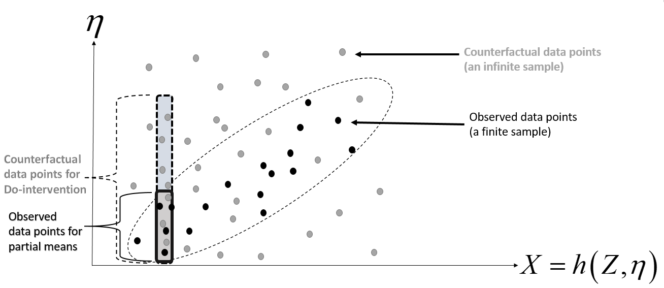
Figure 1: Counterfactual Machinery vs. Partial Means
(Unrestricted vs. Restricted support)

The observed data set is denoted by the black dots and the counterfactual data set is denoted by the gray dots. By construction, the former is randomly drawn from the joint support of $X$ and $\upeta$, while the latter is randomly drawn from the rectangular support $\text{Supp}(X)\times\text{Supp}(\upeta)$. Consequently, the partial means estimate of $\mathbb{E}[Y|\text{do}(X=x)]$ is calculated by using the observed data $X$ and $Y$ in which $X$ and $\upeta$ are jointly dependent as in Figure 1.

Our theoretical result (theorem 7.2) implies that both the kernel as well as the integral equation can be completely characterized by generator functions belonging to $\widetilde{\mathcal{C}}$ and being incorporated in our proposed estimator (in section 8 to follow). To show that, recall the Dirac delta function $\updelta(\cdot)$ and denote,

$$f_{Y,X|Z=z}(y,x)=\int_{0}^{1}\left\{\int_{[0,1]^{d}}\updelta\left(y-\widetilde{g}\left(\widetilde{h}(z,\omega),\omega,\bm{\nu}\right)\right)d\bm{\nu}\right\}\updelta\left(x-\widetilde{h}(z,\omega)\right)d\omega.$$

Next, we propose our estimator and justify the type of Neural network architecture we develop, which involves sequential generator functions. The sequential generator functions estimator is proposed to mimic the underlying data generation process as in a triangular model, where by its very definition, the structural functions are formulated in a sequential manner.

8 Estimation: contaminated GAN (CONGAN)

The formulation of the system of Fredholm equations in (74) (in Appendix A) is used only for achieving the identifiability of $H(y|x)$ and not for estimation. This disparity between identification and estimation is related to the fact that such a system of equations might be ill-posed. Namely, it may provide an estimator which is a discontinuous function of the data and thus, inconsistent (Darolles ., 2011; Newey  Powell, 2003). This issue is resolved here by constructing a novel contaminated GAN (CONGAN) estimator, which is a smooth function of the data. The benefit of the contaminated Neural network is in that it precludes the need to invert the generators in order to account for the posterior distribution of the latent context variable given the observables, which is computationally cumbersome.

Consider a probability space $(\Upomega,\mathcal{F},\mathbb{P})$, a measurable output spaces $(\mathcal{X},\mathcal{Y})$ for the random vector $(X,Y)$, an observed input space $\mathcal{Z}$ for the random variable $Z$ and a latent input space $(\mathcal{U,V})$ for the random vector $(\upomega,\bm{\nu})$. The set of paired measurable functions $\mathcal{G}:(\mathcal{X},\mathcal{U},\mathcal{V})\mapsto\mathcal{Y}$ and $\mathcal{H}:(\mathcal{Z},\mathcal{U})\mapsto\mathcal{X}$ map from an input space (observed and latent space) to the output space. These functions are termed generator functions designated to produce random samples. We consider also $\mathcal{D}$ a set of measure functions $d:(\mathcal{X},\mathcal{Y},\mathcal{Z})\mapsto[0,1]$ referred to as discriminators. Their role is classifying the input space as either real or synthetic. Let $\mu$ be a measure on $(\mathcal{X},\mathcal{Y})$, we make the following assumption (Singh ., 2018):

Assumption 8.1.

$\forall(\widetilde{h},\widetilde{g})\in\mathcal{(G,H)}$ the distributions of $\widetilde{g}(X,\omega,\nu)$ and $\widetilde{h}(Z,\omega)$ are absolutely continuous with respect to $\mu$. The joint distribution of $(Y,X,Z)$ is absolutely continuous with respect to $\mu$.

We define the contaminated GAN (CONGAN) approach as an extension of the original GAN (Goodfellow ., 2014) as follows:

$$V(d,(\widetilde{h},\widetilde{g}))=\left\{\mathbb{E}_{\begin{subarray}{c}X,Y,Z\sim F_{X,Y,Z}\end{subarray}}\left[\log\left(d(X,Y,Z)\right)\right]+\mathbb{E}_{\begin{subarray}{c}\upomega\sim U[0,1]\\ \nu\sim U[0,1]\\ Z\sim F_{Z}\end{subarray}}\left[\log\left(1-d\left(\widetilde{h}(Z,\omega),\widetilde{g}\left(\widetilde{h}(z,\omega),\omega,\bm{\nu}\right)\right),Z\right)\right]\right\}$$ (32)

The key difference between the original GAN and our proposed CONGAN is entirely related to the sequential construction of the generator functions (the generator function $\widetilde{h}$ belongs to the input of the generator function $\widetilde{g}$) both share the noise $\omega$ as appears under the contamination braces in (32). Namely, (32) is reduced to the original GAN when $\widetilde{h}(Z,\omega)$ is substituted with $X$ and the expectation of the CON braces is taken w.r.t $X$, $Z$ and $\bm{\nu}$ rather than w.r.t $\bm{\nu},\omega$ and $Z$.

The optimal discriminator assigns values close to $1$ given data from the joint distribution of $(X,Y,Z)$ and assigns values close to zero given data from the distribution obtained by the generator functions $(\widetilde{h},\widetilde{g})$. Thus, the optimal $d$ given a fixed pair of generator functions $(\widetilde{h},\widetilde{g})$ is:

$$d=\underset{d\in\mathcal{D}}{\arg\max}\hskip 2.5ptV(\cdot,(\widetilde{h},\widetilde{g}))$$ (33)

Then, the optimal pair of generator functions $(\widetilde{h},\widetilde{g})$ is the one solving the $\min\max$ problem:

$$(\widetilde{h},\widetilde{g})=\underset{(\widetilde{h},\widetilde{g})\in\mathcal{(G,H)}}{\arg\min}\hskip 2.5pt\left\{\underset{d\in\mathcal{D}}{\arg\max}\hskip 2.5ptV(d,(\widetilde{h},\widetilde{g}))\right\}$$ (34)

Define $f_{Y,X|Z}^{\text{O}}(y,x|z;\widetilde{g},\widetilde{h}):=\frac{\partial^{2}}{\partial x\partial y}F_{Y,X|Z}^{\text{O}}(y,x|z;\widetilde{g},\widetilde{h})$ and suppose that assumption 8.1 holds. Then following Theorem 2.2 in Singh . (2018),

$$V(d,(\widetilde{h},\widetilde{g}))=\int_{x,y,z}\left\{\log\left(d(x,y,z)\right)f_{Y,X|Z}(y,x|z)+\log\left(1-d(x,y,z)\right)f_{Y,X|Z}^{\text{O}}(y,x|z;\widetilde{g},\widetilde{h})\right\}f_{z}(z)dx\hskip 1.99997ptdy\hskip 1.99997ptdz$$ (35)

$\forall\hskip 1.99997pt(\widetilde{h},\widetilde{g})\in\mathcal{(G,H)}$ and $\forall\hskip 1.99997ptd\in\mathcal{D}$. Hence, for any fixed pair of generators $(\widetilde{h},\widetilde{g})\in\mathcal{(G,H)}$ and $d\in\mathcal{D}$ maximization of $V(d,(\widetilde{h},\widetilde{g}))$ has the form:

$$d(x,y,z)=\frac{f_{Y,X|Z}(y,x|z)}{f_{Y,X|Z}(y,x|z)+f_{Y,X|Z;\widetilde{g},\widetilde{h}}^{\text{O}}(y,x|z)},\hskip 10.00002pt\forall\hskip 1.99997pt(x,y,z)\in\text{Supp}(X,Y,Z)$$ (36)

This yields:

$$\underset{d\in\mathcal{D}}{\max}\hskip 2.5ptV(d,(\widetilde{h},\widetilde{g}))=\int_{x,y,z}\left\{f_{Y,X|Z}(y,x|z)\log\left(\frac{f_{Y,X|Z}(y,x|z)}{f_{Y,X|Z}(y,x|z)+f_{Y,X|Z}^{\text{O}}(y,x|z;\widetilde{g},\widetilde{h})}\right)\right\}f_{z}(z)dx\hskip 1.99997ptdy\hskip 1.99997ptdz$$ (37)

$$+\int_{x,y,z}\left\{f_{Y,X|Z}(y,x|z)\log\left(\frac{f_{Y,X|Z}^{\text{O}}(y,x|z;\widetilde{g},\widetilde{h})}{f_{Y,X|Z}(y,x|z)+f_{Y,X|Z}^{\text{O}}(y,x|z;\widetilde{g},\widetilde{h})}\right)f_{z}(z)dx\hskip 1.99997ptdy\hskip 1.99997ptdz\right\}$$

The result above represents the Nash equilibrium concept, in the sense that both the discriminator as well as the generator players reach their best responses in maximizing their value functions given the other player action (Goodfellow ., 2014). In practice $f_{z}(z)$, $f_{Y,X|Z}(y,x|z)$ and $f_{Y,X|Z}^{\text{O}}(y,x|z;\widetilde{g},\widetilde{h})$ are estimated by a kernel density estimator as a function of some unknown bandwidth $\bm{\upsigma}=(\upsigma_{x},\upsigma_{y},\upsigma_{z})$. This bandwidth is a parameter of the model satisfying the aforementioned Nash equilibrium. Consequently, it obviates the known problematic cross-validation, which requires formidable successive multiple estimations of the likelihood function.

Next we attend to the characterization of our proposed Neural network to be used in the contaminated GANS methodology. For doing so, we denote a feed-forward Neural network consisting of $L$ layers (such that there are $L-1$ hidden layers). In what follows we explain in detail the formulation of the sequential generator functions in this Neural network, presented in the following figure:

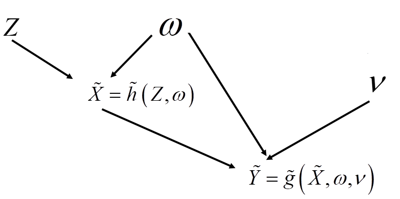
Figure 2: Neural Network with sequential generators ($\widetilde{h}$ and $\widetilde{g}$)

Figure 2 depicts the sequential generation of $\widetilde{X}$ and $\widetilde{Y}$ induced by a triangular model with error-decoupling. By adopting this sequential data generation process, in which $\widetilde{g}$ takes the output of $\widetilde{h}$ as one of its arguments, one can exploit the unrestricted support domain of the latent space in order to construct the observed distribution in (28) as well as the counterfactual distribution in (30). This latent space consists of $\upomega$ and the random disturbance $\nu$. Next, we characterize explicitly the Neural network architecture to estimate these functions.

8.1 Multi-layer neural network with sequential generator functions

Denote the input space of its $\ell$’th layer in the generator functions of $Y$ and $X$ by the column vectors $\bm{\mathcal{Y}}_{\ell-1}$ and $\bm{\mathcal{X}}_{\ell-1}$ of sizes $T_{\ell-1}^{Y}\times 1$ and $T_{\ell-1}^{X}\times 1$, respectively. The parameters associated with these covariate vectors are referred to as weights (slopes) and biases (intercepts) which are denoted by the matrices $\bm{W}_{\ell}^{Y}$ and $\bm{W}_{\ell}^{X}$ of sizes $(T_{\ell}^{Y}+1)\times(T_{\ell-1}^{Y}+1)$ and $(T_{\ell}^{X}+1)\times(T_{\ell-1}^{X}+1)$, respectively. Let $\widetilde{g}$ and $\widetilde{h}$ be the generator functions of $Y$ and $X$, respectively, with parameters $\bm{\upbeta}=(\bm{W}_{1}^{X},...,\bm{W}_{L}^{X})$ and $\bm{\uptheta}=(\bm{W}_{1}^{Y},...,\bm{W}_{L}^{Y})$, defined as:

$$\widetilde{g}(X,\omega,\nu,\bm{\uptheta})=\bm{\mathcal{Y}}_{L},\hskip 10.00002pt\bm{\mathcal{Y}}_{0}=[X,\omega,\nu],\hskip 10.00002pt\bm{\mathcal{Y}}_{\ell}=\upvarphi\left(\bm{W}_{\ell}^{Y}\bm{\mathcal{Y}}_{\ell-1}\right),\hskip 10.00002pt\ell=1,...,L$$ (38)

and

$$\widetilde{h}(Z,\omega;,\bm{\upbeta})=\bm{\mathcal{X}}_{L},\hskip 10.00002pt\bm{\mathcal{X}}_{0}=[Z,\omega],\hskip 10.00002pt\bm{\mathcal{X}}_{\ell}=\upvarphi\left(\bm{W}_{\ell}^{X}\bm{\mathcal{X}}_{\ell-1}\right),\hskip 10.00002pt\ell=1,...,L$$ (39)

where $\upvarphi(\cdot):\mathbb{R}\to C\subset\mathbb{R}$ is some differentiable activation function to be applied element-wise. The input space of the first layer is $(T_{0}^{Y},T_{0}^{X})=(3,2)$ and the output of the last layer is $(T_{L}^{Y},T_{L}^{X})=(1,1)$.

Real and synthetic data are denoted by $\left\{(X_{i},Y_{i},Z_{i})\right\}_{i=1}^{N}$ and $\left\{(\widehat{X}_{i},\widehat{Y}_{i},Z_{i})\right\}_{i=1}^{N}$, respectively, with $\widehat{X}_{i}:=\widetilde{h}(Z_{i},\omega_{0i},\bm{\upbeta})$ and $\widehat{Y}_{i}:=\widetilde{g}(\widehat{X}_{i},\omega_{0i},\nu_{i};\bm{\uptheta})$.

It should be emphasized that by adopting a Shannon-divergence minimization criterion function, we depart from the practice of Wasserstein GAN (WGAN) (Athey ., 2020). Although WGANS can be trained more easily, it requires the utilization of a penalty function to alleviate various optimization difficulties (Gulrajani ., 2017), which may limit the support domain of the generated data distribution (Wei ., 2018). As we deal with counterfactual analysis we aspire to utilize the entire support domain of the data distribution function. Thus, we adopt a Shannon-divergence minimization criterion function, in which the density is evaluated at each point in the data to preserve the original distribution support. We define the following density estimators:

$$\widehat{p}_{\bm{\upsigma}}(x,y,z)=\frac{1}{N}\sum_{i=1}^{N}\frac{1}{\upsigma_{x}}K\left(\frac{X_{i}-x}{\upsigma_{x}}\right)\frac{1}{\upsigma_{y}}K\left(\frac{Y_{i}-y}{\upsigma_{y}}\right)\frac{1}{\upsigma_{z}}K\left(\frac{Z_{i}-z}{\upsigma_{z}}\right)$$ (40)

$$\widehat{q}_{\bm{\upsigma}}(x,y,z)=\frac{1}{N}\sum_{i=1}^{N}\frac{1}{\upsigma_{x}}K\left(\frac{\widehat{X}_{i}-x}{\upsigma_{x}}\right)\frac{1}{\upsigma_{y}}K\left(\frac{\widehat{Y}_{i}-y}{\upsigma_{y}}\right)\frac{1}{\upsigma_{z}}K\left(\frac{Z_{i}-z}{\upsigma_{z}}\right)$$ (41)

Utilizing the smoothing Jensen-Shannon Divergence emanating from (37) (Sinn  Rawat, 2018):

$$\mathcal{K}_{n}(\bm{\uptheta},\bm{\upbeta},\bm{\upsigma})=\frac{1}{N}\sum_{i=1}^{N}\log\frac{\widehat{p}_{\bm{\upsigma}}(X_{i},Y_{i},Z_{i})}{\widehat{p}_{\bm{\upsigma}}(X_{i},Y_{i},Z_{i})+\widehat{q}_{\bm{\upsigma}}(X_{i},Y_{i},Z_{i})}+\frac{1}{N}\sum_{i=1}^{N}\log\frac{\widehat{q}_{\bm{\upsigma}}(\widehat{X}_{i},\widehat{Y}_{i},Z_{i})}{\widehat{p}_{\bm{\upsigma}}(\widehat{X}_{i},\widehat{Y}_{i},Z_{i})+\widehat{q}_{\bm{\upsigma}}(\widehat{X}_{i},\widehat{Y}_{i},Z_{i})}$$ (42)

where $\bm{\upsigma}:=(\upsigma_{x},\upsigma_{y},\upsigma_{z})$ is the bandwidth vector. The optimal generator’s strategy is to minimize the divergence:

$$(\widehat{\bm{\uptheta}}^{(\text{iter+1})},\widehat{\bm{\upbeta}}^{(\text{iter+1})})=\underset{(\bm{\uptheta},\bm{\upbeta})}{\arg\min}\hskip 1.99997pt\mathcal{K}_{n}(\bm{\uptheta},\bm{\upbeta},\bm{\upsigma}^{(\text{iter})})$$ (43)

We attend to the generation of simulated data for the purpose of causal counterfactual inference by using the estimated structural functions. The synthetic data is constructed from the synthetic (estimated) structural functions $\widetilde{g}$ and $\widetilde{h}$, whereas the real data is constructed from the original structural model $g$ and $h$ in (1) and in (2), respectively. The latter will be used as a benchmark for verifying the accuracy of the estimate obtained from the synthetic data.

8.2 Synthetic counterfactual machine vs. partial means estimator (Newey, 1994)

The following equations map an input vector $(Z_{i},\upomega_{i},\widetilde{\upomega}_{i},\nu_{i})$ to an output vector $(X_{\text{real,i}}^{\text{CF}},Y_{\text{real,i}}^{\text{CF}})$ in order to generate the real counterfactual (CF) data set from the structural functions $g$ and $h$:

$$X_{\text{real,i}}^{\text{CF}}=h^{*}\left(Z_{i},\omega_{i}^{\text{real}}\right),\hskip 10.00002pt\omega_{i}^{\text{real}},\widetilde{\omega}_{i}^{\text{real}},\nu_{i}^{\text{real}}\sim U[0,1].$$ (44)

$$Y_{\text{real,i}}^{\text{CF}}=g\left(X_{\text{real,i}},F_{\bm{\epsilon}|\upeta}^{-1}\left(\nu_{i}^{\text{real}}|F_{\upeta}^{-1}\left(\widetilde{\omega}_{i}^{\text{real}}\right)\right)\right).$$ (45)

The following equations map an input vector $(Z_{i},\upomega_{i},\widetilde{\upomega}_{i},\nu_{i})$ to an output vector $(X_{\text{synt,i}}^{\text{CF}},Y_{\text{synt,i}}^{\text{CF}})$ in order to generate the synthetic (synt) counterfactual (CF) data set from the synthetic (estimated) structural functions $\widetilde{g}$ and $\widetilde{h}$:

$$X_{\text{synt,i}}^{\text{CF}}=\widetilde{h}\left(Z,\omega_{i}^{\text{synt}};\bm{\upbeta}\right),\hskip 10.00002pt\omega_{i}^{\text{synt}},\widetilde{\omega}_{i}^{\text{synt}},\nu_{i}^{\text{synt}}\sim U[0,1]$$ (46)

$$Y_{\text{synt,i}}^{\text{CF}}=\widetilde{g}\left(X_{\text{synt,i}},\widetilde{\omega}_{i}^{\text{synt}},\nu_{i}^{\text{synt}};\bm{\uptheta}\right).$$ (47)

Similarly, the following equations map an input vector $(Z_{i},\upomega_{i},\nu_{i})$ to an output vector $(X_{\text{real,i}}^{\text{O}},Y_{\text{real,i}}^{\text{O}})$ in order to generate the real observed (O) data set from the structural functions $g$ and $h$:

$$X_{\text{real,i}}^{\text{O}}=h^{*}\left(Z_{i},\omega_{i}^{\text{real}}\right),\hskip 10.00002pt\omega_{i}^{\text{real}},\nu_{i}^{\text{real}}\sim U[0,1]$$ (48)

$$Y_{\text{real,i}}^{\text{O}}=g\left(X_{\text{real,i}},F_{\bm{\epsilon}|\upeta}^{-1}\left(\nu_{i}^{\text{real}}|F_{\upeta}^{-1}\left(\omega_{i}^{\text{real}}\right)\right)\right),$$ (49)

and the following equations map an input vector $(Z_{i},\upomega_{i},\nu_{i})$ to an output vector $(X_{\text{synt,i}}^{\text{O}},Y_{\text{synt,i}}^{\text{O}})$ in order to generate the synthetic (synt) observed (O) data set from the synthetic (estimated) structural functions $\widetilde{g}$ and $\widetilde{h}$:

$$X_{\text{synt,i}}^{\text{O}}=\widetilde{h}\left(Z,\omega_{i}^{\text{synt}};\bm{\upbeta}\right),\hskip 10.00002pt\omega_{i}^{\text{synt}},\nu_{i}^{\text{synt}}\sim U[0,1]$$ (50)

$$Y_{\text{synt,i}}^{\text{O}}=\widetilde{g}\left(X_{\text{synt,i}},\omega_{i}^{\text{synt}},\nu_{i}^{\text{synt}};\bm{\uptheta}\right).$$ (51)

The estimated conditional expected outcomes given the action in the real data is:

$$\widehat{\mathbb{E}}\left[Y_{\text{real}}|X=x\right]=\widehat{\mathbb{E}}\left[Y_{\text{real}}^{\text{O}}|X_{\text{real}}^{\text{O}}=x\right]=\frac{\frac{1}{N}\frac{1}{\upsigma_{x}}\sum_{i=1}^{N}Y_{\text{real,i}}^{\text{O}}K\left(\frac{X_{\text{real,i}}^{\text{O}}-x}{\upsigma_{x}}\right)}{\frac{1}{N}\frac{1}{\upsigma_{x}}\sum_{i=1}^{N}K\left(\frac{X_{\text{real,i}}^{\text{O}}-x}{\upsigma_{x}}\right)}.$$ (52)

The estimated conditional expected outcomes given the action in the synthetic (synt) data is:

$$\widehat{\mathbb{E}}\left[Y_{\text{synt}}|X=x\right]=\widehat{\mathbb{E}}\left[Y_{\text{synt}}^{\text{O}}|X_{\text{synt}}^{\text{O}}=x\right]\frac{\frac{1}{N}\frac{1}{\upsigma_{x}}\sum_{i=1}^{N}Y_{\text{synt,i}}^{\text{O}}K\left(\frac{X_{\text{synt,i}}^{\text{O}}-x}{\upsigma_{x}}\right)}{\frac{1}{N}\frac{1}{\upsigma_{x}}\sum_{i=1}^{N}K\left(\frac{X_{\text{synt,i}}^{\text{O}}-x}{\upsigma_{x}}\right)}.$$ (53)

The estimated counterfactual expected outcomes given the action in the real data is:

$$\widehat{\mathbb{E}}\left[Y_{\text{real}}|\text{do}(X_{\text{real}}=x)\right]=\widehat{\mathbb{E}}\left[Y_{\text{real}}^{\text{CF}}|X_{\text{real}}^{\text{CF}}=x\right]=\frac{\frac{1}{N}\frac{1}{\upsigma_{x}}\sum_{i=1}^{N}Y_{\text{real,i}}^{\text{CF}}K\left(\frac{X_{\text{real,i}}^{\text{CF}}-x}{\upsigma_{x}}\right)}{\frac{1}{N}\frac{1}{\upsigma_{x}}\sum_{i=1}^{N}K\left(\frac{X_{\text{real,i}}^{\text{CF}}-x}{\upsigma_{x}}\right)}.$$ (54)

The estimated counterfactual expected outcomes given the action in the synthetic (synt) data is:

$$\widehat{\mathbb{E}}\left[Y_{\text{synt}}|\text{do}(X_{\text{synt}}=x)\right]=\widehat{\mathbb{E}}\left[Y_{\text{synt}}^{\text{CF}}|X_{\text{synt}}^{\text{CF}}=x\right]\frac{\frac{1}{N}\frac{1}{\upsigma_{x}}\sum_{i=1}^{N}Y_{\text{synt,i}}^{\text{CF}}K\left(\frac{X_{\text{synt,i}}^{\text{CF}}-x}{\upsigma_{x}}\right)}{\frac{1}{N}\frac{1}{\upsigma_{x}}\sum_{i=1}^{N}K\left(\frac{X_{\text{synt,i}}^{\text{CF}}-x}{\upsigma_{x}}\right)}.$$ (55)

The partial means estimator (Newey, 1994) is presented here as a benchmark, as it is applied to the observed data set, unlike the counterfactual expression applied to the counterfactual dataset in (54):

$$\widehat{\widehat{\mathbb{E}}}\left[Y_{\text{real}}|\text{do}(X_{\text{real}}=x)\right]=\frac{1}{N}\sum_{i=1}^{N}\widehat{\mathbb{E}}\left[Y_{\text{real}}^{\text{O}}|X_{\text{real}}^{\text{O}}=x,\upomega^{\text{real}}=\omega_{i}^{\text{real}}\right]$$ (56)

with

$$\widehat{\mathbb{E}}\left[Y_{\text{real}}^{\text{O}}|X_{\text{real}}^{\text{O}}=x,\upomega^{\text{real}}=\omega\right]=\frac{\frac{1}{N}\frac{1}{\upsigma_{x}}\frac{1}{\upsigma_{\omega}}\sum_{i=1}^{N}Y_{\text{real,i}}^{\text{O}}K\left(\frac{X_{\text{real,i}}^{\text{O}}-x}{\upsigma_{x}}\right)K\left(\frac{\omega_{i}^{\text{real}}-\omega}{\upsigma_{\omega}}\right)}{\frac{1}{N}\frac{1}{\upsigma_{x}}\frac{1}{\upsigma_{\omega}}\sum_{i=1}^{N}K\left(\frac{X_{\text{real,i}}^{\text{O}}-x}{\upsigma_{x}}\right)K\left(\frac{\omega_{i}^{\text{real}}-\omega}{\upsigma_{\omega}}\right)}.$$ (57)

We note that $\widehat{\widehat{\mathbb{E}}}\left[Y_{\text{real}}|\text{do}(X_{\text{real}}=x)\right]$ and $\widehat{\mathbb{E}}\left[Y_{\text{real}}|\text{do}(X_{\text{real}}=x)\right]$ are different empirical objects. In the former $Y_{\text{real}}^{\text{O}}$, available only in theory (as $\upeta$ is unknown), is generated from the same realization of $\upomega$ generated $X_{\text{real}}^{\text{O}}$, while in the latter $Y_{\text{real}}^{\text{CF}}$ is generated by $\widetilde{\upomega}$ (another realization of $\upomega$) which is independent of $X_{\text{real}}^{\text{O}}$. Consequently, $\widehat{\mathbb{E}}\left[Y_{\text{real}}|\text{do}(X_{\text{real}}=x)\right]$ is expected to be more accurate by not being limited to the the joint support of $\upomega$ and $X_{\text{real}}^{\text{O}}$.

Equation (56) utilizes $\upomega:=F_{\upeta}(\upeta)$ which is unobserved in the data. In case of strict monotonicity the following holds $F_{\upeta}(\upeta)=F_{X|Z}(X|Z)$ (Imbens  Newey, 2009). Thus, one can construct $V_{\text{real,i}}:=\widehat{F}_{X|Z}(X_{\text{real,i}}^{\text{O}}|Z_{i})$ to estimate $\upeta$ (up to normalization) and employ the partial means estimator as follows:

$$\widehat{\widehat{\mathbb{E}}}\left[Y_{\text{real}}|\text{do}(X_{\text{real}}=x)\right]=\frac{1}{N}\sum_{i=1}^{N}\widehat{\mathbb{E}}\left[Y_{\text{real}}^{\text{O}}|X_{\text{real}}^{\text{O}}=x,V_{\text{real}}=V_{\text{real,i}}\right]$$ (58)

This is the benchmark used for comparison of our results. The reasons for choosing equation (58) for comparison are: (i) to show that our counterfactual goes beyond conditional quantiles of observables captured by the transformation above (violation of monotonicity) and further (ii) to demonstrate our approach performance in the presence of restricted support which is an acute problem in empirical research regardless of the presence or absence of monotonicity (Chernozhukov ., 2020).

9 Simulations

In what follows we verify our proposed estimator’s performance by employing monte-carlo simulations. The section has two rules: the first is to verify our model performance when the underlying model is characterized by intrinsically non-monotonic structural equations for $X$ and $Y$. The second is to use various examples representing important and widely used economic models of supply and demand which lie in the heart of the economic science, such as: the “backward-bending” supply curve of labor (Hanoch, 1965); the Almost Ideal Demand System (AIDS) (Deaton  Muellbauer, 1980); the Constant Elasticity of Substitution (CES) production function (Sato, 1967) as well as the Translog utility function (Christensen ., 1975), which may also affect the demand and supply curves. A specific model of demand and supply functions have been discussed in Blundell  Matzkin (2014) under the assumption of strict monotonicity in the unobserved non-additively-separable error terms. We however, attend to a more general (and non-monotonic) functional form for various economic phenomena.

The various widely used economic models discussed above are estimated from data sets generated by the following data generation processes:

1. Trans-log utility functions:

   $$h_{1}(Z,\upeta)=\upalpha_{0}+\upalpha_{1}\log(Z)+\upalpha_{2}\log(\upeta)+\upalpha_{3}\log^{2}(Z)+\upalpha_{4}\log^{2}(\upeta)+\upalpha_{5}\log(Z)\log(\upeta)$$ (59)

   $$g_{1}(X,\bm{\epsilon})=\upbeta_{0}+\upbeta_{1}\log(X)+\upbeta_{2}\log(\epsilon)+\upbeta_{3}\log^{2}(X)+\upbeta_{4}\log^{2}(\epsilon)+\upbeta_{5}\log(X)\log(\epsilon)$$ (60)

2. Almost Ideal Demand System (AIDS) functions:

   $$h_{2}(Z,\upeta)=h_{1}(Z,\upeta)+\upalpha_{6}(Z\upeta)^{\uprho}$$ (61)

   $$g_{2}(X,\bm{\epsilon})=g_{1}(X,\bm{\epsilon})+\upbeta_{6}(X\epsilon)^{\uprho}$$ (62)

3. Constant Elasticity of Substitution (CES) production functions:

   $$h_{3}(Z,\upeta)=\upalpha_{1}\left[\upalpha_{2}Z^{-\uprho}+\upalpha_{3}\upeta^{-\uprho}\right]^{-\upalpha_{4}/\uprho}$$ (63)

   $$g_{3}(X,\bm{\epsilon})=\upbeta_{1}\left[\upbeta_{2}X^{-\uprho}+\upbeta_{3}\epsilon^{-\uprho}\right]^{-\upbeta_{4}/\uprho}$$ (64)

4. Backward-bending supply curves for $\upalpha_{1}=0,\upalpha_{2}=1$ and $\upbeta_{1}=0,\upbeta_{2}=1$:

   $$h_{4}(Z,\upeta)=\exp(Z\upeta-\upalpha_{1}Z)-\upalpha_{2}(Z\upeta-\upalpha_{1}Z)$$ (65)

   $$g_{4}(X,\bm{\epsilon})=\exp(X\epsilon-\upbeta_{1}X)-\upbeta_{2}(X\epsilon-\upbeta_{1}X)$$ (66)

5. A generalized cobb-Douglas production function (Cobb-Douglas is obtained for $\upalpha_{1}=\upalpha_{2}=0$ and $\upbeta_{1}=\upbeta_{2}=0$):

   $$h_{5}(Z,\upeta)=\upalpha_{1}Z+\upalpha_{2}\upeta+\upalpha_{3}Z^{\upalpha_{4}}\upeta^{\upalpha_{5}}$$ (67)

   $$g_{5}(X,\bm{\epsilon})=\upalpha_{1}X+\upalpha_{2}\epsilon+\upbeta_{3}X^{\upbeta_{4}}\epsilon^{\upbeta_{5}}$$ (68)

6. Nonlinearly non-additively-separable error terms

   $$h_{6}(Z,\upeta)=\upalpha_{1}\tanh(\upalpha_{2}Z+\upalpha_{3}\upeta)+\upalpha_{4}\tanh(\upalpha_{5}\upeta)$$ (69)

   $$g_{6}(X,\bm{\epsilon})=\upbeta_{1}\tanh(\upbeta_{2}Z+\upbeta_{3}\epsilon)+\upbeta_{4}\tanh(\upbeta_{5}\epsilon)$$ (70)

   with $\tanh(x)=\frac{\exp(x)-\exp(-x)}{\exp(x)+\exp(-x)}$ commonly known as hyperbolic tangent.

The error terms are generated as follows: $\upeta,\nu\sim N(0,1)$ such that $\upeta\mathchoice{\mathrel{\hbox to0.0pt{$\displaystyle\perp$\hss}\mkern 2.0mu{\displaystyle\perp}}}{\mathrel{\hbox to0.0pt{$\textstyle\perp$\hss}\mkern 2.0mu{\textstyle\perp}}}{\mathrel{\hbox to0.0pt{$\scriptstyle\perp$\hss}\mkern 2.0mu{\scriptstyle\perp}}}{\mathrel{\hbox to0.0pt{$\scriptscriptstyle\perp$\hss}\mkern 2.0mu{\scriptscriptstyle\perp}}}\nu$,

$$\epsilon=\upgamma_{1}\upeta\nu+\upgamma_{2}\upeta+\upgamma_{3}\nu,\hskip 10.00002pt\upgamma_{1},\upgamma_{2},\upgamma_{3}\in\left\{-3,-2,-1,0,1,2,3\right\}$$ (71)

We consider various specifications for the structural equations of $X$ and $Y$, each one is chosen from the following functions: the Trans-log utility functions in (i); the Almost Ideal Demand System (AIDS) functions in (ii); the Constant Elasticity of Substitution (CES) production functions in (iii); the backward-bending supply curves in (iv); a Cobb-Douglas production function in (v) and the hyperbolic tangent model in (vi). For sake of generality, for each of these model specifications, we verify our model performance under different Neural network architectures, such that for each given architecture we generated $100$ data sets. These data sets are used to calculate the means and the standard error of our estimates. Such depth of simulations can be carried out only by parallel computing that can handle very demanding computations at a reasonable time in order to explore many specifications and variations of data generation processes.

Each of tables 1-5 (appendix D) summarizes the results obtained from Monte-Carlo simulations generating $100$ data sets, each consisting of $10,000$ observations from specified structural model (data generation process) includes the following columns: a specific quantile of the action variable (column ($a$)); the mean value (over data sets) of the action variable in this quantile (column ($b$)); the mean (over data sets) of the estimated expected counterfactual outcome (given the action variable) using the real and synthetic data in (column ($c$)) and (column $(d)$), respectively; the mean (over data sets) of the estimated expected outcome (given the action variable) using the real data in (column $(e)$) and (column $(f)$), respectively; the control variable results (Imbens  Newey, 2009) represent the counterfactual expected outcome that would be obtained by evaluating the latent context variable through the imposition of strict monotonicity (column $(g)$); and the partial means results (Newey, 1994) represent the counterfactual expected outcome that would be obtained if the context were known (column $(h)$);

We quantify the proximity of the synthetic data set generated by the synthetic generator functions $\widetilde{g}$ and $\widetilde{h}$ to the real data set generated by the “true” generator functions, $g$ and $h$. For tractability, our analysis disentangles the restricted support and divergence from strict monotonicity issues by using the following four criteria:

1. Observed Similarity between $\widehat{\mathbb{E}}\left[Y_{\text{real}}^{\text{O}}|X_{\text{real}}^{\text{O}}=x\right]$ and $\widehat{\mathbb{E}}\left[Y_{\text{synt}}^{\text{O}}|X_{\text{synt}}^{\text{O}}=x\right]$ in (52) and (53), respectively. It measures the resemblance between the estimates of the observed expected outcome of $Y$ (at each quantile of $X$) in the synthetic and real data sets.

2. Counterfactual Similarity between $\widehat{\mathbb{E}}\left[Y_{\text{real}}^{\text{CF}}|X_{\text{real}}^{\text{CF}}=x\right]$ and $\widehat{\mathbb{E}}\left[Y_{\text{synt}}^{\text{CF}}|X_{\text{synt}}^{\text{CF}}=x\right]$ in (54) and (55), respectively. It measures the resemblance between the estimates of the counterfactual expected outcome of $Y$ (at each quantile of $X$) in the synthetic and real data sets.

3. Strict monotonicity by comparing the estimated counterfactual results in (56), which does not rely on monotonicity, to the partial means estimate under monotonicity in (58). Both of these estimators utilize the restricted empirical support only. The degree of non-monotonicity is quantified in these simulations by comparing the results that would have been obtained if $\upomega$ were known (the partial means estimator) to the actual results obtained by using $\widehat{\upomega}=$, an estimate of it (the control variable estimator). Consequently, a negligible disparity between the estimates of the control variable and the partial means indicate that the monotonicity assumption could have been imposed.

4. Restricted support by comparing our real data counterfactual estimate in (54) utilizing the unrestricted support to the partial means in (56) utilizing the restricted support. Both of these estimators do not rely on monotonicity. However, the partial means estimator is available only in theory in which latent context is treated as known. Any disparity between the partial means and the real counterfactual expected outcomes are related to discrepancies between the empirical and theoretical support of the context and action variable.

In the theoretical model we have shown that the importance of allowing for measure-preserving transformations when only distributional similarity is required. That is, we are interested in measuring the similarity between the empirical distributions of two sequences of estimates collected from the Monte Carlo simulations. Each sequence belongs to a different estimator. Thus, in the empirical application we opted for the Sliced-Wasserstein Distance (SWD) (Manole ., 2019), because it is designated for the comparison of two empirical distributions in a non-parametric manner. For robustness, these distributions must be compared over quantiles in the interior of the distribution to avoid the imposition of parametric assumptions regarding the tail behaviour of each distribution. Thus, we specify a scalar $\Lambda\in(0,0.5)$ for which $[\Lambda,1-\Lambda]$ denotes an interval of quantiles in the interior of the distribution. Using the aforementioned (SWD) methodology we append an asterisk and a dagger to indicate sequences of estimates with similar empirical distributions (over the Monte Carlo simulations) to those of the real counterfactual and the real observed results, respectively. Consequently, we perform these similarity tests by comparing distributions using only quantiles in the interval $[0.05,0.95]$ at significance level of $95\%$.

Summary statistics of results are presented in tables 1-5 (appendix D). Entries represent average (standard error) of estimates obtained from $100$ samples of $10,000$ observations each. The overall picture emerging from the simulations, as appears in the tables, points to the superiority of our proposed casual inference. This is apparent from the similarity (in the SWD sense) between the real (column $(e)$) and synthetic (column ($f$)) counterfactual results, which appears in the various tables representing different known economics models. In particular, when juxtaposed on the much different and inferior results of existing models as shown in columns ($g$) and ($h$). Basically, existing causality models hardly successfully reconstruct the real counterfactual results. Further, even when choosing a monotonic structural form like the CES in table 1 (appendix D), results when applying conventional casual inference (column ($g$) and ($h$)) are still inaccurate due to an improper restricted support domain. As can be be seen, our model produces real and synthetic counterfactual results (in bold) which obey SWD similarity. For instance, in the 80th quantile of $X$, we report an estimate of (standard error) (table 1, column ($e$)) 13.94 (0.344) for the real counterfactual and (table 1, column ($f$)) 14.13 (0.553) for the synthetic counterfactual. The indication that the empirical support domain is restricted is based on the fact that the real counterfactual estimates are SWD different from the partial means estimates (as described in criterion (iv)). Just as an example, in the 90th quantile of $X$, we report an estimate of (table 1, column ($e$)) 15.73 (0.728) for the real counterfactual and (table 1, column $(h)$) 20.43 (0.960) for the partial means. The high similarity between the average estimates of the control variable (column $(g)$) and the partial means (column $(h)$) indicates that indeed there is no statistical evidence for the violation of strict monotonicity (as described in criterion 6). For instance, in the 5th quantile of $X$, we get the estimates (standard error) of (table 1, column $(g)$) 6.98 (0.338) for the control variable and (table 1, column $(h)$) 6.96 (0.276) for the partial means; in the 25th quantile of $X$, the estimate is (table 1, column $(g)$) 8.52 (0.213) for the control variable and (table 1, column $(h)$) 8.51 (0.188) for the partial means; in the 75th quantile of $X$, it is (table 1, column $(g)$) 15.58 (0.338) for the control variable and (table 1, column $(h)$) 15.59 (0.276) for the partial means.

In table 2 (appendix D) we apply the simulations to the known Translog function which is non-monotonic. The synthetic counterfactual results are not statistically different than the real counterfactual results. For instance, in the 25th quantile of $X$, we report an estimate of (table 2, column ($e$)) 16.63 (0.175) for the real counterfactual and (table 2, column ($f$)) 16.61 (0.407) for the synthetic counterfactual. However, the common practice results are extremely inaccurate in magnitudes (columns $(g)$ and $(h)$). In fact, the non-monotonicity is expressed by the disparity between the control function and the partial means estimates. Just as an example, in the 20th quantile of $X$, the estimate is (table 2, column $(g)$) 20.95 (1.087) for the control variable and (table 2, column $(h)$) 14.71 (0.857) for the partial means. In this specific quantile there is also a disparity between the empirical and restricted supports, captured by the gap between real counterfactual and the partial means estimates. For instance, in the 15th quantile of $X$, it is (table 2, column ($e$)) 15.88 (0.190) for the real counterfactual and (table 2, column $(h)$) 13.53 (0.959) for the partial means.

The entries in table 3 (appendix D) the estimates of the hyperbolic tangent form where the strict monotonicity is violated. Applying the our offered model produces very accurate results and exhibits insignificant statistical difference between the real and synthetic interventional distributions (columns $(e)$ and $(f)$). However, the common practice results are extremely inaccurate in both magnitudes and signs (columns $(g)$ and $(h)$). The violation of monotonicity is expressed by a strong disparity between the control function and the partial means estimates. For instance, the 20th quantile of $X$, we report an estimate of (table 3, column $(g)$) -0.18 (0.291) for the control variable and (table 3, column $(h)$) -0.56 (0.189) for the partial means. There is also a disparity between the empirical and restricted supports, captured by the gap between real counterfactual and the partial means estimates. E.g., in the 15th quantile of $X$, we report an estimate of (table 3, column ($e$)) -0.17 (0.038) for the real counterfactual and (table 3, column $(h)$) -0.70 (0.212) for the partial means.

The entries in table 4 (appendix D) exhibit estimates of the well-known demand function (AIDS). This very well-known functional form is intrinsically non-monotonic. Applying the our offered model produces very accurate results and exhibits insignificant statistical difference between the real and synthetic interventional distributions (columns $(e)$ and $(f)$). For instance, in the 65th quantile of $X$, we report an estimate of (table 4, column ($e$)) 16.71 (0.188) for the real counterfactual and (table 4, column ($f$)) 16.65 (0.348) for the synthetic counterfactual. However, as can be seen results largely demonstrate the failure to mimic the real counterfactual distribution when applying conventional casual inference (column ($g$) and ($h$)). For instance, in the 90th quantile of $X$, we report an estimate of (table 4, column ($e$)) 22.79 (0.669) for the real counterfactual and (table 4, column $(h)$) 26.58 (0.975) for the partial means; For this quantile, the synthetic counterfactual result (table 4, column ($f$)) is 21.66 (0.758). For instance, in the 55th quantile of $X$, we report an estimate of (table 4, column $(g)$) 21.16 (1.101) for the control variable and (table 4, column $(h)$) 16.67 (0.748) for the partial means; For this quantile, the real counterfactual result is (table 4, column ($e$)) 16.06 (0.195) and the synthetic counterfactual result is (table 4, column ($f$)) 16.09 (0.344). There is also a disparity between the empirical and restricted supports, captured by the gap between real counterfactual and the partial means estimates.

The entries in table 5 (appendix D) represent those emerging from the estimation of backward-bending supply curve. In this instance, monotonicity is intrinsically violated. This is attested to the disparity between the control function and the partial means estimates in both magnitude as well as in sign, which in reality may lead to wrong public policy. For instance, in the 35th quantile of $X$, we report an estimate of (table 5, column $(g)$) -0.33 (0.135) for the control variable and (table 5, column $(h)$) 0.33 (0.091) for the partial means. Applying our offered model produces very accurate results and exhibits insignificant statistical difference between the real and synthetic interventional distributions (columns $(e)$ and $(f)$). Just as an example, in the 60th quantile of $X$, the real counterfactual result (table 5, column $(e)$) is 0.61 (0.040) and the synthetic counterfactual result (table 5, column $(f)$) is 0.59 (0.093). Further, below the 40’th quantile it can be seen that there is a disparity between the empirical and restricted supports, captured by the gap between real counterfactual and the partial means estimates. In another instance, in the 25th quantile of $X$, we report an estimate of (table 5, column ($e$)) 0.47 (0.033) for the real counterfactual and (table 5, column $(h)$) 0.21 (0.087) for the partial means. The synthetic counterfactual result is (table 5, column ($f$)) 0.44 (0.109) indicating that it is not statistically different than the real result.

To sum up, the observed and counterfactual similarity criteria (i) and (ii) tables 1-5 (appendix D) developed in this paper demonstrate the high accuracy of the synthetic counterfactual machinery relative to the real data counterfactual result. In terms of sensitivity to the violation of the strict monotonicity assumption, as captured by criterion 6, our proposed estimator produces accurate results regardless of the absence or presence of monotonicity and outperforms control variable existing approach. In terms of sensitivity to the violation of unrestricted support domain, as captured by criterion (iv), our proposed estimator outperforms both the partial means as well as the control variable estimators, by mimicking the results obtained for the real data counterfactual outcome. It emphasized the results generated by the aforementioned existing models produce results that are inaccurate both in magnitude and sign of the estimates.

10 Conclusion

Different latent contexts may affect the relations between cause and outcome and hence can have significant ramification for causal relations and inference. We develop a novel identification strategy as well as a new estimator for triangular models in the presence of non-separable disturbances, which unlike the common practice, does not rely on the strict monotonicity assumption. The key result of this identifiability approach is the explicit characterization of the distributional relationship between the latent context variable and the vector of observables through Fredholm integral equations governed by generator functions and an unknown kernel function, inducing a non-monotonic inverse problem. The role of these generator functions is two-fold: (i) to characterize the unknown kernel function induced by these generator functions and (ii) to ensure that the estimator of the unknown quantity is a continuous function of the data given this unknown kernel function. This very formulation facilitates the establishment of uniqueness of the interventional distribution given the observables. Furthermore, we develop a novel CONGAN estimator based on a feed-forward Neural network architecture generating a synthetic counterfactual distribution. This synthetic distribution represents various combinations of actions, outcomes and contexts, rarely available in finite samples. In the simulations, the proposed estimator’s performance in finite samples has been validated in several aspects by testing various data generation processes each associated with the commonly employed structural functions: Cobb-Douglas, AIDS, CES, Translog and backward-bending supply models. It can be seen that our model generates synthetic data mimicking the behavior in the real data (in terms of SWD similarity). This comparison has been done for different quantiles of the action variable. Our results are also compared to both the monotonic control variable as well as partial means estimators. In some of these models, the counterfactual results obtained by the conventionally used partial means estimator, largely deviate from the benchmark real data results in quantity and sign. This may in reality have important ramifications as to the proper public policy.

In future work, our framework can be incorporated in dynamic models as well as panel models to capture the dependence of the action and outcome on past events through a different Neural network architecture, such as recurrent Neural networks.

Appendices

Appendix A An integral equation for the intervention

In this section we derive an integral equation relating the unknown intervention $H(y|x)$ to known quantities. Recall that Eq. (7) for $H(y|x)$ is fully characterized by the quantities $f_{\upeta}(\cdot)$ and $F_{Y|X=x,\upeta=\eta}(y)$. Unfortunately, both of these quantities are unknown, since $\upeta$ is unobserved.

For future use, from this point on, instead of working with the disturbance $\eta$, we make a change of variables and work with its normalized random variable

$$\upomega=F_{\upeta}(\upeta),$$ (72)

which is distributed as $U[0,1]$.

Towards our goal of proving that $H(y|x)$ is identifiable, we next formulate the relationship between the unknown quantity $F_{Y|X,\upomega}$ and the (known) distribution $F_{Y|X,Z}$ through an integral equation. This relation is stated in the following lemma is proven in Appendix E.

Lemma .1.

Let $(X,Y,Z,\upeta,\bm{\epsilon})$ be distributed according to the triangular model in (1) and (2). Under assumptions 3.1 and 3.2.a the following integral equation holds $\forall(x,y,z)\in\text{Supp}(X,Y,Z)$,

$$F_{Y|X=x,Z=z}(y)=\text{Pr}(Y\leq y|X=x,Z=z)=\int_{0}^{1}F_{Y|X=x,\upomega=\omega}(y)f_{\upomega|X=x,Z=z}(\omega)d\omega.$$ (73)

The entire variation in the estimable quantity $F_{Y|X=x,Z=z}(y)$ in the LHS of the system in (73) is propagated by $Z$. Such variation provides an indirect information regarding $\upeta$ through the integral equations (73). For sake of brevity, we rewrite Eq. (73) as follows,

$$G_{x,y}(z)=\int_{0}^{1}\upgamma_{x,y}(\omega)k_{x}(z,\omega)d\omega\quad\forall(x,y)\in\text{Supp}(X,Y).$$ (74)

where $G_{x,y}(z):=F_{Y|X=x,Z=z}(y)$ is the observed quantity, $k_{x}(z,\omega):=f_{\upomega|X=x,Z=z}(\omega)$ is an unknown kernel function and

$$\upgamma_{x,y}(\omega):=F_{Y|X=x,\upomega=\omega}(y)$$ (75)

is another unknown function. In terms of these quantities, Eq. (7) can be written as

$$H(y|x)=\int_{0}^{1}\upgamma_{x,y}(\omega)d\omega,$$ (76)

Note that Eq. (74) is an inhomogeneous Fredholm integral equation of the first kind. In this equation, the left hand side is known, whereas on the right hand side both the kernel as well as the function $\upgamma_{x,y}$ are unknown. In addition, the system of integral equations may be singular due to an unbounded kernel in that for any $(x,z)$ the kernel may be a weighted sum of Dirac delta functions $\updelta(\cdot)$, aggravating the identifiability challenge. Our identifiability strategy for the interventional distribution bypasses these issues. This is done by characterizing an equivalence class of triangular models sharing the same interventional distribution, despite having different kernels, and is treated in the section to follow.

Appendix B Fourier Expansion

Our main building block in achieving identifiability relies on representing the intervention in terms of Fourier series. For doing so, in the following lemma we rely on Carleson’s theorem (Carleson, 1966) for establishing the point-wise (Lebesgue) almost everywhere convergence of Fourier series of $L_{2}$ functions (see proof in appendix E).

Lemma .2.

Suppose that $f_{Y,X|Z=z}$ and $f_{Y,X|Z=z}^{\text{CF}}$ satisfy squares integrability. Namely,

$$\int\int f_{Y,X|Z=z}^{2}(y,x)dydx<\infty\quad\forall z\quad\text{and}\quad\int\int\left[f_{Y,X|Z=z}^{\text{CF}}(y,x)\right]^{2}dydx<\infty\quad\forall z.$$

Thus, $H(y|x)$ can be characterized $\forall(x,y)\in\text{Supp}(X,Y)$ independently of $Z$ as follows,

$$H(y|x)=\left\{f_{X|Z=z}(x)\right\}^{-1}\int_{y^{\prime}}^{y}\left\{\int_{\xi_{1}}\int_{\xi_{2}}\mathbb{E}_{\begin{subarray}{c}Y\sim H(\cdot|X)\\ X\sim F_{X|Z=z}\end{subarray}}\left[\Psi_{\xi_{1}}(-Y)\Psi_{\xi_{2}}(-X)\right]\Psi_{\xi_{2}}(y^{\prime})\Psi_{\xi_{3}}(x)d\xi_{2}d\xi_{3}\right\}dy^{\prime},$$ (77)

and it holds that $\forall z\in\text{Supp}(Z|X=x)$,

$$\mathbb{E}_{\begin{subarray}{c}Y\sim H(\cdot|X)\\ X\sim F_{X|Z=z}\end{subarray}}\left[\Psi_{\xi_{2}}\left(-Y\right)\Psi_{\xi_{3}}\left(-X\right)\right]=\mathbb{E}_{\upomega,\upomega^{\prime},\bm{\nu}}\left[\Psi_{\xi_{3}}\left(-g^{*}\left(h^{*}(z,\upomega),\upomega^{\prime},\bm{\upnu}\right)\right)\Psi_{\xi_{3}}\left(-h^{*}(z,\upomega)\right)\right].$$ (78)

Appendix C Algorithms

We present our algorithms to estimate the counterfactual distribution: Initial parameter settings and Contaminated Generative Adversarial Network (CONGAN).

Algorithm 1 is employed to provide initial estimates for $\bm{\upbeta}$ and $\bm{\uptheta}$ in order to estimate $\widetilde{h}$ and $\widetilde{g}$, respectively. This is achieved by minimizing the negative entropy:

$$\mathcal{L}(\bm{\upbeta},\bm{\uptheta},\bm{\upsigma})=-N^{-1}\sum_{i=1}^{N}\log\frac{1}{\upsigma_{y}}\frac{1}{\upsigma_{x}}J^{-1}\sum_{j=1}^{J}K\left(\frac{\widetilde{g}\left(\widetilde{h}\left(Z_{i},\omega_{j}\right),\omega_{j},\bm{\nu}_{j}\right)-Y_{i}^{\text{O}}}{\upsigma_{y}}\right)K\left(\frac{\widetilde{h}\left(Z_{i},\omega_{j}\right)-X_{i}^{\text{O}}}{\upsigma_{x}}\right),$$

the empirical variant of the following negative entropy: $\mathcal{L}^{*}(\bm{\upbeta},\bm{\uptheta})=-\int\log f_{Y,X|Z}^{\text{O}}(y,x|z;\widetilde{h},\widetilde{g})f_{Z}(z)dydxdz$, with $f_{Y,X|Z}^{\text{O}}(y,x|z;\widetilde{h},\widetilde{g})=\frac{\partial^{2}}{\partial y\partial x}F_{Y,X|Z}^{\text{O}}(y,x|z;\widetilde{h},\widetilde{g})$ in which the right hand side is the cross-partial derivative of the conditional distribution characterized in (28) with respect to $x$ and $y$.

Algorithm 2 of the CONGAN model in (42) is employed to yield the final estimates for $\bm{\upbeta}$ and $\bm{\uptheta}$ as well as the nuisance parameter $\bm{\upsigma}=(\upsigma_{x},\upsigma_{y},\upsigma_{z})$. This is achieved by minimizing:

$$\mathcal{K}_{n}(\bm{\uptheta},\bm{\upbeta},\bm{\upsigma})=\frac{1}{N}\sum_{i=1}^{N}\log\frac{\widehat{p}_{\bm{\upsigma}}(X_{i},Y_{i},Z_{i})}{\widehat{p}_{\bm{\upsigma}}(X_{i},Y_{i},Z_{i})+\widehat{q}_{\bm{\upsigma}}(X_{i},Y_{i},Z_{i})}+\frac{1}{N}\sum_{i=1}^{N}\log\frac{\widehat{q}_{\bm{\upsigma}}(\widehat{X}_{i},\widehat{Y}_{i},Z_{i})}{\widehat{p}_{\bm{\upsigma}}(\widehat{X}_{i},\widehat{Y}_{i},Z_{i})+\widehat{q}_{\bm{\upsigma}}(\widehat{X}_{i},\widehat{Y}_{i},Z_{i})}.$$ (.1)

Input : A sequence $\left\{(X_{i},Y_{i},Z_{i})\right\}_{i=1}^{N}$ of independent realizations from $F_{X,Y,Z}$.

Output : A pair of sequential generator functions $\left\{\widetilde{h}(\cdot,\cdot;\bm{\upbeta}),\widetilde{g}(\cdot,\cdot,\cdot;\bm{\uptheta})\right\}$.

1 initialization of $\bm{\upbeta}$ and $\bm{\uptheta},\upsigma_{x},\upsigma_{y}$;

2 $\text{tol}=10^{-16}$;

3 $\text{gap}=0$;

4 $\text{iter}=0$;

5 $\Lambda=0.01$;

6 $\text{Max.Iterations}=10,000$;

7 while $\text{gap}\geq\text{tol}$ and $\text{iter}\leq\text{Max.Iterations}$ do

8       for $i=1:N$ do

9             for $j=1:J$ do

10                   $\omega[i,j]=U_{1},\hskip 10.00002ptU_{1}\sim U[0,1]$;

11                   $\bm{\nu}[i,j]=U_{2},\hskip 10.00002ptU_{2}\sim U[0,1]$;

12                   $\widehat{X}_{i,j}=\widetilde{h}(Z_{i},\omega[i,j];\bm{\upbeta}^{\text{iter}})$;

13                   $\widehat{Y}_{i,j}=\widetilde{g}(\widehat{X}_{i,j},\omega[i,j],\bm{\nu}[i,j];\bm{\uptheta}^{\text{iter}})$;

14                  

15             end for

16            $\text{density}_{i}=\frac{1}{J}\sum_{j=1}^{J}\frac{1}{\upsigma_{x}}K\left(\frac{\widehat{X}_{i,j}-X_{i}}{\upsigma_{x}}\right)\frac{1}{\upsigma_{y}}K\left(\frac{\widehat{Y}_{i,j}-Y_{i}}{\upsigma_{y}}\right)$;

17            

18            $d_{i,j}=\max\left(\mathds{1}\left\{\widehat{X}_{i,j}\neq X_{i}\right\},\mathds{1}\left\{\widehat{Y}_{i,j}\neq Y_{i}\right\}\right)$;

19             $\widehat{p}_{\bm{\upsigma},i}(X_{i},Y_{i})=\left\{\sum_{j=1}^{J}d_{i,j}\right\}^{-1}\sum_{j=1}^{J}d_{i,j}\frac{1}{\upsigma_{x}}K\left(\frac{\widehat{X}_{i,j}-X_{i}}{\upsigma_{x}}\right)\frac{1}{\upsigma_{y}}K\left(\frac{\widehat{Y}_{i,j}-Y_{i}}{\upsigma_{y}}\right)$;

20            

21       end for

22      

23      $\mathcal{L}^{\text{iter}}=-\frac{1}{N}\sum_{i=1}^{N}\log\left(\max(\text{density}_{i},10^{-14})\right)$;

24       Employing leave-one out entropy estimator (Hall  Morton, 1993);

25       $\mathcal{L}_{\bm{\upsigma}}^{\text{iter}}=-\frac{1}{N}\sum_{i=1}^{N}\log\left(\max(\widehat{p}_{\bm{\upsigma},i}(X_{i},Y_{i}),10^{-14})\right)$;

26       $\left[\begin{matrix}\bm{\upbeta}^{\text{iter}+1}\\ \bm{\uptheta}^{\text{iter}+1}\\ \bm{\upsigma}^{\text{iter}+1}\end{matrix}\right]=\left[\begin{matrix}\bm{\upbeta}^{\text{iter}}\\ \bm{\uptheta}^{\text{iter}}\\ \bm{\upsigma}^{\text{iter}}\end{matrix}\right]-\Lambda\left[\begin{matrix}\nabla_{\bm{\upbeta}}\mathcal{L}^{\text{iter}}\\ \nabla_{\bm{\uptheta}}\mathcal{L}^{\text{iter}}\\ \nabla_{\bm{\upsigma}}\mathcal{L}_{\bm{\upsigma}}^{\text{iter}}\end{matrix}\right]$;

27       $(\upsigma_{x},\upsigma_{y})=\bm{\upsigma}^{\text{iter}+1}$;

28       if $\text{iter}>0$ then

29             $\text{gap}=\mathcal{L}^{\text{iter}}-\mathcal{L}^{\text{iter-1}}$ ;

30            

31       end if

32      $\text{iter}=\text{iter}+1$

33 end while

Algorithm 1 Initial parameter settings

Input : A sequence $\left\{(X_{i},Y_{i},Z_{i})\right\}_{i=1}^{N}$ of independent realizations from $F_{X,Y,Z}$.

Output : A pair of sequential generator functions $\left\{\widetilde{h}(\cdot,\cdot;\bm{\upbeta}),\widetilde{g}(\cdot,\cdot,\cdot;\bm{\uptheta})\right\}$.

1 initialization of $\bm{\upbeta}$ and $\bm{\uptheta},\upsigma_{x},\upsigma_{y},\upsigma_{z}$;

2 $\text{tol}=10^{-16}$;

3 $\text{gap}=0$;

4 $\text{iter}=0$;

5 $\Lambda=0.01$;

6 $\text{Max.Iterations}=10,000$;

7 while $\text{gap}\geq\text{tol}$ and $\text{iter}\leq\text{Max.Iterations}$ do

8       for $i=1:N$ do

9             $\omega[i]=U_{1},\hskip 10.00002ptU_{1}\sim U[0,1]$;

10             $\bm{\nu}[i]=U_{2},\hskip 10.00002ptU_{2}\sim U[0,1]$;

11             $\widehat{X}_{i}=\widetilde{h}(Z_{i},\omega[i];\bm{\upbeta}^{\text{iter}})$;

12             $\widehat{Y}_{i}=\widetilde{g}(\widehat{X}_{i},\omega[i],\bm{\nu}[i];\bm{\uptheta}^{\text{iter}})$;

13            

14       end for

15      for $i=1:N$ do

16             $\widehat{p}_{\bm{\upsigma}}(X_{i},Y_{i},Z_{i})=\max\left(\frac{1}{N}\sum_{j=1}^{N}\frac{1}{\upsigma_{x}}K\left(\frac{X_{j}-X_{i}}{\upsigma_{x}}\right)\frac{1}{\upsigma_{y}}K\left(\frac{Y_{j}-Y_{i}}{\upsigma_{y}}\right)\frac{1}{\upsigma_{z}}K\left(\frac{Z_{j}-Z_{i}}{\upsigma_{z}}\right),10^{-14}\right)$;

17             $\widehat{p}_{\bm{\upsigma}}(\widehat{X}_{i},\widehat{Y}_{i},\widehat{Z}_{i})=\max\left(\frac{1}{N}\sum_{j=1}^{N}\frac{1}{\upsigma_{x}}K\left(\frac{X_{j}-\widehat{X}_{i}}{\upsigma_{x}}\right)\frac{1}{\upsigma_{y}}K\left(\frac{Y_{j}-\widehat{Y}_{i}}{\upsigma_{y}}\right)\frac{1}{\upsigma_{z}}K\left(\frac{Z_{j}-Z_{i}}{\upsigma_{z}}\right),10^{-14}\right)$;

18             $\widehat{q}_{\bm{\upsigma}}(X_{i},Y_{i},Z_{i})=\max\left(\frac{1}{N}\sum_{j=1}^{N}\frac{1}{\upsigma_{x}}K\left(\frac{\widehat{X}_{j}-X_{i}}{\upsigma_{x}}\right)\frac{1}{\upsigma_{y}}K\left(\frac{\widehat{Y}_{j}-Y_{i}}{\upsigma_{y}}\right)\frac{1}{\upsigma_{z}}K\left(\frac{Z_{j}-Z_{i}}{\upsigma_{z}}\right),10^{-14}\right)$;

19             $\widehat{q}_{\bm{\upsigma}}(\widehat{X}_{i},\widehat{Y}_{i},\widehat{Z}_{i})=\max\left(\frac{1}{N}\sum_{j=1}^{N}\frac{1}{\upsigma_{x}}K\left(\frac{\widehat{X}_{j}-\widehat{X}_{i}}{\upsigma_{x}}\right)\frac{1}{\upsigma_{y}}K\left(\frac{\widehat{Y}_{j}-\widehat{Y}_{i}}{\upsigma_{y}}\right)\frac{1}{\upsigma_{z}}K\left(\frac{Z_{j}-Z_{i}}{\upsigma_{z}}\right),10^{-14}\right)$;

20             $\widehat{p}_{i,\bm{\upsigma}}(X_{i},Y_{i},Z_{i})=\max\left(\frac{1}{N-1}\sum_{j\neq i}\frac{1}{\upsigma_{x}}K\left(\frac{X_{j}-X_{i}}{\upsigma_{x}}\right)\frac{1}{\upsigma_{y}}K\left(\frac{Y_{j}-Y_{i}}{\upsigma_{y}}\right)\frac{1}{\upsigma_{z}}K\left(\frac{Z_{j}-Z_{i}}{\upsigma_{z}}\right),10^{-14}\right)$;

21             $\widehat{q}_{i,\bm{\upsigma}}(\widehat{X}_{i},\widehat{Y}_{i},\widehat{Z}_{i})=\max\left(\frac{1}{N-1}\sum_{j\neq i}\frac{1}{\upsigma_{x}}K\left(\frac{\widehat{X}_{j}-\widehat{X}_{i}}{\upsigma_{x}}\right)\frac{1}{\upsigma_{y}}K\left(\frac{\widehat{Y}_{j}-\widehat{Y}_{i}}{\upsigma_{y}}\right)\frac{1}{\upsigma_{z}}K\left(\frac{Z_{j}-Z_{i}}{\upsigma_{z}}\right),10^{-14}\right)$;

22            

23       end for

24      

25      $\mathcal{L}^{\text{iter}}=\frac{1}{N}\sum_{i=1}^{N}\log\frac{\widehat{p}_{\bm{\upsigma}}(X_{i},Y_{i},Z_{i})}{\widehat{p}_{\bm{\upsigma}}(X_{i},Y_{i},Z_{i})+\widehat{q}_{\bm{\upsigma}}(X_{i},Y_{i},Z_{i})}+\frac{1}{N}\sum_{i=1}^{N}\log\frac{\widehat{q}_{\bm{\upsigma}}(\widehat{X}_{i},\widehat{Y}_{i},Z_{i})}{\widehat{p}_{\bm{\upsigma}}(\widehat{X}_{i},\widehat{Y}_{i},Z_{i})+\widehat{q}_{\bm{\upsigma}}(\widehat{X}_{i},\widehat{Y}_{i},Z_{i})}$;

26       Employing leave-one out entropy estimator (Hall  Morton, 1993);

27       $\mathcal{L}_{\bm{\upsigma}}^{\text{iter}}=-\frac{1}{N}\sum_{i=1}^{N}\log(\widehat{p}_{\bm{\upsigma},i}(X_{i},Y_{i},Z_{i}))-\frac{1}{N}\sum_{i=1}^{N}\log(\widehat{q}_{i,\bm{\upsigma}}(\widehat{X}_{i},\widehat{Y}_{i},\widehat{Z}_{i}))$;

28       $\left[\begin{matrix}\bm{\upbeta}^{\text{iter}+1}\\ \bm{\uptheta}^{\text{iter}+1}\\ \bm{\upsigma}^{\text{iter}+1}\end{matrix}\right]=\left[\begin{matrix}\bm{\upbeta}^{\text{iter}}\\ \bm{\uptheta}^{\text{iter}}\\ \bm{\upsigma}^{\text{iter}}\end{matrix}\right]-\Lambda\left[\begin{matrix}\nabla_{\bm{\upbeta}}\mathcal{L}^{\text{iter}}\\ \nabla_{\bm{\uptheta}}\mathcal{L}^{\text{iter}}\\ \nabla_{\bm{\upsigma}}\mathcal{L}_{\bm{\upsigma}}^{\text{iter}}\end{matrix}\right]$;

29       $(\upsigma_{x},\upsigma_{y},\upsigma_{z})=\bm{\upsigma}^{\text{iter}+1}$;

30       if $\text{iter}>0$ then

31             $\text{gap}=\mathcal{L}^{\text{iter}}-\mathcal{L}^{\text{iter-1}}$ ;

32            

33       end if

34      $\text{iter}=\text{iter}+1$

35 end while

Algorithm 2 Contaminated Generative Adversarial Network (CONGAN)

Appendix D Tables

Table 1: Do-intervention (CES supply function (Sato, 1967))
Entries represent average (standard error) of estimates
obtained from $100$ samples of 10,000 observations each
$X=h_{3}\left(\zeta(Z),\zeta(\eta)\right)^{1}$;     $Y=g_{5}(X,\bm{\epsilon})^{2}$;     $\upzeta(x)=1.5+1.5\tanh(0.15x)$
$[\upalpha_{1},\upalpha_{2},\upalpha_{3},\uprho]=[6,0.5,0.5,0.5]$
$[\upbeta_{1},\upbeta_{2},\upbeta_{3}]=[2,1,-0.25]$,    $[\upgamma_{1},\upgamma_{2},\upgamma_{3}]=[1,1,1]$

0.75 $\overset{(a)}{\text{Quantile}}$ of X $\overset{(b)}{X}$ $\mathbb{E}\left[Y|X=x\right]$ $\mathbb{E}\left[Y|\text{do}(X=x)\right]$ $\overset{(c)}{\text{real}}$ $\overset{(d)}{\text{synt}}$ $\overset{(e)}{\text{real}}$ $\overset{(f)}{\text{synt}}$ $\overset{(g)}{\text{IN}}$ $\overset{(h)}{\text{PM}}$ 5 2.79 10.45 10.57^† 9.55 10.06* 6.98 6.96 (0.066) (0.042) (0.092) (0.080) (0.143) (0.338) (0.276) 10 3.29 10.67 10.80^† 9.81 10.30* 7.60 7.59 (0.060) (0.046) (0.081) (0.086) (0.128) (0.288) (0.234) 15 3.56 10.81 10.93^† 9.95 10.43* 7.98 7.97 (0.062) (0.048) (0.074) (0.086) (0.113) (0.245) (0.212) 20 3.77 10.91 11.02^† 10.07 10.54* 8.27 8.25 (0.056) (0.045) (0.073) (0.084) (0.105) (0.231) (0.198) 25 3.94 11.00 11.11^† 10.16 10.62* 8.52 8.51 (0.053) (0.046) (0.075) (0.086) (0.101) (0.213) (0.188) 30 4.11 11.10 11.20^† 10.26 10.71* 8.79 8.77* (0.064) (0.051) (0.080) (0.096) (0.100) (0.201) (0.189) 35 4.37 11.24 11.33^† 10.42 10.86* 9.19 9.17* (0.097) (0.076) (0.100) (0.115) (0.109) (0.194) (0.228) 40 4.87 11.55 11.62^† 10.74 11.16* 10.00 9.98* (0.177) (0.125) (0.160) (0.169) (0.145) (0.273) (0.329) 45 5.24 11.79 11.85^† 10.99 11.39* 10.60 10.58* (0.144) (0.111) (0.179) (0.138) (0.151) (0.270) (0.260) 50 5.53 12.00 12.04^† 11.20 11.58* 11.12 11.08* (0.189) (0.150) (0.221) (0.190) (0.184) (0.350) (0.320) 55 6.04 12.39 12.39^† 11.58 11.93* 12.01 11.96 (0.137) (0.125) (0.226) (0.174) (0.194) (0.271) (0.253) 60 6.44 12.71 12.68^† 11.89 12.22* 12.72 12.68 (0.125) (0.127) (0.257) (0.166) (0.218) (0.247) (0.257) 65 6.86 13.07 13.00^† 12.23 12.54* 13.48 13.45 (0.127) (0.135) (0.315) (0.181) (0.264) (0.282) (0.277) 70 7.37 13.56 13.43^† 12.69 12.97* 14.43 14.41 (0.158) (0.176) (0.403) (0.227) (0.335) (0.346) (0.334) 75 7.98 14.20 13.96^† 13.25 13.49* 15.58 15.59 (0.153) (0.198) (0.502) (0.260) (0.425) (0.385) (0.341) 80 8.67 15.02 14.62^† 13.94 14.13* 16.89 16.98 (0.197) (0.277) (0.650) (0.344) (0.553) (0.501) (0.448) 85 9.44 16.03 15.40^† 14.74 14.88 18.37 18.55 (0.294) (0.428) (0.868) (0.497) (0.744) (0.714) (0.643) 90 10.35 17.41 16.37^† 15.73 15.80 20.13 20.43 (0.438) (0.701) (1.181) (0.728) (1.010) (1.137) (0.960) 95 11.83 20.08 17.93^† 17.34 17.26 23.18 23.76 (0.606) (1.111) (1.642) (1.044) (1.379) (1.746) (1.481)

• No significant difference when comparing the empirical distributions of $((f),(g),(h))$ and benchmark $(e)$ sequences of estimates in quantiles $[\Lambda,1-\Lambda]$ with $\Lambda=0.05$ at significance level of $95\%$ (Sliced Wasserstein Distance).

• No significant difference when comparing the empirical distributions of $(d)$ and benchmark $(c)$ sequences of estimates in quantiles $[\Lambda,1-\Lambda]$ with $\Lambda=0.05$ at significance level of $95\%$ (Sliced Wasserstein Distance).

• $\scaleobj{0.9}{X=h_{3}(\zeta(Z),\zeta(\eta))=\upalpha_{1}\left[\upalpha_{2}\zeta(Z)^{-\uprho}+\upalpha_{3}\zeta(\eta)^{-\uprho}\right]^{-\upalpha_{4}/\uprho}.}$

• $\scaleobj{0.9}{Y=g_{5}(X,\bm{\epsilon})=\upbeta_{1}X+\upbeta_{2}\epsilon+\upbeta_{3}X\epsilon.}$

• $\scaleobj{0.9}{\widehat{\mathbb{E}}\left[Y_{\text{real}}^{\text{O}}|X_{\text{real}}^{\text{O}}=x\right]}$ is the empirical variant of $\mathds{E}\left[Y|X=x\right]$ in the real data.

• $\scaleobj{0.9}{\widehat{\mathbb{E}}\left[Y_{\text{synt}}^{\text{O}}|X_{\text{synt}}^{\text{O}}=x\right]}$ is the empirical variant of $\mathds{E}\left[Y|X=x\right]$ in the synthetic data.

• $\scaleobj{0.9}{\widehat{\mathbb{E}}\left[Y_{\text{real}}^{\text{CF}}|X_{\text{real}}^{\text{CF}}=x\right]}$ is the empirical variant of $\mathds{E}\left[Y|\text{do}(X=x)\right]$ in the real data.

• $\scaleobj{0.9}{\widehat{\mathbb{E}}\left[Y_{\text{synt}}^{\text{CF}}|X_{\text{synt}}^{\text{CF}}=x\right]}$ is the empirical variant of $\mathds{E}\left[Y|\text{do}(X=x)\right]$ in the synthetic data.

• Control variable estimator (IN) (Imbens  Newey, 2009).

• Partial Means estimator (PM) (Newey, 1994).

Table 2: Do-intervention (Translog utility (Christensen ., 1975))
Entries represent average (standard error) of estimates
obtained from $100$ samples of 10,000 observations each
$X=h_{1}\left(\zeta(Z),\zeta(\eta)\right)^{1}$;     $Y=g_{5}(X,\bm{\epsilon})^{2}$;     $\upzeta(x)=1.5+1.5\tanh(0.15x)$
$[\upalpha_{0},\upalpha_{1},\upalpha_{2},\upalpha_{3},\upalpha_{4},\upalpha_{5}]=[0,5,10,0,-26.25,3.25]$
$[\upbeta_{1},\upbeta_{2},\upbeta_{3}]=[8,-1,6]$,    $[\upgamma_{1},\upgamma_{2},\upgamma_{3}]=[1,1,-3]$

0.80 $\overset{(a)}{\text{Quantile}}$ of X $\overset{(b)}{X}$ $\mathbb{E}\left[Y|X=x\right]$ $\mathbb{E}\left[Y|\text{do}(X=x)\right]$ $\overset{(c)}{\text{real}}$ $\overset{(d)}{\text{synt}}$ $\overset{(e)}{\text{real}}$ $\overset{(f)}{\text{synt}}$ $\overset{(g)}{\text{IN}}$ $\overset{(h)}{\text{PM}}$ 5 1.06 15.92 16.29^† 14.32 14.64* 10.17 8.55 (0.050) (0.393) (0.589) (0.272) (0.543) (1.809) (1.234) 10 1.40 17.66 17.81^† 15.31 15.49* 15.05 11.66 (0.030) (0.229) (0.481) (0.207) (0.460) (1.365) (0.976) 15 1.61 18.50 18.55^† 15.88 15.97* 18.39 13.53 (0.028) (0.185) (0.458) (0.190) (0.439) (1.234) (0.959) 20 1.75 19.00 19.00^† 16.27 16.30* 20.95 14.71 (0.023) (0.168) (0.432) (0.179) (0.420) (1.087) (0.857) 25 1.88 19.41 19.37^† 16.63 16.61* 22.62 15.68 (0.027) (0.168) (0.417) (0.175) (0.407) (0.963) (0.803) 30 1.99 19.71 19.64^† 16.93 16.86* 23.22 16.43 (0.030) (0.165) (0.406) (0.167) (0.395) (0.880) (0.823) 35 2.05 19.86 19.78^† 17.09 17.00* 23.28 16.81* (0.017) (0.133) (0.402) (0.157) (0.392) (0.880) (0.835) 40 2.07 19.93 19.84^† 17.18 17.07* 23.24 16.99* (0.017) (0.124) (0.402) (0.162) (0.396) (0.893) (0.845) 45 2.11 20.01 19.91^† 17.27 17.15* 23.16 17.18* (0.018) (0.121) (0.399) (0.163) (0.399) (0.916) (0.852) 50 2.16 20.13 20.02^† 17.42 17.28* 22.99 17.48* (0.026) (0.118) (0.406) (0.177) (0.418) (0.946) (0.835) 55 2.25 20.32 20.20^† 17.68 17.50* 22.58 18.04* (0.039) (0.135) (0.419) (0.202) (0.444) (0.938) (0.793) 60 2.37 20.59 20.44^† 18.08 17.84* 22.05 18.85 (0.028) (0.127) (0.395) (0.196) (0.424) (0.898) (0.728) 65 2.50 20.83 20.66^† 18.49 18.19* 21.82 19.68 (0.031) (0.120) (0.382) (0.203) (0.419) (0.865) (0.696) 70 2.66 21.11 20.93^† 19.07 18.67* 22.01 20.84 (0.032) (0.123) (0.370) (0.232) (0.440) (0.830) (0.701) 75 2.82 21.37 21.17^† 19.68 19.18* 22.61 21.99 (0.041) (0.119) (0.360) (0.253) (0.440) (0.776) (0.666) 80 3.07 21.81 21.58^† 20.79 20.10* 24.04 23.83 (0.052) (0.134) (0.392) (0.343) (0.584) (0.747) (0.750) 85 3.34 22.33 22.07^† 22.16 21.20 25.70 25.59 (0.064) (0.165) (0.374) (0.468) (0.608) (0.775) (0.782) 90 3.79 23.58 23.24^† 25.03 23.41 28.79 28.73 (0.066) (0.257) (0.584) (0.578) (0.971) (0.903) (0.862) 95 4.42 26.48 25.55^† 29.77 26.55 33.16 33.21 (0.107) (0.670) (1.090) (1.021) (1.531) (1.312) (1.342)

• No significant difference when comparing the empirical distributions of $((f),(g),(h))$ and benchmark $(e)$ sequences of estimates in quantiles $[\Lambda,1-\Lambda]$ with $\Lambda=0.05$ at significance level of $95\%$ (Sliced Wasserstein Distance).

• No significant difference when comparing the empirical distributions of $(d)$ and benchmark $(c)$ sequences of estimates in quantiles $[\Lambda,1-\Lambda]$ with $\Lambda=0.05$ at significance level of $95\%$ (Sliced Wasserstein Distance).

• $\scaleobj{0.9}{X=h_{1}(\zeta(Z),\zeta(\eta))=\upalpha_{0}+\upalpha_{1}\log(\zeta(Z))+\upalpha_{2}\log(\zeta(\eta))+\upalpha_{3}\log^{2}(\zeta(Z))+\upalpha_{4}\log^{2}(\zeta(\eta))}$

  $$\scaleobj{0.9}{+\upalpha_{5}\log(\zeta(Z))\log(\zeta(\eta)).}$$

• $\scaleobj{0.9}{Y=g_{5}(X,\bm{\epsilon})=\upbeta_{1}X+\upbeta_{2}\epsilon+\upbeta_{3}X\epsilon.}$

• $\scaleobj{0.9}{\widehat{\mathbb{E}}\left[Y_{\text{real}}^{\text{O}}|X_{\text{real}}^{\text{O}}=x\right]}$ is the empirical variant of $\mathds{E}\left[Y|X=x\right]$ in the real data.

• $\scaleobj{0.9}{\widehat{\mathbb{E}}\left[Y_{\text{synt}}^{\text{O}}|X_{\text{synt}}^{\text{O}}=x\right]}$ is the empirical variant of $\mathds{E}\left[Y|X=x\right]$ in the synthetic data.

• $\scaleobj{0.9}{\widehat{\mathbb{E}}\left[Y_{\text{real}}^{\text{CF}}|X_{\text{real}}^{\text{CF}}=x\right]}$ is the empirical variant of $\mathds{E}\left[Y|\text{do}(X=x)\right]$ in the real data.

• $\scaleobj{0.9}{\widehat{\mathbb{E}}\left[Y_{\text{synt}}^{\text{CF}}|X_{\text{synt}}^{\text{CF}}=x\right]}$ is the empirical variant of $\mathds{E}\left[Y|\text{do}(X=x)\right]$ in the synthetic data.

• Control variable estimator (IN) (Imbens  Newey, 2009).

• Partial Means estimator (PM) (Newey, 1994).

Table 3: Do-intervention ($\tanh$-based non-monotonic function)
Entries represent average (standard error) of estimates
obtained from $100$ samples of 10,000 observations each
$X=h_{6}\left(Z,\eta\right)^{1}$;     $Y=g_{6}(X,\bm{\epsilon})^{2}$
$[\upalpha_{1},\upalpha_{2},\upalpha_{3},\upalpha_{4},\upalpha_{5}]=[6,0.25,-0.5,5,0.5]$
$[\upbeta_{1},\upbeta_{2},\upbeta_{3},\upbeta_{4},\upbeta_{5}]=[6,0.25,-0.5,10,0.5]$,    $[\upgamma_{1},\upgamma_{2},\upgamma_{3}]=[1,1,-3]$

0.8 $\overset{(a)}{\text{Quantile}}$ of X $\overset{(b)}{X}$ $\mathbb{E}\left[Y|X=x\right]$ $\mathbb{E}\left[Y|\text{do}(X=x)\right]$ $\overset{(c)}{\text{real}}$ $\overset{(d)}{\text{synt}}$ $\overset{(e)}{\text{real}}$ $\overset{(f)}{\text{synt}}$ $\overset{(g)}{\text{IN}}$ $\overset{(h)}{\text{PM}}$ 5 - 2.02 - 1.05 - 0.95^† - 0.36 - 0.31* - 1.35 - 1.11 (0.034) (0.042) (0.064) (0.042) (0.116) (0.748) (0.261) 10 - 1.63 - 0.85 - 0.75^† - 0.25 - 0.22* - 1.02 - 0.88 (0.028) (0.043) (0.065) (0.040) (0.107) (0.538) (0.242) 15 - 1.34 - 0.67 - 0.59^† - 0.17 - 0.14* - 0.56 - 0.70 (0.028) (0.044) (0.065) (0.038) (0.098) (0.387) (0.212) 20 - 1.10 - 0.53 - 0.46^† - 0.10 - 0.08* - 0.18 - 0.56 (0.025) (0.042) (0.062) (0.037) (0.089) (0.291) (0.189) 25 - 0.87 - 0.38 - 0.32^† - 0.04 - 0.01* 0.05 - 0.40 (0.026) (0.045) (0.065) (0.036) (0.086) (0.233) (0.183) 30 - 0.68 - 0.26 - 0.20^† 0.02 0.04* 0.14 - 0.27 (0.028) (0.045) (0.066) (0.037) (0.082) (0.221) (0.186) 35 - 0.49 - 0.13 - 0.08^† 0.07 0.09* 0.18 - 0.13 (0.035) (0.046) (0.065) (0.037) (0.078) (0.222) (0.186) 40 - 0.34 - 0.03 0.01^† 0.12 0.14* 0.19 - 0.03 (0.029) (0.043) (0.064) (0.039) (0.070) (0.220) (0.181) 45 - 0.15 0.10 0.14^† 0.17 0.19* 0.22 0.10* (0.040) (0.052) (0.071) (0.039) (0.072) (0.215) (0.183) 50 0.03 0.23 0.26^† 0.23 0.25* 0.25 0.24* (0.028) (0.043) (0.068) (0.039) (0.067) (0.217) (0.180) 55 0.12 0.29 0.31^† 0.26 0.27* 0.26 0.30* (0.035) (0.044) (0.065) (0.041) (0.062) (0.218) (0.180) 60 0.32 0.43 0.44^† 0.32 0.33* 0.31 0.45* (0.034) (0.045) (0.070) (0.038) (0.064) (0.222) (0.183) 65 0.52 0.56 0.57^† 0.37 0.39* 0.34 0.60 (0.027) (0.042) (0.067) (0.039) (0.063) (0.225) (0.181) 70 0.70 0.69 0.68^† 0.43 0.44* 0.40 0.73 (0.030) (0.040) (0.067) (0.039) (0.059) (0.237) (0.183) 75 0.90 0.82 0.80^† 0.49 0.49* 0.50 0.88 (0.024) (0.040) (0.066) (0.040) (0.061) (0.268) (0.187) 80 1.09 0.94 0.92^† 0.54 0.55* 0.69 1.01 (0.026) (0.040) (0.068) (0.040) (0.062) (0.341) (0.196) 85 1.33 1.09 1.05^† 0.61 0.61* 1.04 1.16 (0.027) (0.041) (0.071) (0.042) (0.066) (0.454) (0.216) 90 1.63 1.26 1.21^† 0.70 0.69* 1.47 1.35 (0.030) (0.041) (0.072) (0.042) (0.069) (0.549) (0.255) 95 2.02 1.47 1.40^† 0.81 0.79* 1.84 1.64 (0.029) (0.045) (0.073) (0.045) (0.076) (0.671) (0.300)

• No significant difference when comparing the empirical distributions of $((f),(g),(h))$ and benchmark $(e)$ sequences of estimates in quantiles $[\Lambda,1-\Lambda]$ with $\Lambda=0.05$ at significance level of $95\%$ (Sliced Wasserstein Distance).

• No significant difference when comparing the empirical distributions of $(d)$ and benchmark $(c)$ sequences of estimates in quantiles $[\Lambda,1-\Lambda]$ with $\Lambda=0.05$ at significance level of $95\%$ (Sliced Wasserstein Distance).

• $\scaleobj{0.9}{X=h_{6}(Z,\eta)=\upalpha_{1}\tanh(\upalpha_{2}Z+\upalpha_{3}\upeta)+\upalpha_{4}\tanh(\upalpha_{5}\upeta).}$

• $\scaleobj{0.9}{Y=g_{6}(X,\bm{\epsilon})=\upbeta_{1}\tanh(\upbeta_{2}Z+\upbeta_{3}\epsilon)+\upbeta_{4}\tanh(\upbeta_{5}\epsilon).}$

• $\scaleobj{0.9}{\widehat{\mathbb{E}}\left[Y_{\text{real}}^{\text{O}}|X_{\text{real}}^{\text{O}}=x\right]}$ is the empirical variant of $\mathds{E}\left[Y|X=x\right]$ in the real data.

• $\scaleobj{0.9}{\widehat{\mathbb{E}}\left[Y_{\text{synt}}^{\text{O}}|X_{\text{synt}}^{\text{O}}=x\right]}$ is the empirical variant of $\mathds{E}\left[Y|X=x\right]$ in the synthetic data.

• $\scaleobj{0.9}{\widehat{\mathbb{E}}\left[Y_{\text{real}}^{\text{CF}}|X_{\text{real}}^{\text{CF}}=x\right]}$ is the empirical variant of $\mathds{E}\left[Y|\text{do}(X=x)\right]$ in the real data.

• $\scaleobj{0.9}{\widehat{\mathbb{E}}\left[Y_{\text{synt}}^{\text{CF}}|X_{\text{synt}}^{\text{CF}}=x\right]}$ is the empirical variant of $\mathds{E}\left[Y|\text{do}(X=x)\right]$ in the synthetic data.

• Control variable estimator (IN) (Imbens  Newey, 2009).

• Partial Means estimator (PM) (Newey, 1994).

Table 4: Do-intervention (AIDS function (Deaton  Muellbauer, 1980))
Entries represent average (standard error) of estimates
obtained from $100$ samples of 10,000 observations each
$X=h_{2}\left(\zeta(Z),\zeta(\eta)\right)^{1}$;     $Y=g_{5}(X,\bm{\epsilon})^{2}$;     $\upzeta(x)=1.5+1.5\tanh(0.15x)$
$[\upalpha_{0},\upalpha_{1},\upalpha_{2},\upalpha_{3},\upalpha_{4},\upalpha_{5},\upalpha_{6},\uprho]=[0,5,10,0,-26.25,3.25,-0.15,0.5]$
$[\upbeta_{1},\upbeta_{2},\upbeta_{3}]=[8,-1,6]$,    $[\upgamma_{1},\upgamma_{2},\upgamma_{3}]=[1,1,1]$

0.8 $\overset{(a)}{\text{Quantile}}$ of X $\overset{(b)}{X}$ $\mathbb{E}\left[Y|X=x\right]$ $\mathbb{E}\left[Y|\text{do}(X=x)\right]$ $\overset{(c)}{\text{real}}$ $\overset{(d)}{\text{synt}}$ $\overset{(e)}{\text{real}}$ $\overset{(f)}{\text{synt}}$ $\overset{(g)}{\text{IN}}$ $\overset{(h)}{\text{PM}}$ 5 0.82 13.76 14.34^† 12.29 12.56* 8.17 6.59 (0.041) (0.389) (0.581) (0.262) (0.489) (1.816) (1.252) 10 1.14 15.69 16.00^† 13.32 13.60* 12.45* 9.53 (0.036) (0.254) (0.515) (0.225) (0.436) (1.416) (1.133) 15 1.37 16.73 16.92^† 13.98 14.23* 16.13 11.54 (0.033) (0.210) (0.469) (0.206) (0.407) (1.175) (1.016) 20 1.51 17.30 17.42^† 14.40 14.61* 18.94 12.77 (0.026) (0.183) (0.435) (0.189) (0.382) (0.911) (0.909) 25 1.64 17.72 17.80^† 14.75 14.94* 20.87 13.72 (0.027) (0.182) (0.403) (0.176) (0.352) (0.819) (0.852) 30 1.74 18.04 18.08^† 15.05 15.20* 21.74 14.47* (0.022) (0.168) (0.398) (0.169) (0.342) (0.824) (0.802) 35 1.82 18.27 18.29^† 15.28 15.41* 21.95 15.03* (0.017) (0.155) (0.396) (0.165) (0.339) (0.911) (0.793) 40 1.85 18.37 18.38^† 15.39 15.50* 21.94 15.28* (0.010) (0.147) (0.391) (0.161) (0.336) (0.952) (0.781) 45 1.89 18.45 18.46^† 15.50 15.60* 21.88 15.50* (0.013) (0.147) (0.388) (0.165) (0.339) (0.991) (0.777) 50 1.95 18.60 18.59^† 15.68 15.76* 21.68 15.89* (0.026) (0.152) (0.390) (0.187) (0.349) (1.051) (0.781) 55 2.07 18.88 18.85^† 16.06 16.09* 21.16 16.67 (0.028) (0.144) (0.382) (0.195) (0.344) (1.101) (0.748) 60 2.17 19.09 19.04^† 16.38 16.37* 20.76 17.31 (0.023) (0.133) (0.375) (0.191) (0.340) (1.079) (0.739) 65 2.27 19.27 19.21^† 16.71 16.65* 20.54 17.95 (0.021) (0.129) (0.370) (0.188) (0.348) (0.992) (0.731) 70 2.42 19.53 19.46^† 17.26 17.12* 20.57 18.99 (0.041) (0.145) (0.364) (0.259) (0.383) (0.874) (0.778) 75 2.62 19.85 19.76^† 18.04 17.79* 21.25 20.38 (0.035) (0.133) (0.366) (0.251) (0.410) (0.846) (0.746) 80 2.82 20.16 20.07^† 18.92 18.53* 22.29 21.77 (0.041) (0.136) (0.359) (0.298) (0.437) (0.805) (0.784) 85 3.15 20.74 20.65^† 20.61 19.93* 24.26 24.09 (0.047) (0.151) (0.389) (0.381) (0.564) (0.853) (0.859) 90 3.50 21.60 21.51^† 22.79 21.66 26.62 26.58 (0.076) (0.279) (0.487) (0.669) (0.758) (0.944) (0.975) 95 4.17 24.41 24.07^† 27.78 25.33 31.08 31.09 (0.088) (0.522) (0.920) (0.908) (1.373) (1.262) (1.209)

• No significant difference when comparing the empirical distributions of $((f),(g),(h))$ and benchmark $(e)$ sequences of estimates in quantiles $[\Lambda,1-\Lambda]$ with $\Lambda=0.05$ at significance level of $95\%$ (Sliced Wasserstein Distance).

• No significant difference when comparing the empirical distributions of $(d)$ and benchmark $(c)$ sequences of estimates in quantiles $[\Lambda,1-\Lambda]$ with $\Lambda=0.05$ at significance level of $95\%$ (Sliced Wasserstein Distance).

• $\scaleobj{0.9}{X=h_{2}(\zeta(Z),\zeta(\eta))=\upalpha_{0}+\upalpha_{1}\log(\zeta(Z))+\upalpha_{2}\log(\zeta(\eta))+\upalpha_{3}\log^{2}(\zeta(Z))+\upalpha_{4}\log^{2}(\zeta(\eta))}$

  $$\scaleobj{0.9}{+\upalpha_{5}\log(\zeta(Z))\log(\zeta(\eta))+\upalpha_{6}(\zeta(Z)\zeta(\eta))^{\uprho}.}$$

• $\scaleobj{0.9}{Y=g_{5}(X,\bm{\epsilon})=\upbeta_{1}X+\upbeta_{2}\epsilon+\upbeta_{3}X\epsilon.}$

• $\scaleobj{0.9}{\widehat{\mathbb{E}}\left[Y_{\text{real}}^{\text{O}}|X_{\text{real}}^{\text{O}}=x\right]}$ is the empirical variant of $\mathds{E}\left[Y|X=x\right]$ in the real data.

• $\scaleobj{0.9}{\widehat{\mathbb{E}}\left[Y_{\text{synt}}^{\text{O}}|X_{\text{synt}}^{\text{O}}=x\right]}$ is the empirical variant of $\mathds{E}\left[Y|X=x\right]$ in the synthetic data.

• $\scaleobj{0.9}{\widehat{\mathbb{E}}\left[Y_{\text{real}}^{\text{CF}}|X_{\text{real}}^{\text{CF}}=x\right]}$ is the empirical variant of $\mathds{E}\left[Y|\text{do}(X=x)\right]$ in the real data.

• $\scaleobj{0.9}{\widehat{\mathbb{E}}\left[Y_{\text{synt}}^{\text{CF}}|X_{\text{synt}}^{\text{CF}}=x\right]}$ is the empirical variant of $\mathds{E}\left[Y|\text{do}(X=x)\right]$ in the synthetic data.

• Control variable estimator (IN) (Imbens  Newey, 2009).

• Partial Means estimator (PM) (Newey, 1994).

Table 5: Do-intervention (Backward-bending function (Hanoch, 1965))
Entries represent average (standard error) of estimates
obtained from $100$ samples of 10,000 observations each
$X=h_{4}\left(Z,\eta\right)^{1}$;     $Y=g_{5}(X,\bm{\epsilon})^{2}$
$[\upalpha_{1},\upalpha_{2}]=[1,3]$
$[\upbeta_{1},\upbeta_{2},\upbeta_{3}]=[0.5,0.6,0.1]$,    $[\upgamma_{1},\upgamma_{2},\upgamma_{3}]=[1,1,-3]$

0.8 $\overset{(a)}{\text{Quantile}}$ of X $\overset{(b)}{X}$ $\mathbb{E}\left[Y|X=x\right]$ $\mathbb{E}\left[Y|\text{do}(X=x)\right]$ $\overset{(c)}{\text{real}}$ $\overset{(d)}{\text{synt}}$ $\overset{(e)}{\text{real}}$ $\overset{(f)}{\text{synt}}$ $\overset{(g)}{\text{IN}}$ $\overset{(h)}{\text{PM}}$ 5 0.07 0.13 0.08^† 0.44 0.42* - 0.17 0.13 (0.059) (0.021) (0.060) (0.025) (0.114) (0.131) (0.090) 10 0.10 0.13 0.09^† 0.44 0.42* - 0.18 0.14 (0.057) (0.021) (0.060) (0.025) (0.114) (0.131) (0.090) 15 0.12 0.14 0.09^† 0.44 0.42* - 0.18 0.14 (0.070) (0.020) (0.059) (0.027) (0.113) (0.130) (0.090) 20 0.18 0.14 0.09^† 0.45 0.43* - 0.19 0.16 (0.091) (0.021) (0.058) (0.029) (0.112) (0.134) (0.090) 25 0.35 0.16 0.11^† 0.47 0.44* - 0.24 0.21 (0.120) (0.021) (0.058) (0.033) (0.109) (0.139) (0.087) 30 0.52 0.17 0.12^† 0.48 0.46* - 0.28 0.26 (0.132) (0.022) (0.056) (0.033) (0.105) (0.138) (0.089) 35 0.72 0.19 0.15^† 0.50 0.48* - 0.33 0.33 (0.139) (0.024) (0.057) (0.034) (0.102) (0.135) (0.091) 40 0.93 0.22 0.17^† 0.53 0.50* - 0.35 0.41 (0.110) (0.023) (0.058) (0.032) (0.099) (0.126) (0.085) 45 1.06 0.24 0.19^† 0.54 0.52* - 0.33 0.46 (0.082) (0.022) (0.058) (0.030) (0.098) (0.125) (0.081) 50 1.17 0.25 0.20^† 0.56 0.53* - 0.30 0.50 (0.103) (0.026) (0.061) (0.033) (0.095) (0.130) (0.087) 55 1.37 0.28 0.23^† 0.59 0.56* - 0.17 0.58* (0.163) (0.035) (0.069) (0.041) (0.094) (0.162) (0.108) 60 1.55 0.31 0.26^† 0.61 0.59* - 0.03 0.66* (0.136) (0.031) (0.073) (0.040) (0.093) (0.172) (0.101) 65 1.70 0.34 0.29^† 0.64 0.61* 0.12 0.73* (0.157) (0.036) (0.083) (0.046) (0.095) (0.193) (0.110) 70 2.08 0.42 0.37^† 0.70 0.68* 0.49 0.92 (0.226) (0.060) (0.108) (0.072) (0.103) (0.241) (0.135) 75 2.59 0.55 0.51^† 0.81 0.79* 0.95* 1.20 (0.322) (0.109) (0.170) (0.128) (0.138) (0.266) (0.174) 80 3.28 0.77 0.73^† 0.99 0.97* 1.45 1.57 (0.366) (0.161) (0.227) (0.188) (0.180) (0.249) (0.196) 85 4.19 1.15 1.12^† 1.31 1.29* 1.99 2.02 (0.534) (0.272) (0.333) (0.331) (0.276) (0.274) (0.274) 90 5.57 1.85 1.83^† 1.97 1.90* 2.64 2.66 (0.951) (0.371) (0.397) (0.620) (0.357) (0.537) (0.366) 95 8.11 3.00 2.99^† 3.54 2.98* 3.84* 3.67* (0.929) (0.278) (0.272) (0.639) (0.294) (0.770) (0.359)

• No significant difference when comparing the empirical distributions of $((f),(g),(h))$ and benchmark $(e)$ sequences of estimates in quantiles $[\Lambda,1-\Lambda]$ with $\Lambda=0.05$ at significance level of $95\%$ (Sliced Wasserstein Distance).

• No significant difference when comparing the empirical distributions of $(d)$ and benchmark $(c)$ sequences of estimates in quantiles $[\Lambda,1-\Lambda]$ with $\Lambda=0.05$ at significance level of $95\%$ (Sliced Wasserstein Distance).

• $\scaleobj{0.9}{X=h_{4}(Z,\eta)=\exp(Z\upeta-\upalpha_{1}Z)-\upalpha_{2}(Z\upeta-\upalpha_{1}Z).}$

• $\scaleobj{0.9}{Y=g_{5}(X,\bm{\epsilon})=\upbeta_{1}X+\upbeta_{2}\epsilon+\upbeta_{3}X\epsilon.}$

• $\scaleobj{0.9}{\widehat{\mathbb{E}}\left[Y_{\text{real}}^{\text{O}}|X_{\text{real}}^{\text{O}}=x\right]}$ is the empirical variant of $\mathds{E}\left[Y|X=x\right]$ in the real data.

• $\scaleobj{0.9}{\widehat{\mathbb{E}}\left[Y_{\text{synt}}^{\text{O}}|X_{\text{synt}}^{\text{O}}=x\right]}$ is the empirical variant of $\mathds{E}\left[Y|X=x\right]$ in the synthetic data.

• $\scaleobj{0.9}{\widehat{\mathbb{E}}\left[Y_{\text{real}}^{\text{CF}}|X_{\text{real}}^{\text{CF}}=x\right]}$ is the empirical variant of $\mathds{E}\left[Y|\text{do}(X=x)\right]$ in the real data.

• $\scaleobj{0.9}{\widehat{\mathbb{E}}\left[Y_{\text{synt}}^{\text{CF}}|X_{\text{synt}}^{\text{CF}}=x\right]}$ is the empirical variant of $\mathds{E}\left[Y|\text{do}(X=x)\right]$ in the synthetic data.

• Control variable estimator (IN) (Imbens  Newey, 2009).

• Partial Means estimator (PM) (Newey, 1994).

Appendix E Proofs

Proof of Lemma 3.1.

By assumption 3.1 $\forall x$ $\text{Supp}(\left.\upeta\right|X=x)=\text{Supp}(\upeta)$,

$$\text{Supp}(\left.\bm{\epsilon}\right|X=x)=\bigcup_{\eta\in\text{Supp}(\upeta|X=x)}\text{Supp}(\left.\bm{\epsilon}\right|X=x,\upeta=\eta)=\bigcup_{\eta\in\text{Supp}(\upeta)}\text{Supp}(\left.\bm{\epsilon}\right|X=x,\upeta=\eta)\quad\forall x\in\text{Supp}(X),$$

and by definition of the triangular model $\bm{\upepsilon}|X,\upeta\overset{d}{=}\bm{\upepsilon}|\upeta$ (equivalence in distribution). Consequently

$$\bigcup_{\eta\in\text{Supp}(\upeta)}\text{Supp}(\left.\bm{\epsilon}\right|X=x,\upeta=\eta)=\bigcup_{\eta\in\text{Supp}(\upeta)}\text{Supp}(\left.\bm{\epsilon}\right|\upeta=\eta)=\text{Supp}(\bm{\epsilon})\quad\forall x\in\text{Supp}(X).$$

Hence, Eq. (4) holds. ∎

Proof of Lemma .1.

By the law of total expectation,

$$F_{Y|X=x,Z=z}(y)=\int F_{Y|X=x,Z=z,\upeta=\eta}(y)f_{\upeta|X=x,Z=z}\left(\eta\right)d\eta.$$

Since $Z$ does not appear in eq. (2) and $\bm{\epsilon}\mathchoice{\mathrel{\hbox to0.0pt{$\displaystyle\perp$\hss}\mkern 2.0mu{\displaystyle\perp}}}{\mathrel{\hbox to0.0pt{$\textstyle\perp$\hss}\mkern 2.0mu{\textstyle\perp}}}{\mathrel{\hbox to0.0pt{$\scriptstyle\perp$\hss}\mkern 2.0mu{\scriptstyle\perp}}}{\mathrel{\hbox to0.0pt{$\scriptscriptstyle\perp$\hss}\mkern 2.0mu{\scriptscriptstyle\perp}}}Z|\upeta$, then $F_{Y|X=x,Z=z,\upeta=\eta}(y)=F_{Y|X=x,\upeta=\eta}(y)$. Hence,

$$F_{Y|X=x,Z=z}(y)=\int F_{Y|X=x,\upeta=\eta}(y)f_{\upeta|X=x,Z=z}\left(\eta\right)d\eta.$$ (.1)

By assumption 3.2.a, $f_{X|Z=z}(x)$ is non-zero for any $(x,z)\in\text{Supp}(X,Z)$. Thus, by Bayes law

$$f_{\upeta|X=x,Z=z}\left(\eta\right)=\frac{f_{X|Z=z,\upeta=\eta}(x)f_{\upeta|Z=z}(\eta)}{f_{X|Z=z}(x)}.$$

Insert this expression into eq. (.1) gives,

$$F_{Y|X=x,Z=z}(y)=\int F_{Y|X=x,\upeta=\eta}(y)\frac{f_{X|Z=z,\upeta=\eta}(x)f_{\upeta|Z=z}(\eta)}{f_{X|Z=z}(x)}d\eta.$$

By assumption $Z\mathchoice{\mathrel{\hbox to0.0pt{$\displaystyle\perp$\hss}\mkern 2.0mu{\displaystyle\perp}}}{\mathrel{\hbox to0.0pt{$\textstyle\perp$\hss}\mkern 2.0mu{\textstyle\perp}}}{\mathrel{\hbox to0.0pt{$\scriptstyle\perp$\hss}\mkern 2.0mu{\scriptstyle\perp}}}{\mathrel{\hbox to0.0pt{$\scriptscriptstyle\perp$\hss}\mkern 2.0mu{\scriptscriptstyle\perp}}}\upeta$ implying that $f_{\upeta|Z=z}(\eta)=f_{\upeta}(\eta)$. Changing variables $\upomega=F_{\upeta}(\upeta)\sim U[0,1]$ and applying the probability integral transform we get,

$$F_{Y|X=x,Z=z}(y)=\int_{0}^{1}F_{Y|X=x,\upeta=F_{\upeta}^{-1}(\omega)}(y)\frac{f_{X|Z=z,\upeta=F_{\upeta}^{-1}(\omega)}(x)}{f_{X|Z=z}(x)}d\omega.$$ (.2)

By definition of the random variable $\upomega$ we have that $f_{X|Z=z,\upeta=F_{\upeta}^{-1}(\omega)}(x)=f_{X|Z=z,F_{\upeta}(\upeta)=\omega}(x)=f_{X|Z=z,\upomega=\omega}(x)$, $F_{Y|X=x,\upeta=F_{\upeta}^{-1}(\omega)}(y)=F_{Y|X=x,F_{\upeta}(\upeta)=\omega}(y)=F_{Y|X=x,\upomega=\omega}(y)$ and $f_{\upomega|Z=z}(\omega)=f_{\upomega}(\omega)=1$. Thus,

$$F_{Y|X=x,Z=z}(y)=\int_{0}^{1}F_{Y|X=x,\upomega=\omega}(y)\frac{f_{X|\upomega=\omega,Z=z}(x)f_{\upomega}(\omega)}{f_{X|Z=z}(x)}d\omega.$$ (.3)

By Bayes law we get,

$$F_{Y|X=x,Z=z}(y)=\int_{0}^{1}F_{Y|X=x,\upomega=\omega}(y)f_{\upomega|X=x,Z=z}(\omega)d\omega.$$ (.4)

which concludes the proof. ∎

Proof of Lemma 7.1.

By the inverse probability integral transform, $\Lambda_{0}(\upomega)$ has the same distribution as $\upeta$. Since by assumption $Z$ and $\upeta$ are independent, and by construction $Z$ and $\Lambda_{0}$ are independent, it follows from Eq. (17) that $(X^{*},Z)\overset{d}{=}(X,Z)$. Also, $(X^{*},\Lambda_{0}(\upomega))\overset{d}{=}(X,\upeta)$. Similarly, by the inverse probability integral transform, $(\Lambda_{0}(\upomega),\Lambda_{1}(\upomega,\nu_{1}),\ldots,\Lambda_{d}(\upomega,\nu_{1},\ldots,\nu_{d}))$ has the same distribution as $(\upeta,\bm{\epsilon})$. Since by the model assumption, $Z$ is independent of both $\upeta$ and $\bm{\epsilon}$, then $(X^{*}$, $\Lambda_{0}(\upomega)$, $\Lambda_{1}(\nu_{1})$, $\ldots$, $\Lambda_{d}(\nu_{d}))$ has the same distribution as $(X,\upeta,{\bm{\epsilon}})$. Hence, by Eq. (18), $(X^{*},Y^{*},Z)\overset{d}{=}(X,Y,Z)$. ∎

Proof of Lemma 7.2.

By the definition of the intervention, Eq. (5),

$$T(y|x)=P\left({Y\leq y|\text{do}(X=x)}\right)=\mathbb{E}_{\bm{\epsilon}\sim F_{\bm{\epsilon}}}\left[\mathds{1}\left\{g(x,\bm{\epsilon})\leq y\right\}\right]=\mathbb{E}_{\upeta}\left[\mathbb{E}_{{\bm{\epsilon}}|\upeta}[\mathds{1}\left\{g(x,{\bm{\epsilon}})\leq y\right\}]\right]$$

First, we make a change of variables from $\upeta$ to $\upomega=F_{\upeta}(\upeta)$. Since $\upeta$ is assumed continuous, then by the probability integral transform $\upomega\sim U[0,1]$. Next, given a value of $\upeta$ or equivalently of $\upomega$, we make a change of variables from ${\bm{\epsilon}}$ to $\bm{\nu}$ as follows, inverting Eqs. (16): $\nu_{1}=F_{\epsilon_{1}|\Lambda_{0}(\upomega)}(\epsilon_{1})$, and recursively $\nu_{j}=F_{\epsilon_{j}|\Lambda_{0}(\upomega),\Lambda_{1}(\upomega,\nu_{1}),\ldots,\Lambda_{j-1}(\upomega,\nu_{1},\ldots,\nu_{j-1})}(\epsilon_{j})$. By the assumption that ${\bm{\epsilon}}|\upeta$ is continuous and the probability integral transform it follows that $(\nu_{1},\ldots,\nu_{d})\sim U[0,1]^{d}$ and is also independent of $\upomega$. Then, in terms of the transformed variables,

$$T(y|x)=\mathbb{E}_{\upomega}\left[\mathbb{E}_{\bm{\nu}}[\mathds{1}\left\{g(x,\Lambda_{1}(\upomega,\nu_{1}),\ldots,\Lambda_{d}(\upomega,\bm{\nu}))\leq y\right\}]\right]=\mathbb{E}_{\upomega}\left[\mathbb{E}_{\bm{\nu}}[\mathds{1}\left\{g^{*}(x,\upomega,\bm{\nu})\leq y\right\}]\right].$$

∎

proof of Lemma 7.3.

The Fourier transform of the joint density function $f_{y,x|Z=z}^{\text{CF}}(y,x)$ is,

$$\upalpha(z,\xi_{2},\xi_{3}):=\int_{x}\int_{y}\Psi_{\xi_{1}}(-Y)\Psi_{\xi_{2}}(-X)f_{Y,X|Z=z}(y,x)dydx=\mathbb{E}_{(Y,X)\sim F_{Y,X|Z=z}^{\text{CF}}}\left[\Psi_{\xi_{1}}(-Y)\Psi_{\xi_{2}}(-X)\right].$$

The inverse Fourier transform is,

$$f_{Y,X|Z=z}^{\text{CF}}(y,x)=\int_{\xi_{1}}\int_{\xi_{2}}\upalpha(z,\xi_{2},\xi_{3})\Psi_{\xi_{1}}(y)\Psi_{\xi_{2}}(x)d\xi_{2}d\xi_{3}.$$

Hence, the conditional density $f_{Y,X|Z=z}(y,x)$ admits the varying coefficient-Fourier representation,

$$f_{Y,X|Z=z}^{\text{CF}}(y,x)=\int_{\xi_{1}}\int_{\xi_{2}}\mathbb{E}_{(Y,X)\sim f_{Y,X|Z=z}^{\text{CF}}}\left[\Psi_{\xi_{1}}(-Y)\Psi_{\xi_{2}}(-X)\right]\Psi_{\xi_{1}}(y)\Psi_{\xi_{2}}(x)d\xi_{2}d\xi_{3}.$$ (.5)

By probability integral transform the counterfactual density can be represented equivalently as,

$$\Gamma_{\xi_{1},\xi_{2}}(z;(\widetilde{h},\widetilde{g}))=\mathbb{E}_{\begin{subarray}{c}\upomega\sim U[0,1]\\ X\sim F_{X|Z=z}\end{subarray}}\left[\int\exp(-i\xi_{1}\cdot X)\exp(-i\xi_{2}\cdot\widetilde{g}(X,\upomega,\bm{\nu}))d\bm{\nu}\right].$$

This gives Eq. (23).

∎

proof of Lemma 7.4.

Let $\Psi_{\xi}(t):=\exp\left(-2\pi\cdot t\cdot\xi\cdot i\right)$. The Fourier transform of the joint density function $f_{y,x|Z=z}(y,x)$ is,

$$\upalpha(z,\xi_{2},\xi_{3}):=\int_{x}\int_{y}\Psi_{\xi_{1}}(-Y)\Psi_{\xi_{2}}(-X)f_{Y,X|Z=z}(y,x)dydx=\mathbb{E}_{(Y,X)\sim F_{Y,X|Z=z}}\left[\Psi_{\xi_{1}}(-Y)\Psi_{\xi_{2}}(-X)\right].$$

The inverse Fourier transform is,

$$f_{Y,X|Z=z}(y,x)=\int_{\xi_{1}}\int_{\xi_{2}}\upalpha(z,\xi_{2},\xi_{3})\Psi_{\xi_{1}}(y)\Psi_{\xi_{2}}(x)d\xi_{2}d\xi_{3}.$$

Hence, the conditional density $f_{Y,X|Z=z}(y,x)$ admits the varying coefficient-Fourier representation,

$$f_{Y,X|Z=z}(y,x)=\int_{\xi_{1}}\int_{\xi_{2}}\mathbb{E}_{(Y,X)\sim f_{Y,X|Z=z}}\left[\Psi_{\xi_{1}}(-Y)\Psi_{\xi_{2}}(-X)\right]\Psi_{\xi_{1}}(y)\Psi_{\xi_{2}}(x)d\xi_{2}d\xi_{3}.$$ (.6)

Eq. (.6) involves an unknown functions $g$ and $h$ or equivalently,

$$f_{Y,X|Z=z}(y,x)=\int_{\xi_{1}}\int_{\xi_{2}}\mathbb{E}_{(X,\upomega)\sim\mathcal{F}_{X,\upomega|Z=z}}\left[\int\Psi_{\xi_{1}}(-g(X,\upomega,\bm{\nu}))\Psi_{\xi_{2}}(-X)d\bm{\nu}\right]\Psi_{\xi_{1}}(y)\Psi_{\xi_{2}}(x)d\xi_{2}d\xi_{3}.$$ (.7)

Using $m(x,\omega,\bm{\nu}):=\Psi_{\xi_{1}}(-g(x,\omega,\bm{\nu}))\Psi_{\xi_{2}}(-x)$,

$$f_{Y,X|Z=z}(y,x)=\int_{\xi_{1}}\int_{\xi_{2}}\mathbb{E}_{(X,\upomega)\sim\mathcal{F}_{X,\upomega|Z=z}}\left[\int m(X,\upomega,\bm{\nu})d\bm{\nu}\right]\Psi_{\xi_{1}}(y)\Psi_{\xi_{2}}(x)d\xi_{2}d\xi_{3}.$$ (.8)

We know each of the Fourier-Transform coefficients,

$$\Gamma_{\xi_{1},\xi_{2}}(z):=\mathbb{E}_{(X,Y)\sim\mathcal{F}_{X,Y|Z=z}}\left[\int\Psi_{\xi_{1}}(-Y)\Psi_{\xi_{2}}(-X)d\bm{\nu}\right]$$

of the observed density, Hence Eq. (25) holds, namely,

$$\Gamma_{\xi_{1},\xi_{2}}(z)=\mathbb{E}_{(X,\upomega)\sim\mathcal{F}_{X,\upomega|Z=z}}\left[\int\exp(-i\xi_{1}\cdot X)\exp(-i\xi_{2}\cdot g(X,\omega,\nu))d\bm{\nu}\right].$$ (.9)

∎

Proof of Theorem 7.2.

Define

$$m_{\xi_{1},\xi_{2}}(x,\upomega,\bm{\nu}):=\int\exp(-i\xi_{1}\cdot x)\exp(-i\xi_{2}\cdot g^{*}(x,\omega,\nu))d\bm{\nu},$$

and similarly,

$$m_{\xi_{1},\xi_{2}}^{\prime}(x,\upomega,\bm{\nu}):=\int\exp(-i\xi_{1}\cdot x)\exp(-i\xi_{2}\cdot\widetilde{g}(x,\omega,\nu))d\bm{\nu}.$$

Suppose that Eq. (25) is satisfied for $(m_{\xi_{1},\xi_{2}},\mathcal{F})$,

$$\Gamma_{\xi_{1},\xi_{2}}(z)=\mathbb{E}_{(X,\upomega)\sim\mathcal{F}_{X,\upomega|Z=z}}\left[\int m_{\xi_{1},\xi_{2}}(X,\upomega,\bm{\nu})d\bm{\nu}\right].$$ (.10)

Similarly, suppose that Eq. (25) is satisfied for $(m_{\xi_{1},\xi_{2}}^{\prime},\mathcal{F}^{\prime})$

$$\Gamma_{\xi_{1},\xi_{2}}(z)=\mathbb{E}_{(X,\upomega)\sim\mathcal{F}_{X,\upomega|Z=z}}^{\prime}\left[\int m_{\xi_{1},\xi_{2}}^{\prime}(X,\upomega,\bm{\nu})d\bm{\nu}\right].$$

In fact, Eq. (.10) is a variant of Fredholm integral equation of the first kind in terms, with a kernel $\frac{\partial}{\partial\omega}\mathcal{F}_{\upomega|X=x,Z=z}(\omega)$ and an unknown function $\int m_{\xi_{1},\xi_{2}}(X,\upomega,\bm{\nu})d\bm{\nu}$. The known function is $\Gamma_{\xi_{1},\xi_{2}}(z)$. Following theorem 7.1, if there exist two distinct pairs of functions $(m,\mathcal{F})$ and $(m_{\xi_{1},\xi_{2}}^{\prime},\mathcal{F}^{\prime})$ satisfying the observational equivalence condition in Eq. (.10) it follows that

$$\int m(X_{\xi_{1},\xi_{2}},\upomega,\bm{\nu})d\bm{\nu}=\int m_{\xi_{1},\xi_{2}}^{\prime}(X,\upomega,\bm{\nu})d\bm{\nu}\text{ almost everywhere}.$$

This equality is a sufficient condition for identifiability of $f_{Y,X|Z=z}^{\text{CF}}(y,x)$, because it implies that the Fourier transform coefficients of the counterfactual density are uniquely determined. ∎

Let $g_{1}(x,\eta)$ and $g_{2}(x,\eta)$ be two different functions, and let $f_{1}(\eta|x,z)$ and $f_{2}(\eta|x,z)$ be two different densities expressible as infinite Gaussian mixtures characterized as,

$$f_{i}(X,\upeta,\upeta^{\prime}|Z=z)=\sum_{j=1}^{\infty}\pi_{j}^{i}\phi\left(\left[x,\eta,\eta^{\prime}\right];\left[\mu_{1,j}^{i}(z),\mu_{2,j}^{i},\mu_{3,j}^{i}],\Sigma_{j}^{i}\right]\right)\quad\forall i\in\left\{1,2\right\}.$$ (.11)

where $\left\{\Sigma_{j}^{i}\right\}_{j=1}^{\infty}$ determines the dependence among $(Z,\eta,\eta^{\prime})$, where the sequence of $\left\{\sigma_{j,\eta,\eta^{\prime}}^{i}\right\}_{j=1}^{\infty}$ determines the dependence between $(\upeta,\upeta^{\prime})$. For brevity of exposition, we define two specific settings, in which $(\upeta,\upeta^{\prime})$ are fully linearly dependent and another one in which they are linearly independent by $\rho=1$ and $\rho=0$, respectively.

Lemma .3.

Suppose that the following observational equivalence holds for two mechanisms $(h^{*},g^{*})$ and $(\widetilde{h},\widetilde{g})$ generating $(X^{*},Y^{*})$ and $(\widetilde{X},\widetilde{Y})$, respectively, in regime $\rho\in\left\{0,1\right\}$,

$$\mathbb{E}\left[g(\widetilde{X},\widetilde{Y})|Z=z,\rho=1\right]=\mathbb{E}\left[g(X^{*},Y^{*})|Z=z,\rho=1\right]=\varphi(z)\quad\forall i\in\left\{1,2\right\}\text{ and }\forall z,$$ (.12)

such that, $(X^{*},Y^{*})|Z,\rho$ and $(\widetilde{X},\widetilde{Y})|Z,\rho$ are strongly complete mixtures of Gaussians with respect to $Z$. Then it also holds that,

$$\mathbb{E}\left[g(\widetilde{X},\widetilde{Y})|Z=z,\rho=0\right]=\mathbb{E}\left[g(X^{*},Y^{*})|Z=z,\rho=0\right]\quad\forall i\in\left\{1,2\right\}\text{ and }\forall z.$$ (.13)

Proof of Lemma .3.

The expression of conditional expectations in Eq.(.12) can be simplified to,

$$\mathbb{E}[g(\widetilde{X},\widetilde{Y})-g(X^{*},Y^{*})|Z=z,\rho=1]=0\quad\forall z.$$ (.14)

Following Theorem 1 (Alamatsaz, 1983), exponential family mixtures are strongly complete, which include a mixture of Gaussians as in our present case. By definition of strong completeness, Eq. (.14) implies that,

$$\mathbb{E}[g(\widetilde{X},\widetilde{Y})-g(X^{*},Y^{*})|Z=z,\rho=0]=0\quad\forall z.$$ (.15)

The equality in Eq. (.15) is related to the fact that the joint distribution of the independent random vectors $(X^{*},Y^{*})$ and $(\widetilde{X},\widetilde{Y})$ given $Z$ and $\rho$, each is a strongly complete mixture of Gaussians, is a Gaussian mixture by itself. Because Gaussian mixtures are strongly complete with respect to common parameters determined by the value of $Z$, the invariance under setting $\rho=1$ in Eq. (.14) implies invariance under setting $\rho=0$.

∎

Proof of Theorem 7.1.

Let $\mathcal{G}_{j}(x,\omega,\omega^{\prime}):=\int m_{j}(x,\omega,\omega^{\prime},\nu)d\nu\quad j\in\left\{1,2\right\}$. By supposition it holds equivalently for all $z$,

$$\mathbb{E}\left[\int\text{Re}(m_{1}(X,\upomega,\upomega^{\prime},\nu)d\nu)|Z=z,\rho=1\right]=\mathbb{E}\left[\int\text{Re}(m_{2}(X,\upomega,\upomega^{\prime},\nu)d\nu)|Z=z,\rho=1\right],$$

and

$$\mathbb{E}\left[\int\text{Im}(m_{1}(X,\upomega,\upomega^{\prime},\nu)d\nu)|Z=z,\rho=1\right]=\mathbb{E}\left[\int\text{Im}(m_{2}(X,\upomega,\upomega^{\prime},\nu)d\nu)|Z=z,\rho=1\right].$$

Following lemma .3 these the equations above give,

$$\int\text{Re}(m_{1}(x,\omega,\omega^{\prime},\nu)d\nu=\int\text{Re}(m_{2}(x,\omega,\omega^{\prime}\nu)d\nu\text{ almost everywhere}$$

and

$$\int\text{Im}(m_{1}(x,\omega,\omega^{\prime},\nu)d\nu=\int\text{Im}(m_{2}(x,\omega,\omega^{\prime},\nu)d\nu\text{ almost everywhere}$$

Thus, almost everywhere we get,

$$\int m_{1}(x,\omega,\omega^{\prime},\nu)d\nu=\int m_{1}(x,\omega,\omega^{\prime},\nu)d\nu$$

almost everywhere. Hence, we have that almost everywhere,

$$\mathcal{G}_{1}(x,\omega,\omega^{\prime})=\mathcal{G}_{2}(x,\omega,\omega^{\prime}).$$

∎

It follows that for any two distinct pairs of functions $(m,\mathcal{F})$ and $(m^{\prime},\mathcal{F}^{\prime})$ satisfying the observational equivalence condition in Eq. (.8) it follows that

$$\int m(X,\upomega,\bm{\nu})d\bm{\nu}=\int m^{\prime}(X,\upomega,\bm{\nu})d\bm{\nu}\text{ almost everywhere}.$$

Appendix F The implications of wrongly relying on monotonicity

In what follows we state a necessary and sufficient condition for $Q$ to be a member in the equivalence class $\widetilde{\mathcal{C}}$ through an auxiliary lemma. For this purpose we define $Q(z,t):=F_{X|Z=z}^{-1}\left(t\right)$ $\forall(z,t)\in\text{Supp}(Z)\times[0,1]$.

Lemma .4.

There exists a function $g^{Q}$ such that $(Q,g^{Q})\in\widetilde{\mathcal{C}}$ if and only if for any pairs $(x,z),(x,z^{\prime})\in\text{Supp}(X,Z)$ the following holds,

$$F_{X|Z=z}(x)=F_{X|Z=z^{\prime}}(x)\Rightarrow F_{Y|X=x,Z=z}=F_{Y|X=x,Z=z^{\prime}}.$$ (.16)

Proof.

Let $X^{Q}=Q(Z,\upomega)$. The first direction of the proof requires to show that if $(Q,g^{Q})\in\widetilde{\cal C}$ then (.16) holds. Suppose by the contradiction that condition (.16) doesn’t hold and there exists a function $g^{Q}:\mathbb{R}\times[0,1]^{2}\mapsto\mathbb{R}$ such that $(Q,g^{Q})$ belong to equivalence class $\widetilde{\cal C}$. This gives that for all $(x,t)\in\text{Supp}(X)\times[0,1]$,

$$F_{\widetilde{Y}^{*}|\widetilde{X}^{*}=x,Z=z}(y)=\int_{[0,1]^{d}}\mathds{1}\left\{g^{Q}(x,F_{X|Z=z}(x),\bm{\nu})\leq y\right\}d\bm{\nu}.$$

Define $m(x,t):=\int_{[0,1]^{d}}\mathds{1}\left\{g^{Q}(x,t,\bm{\nu})\leq y\right\}d\bm{\nu}$. This gives,

$$F_{\widetilde{Y}^{*}|\widetilde{X}^{*}=x,Z=z}(y)=m(x,F_{X|Z=z}(x)).$$ (.17)

The violation of condition (.16) implies there exist pairs $(x,z),(x,z^{\prime})\in\text{Supp}(X,Z)$ for which,

$$F_{X|Z=z}(x)=F_{X|Z=z^{\prime}}(x),$$ (.18)

and

$$F_{\widetilde{Y}^{*}|\widetilde{X}^{*}=x,Z=z}\neq F_{\widetilde{Y}^{*}|\widetilde{X}^{*}=x,Z=z^{\prime}}.$$ (.19)

However, (.18) implies that $m(x,F_{X|Z=z}(x))=m(x,F_{X|Z=z^{\prime}}(x))$. This and (.17) yield,

$$F_{\widetilde{Y}^{*}|\widetilde{X}^{*}=x,Z=z}(y)=F_{\widetilde{Y}^{*}|\widetilde{X}^{*}=x,Z=z^{\prime}}(y),$$

which contradicts (.19). Thus, it follows that if $(Q,g^{Q})\in\widetilde{\cal C}$ condition (.16) holds.

The other direction of the proof requires to show that if (.16) holds, then $(Q,g^{Q})\in\widetilde{\cal C}$. Note that if (.16) holds, then $\widetilde{Y}^{*}\mathchoice{\mathrel{\hbox to0.0pt{$\displaystyle\perp$\hss}\mkern 2.0mu{\displaystyle\perp}}}{\mathrel{\hbox to0.0pt{$\textstyle\perp$\hss}\mkern 2.0mu{\textstyle\perp}}}{\mathrel{\hbox to0.0pt{$\scriptstyle\perp$\hss}\mkern 2.0mu{\scriptstyle\perp}}}{\mathrel{\hbox to0.0pt{$\scriptscriptstyle\perp$\hss}\mkern 2.0mu{\scriptscriptstyle\perp}}}\upomega|\widetilde{X}^{*},F_{X|Z}(\widetilde{X}^{*})$. This condition implies that there exists $g^{Q}$ satisfying (.17). Thus, $(Q,g^{Q})\in\widetilde{\cal C}$. ∎

References

• Afriat (\APACyear1967) \APACinsertmetastarafriat1967{APACrefauthors}Afriat, S\BPBIN.  \APACrefYearMonthDay1967. \BBOQ\APACrefatitleThe construction of utility functions from expenditure data The construction of utility functions from expenditure data.\BBCQ \APACjournalVolNumPagesInternational economic review8167–77. \PrintBackRefs\CurrentBib
• Agarwal \BOthers. (\APACyear2020) \APACinsertmetastaragarwal2020searching{APACrefauthors}Agarwal, S., Grigsby, J., Hortaçsu, A., Matvos, G., Seru, A.\BCBL \BBA Yao, V.  \APACrefYearMonthDay2020. \BBOQ\APACrefatitleSearching for Approval Searching for approval.\BBCQ \APACaddressPublisherNBER Working Papers 27341. Available at: http://www.nber.org/papers/w27341. \PrintBackRefs\CurrentBib
• Alamatsaz (\APACyear1983) \APACinsertmetastaralamatsaz1983completeness{APACrefauthors}Alamatsaz, M.  \APACrefYearMonthDay1983. \BBOQ\APACrefatitleCompleteness and self-decomposability of mixtures Completeness and self-decomposability of mixtures.\BBCQ \APACjournalVolNumPagesAnnals of the Institute of Statistical Mathematics35355–363. \PrintBackRefs\CurrentBib
• Altonji \BBA Matzkin (\APACyear2005) \APACinsertmetastaraltonji2005cross{APACrefauthors}Altonji, J\BPBIG.\BCBT \BBA Matzkin, R\BPBIL.  \APACrefYearMonthDay2005. \BBOQ\APACrefatitleCross section and panel data estimators for nonseparable models with endogenous regressors Cross section and panel data estimators for nonseparable models with endogenous regressors.\BBCQ \APACjournalVolNumPagesEconometrica7341053–1102. \PrintBackRefs\CurrentBib
• Angrist \BOthers. (\APACyear1996) \APACinsertmetastarangrist1996identification{APACrefauthors}Angrist, J\BPBID., Imbens, G\BPBIW.\BCBL \BBA Rubin, D\BPBIB.  \APACrefYearMonthDay1996. \BBOQ\APACrefatitleIdentification of causal effects using instrumental variables Identification of causal effects using instrumental variables.\BBCQ \APACjournalVolNumPagesJournal of the American statistical Association91434444–455. \PrintBackRefs\CurrentBib
• Athey \BBA Imbens (\APACyear2016) \APACinsertmetastarathey2016recursive{APACrefauthors}Athey, S.\BCBT \BBA Imbens, G.  \APACrefYearMonthDay2016. \BBOQ\APACrefatitleRecursive partitioning for heterogeneous causal effects Recursive partitioning for heterogeneous causal effects.\BBCQ \APACjournalVolNumPagesProceedings of the National Academy of Sciences113277353–7360. \PrintBackRefs\CurrentBib
• Athey \BOthers. (\APACyear2020) \APACinsertmetastarathey2020{APACrefauthors}Athey, S., Imbens, G., Metzger, J.\BCBL \BBA Munro, E.  \APACrefYearMonthDay2020. \BBOQ\APACrefatitleUsing Wasserstein Generative Adversarial Networks for the Design of Monte Carlo Simulations Using wasserstein generative adversarial networks for the design of monte carlo simulations.\BBCQ \APACjournalVolNumPagesarXiv preprint arXiv:1909.02210. \PrintBackRefs\CurrentBib
• Blundell \BBA Matzkin (\APACyear2014) \APACinsertmetastarblundell2014control{APACrefauthors}Blundell, R\BPBIW.\BCBT \BBA Matzkin, R\BPBIL.  \APACrefYearMonthDay2014. \BBOQ\APACrefatitleControl functions in nonseparable simultaneous equations models Control functions in nonseparable simultaneous equations models.\BBCQ \APACjournalVolNumPagesQuantitative Economics52271–295. \PrintBackRefs\CurrentBib
• Carleson (\APACyear1966) \APACinsertmetastarcarleson1966convergence{APACrefauthors}Carleson, L.  \APACrefYearMonthDay1966. \BBOQ\APACrefatitleOn convergence and growth of partial sums of Fourier series On convergence and growth of partial sums of fourier series.\BBCQ \APACjournalVolNumPagesActa Mathematica116135–157. \PrintBackRefs\CurrentBib
• Chernozhukov \BOthers. (\APACyear2013) \APACinsertmetastarchernozhukov2013inference{APACrefauthors}Chernozhukov, V., Fernández-Val, I.\BCBL \BBA Melly, B.  \APACrefYearMonthDay2013. \BBOQ\APACrefatitleInference on counterfactual distributions Inference on counterfactual distributions.\BBCQ \APACjournalVolNumPagesEconometrica8162205–2268. \PrintBackRefs\CurrentBib
• Chernozhukov \BOthers. (\APACyear2020) \APACinsertmetastarchernozhukov2020{APACrefauthors}Chernozhukov, V., Fernández-Val, I., Newey, W., Stouli, S.\BCBL \BBA Vella, F.  \APACrefYearMonthDay2020. \BBOQ\APACrefatitleSemiparametric estimation of structural functions in nonseparable triangular models Semiparametric estimation of structural functions in nonseparable triangular models.\BBCQ \APACjournalVolNumPagesQuantitative Economics112503–533. \PrintBackRefs\CurrentBib
• Chernozhukov \BOthers. (\APACyear2007) \APACinsertmetastarchernozhukov2007instrumental{APACrefauthors}Chernozhukov, V., Imbens, G\BPBIW.\BCBL \BBA Newey, W\BPBIK.  \APACrefYearMonthDay2007. \BBOQ\APACrefatitleInstrumental variable estimation of nonseparable models Instrumental variable estimation of nonseparable models.\BBCQ \APACjournalVolNumPagesJournal of Econometrics13914–14. \PrintBackRefs\CurrentBib
• Chesher (\APACyear2003) \APACinsertmetastarchesher2003identification{APACrefauthors}Chesher, A.  \APACrefYearMonthDay2003. \BBOQ\APACrefatitleIdentification in nonseparable models Identification in nonseparable models.\BBCQ \APACjournalVolNumPagesEconometrica7151405–1441. \PrintBackRefs\CurrentBib
• Chetverikov (\APACyear2019) \APACinsertmetastarchetverikov2019testing{APACrefauthors}Chetverikov, D.  \APACrefYearMonthDay2019. \BBOQ\APACrefatitleTesting regression monotonicity in econometric models Testing regression monotonicity in econometric models.\BBCQ \APACjournalVolNumPagesEconometric Theory354729–776. \PrintBackRefs\CurrentBib
• Christensen \BOthers. (\APACyear1975) \APACinsertmetastarchristensen1975{APACrefauthors}Christensen, L\BPBIR., Jorgenson, D\BPBIW.\BCBL \BBA Lau, L\BPBIJ.  \APACrefYearMonthDay1975. \BBOQ\APACrefatitleTranscendental logarithmic utility functions Transcendental logarithmic utility functions.\BBCQ \APACjournalVolNumPagesThe American Economic Review653367–383. \PrintBackRefs\CurrentBib
• Darolles \BOthers. (\APACyear2011) \APACinsertmetastardarolles2011nonparametric{APACrefauthors}Darolles, S., Fan, Y., Florens, J\BHBIP.\BCBL \BBA Renault, E.  \APACrefYearMonthDay2011. \BBOQ\APACrefatitleNonparametric instrumental regression Nonparametric instrumental regression.\BBCQ \APACjournalVolNumPagesEconometrica7951541–1565. \PrintBackRefs\CurrentBib
• Deaton \BBA Muellbauer (\APACyear1980) \APACinsertmetastardeaton1980almost{APACrefauthors}Deaton, A.\BCBT \BBA Muellbauer, J.  \APACrefYearMonthDay1980. \BBOQ\APACrefatitleAn almost ideal demand system An almost ideal demand system.\BBCQ \APACjournalVolNumPagesThe American economic review703312–326. \PrintBackRefs\CurrentBib
• Dembo \BOthers. (\APACyear2021) \APACinsertmetastardembo2021ever{APACrefauthors}Dembo, A., Kariv, S., Polisson, M.\BCBL \BBA Quah, J\BPBIK\BHBIH.  \APACrefYearMonthDay2021\APACmonth05. \APACrefbtitleEver Since Allais Ever since allais \APACbVolEdTRBristol Economics Discussion Papers \BNUM 21/745. \APACaddressInstitutionSchool of Economics, University of Bristol, UK. {APACrefURL} https://ideas.repec.org/p/bri/uobdis/21-745.html \PrintBackRefs\CurrentBib
• Farrell \BOthers. (\APACyear2021) \APACinsertmetastarfarrell2021deep{APACrefauthors}Farrell, M\BPBIH., Liang, T.\BCBL \BBA Misra, S.  \APACrefYearMonthDay2021. \BBOQ\APACrefatitleDeep neural networks for estimation and inference Deep neural networks for estimation and inference.\BBCQ \APACjournalVolNumPagesEconometrica891181–213. \PrintBackRefs\CurrentBib
• Goodfellow \BOthers. (\APACyear2014) \APACinsertmetastargoodfellow2014generative{APACrefauthors}Goodfellow, I., Pouget-Abadie, J., Mirza, M., Xu, B., Warde-Farley, D., Ozair, S.\BDBLBengio, Y.  \APACrefYearMonthDay2014. \BBOQ\APACrefatitleGenerative adversarial nets Generative adversarial nets.\BBCQ \BIn \APACrefbtitleAdvances in neural information processing systems Advances in neural information processing systems (\BPGS 2672–2680). \PrintBackRefs\CurrentBib
• Gulrajani \BOthers. (\APACyear2017) \APACinsertmetastargulrajani2017improved{APACrefauthors}Gulrajani, I., Ahmed, F., Arjovsky, M., Dumoulin, V.\BCBL \BBA Courville, A.  \APACrefYearMonthDay2017. \BBOQ\APACrefatitleImproved training of wasserstein gans Improved training of wasserstein gans.\BBCQ \APACjournalVolNumPagesarXiv preprint arXiv:1704.00028. \PrintBackRefs\CurrentBib
• Hall \BBA Morton (\APACyear1993) \APACinsertmetastarhall1993estimation{APACrefauthors}Hall, P.\BCBT \BBA Morton, S\BPBIC.  \APACrefYearMonthDay1993. \BBOQ\APACrefatitleOn the estimation of entropy On the estimation of entropy.\BBCQ \APACjournalVolNumPagesAnnals of the Institute of Statistical Mathematics45169–88. \PrintBackRefs\CurrentBib
• Hanoch (\APACyear1965) \APACinsertmetastarHanoch1965{APACrefauthors}Hanoch, G.  \APACrefYearMonthDay1965. \BBOQ\APACrefatitleThe ”Backward-bending” Supply of Labor The ”backward-bending” supply of labor.\BBCQ \APACjournalVolNumPagesJournal of Political Economy736636–642. \PrintBackRefs\CurrentBib
• Heckman \BBA Pinto (\APACyear2018) \APACinsertmetastarheckman2018unordered{APACrefauthors}Heckman, J\BPBIJ.\BCBT \BBA Pinto, R.  \APACrefYearMonthDay2018. \BBOQ\APACrefatitleUnordered monotonicity Unordered monotonicity.\BBCQ \APACjournalVolNumPagesEconometrica8611–35. \PrintBackRefs\CurrentBib
• Heckman \BBA Robb (\APACyear1985) \APACinsertmetastarheckman1985alternative{APACrefauthors}Heckman, J\BPBIJ.\BCBT \BBA Robb, R.  \APACrefYearMonthDay1985. \BBOQ\APACrefatitleAlternative methods for evaluating the impact of interventions: An overview Alternative methods for evaluating the impact of interventions: An overview.\BBCQ \APACjournalVolNumPagesJournal of econometrics301239–267. \PrintBackRefs\CurrentBib
• Heckman \BBA Vytlacil (\APACyear2005) \APACinsertmetastarheckman2005structural{APACrefauthors}Heckman, J\BPBIJ.\BCBT \BBA Vytlacil, E.  \APACrefYearMonthDay2005. \BBOQ\APACrefatitleStructural equations, treatment effects, and econometric policy evaluation 1 Structural equations, treatment effects, and econometric policy evaluation 1.\BBCQ \APACjournalVolNumPagesEconometrica733669–738. \PrintBackRefs\CurrentBib
• Ho \BOthers. (\APACyear2020) \APACinsertmetastarho2020denoising{APACrefauthors}Ho, J., Jain, A.\BCBL \BBA Abbeel, P.  \APACrefYearMonthDay2020. \BBOQ\APACrefatitleDenoising diffusion probabilistic models Denoising diffusion probabilistic models.\BBCQ \APACjournalVolNumPagesAdvances in neural information processing systems336840–6851. \PrintBackRefs\CurrentBib
• Hoderlein \BOthers. (\APACyear2017) \APACinsertmetastarhoderlein2017corrigendum{APACrefauthors}Hoderlein, S., Holzmann, H., Kasy, M.\BCBL \BBA Meister, A.  \APACrefYearMonthDay2017. \BBOQ\APACrefatitleCorrigendum: Instrumental Variables with Unrestricted Heterogeneity and Continuous Treatment Corrigendum: Instrumental variables with unrestricted heterogeneity and continuous treatment.\BBCQ \APACjournalVolNumPagesThe Review of Economic Studies842964–968. \PrintBackRefs\CurrentBib
• Hoderlein \BBA Mammen (\APACyear2007) \APACinsertmetastarhoderlein2007identification{APACrefauthors}Hoderlein, S.\BCBT \BBA Mammen, E.  \APACrefYearMonthDay2007. \BBOQ\APACrefatitleIdentification of marginal effects in nonseparable models without monotonicity Identification of marginal effects in nonseparable models without monotonicity.\BBCQ \APACjournalVolNumPagesEconometrica7551513–1518. \PrintBackRefs\CurrentBib
• Hoderlein \BBA Mammen (\APACyear2009) \APACinsertmetastarhoderlein2009identification{APACrefauthors}Hoderlein, S.\BCBT \BBA Mammen, E.  \APACrefYearMonthDay2009. \BBOQ\APACrefatitleIdentification and estimation of local average derivatives in non-separable models without monotonicity Identification and estimation of local average derivatives in non-separable models without monotonicity.\BBCQ \APACjournalVolNumPagesThe Econometrics Journal1211–25. \PrintBackRefs\CurrentBib
• Hoderlein \BOthers. (\APACyear2016) \APACinsertmetastarhoderlein2016testing{APACrefauthors}Hoderlein, S., Su, L., White, H.\BCBL \BBA Yang, T\BPBIT.  \APACrefYearMonthDay2016. \BBOQ\APACrefatitleTesting for monotonicity in unobservables under unconfoundedness Testing for monotonicity in unobservables under unconfoundedness.\BBCQ \APACjournalVolNumPagesJournal of Econometrics1931183–202. \PrintBackRefs\CurrentBib
• Hornik \BOthers. (\APACyear1989) \APACinsertmetastarhornik1989multilayer{APACrefauthors}Hornik, K., Stinchcombe, M.\BCBL \BBA White, H.  \APACrefYearMonthDay1989. \BBOQ\APACrefatitleMultilayer feedforward networks are universal approximators Multilayer feedforward networks are universal approximators.\BBCQ \APACjournalVolNumPagesNeural Networks25359–366. \PrintBackRefs\CurrentBib
• Imbens (\APACyear2007) \APACinsertmetastarimbens2007nonadditive{APACrefauthors}Imbens, G\BPBIW.  \APACrefYearMonthDay2007. \BBOQ\APACrefatitleNonadditive models with endogenous regressors Nonadditive models with endogenous regressors.\BBCQ \APACjournalVolNumPagesEconometric Society Monographs4317. \PrintBackRefs\CurrentBib
• Imbens \BBA Angrist (\APACyear1994) \APACinsertmetastarangrist1994identification{APACrefauthors}Imbens, G\BPBIW.\BCBT \BBA Angrist, J\BPBID.  \APACrefYearMonthDay1994. \BBOQ\APACrefatitleIdentification and estimation of local average treatment effects Identification and estimation of local average treatment effects.\BBCQ \APACjournalVolNumPagesEconometrica622467-475. \PrintBackRefs\CurrentBib
• Imbens \BBA Newey (\APACyear2009) \APACinsertmetastarimbens2009identification{APACrefauthors}Imbens, G\BPBIW.\BCBT \BBA Newey, W\BPBIK.  \APACrefYearMonthDay2009. \BBOQ\APACrefatitleIdentification and estimation of triangular simultaneous equations models without additivity Identification and estimation of triangular simultaneous equations models without additivity.\BBCQ \APACjournalVolNumPagesEconometrica7751481–1512. \PrintBackRefs\CurrentBib
• Kahneman \BBA Tversky (\APACyear1979) \APACinsertmetastartversky1979analysis{APACrefauthors}Kahneman, D.\BCBT \BBA Tversky, A.  \APACrefYearMonthDay1979. \BBOQ\APACrefatitleProspect theory: An analysis of decisions under risk Prospect theory: An analysis of decisions under risk.\BBCQ \APACjournalVolNumPagesEconometrica472263–292. \PrintBackRefs\CurrentBib
• Kim (\APACyear2020) \APACinsertmetastarkim2020partial{APACrefauthors}Kim, D.  \APACrefYearMonthDay2020. \BBOQ\APACrefatitlePartial identification in nonseparable count data instrumental variable models Partial identification in nonseparable count data instrumental variable models.\BBCQ \APACjournalVolNumPagesThe Econometrics Journal232232–250. \PrintBackRefs\CurrentBib
• Klein (\APACyear2010) \APACinsertmetastarklein2010heterogeneous{APACrefauthors}Klein, T\BPBIJ.  \APACrefYearMonthDay2010. \BBOQ\APACrefatitleHeterogeneous treatment effects: Instrumental variables without monotonicity? Heterogeneous treatment effects: Instrumental variables without monotonicity?\BBCQ \APACjournalVolNumPagesJournal of Econometrics155299–116. \PrintBackRefs\CurrentBib
• Mammen \BOthers. (\APACyear2012) \APACinsertmetastarmammen2012nonparametric{APACrefauthors}Mammen, E., Rothe, C.\BCBL \BBA Schienle, M.  \APACrefYearMonthDay2012. \BBOQ\APACrefatitleNonparametric regression with nonparametrically generated covariates Nonparametric regression with nonparametrically generated covariates.\BBCQ \APACjournalVolNumPagesThe Annals of Statistics4021132–1170. \PrintBackRefs\CurrentBib
• Mammen \BOthers. (\APACyear2016) \APACinsertmetastarmammen2016semiparametric{APACrefauthors}Mammen, E., Rothe, C.\BCBL \BBA Schienle, M.  \APACrefYearMonthDay2016. \BBOQ\APACrefatitleSemiparametric estimation with generated covariates Semiparametric estimation with generated covariates.\BBCQ \APACjournalVolNumPagesEconometric Theory3251140–1177. \PrintBackRefs\CurrentBib
• Manole \BOthers. (\APACyear2019) \APACinsertmetastarmanole2019minimax{APACrefauthors}Manole, T., Balakrishnan, S.\BCBL \BBA Wasserman, L.  \APACrefYearMonthDay2019. \BBOQ\APACrefatitleMinimax confidence intervals for the sliced Wasserstein distance Minimax confidence intervals for the sliced wasserstein distance.\BBCQ \APACjournalVolNumPagesarXiv preprint arXiv:1909.07862. \PrintBackRefs\CurrentBib
• Myerson (\APACyear1999) \APACinsertmetastarmyerson1999nash{APACrefauthors}Myerson, R\BPBIB.  \APACrefYearMonthDay1999. \BBOQ\APACrefatitleNash equilibrium and the history of economic theory Nash equilibrium and the history of economic theory.\BBCQ \APACjournalVolNumPagesJournal of Economic Literature3731067–1082. \PrintBackRefs\CurrentBib
• Newey (\APACyear1994) \APACinsertmetastarnewey1994kernel{APACrefauthors}Newey, W\BPBIK.  \APACrefYearMonthDay1994. \BBOQ\APACrefatitleKernel estimation of partial means and a general variance estimator Kernel estimation of partial means and a general variance estimator.\BBCQ \APACjournalVolNumPagesEconometric Theory1021–21. \PrintBackRefs\CurrentBib
• Newey \BBA Powell (\APACyear2003) \APACinsertmetastarnewey2003instrumental{APACrefauthors}Newey, W\BPBIK.\BCBT \BBA Powell, J\BPBIL.  \APACrefYearMonthDay2003. \BBOQ\APACrefatitleInstrumental variable estimation of nonparametric models Instrumental variable estimation of nonparametric models.\BBCQ \APACjournalVolNumPagesEconometrica7151565–1578. \PrintBackRefs\CurrentBib
• Pearl (\APACyear2019) \APACinsertmetastarpearl2019interpretation{APACrefauthors}Pearl, J.  \APACrefYearMonthDay2019. \BBOQ\APACrefatitleOn the Interpretation of do (x) On the interpretation of do (x).\BBCQ \APACjournalVolNumPagesJournal of Causal Inference711–6. \PrintBackRefs\CurrentBib
• Rosenzweig \BBA Wolpin (\APACyear2000) \APACinsertmetastarrosenzweig2000natural{APACrefauthors}Rosenzweig, M\BPBIR.\BCBT \BBA Wolpin, K\BPBII.  \APACrefYearMonthDay2000. \BBOQ\APACrefatitleNatural ”Natural Experiments” in Economics Natural ”Natural Experiments” in Economics.\BBCQ \APACjournalVolNumPagesJournal of Economic Literature384827–874. \PrintBackRefs\CurrentBib
• Sato (\APACyear1967) \APACinsertmetastarSato1967{APACrefauthors}Sato, K.  \APACrefYearMonthDay1967. \BBOQ\APACrefatitleA Two-Level Constant-Elasticity-of-Substitution Production Function A two-level constant-elasticity-of-substitution production function.\BBCQ \APACjournalVolNumPagesThe Review of Economic Studies342201–218. \PrintBackRefs\CurrentBib
• Schennach (\APACyear2014) \APACinsertmetastarschennach2014entropic{APACrefauthors}Schennach, S\BPBIM.  \APACrefYearMonthDay2014. \BBOQ\APACrefatitleEntropic latent variable integration via simulation Entropic latent variable integration via simulation.\BBCQ \APACjournalVolNumPagesEconometrica821345–385. \PrintBackRefs\CurrentBib
• Singh \BOthers. (\APACyear2018) \APACinsertmetastarsingh2018nonparametric{APACrefauthors}Singh, S., Uppal, A., Li, B., Li, C., Zaheer, M.\BCBL \BBA Póczos, B.  \APACrefYearMonthDay2018. \BBOQ\APACrefatitleNonparametric density estimation under adversarial losses Nonparametric density estimation under adversarial losses.\BBCQ \BIn \APACrefbtitleAdvances in Neural Information Processing Systems Advances in neural information processing systems (\BPGS 10225–10236). \PrintBackRefs\CurrentBib
• Sinn \BBA Rawat (\APACyear2018) \APACinsertmetastarsinn2018non{APACrefauthors}Sinn, M.\BCBT \BBA Rawat, A.  \APACrefYearMonthDay2018. \BBOQ\APACrefatitleNon-parametric estimation of Jensen-Shannon Divergence in Generative Adversarial Network training Non-parametric estimation of jensen-shannon divergence in generative adversarial network training.\BBCQ \BIn A. Storkey \BBA F. Perez-Cruz (\BEDS), \APACrefbtitleProceedings of the Twenty-First International Conference on Artificial Intelligence and Statistics Proceedings of the twenty-first international conference on artificial intelligence and statistics (\BVOL 84, \BPGS 642–651). \APACaddressPublisherPMLR. \PrintBackRefs\CurrentBib
• Wei \BOthers. (\APACyear2018) \APACinsertmetastarwei2018improving{APACrefauthors}Wei, X., Gong, B., Liu, Z., Lu, W.\BCBL \BBA Wang, L.  \APACrefYearMonthDay2018. \BBOQ\APACrefatitleImproving the improved training of wasserstein gans: A consistency term and its dual effect Improving the improved training of wasserstein gans: A consistency term and its dual effect.\BBCQ \APACjournalVolNumPagesarXiv preprint arXiv:1803.01541. \PrintBackRefs\CurrentBib