High-dimensional bootstrap and asymptotic expansion
Abstract
The recent seminal work of Chernozhukov, Chetverikov and Kato has shown that bootstrap approximation for the maximum of a sum of independent random vectors is justified even when the dimension is much larger than the sample size. In this context, numerical experiments suggest that third-moment match bootstrap approximations would outperform normal approximation even without studentization, but the existing theoretical results cannot explain this phenomenon. In this paper, we first show that Edgeworth expansion, if justified, can give an explanation for this phenomenon. Second, we obtain valid Edgeworth expansions in the high-dimensional setting when the random vectors have Stein kernels. Finally, we prove the second-order accuracy of a double wild bootstrap method in this setting. As a byproduct, we find an interesting blessing of dimensionality phenomenon: The single third-moment match wild bootstrap is already second-order accurate in high-dimensions if the covariance matrix has identical diagonal entries and bounded eigenvalues.
Keywords: Cornish–Fisher expansion; coverage probability; double bootstrap; Edgeworth expansion; second-order accuracy; Stein kernel.
1 Introduction
Let be independent centered random vectors in with finite variance. Set
The aim of this paper is to investigate the accuracy of bootstrap approximation for the maximum type statistics
when both and tend to infinity. The seminal work of Chernozhukov, Chetverikov & Kato [17] has established Gaussian type approximations for these statistics under very mild assumptions when the dimension is possibly much larger than the sample size . To be precise, let be a centered Gaussian vector in with the same covariance matrix as , say . Gaussian analogs of and are respectively given by
Under mild moment assumptions, Chernozhukov, Chetverikov & Kato [17] have shown that
| (1.1) |
holds with and . An analogous result also holds for . This result implies that, given a significance level , the probability is approximately equal to as long as , where is the -quantile of . Therefore, we can use as a critical value to construct asymptotically -level simultaneous confidence intervals or -level tests for a high-dimensional vector of parameters; see [4, 22] for details. In practice, is not computable because is generally unknown, so we need to replace it by an estimate. In [17], this is implemented by the Gaussian wild (or multiplier) bootstrap: Let be i.i.d. standard normal variables independent of the data . Define the Gaussian wild bootstrap version of as follows:
| (1.2) |
We may naturally expect that would be well-approximated by the -quantile of the conditional law of given the data, say . This is formally justified by [17]: They essentially prove
| (1.3) |
with and . The successive work [19] have improved the convergence rates of (1.1) and (1.3) to . They also proved the left hand side of (1.1) can be replaced by , where is the class of rectangles in .
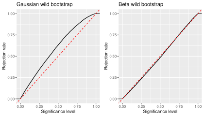
It is easy to see that the conditional law of given the data is , where is the sample covariance matrix: . Hence, the Gaussian wild bootstrap is essentially a feasible version of normal approximation for . Then, it is natural to ask whether the approximation accuracy can be improved by more sophisticated bootstrap methods such as the empirical and non-Gaussian wild bootstraps. In the fixed-dimensional setting, it is well-known that standard bootstrap methods improve the approximation accuracy in the coverage probabilities upon normal approximation only when the statistic of interest is asymptotically pivotal (cf. [35, Chapter 3] and [43, Section 3]). However, despite that and are not asymptotically pivotal in general, numerical experiments suggest that third-moment match bootstrap methods would outperform normal approximation (cf. [24, 21]). To appreciate this, we depict in Fig. 1 the P-P plot for the rejection rate against the nominal significance level when and , where is computed either the Gaussian wild bootstrap or a wild bootstrap with third-moment match. We can clearly see that the latter performance is much better than the former.
Deng & Zhang [24] tried to explain this phenomenon by showing that convergence rates of third-moment match bootstrap approximations have a better dimension dependence, i.e. they achieve and in (1.3). Later, however, it was shown in [36] that the same convergence rate is achieved by normal approximation, i.e. (1.1) holds with and . Chernozhukov et al. [21] have further improved the convergence rate to and for both normal and bootstrap approximations. Meanwhile, if we require to be invertible, it is possible to achieve the Berry–Esseen rate up to a log factor even in the high-dimensional setting. Results in this direction first appeared in Fang & Koike [26], where the following result is obtained when are log-concave:
| (1.4) |
This rate is known to be optimal up to the factor in terms of both and ; see Proposition 1.1 in [26]. This type of results has been further investigated in [44, 39, 23]. In particular, Chernozhukov et al. [23] have obtained the above nearly optimal rate when is bounded. Here, the boundedness condition can be replaced with the sub-exponential condition by a simple truncation argument; see Appendix A. Further, in some situations, the rate is (nearly) attainable even when is (asymptotically) degenerate; see [45, 27, 29]. Nevertheless, all of these improvements are valid for normal approximation and thus do not explain the superior performances of third-moment match bootstrap approximations.
In this paper, we aim to explain the superior performance of bootstrap approximation in high-dimensions using Edgeworth expansion and related techniques. Our first main result shows that, if valid Edgeworth expansions for and are available, then we have
| (1.5) |
provided that is computed by a third-moment match bootstrap method. Thus the coverage error has a better dimension dependence than the optimal normal approximation rate in (1.4). An analogous result holds for but we do not need the third-moment matching condition in this case. The next question is when we have valid Edgeworth expansions in the high-dimensional setting. We answer this question by proving the validity of Edgeworth expansion for when have Stein kernels (cf. Definition 2.1). This also allows us to derive a valid Edgeworth expansion for the wild bootstrap statistic when the weights have Stein kernels. In particular, our results cover the simulation setting for Fig. 1 (cf. Example 2.2). Finally, we construct a second-order accurate critical value in the sense that
| (1.6) |
for some constant . A classical solution to this problem is bootstrapping the studentized version of , but this is impossible in high-dimensions since the sample covariance matrix is degenerate whenever . Instead, we achieve this by Beran [6]’s double bootstrap method, another classical technique to improve the approximation accuracy for non-pivotal statistics. To prove the second-order accuracy of the double bootstrap, we develop an asymptotic expansion formula of in Theorem 3.3. As a byproduct, we find that the wild bootstrap with third moment match is already second-order accurate when and has identical diagonal entries and bounded eigenvalues, revealing the blessing of dimensionality in this context; see Corollary 3.1.
Despite that Edgeworth expansion is a standard tool to analyze the performance of bootstrap in the classical setting (cf. [35]), this approach has not been investigated for the above problem so far. A main reason would be the lack of valid Edgeworth expansion for and in the high-dimensional setting. While asymptotic expansion for statistics of high-dimensional data has been actively studied in multivariate statistics (see [33] for an overview), results developed there seem inapplicable to our problem. One main reason is that and may not have any limit distributions as even after properly scaled. In fact, this is one of the motivations for the development of Chernozhukov–Chetverikov–Kato’s theory. In view of (1.4), we are concerned with Edgeworth expansion of over . In the fixed-dimensional setting, a valid Edgeworth expansion of is conventionally derived from an asymptotic expansion of the characteristic function of via Fourier analysis (see e.g. [7]). Such an argument makes the dimension dependence of the error bound extremely complicated, so it is rarely given explicitly. One exceptional work is Anderson et al. [1], but their proof technique seems to inherently require the condition and thus inapplicable to our setting. In fact, in the high-dimensional setting, the geometry of the set plays a key role to get an improved dimension dependence of error bounds, and it is unclear how to incorporate such information into Fourier analytic arguments. We also mention the recent work by Zhilova [57] who establishes explicit, computable error bounds for where is another sum of independent random vectors and is either the class of balls or half-spaces. However, apart from other technical issues, these error bounds contain terms and cannot be used for second-order analysis.
To circumvent the above issue, we develop valid asymptotic expansions using Stein’s method. The use of Stein’s method for asymptotic expansion was initiated by Barbour [2] who derived an asymptotic expansion of when and is a smooth function. To drop the smoothness of the test function , the so-called Cramér’s condition is usually assumed in the Fourier analytic approach, but it is unknown how to (directly) incorporate Cramér’s condition into Stein’s method based arguments. Instead, we assume that the underlying random vectors have Stein kernels, motivated by the recent development of this approach by Fang & Liu [30] in the univariate case (see Lemma 2.1 ibidem). Apart from the technical difficulty, Cramér’s condition is violated whenever the underlying statistic has a singular covariance matrix. This is unsuitable for application to bootstrap statistics in high-dimensions, so Stein kernels will be a more appropriate tool for our problem (see 2.6).
The remainder of the paper is organized as follows. In Section 2.1, we give the precise form of claim (1.5). In Section 2.2, we develop valid Edgeworth expansions for and in high-dimensions. Then, we study the second-order accuracy of bootstrap approximations for in Section 3: After developing Cornish–Fisher type expansions for and in Section 3.1, we develop an asymptotic expansion formula for in Section 3.2. Based on this result, we show in Section 3.3 that a double wild bootstrap method is second-order accurate. Section 4 contains a small simulation study. Most proofs are collected in Sections 5 and 6. Exceptions are proofs for properties of Stein kernels, which are given in Appendix C. The appendix also contains other additional proofs and auxiliary results.
Notation
Throughout the paper, we assume that has an invertible covariance matrix and denote by the square root of the minimum eigenvalue of . We also set and . Further, denote i.i.d. random variables independent of . They are used to define the wild bootstrap statistic in (1.2). We always assume and . Also, and denote the conditional probability and expectation given the data , respectively. For , denotes the conditional -quantile of given the data, i.e. .
For a vector , we set and . We denote by the all-ones vector in . For , denotes the set of real-valued -dimensional -arrays . In particular, and is the set of matrices. For and , we set . We write for short. When , we also set . In particular, when , is the Euclidean inner product of and which we also write . In addition, we set and Further, for , we define . Finally, we set
Given an -times differentiable function , we set for , where . For , denotes the set of bounded functions with bounded derivatives.
For an invertible matrix , denotes the density of . We write for short, where is the identity matrix. Further, we write for short. denotes the standard normal distribution function. Also, for a distribution function , its (generalized) inverse is defined as We refer to Appendix A.1 in [10] for useful properties of inverse distribution functions.
For a random vector and , we set (recall that is the Euclidean norm). Further, for , we set . For two random vectors and , we write if has the same law as .
We assume whenever we consider an expression containing . A similar convention is applied to .
2 High-dimensional bootstrap and Edgeworth expansion
2.1 Coverage error bounds via Edgeworth expansion
We begin by introducing appropriate (second-order) Edgeworth expansions for and . The former is standard. That is, our Edgeworth expansion for is defined as
The situation is different for the latter. In the low-dimensional setting, a natural bootstrap version of would be obtained by replacing and with their sample counterparts and , respectively. However, when , is always degenerate, so is not well-defined. For this reason, we consider an Edgeworth expansion “around ”. Formally, our Edgeworth expansion for is defined as
where is a constant determined by the construction of . We expect for third moment match bootstrap methods.
Theorem 2.1.
Suppose that there exist constants , and such that
| (2.1) |
and
| (2.2) |
with probability at least . Suppose also that there exists a constant such that
| (2.3) |
Then, there exists a universal constant such that
| (2.4) |
for any , provided that or . Further, with denoting the -quantile of , we have
| (2.5) |
regardless of the values of and .
Remark 2.1.
(a) The sub-exponential assumption (2.3) is imposed just for clarity. It is necessary only for deriving concentration inequalities for terms of (cf. Lemma E.10) and can be replaced by another assumption as soon as such bounds are available.
(b) While Theorem 2.1 is stated for the wild bootstrap, the conclusion remains true for the empirical bootstrap as long as (2.2) is satisfied. However, so far we have no result to ensure (2.2) with a reasonable for the empirical bootstrap in the high-dimensional setting.
In the next subsection we will see that (2.1) and (2.2) hold with and under regularity conditions. Hence we have (1.5) for the third-moment match bootstrap, showing that it could give a better approximation in the coverage probability than the normal approximation. An intuition behind this improvement is as follows. (2.1) and (2.2) imply that is approximately equal to
| (2.6) |
for every . When or , the right hand side can be written as a sum of centered independent random variables, so a standard argument shows that it is of order for a fixed sequence of (cf. Lemmas E.4 and E.10). It turns out that such estimates give an error bound for of essentially the same order. For , it suffices to consider rectangles of the form for some . In this case, the second term on the right hand side of (2.6) always vanishes since is symmetric. Hence we need neither nor .
Remark 2.2 (Estimation of distribution functions).
Deng & Zhang [24] actually focus on the bootstrap estimation error for the distribution function of in the Kolmogorov distance, i.e. . For this problem, there is a theoretical explanation for why bootstrap approximation outperforms normal approximation in the fixed dimensional setting; see [5, Section 2.1] for details and also [43] for a related discussion. In view of the superior performance of bootstrap approximation reported in the simulation study of [24], we may naturally expect that results in [5] could be extended to the high-dimensional setting. The formal development is left to future research.
Remark 2.3.
Theorem 2.1 does not mean that third-moment match bootstraps work with the weaker requirement compared to the normal approximation. This is because we usually need at least to have vanish. It is known that for some high-dimensional linear models, bootstrap for linear contrasts works with a weaker requirement on the model dimension than the normal approximation (see [46]), so it will be interesting to study whether a similar phenomenon occurs for maximum type statistics.
2.2 Valid Edgeworth expansion in high-dimensions
Let us formally define the notion of Stein kernel.
Definition 2.1 (Stein kernel).
Let be a random vector in with . A measurable function is called a Stein kernel for (the law of) if and
| (2.7) |
for any .
The concept of Stein kernel was originally introduced in Stein [55, Lecture VI] for the univariate case. Although its partial multivariate extension dates back to [13], general treatments have started in more recent studies of [51, 41], stemming from the discovery of connection to Malliavin calculus due to Nourdin & Peccati [49] (the so-called Malliavin–Stein method). We refer to [47] for the recent development.
Remark 2.4 (Alternative definition).
Our definition of Stein kernel is taken from [41]. In the literature, the definition of Stein kernel often requires (2.7) to hold with on the both sides replaced by any bounded function with bounded derivatives. Except for the case , this requirement is slightly stronger than ours. Nevertheless, as far as the author knows, this stronger requirement has so far been met by all known constructions of Stein kernels, including all the examples of this paper.
The validity of Edgeworth expansion for is ensured if the summands have Stein kernels:
Theorem 2.2 (Edgeworth expansion for ).
Suppose that has a Stein kernel for every . Suppose also that there exists a constant such that
| (2.8) |
for all and . Further, assume . Then,
| (2.9) |
Remark 2.5.
Here and below, we do not intend to optimize the dependence of bounds on and .
Below we give a few examples satisfying (2.8).
Example 2.1 (Log-concave distribution).
Example 2.2 (Gaussian copula model).
Let be a positive semidefinite symmetric matrix with unit diagonals. Also, for every , let be a non-degenerate probability distribution on (i.e. is not the unit mass at a point), and denote by its distribution function. The Gaussian copula model with parameter matrix and marginal distributions is defined as for , where .
Proposition 2.1 (Stein kernel of Gaussian copula model).
Suppose that there exists a constant such that, for every and any Borel set ,
| (2.10) |
where . Then has a Stein kernel and
for some universal constant .
The maximal constant satisfying (2.10) is called the Cheeger (isoperimetric) constant of . We refer to [9, Theorem 1.3] for a useful equivalent formulation in the univariate case. When is log-concave, then (2.10) is satisfied with by Proposition 4.1 in [8]. Since the gamma distribution with shape parameter is log-concave, Proposition 2.1 shows that the simulated model in the introduction satisfies the assumptions of Theorem 2.2. We can actually show that any gamma distribution has a positive Cheeger constant; see Proposition C.2.
Example 2.3 (Multiplicative perturbation).
Other constructions of multivariate Stein kernels are found in [47, Section 4], although it does not seem straightforward to verify the second condition of (2.8) for them.
Remark 2.6 (Relation to classical conditions).
(a) In the univariate case, if a non-degenerate distribution has a Stein kernel, then it has a non-zero absolutely continuous part; see Proposition C.1. In particular, it must satisfy Cramér’s condition. It is worth mentioning that, while univariate Stein kernels are often investigated in the existence of density in the literature, a non-degenerate distribution without density can have a Stein kernel. A simple example is the law of , where is a Bernoulli variable with success probability and is a standard normal variable independent of . In this case, we can easily check that has a Stein kernel . More interesting examples are given by Example 2.2 since any univariate distribution can be realized as a Gaussian copula model and (2.10) can hold without density; see discussions after [9, Theorem 1.3].
(b) In the multivariate case, a non-degenerate distribution may not satisfy Cramér’s condition even when it has a Stein kernel: A simple example is a multivariate normal distribution with singular covariance matrix. This example is indeed important in the high-dimensional setting when analyzing the Gaussian wild bootstrap.
We turn to Edgeworth expansion for . Its validity is ensured if the weight variables have Stein kernels:
Theorem 2.3 (Edgeworth expansion for ).
Suppose that (2.3) is satisfied. Suppose also that satisfies either of the following conditions:
-
(i)
has a Stein kernel and there exists a constant such that and .
-
(ii)
. We set in this case.
Further, assume . Set . Then we have
| (2.11) |
with probability at least .
We can construct a random variable satisfying Condition (i) and as follows: Let be a random variable following the beta distribution with parameters . Then satisfies (i) by [42, Example 4.9] and Lemma C.1. Also, we have
where and . From this expression, given a positive constant , we have if we set
| (2.12) |
A drawback of Theorem 2.3 is that two-point distributions do not admit Stein kernels (cf. Proposition C.1). In particular, it does not cover Mammen’s wild bootstrap (cf. Eq.(4.1)) examined in the simulation study of [24]. However, the above standardized beta distribution becomes closer to Mammen’s two-point distribution as is closer to 0, and their numerical difference virtually vanishes. Our simulation study shows that the beta wild bootstrap with performs very similarly to Mammen’s one.
3 Second-order accurate approximation
Our next aim is to construct a second-order accurate critical value in the sense that (1.6) holds. To accomplish this, we will develop an asymptotic expansion of the bootstrap coverage probability. Such an expansion is conventionally derived with the help of Cornish–Fisher expansion (cf. Section 3.5.2 in [35]), so we first develop such expansions for and in our setting.
Before starting discussions, we introduce some notation used throughout this section. For , we set . We denote by the density of , where . Note that is a function since is invertible. Finally, we set . By Lemma E.3, is bounded from below by a positive constant depending only on and . By Lemma E.1, is generally bounded by , but we often have as , known as a superconcentration phenomenon (cf. [15]). For example, this is the case when for all and there exists a constant such that for all . This follows from [15, Theorem 9.12].
3.1 Cornish–Fisher expansion
This section develops Cornish–Fisher type expansions for and .
Theorem 3.1 (Cornish–Fisher expansion for ).
Under the assumptions of Theorem 2.2, let be a constant such that . Then, for any , there exist positive constants and depending only on and such that, if
| (3.1) |
then
| (3.2) |
where is the -quantile of and
Theorem 3.2 (Cornish–Fisher expansion for ).
Under the assumptions of Theorem 2.3, let be a constant such that . Then, for any , there exist positive constants and depending only on and such that, if
| (3.3) |
then
| (3.4) |
with probability at least , where
Remark 3.1.
We are not getting valid Cornish–Fisher type expansions for and because it is not straightforward to derive an adequate bound for the second derivative of the quantile function of . Since there is another technical issue to develop asymptotic expansion of (see 3.3), we do not pursue them in this paper.
3.2 Asymptotic expansion of coverage probability
For a matrix , denotes the -dimensional vector obtained by stacking the columns of . For two random vectors and , the random vector will be denoted by for simplicity.
Theorem 3.3 (Asymptotic expansion of bootstrap coverage probability).
Suppose that the assumptions of Theorem 3.2 are satisfied. For every , set and suppose that the -dimensional random vector has a Stein kernel of the form
| (3.5) |
with an -valued function and such that
| (3.6) |
Then, for any , there exist positive constants and depending only on and such that, if (3.3) holds, then
where
Remark 3.2 (Univariate case).
When and , the above asymptotic expansion formula reduces to
These recover the asymptotic expansion formulae for normal and empirical bootstrap coverage probabilities, respectively; see e.g. [43, Eqs.(2)–(3)] (note that when ).
The new assumption in Theorem 3.3 is the existence of a (nice) Stein kernel for . This assumption can be viewed as a counterpart of joint Cramér’s condition for and that is typically imposed to derive a univariate counterpart of Theorem 3.3; see e.g. Eq.(2.54) in [35]. It is natural in this sense, but the verification is not easy in practice. Here, we give one sufficient condition following Mikulincer [48]’s idea of using the Malliavin–Stein method.
Lemma 3.1.
Let be a standard Gaussian vector in . Let be a locally Lipschitz function such that and . Then has a Stein kernel such that
| (3.7) |
for all and . In addition,
| (3.8) |
for any even integer and .
Moreover, if we further assume and , then for , has a Stein kernel of the form (3.5) and satisfies
for all .
Using this lemma, we give a few examples satisfying (LABEL:ass:joint-sk).
Example 3.1 (Uniformly log-concave distribution).
Let . A probability density function is said to be -uniformly log-concave if there exists a log-concave function such that for all . If has an -uniformly log-concave density, there exists a 1-Lipschitz function such that has the same law as with by Caffarelli’s log-concave perturbation theorem (cf. [14, Theorem 11]). Hence has a Stein kernel of the form (3.5) and satisfies (LABEL:ass:joint-sk) with for some universal constant . We remark that results with similar natures to Caffarelli’s theorem are available for other distributions. We refer to [32] and references therein.
Example 3.2 (Gaussian copula model).
Consider the same setting as Example 2.2. Proposition 2.1 can be extended as follows.
Proposition 3.1.
Set . Under the assumptions of Proposition 2.1, has a Stein kernel of the form (3.5) and satisfies (LABEL:ass:joint-sk) with for some universal constant .
Now we discuss implications of Theorem 3.3 to the second-order accuracy of standard bootstrap approximations. An easy consequence is that any wild bootstrap approximation is second-order accurate when as long as satisfies the assumptions in Theorem 2.3. However, simulation results suggest that the choice of would affect the performance even when , so there is still room to investigate.
The following corollary gives a more interesting implication:
Corollary 3.1.
Under the assumptions of Theorem 3.3, suppose additionally that , , and the maximum eigenvalue of is bounded by with some constant . Then there exist a constant depending only on and such that
| (3.9) |
Observe that the second term on the right hand side of (3.9) is divided by . Hence, Corollary 3.1 implies that the third-moment match wild bootstrap is second-order accurate if and has identical diagonal entries and bounded eigenvalues with respect to . This seems to be a new result on the blessing of dimensionality, although too high-dimensionality is harmful due to the first term of the bound.
Remark 3.3.
The proof of Theorem 3.3 relies crucially on the identity for and . We will use this identity to get an Edgeworth expansion for with a sum of independent random variables (see (6.15)), i.e. is again represented as the maximum of a sum of independent random vectors in this case. We note that this argument is inapplicable to .
3.3 Double wild bootstrap
As mentioned in the introduction, the lack of second-order accuracy in standard bootstrap methods is due to the fact that is not asymptotically pivotal. If we knew the distribution function of , say , then would give an (exactly) pivotal statistic. Beran [6] suggested estimating by the bootstrap distribution function and use to construct critical values. This method is called bootstrap prepivoting. Note that can be computed by simulating the conditional law of given the data. To estimate the law of , we use the following nested double wild bootstrap procedure following [6]: Let be i.i.d. variables independent of everything else and such that and . We define the wild bootstrap statistic of as
Then define for , where and is the conditional probability given . We regard as a bootstrap version of and estimate the law of by the conditional law of . Formally, given a significance level , let be the conditional -quantile of given the data. We expect that would be close to . This is formally justified by the following theorem:
Theorem 3.4 (Second-order accuracy of double bootstrap coverage probability).
Under the assumptions of Theorem 3.3, assume further that has a Stein kernel such that . Suppose also that has a Stein kernel and there exists a constant such that and . Further, assume . Then, for any , there exists a constant depending only on and such that
| (3.10) |
The new assumption here is the existence of a bounded Stein kernel for . This assumption is not problematic in practice because beta random variables still work:
Proposition 3.2.
Let be a beta random variable and set . Then has a bounded Stein kernel.
Remark 3.4 (-value).
One can easily check that is equivalent to , where and are the -values of the first and second level bootstraps, respectively. Hence the -value of the double bootstrap method is .
4 Simulation study
This section conducts a small Monte Carlo study to supplement our theoretical findings. We adopt the same simulation design as [24]: We set and generate the data from a Gaussian copula model, i.e. are i.i.d. with the same law as , where is defined as in Example 2.2. The marginal distributions are the gamma distribution with shape parameter 1 and unit scale. As the parameter matrix , we consider two designs: (I) and (II) . Here, the parameter is varied as . We compute the rejection rates and at the 10% significance level based on 20,000 Monte Carlo iterations, where is an estimated 90% quantile of the corresponding statistic using various bootstrap methods. In addition, to assess the performance when the skewness of the data is zero, we also consider the case that , where is an independent copy of . To keep the marginal kurtosis at the same level, we change the shape parameter of the gamma distribution to in this case.
For the bootstrap methods, we consider the empirical bootstrap (EB), wild bootstrap and double wild bootstrap (DB) methods. For the wild bootstrap, we consider the following 4 types of weight variables:
- GB
-
is a standard normal variable.
- MB
-
follows Mammen’s two point distribution [46]:
(4.1) - RB
-
is a Rademacher variable: .
- BB
-
follows the standardized beta distribution with parameters given by (2.12) with .
The double wild bootstrap is implemented with both and generated from the standardized beta distribution with parameters given by (2.12) with . Note that our theoretical results are applicable to only GB, BB and DB. We include EB, MB and RB in our assessment because they are commonly used in the literature. The number of bootstrap replications is set to 499 for the first-level bootstrap and 99 for the second-level bootstrap in DB.
We summarize the simulation results in Tables 1 and 2. First, Table 1 reports empirical rejection rates at the 10% level when the laws of are asymmetric. We find that the difference of performances between GB and BB is largely in line with our Theorem 2.1 except for in Design (I) with : BB performs better than GB for , while they perform similarly for . For in Design (I) with , GB outperforms BB. This phenomenon might be explained as follows: In Design (I), for , has the same law as , where and are independent. Since , is asymptotically normal as in this case. This perhaps imply that behaves as in the classical setting when and are large. Then, it is known that normal approximation typically outperforms bootstrap approximation without studentization in terms of coverage errors; see [43, Section 3] for details. Turning to the performance of DB, it tends to over-reject but outperforms GB and BB in Design (I). The latter is expected since our theory reveals that DB are second-order accurate while GB and BB are generally not. In Design (II), the performances of DB and BB are comparable. This would be because has no large eigenvalues; see Corollary 3.1.
Next, Table 2 reports empirical rejection rates at the 10% level when the laws of are symmetric. Recall that our Theorem 3.3 implies that both GB and BB are second-order accurate (at least) for in this case. Reflecting this fact, GB clearly performs better than the asymmetric case for . The performance of BB is improved in Design (I) but not in Design (II). The latter would be due to the same reasoning as above, i.e. BB is second-order accurate in Design (II) even when the skewness is not zero by Corollary 3.1. By contrast, the performance of DB is not improved. This is not surprising because DB is already second-order accurate in the asymmetric case and the zero skewness condition would not contribute to its performance. When comparing GB and BB, BB still outperforms GB. This may be due to an effect of kurtosis, but we will need higher-order asymptotic expansions for the formal discussion and leave it to future work.
Finally, we briefly discuss the performances of EB, MB and RB. First, EB tends to under-reject and its performance is not pronounced compared to other methods. In fact, we can observe similar phenomena in the simulation results of [24, 21]. Formally, this does not contradict our theory because we have no valid Edgeworth expansion for EB in high-dimensions, although it is unclear whether this is an artifact of our proof strategy. Next, although MB is not covered by our theory, its performance is similar to BB. This is perhaps explained by the fact that their weights are very close numerically. Third, RB performs remarkably well in the symmetric case. This is already observed in the simulation study of [21] who explain this phenomenon by their Theorem 2.3. Another possible explanation is the match of higher moments, but we have no formal theoretical result for this so far.
| EB | GB | MB | RB | BB | DB | ||
| (I) | |||||||
| 0.2 | 0.061 | 0.124 | 0.080 | 0.155 | 0.078 | 0.114 | |
| 0.060 | 0.073 | 0.082 | 0.107 | 0.079 | 0.114 | ||
| 0.8 | 0.071 | 0.090 | 0.072 | 0.093 | 0.071 | 0.101 | |
| 0.091 | 0.091 | 0.097 | 0.099 | 0.097 | 0.100 | ||
| (II) | |||||||
| 0.2 | 0.065 | 0.146 | 0.092 | 0.195 | 0.091 | 0.117 | |
| 0.061 | 0.083 | 0.086 | 0.123 | 0.085 | 0.117 | ||
| 0.8 | 0.069 | 0.139 | 0.089 | 0.177 | 0.088 | 0.113 | |
| 0.062 | 0.079 | 0.084 | 0.113 | 0.083 | 0.112 | ||
| EB | GB | MB | RB | BB | DB | ||
| (I) | |||||||
| 0.2 | 0.065 | 0.076 | 0.083 | 0.100 | 0.082 | 0.114 | |
| 0.058 | 0.067 | 0.082 | 0.099 | 0.082 | 0.113 | ||
| 0.8 | 0.089 | 0.092 | 0.091 | 0.096 | 0.091 | 0.105 | |
| 0.082 | 0.084 | 0.088 | 0.093 | 0.088 | 0.093 | ||
| (II) | |||||||
| 0.2 | 0.062 | 0.071 | 0.085 | 0.101 | 0.084 | 0.114 | |
| 0.056 | 0.068 | 0.084 | 0.104 | 0.083 | 0.119 | ||
| 0.8 | 0.067 | 0.076 | 0.088 | 0.100 | 0.086 | 0.109 | |
| 0.060 | 0.070 | 0.087 | 0.105 | 0.086 | 0.118 | ||
5 Proofs for Section 2
We use the following notation in the remainder of the paper: For two random variables and , we write or if there exists a universal constant such that . Also, given real numbers , we use to denote positive constants, which depend only on and may be different in different expressions.
5.1 Proof of Theorem 2.1
Without loss of generality, we may assume
| (5.1) |
Since , this particularly yields .
Let us prove (2.4). Let be the event on which (2.2) holds. We have by assumption. Also, by (2.1),
| (5.2) |
Next, by Lemma E.4, there exists a universal constant such that
Also, by Lemma E.10, there exists a universal constant such that
for any and
for any . Now we set
For every , recall that we have the decomposition (2.6). Therefore, setting
we have , provided that or .
Set . Also, recall that is the -quantile of for and thus . Then, if , we have on
where . Thus, on ,
This implies on . Hence
Thus . Also, this bound trivially holds if . Meanwhile, if , we have on
where . Observe that
where we used (5.2) for the first inequality. Hence, on ,
Thus on . Hence
Thus and this trivially holds if . Finally, using (5.1) and , we can easily check . All together, we obtain (2.4).
5.2 Proofs of Theorems 2.2 and 2.3
The proofs are based on the following two abstract error bounds for high-dimensional Edgeworth expansion (the latter is used for the Gaussian wild bootstrap):
Theorem 5.1 (Error bound for high-dimensional Edgeworth expansion via Stein kernel).
Let be independent random vectors in with mean 0 and finite variance. Set and . Suppose that has a Stein kernel and satisfies for all . Set , and
| (5.3) |
Then, there exists a universal constant such that for any ,
| (5.4) |
Theorem 5.2 (Refined Gaussian comparison inequality).
Let be a centered Gaussian vector in with covariance matrix . Then, there exists a universal constant such that for any ,
where is defined by (5.3); note that in the present case.
First we prove Theorems 2.2 and 2.3 using the above results. Below we will frequently use the following identity without reference: For any and ,
This follows from the AM-GM inequality.
-
Proof of Theorem 2.2.We apply Theorem 5.1 with . Observe that and that has a Stein kernel satisfying .
Let us bound the quantities appearing in the right hand side of (5.4). First, noting that , we have
Thus, by Lemma E.9 with , and , we obtain
(5.5) where the second inequality follows from . Next, by Lemma E.7 and Lemma E.9 with , and ,
Therefore,
(5.6) where the last inequality follows from . Similarly, we can show that
(5.7) (5.8) In addition, by the Schwarz inequality,
Similarly to the proof of (5.6), we can prove
where the second inequality follows by the assumption . Combining this with (5.5) gives
(5.9) where the second inequality follows by the assumption . Also, by (5.8) and (5.9),
where we used the assumption in the second inequality. All together, we obtain by Theorem 5.1
for any . With , we obtain
Consequently, we obtain the desired result. ∎
-
Proof of Theorem 2.3.First consider Case (i). Set for . We apply Theorem 5.1 with and conditional on the data. Note that, conditional on the data, has a Stein kernel satisfying by Lemma C.1. Therefore, we have
(5.10) where
and
Next, by Lemmas E.9 and E.11, there exists a universal constant such that the event
(5.11) occurs with probability at least . Recall that by assumption. Hence, on , we have
(5.12) and
(5.13) Thus, on ,
(5.14) Meanwhile, for every , we have on
(5.15) Combining this bound with (5.12), we have on
(5.16) Further, by (5.12), (5.15), the construction of and , we have on
(5.17) and
(5.18) Now we bound the right hand side of (5.10) on the event . First, we have
(5.19) where We decompose as
Since
we have on
(5.20) by (5.17). Meanwhile, by Nemirovski’s inequality (cf. Lemma 14.24 in [12]),
Hence we have on
(5.21) by (5.18). Combining (5.19)–(5.21) with (5.14), we obtain
(5.22) Consequently, we have
(5.23) where we used the assumption for the last inequality. Next, we have
(5.24) where the second inequality follows by the AM-GM inequality and (5.16). Similarly, we can prove
(5.25) (5.26) (5.27) (5.28) Also, by (5.27),
(5.29) Further, by the Schwarz inequality, (5.22) and (5.26),
(5.30) Combining (5.10), (5.14), (5.23), (5.26), (5.28)–(5.30) and , we have, on ,
It remains to prove
(5.31) Observe that
(5.32) and
Also, note that . Hence (5.31) follows from (5.12) and (5.15).
Next consider Case (ii). In this case, conditional on the data. Hence, applying Theorem 5.2 and using the bounds (5.12), (5.14) and (5.32), we obtain the desired bound with a simplified argument of the proof for Case (i). ∎
Now we turn to the proof of Theorems 5.1 and 5.2. As usual, the proof starts with a smoothing inequality. We will use the following version.
Lemma 5.1.
Let be a finite measure, a finite signed measure, and a probability measure on . Let be a constant such that Let be a bounded measurable function. Then we have
where
with ,
and denotes the convolution of two finite signed measures.
The proof of this lemma is a straightforward modification of [7, Lemma 11.4] and given in Section B.1, but its statement contains an important difference from the original one: The bound does not contain the positive part of the signed measure . This is important for bounding and in our setting. To bound these quantities, we will use the following anti-concentration inequality. For and , define .
Lemma 5.2.
Let . Then
| (5.33) |
where is a constant depending only on .
-
Proof.See Section B.2. ∎
We will apply Lemma 5.1 with . To bound the quantity , we introduce some notation and lemmas. Given a bounded measurable function and , we define a function as
where . When , can be rewritten as
By this expression, is infinitely differentiable and
| (5.34) |
for any . In particular, . We will use the following lemmas to bound .
Lemma 5.3.
Let be a bounded measurable function and . Then, under the assumptions of Theorem 5.1,
| (5.35) |
Also, under the assumptions of Theorem 5.2,
| (5.36) |
-
Proof.See Section B.3. ∎
Lemma 5.4.
Let with . Then, for any and ,
| (5.37) |
where is a constant depending only on .
-
Proof of Theorem 5.1.We apply Lemma 5.1 to and defined as
Since
we have with . Let with . Then we have and , where we set for any with interpreting if . Hence
and
Further, for each , set
Then we have , , and
Consequently,
Besides, for any and , we have . For each , set
Then we have , , and
Also, observe that and . Hence we conclude
In addition, observe that for any . As a result, Lemma 5.1 gives
Note that for any . Thus, we have by Lemmas E.2 and 5.2
Further, by Lemma 5.4, we have for any
Also, by the AM-GM inequality,
Since
we obtain the desired result by (5.35). ∎
-
Proof of Theorem 5.2.The claim follows by replacing (5.35) with (5.36) in the proof of Theorem 5.1. ∎
6 Proofs for Section 3
Given a random vector , we denote by the distribution function of .
6.1 Proofs of Theorems 3.1 and 3.2
The proofs are based on the following abstract result.
Proposition 6.1 (Abstract Cornish–Fisher type expansion for maximum statistics).
Let . Also, let be a random vector in . Suppose that there exist arrays and a constant such that
| (6.1) |
where Set
Then, there exist positive constants and depending only on such that, if , then
where
First we prove Theorems 3.1 and 3.2 using Proposition 6.1.
-
Proof of Theorem 3.1.First, observe that Lemma E.3 yields
(6.2) Hence, due to (3.1), we may assume
(6.3) Then, we have (2.9) by Theorem 2.2. Also, observe that . Hence, in this setting, and in Proposition 6.1 are bounded as
where we used (6.3) for the second inequality. Combining these bounds with (6.2) and (6.3) gives
Consequently, the desired result follows from Proposition 6.1. ∎
-
Proof of Theorem 3.2.By the same reasoning as in the proof of Theorem 3.1, we may assume
(6.4) Let be the event defined by (5.11). Recall that . Also, by the proof of Theorem 2.3, we have (2.11) on . Further, recall that we have (5.13) and (5.15) on . Hence, on
Consequently, a similar argument to the proof of Theorem 3.1 gives the desired result. ∎
Now we turn to the proof of Proposition 6.1. The proof relies on the following lemma.
Lemma 6.1.
Let be a centered Gaussian vector in . If has a continuous density , then
| (6.5) |
for all . Moreover, if , there exists a universal constant such that
| (6.6) |
for all .
-
Proof.See Appendix D. ∎
Remark 6.1.
Under the first assumption of Lemma 6.1, we can also derive the following Gaussian type isoperimetric inequality for : For all ,
| (6.7) |
where . In fact, by [3, Proposition 5], (6.7) follows once we prove
for any locally Lipschitz function . The latter follows by applying Bobkov’s functional Gaussian isoperimetric inequality to the function (cf. Eq.(2) of [3]). While (6.7) has a better dependence on than (6.5), it is often the case that as already mentioned at the beginning of Section 3, so (6.5) is preferable to (6.7) in terms of the dimension dependence.
-
Proof of Proposition 6.1.Observe that
Hence, by Lemmas E.4 and 5.2, there exists a universal constant such that
(6.8) and
(6.9) for all . Also, for any , we have by (6.1)
(6.10) and
(6.11) Combining these bounds with (6.8) gives Therefore, provide that , we have by the mean value theorem and (6.5)
for some constant depending only on . Thus we obtain
This and (6.9) give
Combining this with (6.10) and (6.11), we obtain
(6.12) Thus, provided that , we have by Taylor’s theorem and (6.6)
for some constant depending only on . Combining this with (6.5), (6.8) and (6.12) gives
Since , this completes the proof. ∎
6.2 Proof of Theorem 3.3
Lemma 6.2.
For any and ,
-
Proof.Let . Then, for any ,
Differentiating the both sides times with respect to and setting , we obtain the desired result. ∎
Lemma 6.3 (Anti-concentration inequality for ).
-
Proof.The claim immediately follows by combining Theorem 2.2 with Lemmas E.2 and 5.2. ∎
-
Proof of Theorem 3.3.By Theorems 3.1 and 3.2, there exist positive constants and depending only on and such that, if (3.3) holds, then we have (3.2) and (3.4) with probability at least . In the sequel we assume (3.3) is satisfied with this and fix arbitrarily. By (6.5) and Lemmas E.4 and E.10
with probability at least . Combining this with (3.2) and (3.4), we have
(6.13) with probability at least , where . This and Lemma 6.3 give
(6.14) where the second inequality follows by (3.3). Now, observe that
(6.15) where
(6.16) Hence we can derive an Edgeworth expansion for by applying Theorem 5.1 with . By Lemma C.1, has a Stein kernel such that , where
We are going to bound the quantities appearing in the right hand side of (5.4). First, by (6.5) and Lemma E.4
(6.17) Hence, by Lemma E.6 and (3.3),
(6.18) and
(6.19) These estimates allow us to prove (5.6)–(5.8) with replaced by in a similar manner to the proof of Theorem 2.2. Further, observe that
Combining these estimates with (6.19), we can also prove (5.5) with replaced by similarly to the proof of Theorem 2.2. All together, we can proceed as in the proof of Theorem 2.2 and then obtain
where
Therefore, in view of Theorem 2.2 and (5.2), it remains to prove
(6.20) (6.21) Let us prove (6.20). By Lemma 5.2,
Also, by Taylor’s theorem and Lemma D.1,
Further, Lemma E.4 and (6.5) yield
(6.22) Combining these three estimates gives (6.20). Next, to prove (6.21), consider the following decomposition:
We can rewrite as
where we used Lemma 6.2 for the last equality. We are going to prove in the last expression can be replaced by . By Lemma 5.2 and (6.17),
Consequently, we deduce
where we also used (3.3) and (6.2) for the last inequality. Meanwhile, by Lemma E.4 and (6.18),
and
All together, we complete the proof. ∎
6.3 Proof of Corollary 3.1
First, replacing by , we may assume without loss of generality. Note that we have under this assumption. Next, set . Note that we have because coincides with the minimum principal minor of of size 2.
We begin by proving the following inequalities for every :
| (6.23) |
The first one is an immediate consequence of Lemma A.6 in [4]. Meanwhile, by Eq.(4.2.9) in [40] (see also Eq.(4.2.1) in [40]), we have for any
Set . Observe that Hence we obtain
Further, observe that . Thus, with , we have by Lemma 10.3 in [11]
| (6.24) |
In addition, by the well-known inequality for all , we deduce . Hence we obtain
Therefore, if the second term on the right hand side is less than , then , so . Hence the second bound in (6.23) follows by (6.24). Otherwise, we have for some constant depending only on and , so the second bound in (6.23) trivially holds with sufficiently large .
Now we turn to the main body of the proof. Since the left hand side of (3.9) is bounded by 1, we may assume (3.3) holds with the constant in Theorem 3.3. Also, we have by (6.5). Thus, the proof completes once we show that
| (6.25) |
for any . Observe that
Thus, by the Schwarz inequality
We have
where the last inequality follows from Lemma E.4. Also,
Therefore, (6.25) follows once we show
| (6.26) |
Below we write for short. Fix arbitrarily. A straightforward computation shows
where . Hence
| (6.27) |
where and . It is well-known that the conditional distribution of given is with and (see e.g. Theorem 1.2.5 in [34]). Therefore,
and
Consequently,
| (6.28) |
Combining (6.27) and (6.28) with (6.23) gives
| (6.29) |
Next, fix arbitrarily. Then we have
where . Hence
Let . Then we have
where is the number of elements in . Hence we obtain
where the third inequality follows from (6.23). Combining this with (6.29) gives (6.26). ∎
6.4 Proof of Theorem 3.4
For , we denote by the -quantile of under .
Lemma 6.4.
Under the assumptions of Theorem 3.4, there exist positive constants and depending only on and such that, if (3.3) holds, then
-
Proof.The proof is basically a straightforward modification of that of Theorem 3.3. We only give a sketch of the proof with emphasis on relatively major changes.
Fix arbitrarily. First, it is not difficult to see that an analogous result to Theorem 3.2 holds for . Thus, by a similar argument to the proof of (6.13), we can find a constant depending only on and and an event satisfying the following conditions:
In the sequel we assume (3.3) is satisfied with the above . Then, by a similar argument to the proof of (LABEL:anti-tstat-applied), we obtain
where and is defined as in (6.16). Since by Markov’s inequality and (iii), we conclude
with probability at least . As in the proof of Theorem 3.3, we derive an Edgeworth expansion for by applying Theorem 5.1 with conditional on the data, where and . Conditional on the data, has a Stein kernel such that
where and . It is not difficult to check that we have the estimates corresponding to (5.24)–(5.27) in the present setting with probability at least by a similar argument to the proof of Theorem 2.3. Meanwhile, by the Schwarz inequality,
and
Observe that . Hence, by (6.17) and Lemma E.10,
with probability at least . Combining these estimates with (5.16) and the argument to prove (5.22), we obtain the estimate corresponding to (5.22) with replaced by with probability at least . All together, we can proceed as in the proof of Theorem 2.3 and then obtain
with probability at least , where
The remaining proof is a minor modification of the proof of (6.21), so we omit the details. ∎
Lemma 6.5.
Under the assumptions of Theorem 3.4, there exists a constant depending only on and such that
| (6.30) |
for any and .
-
Proof of Theorem 3.4.Denote by and the constants and in Theorem 3.3, respectively. Also, denote by and the constants and in Lemma 6.4, respectively. Since the left hand side of (3.10) is bounded by 1, we may assume (3.3) holds with without loss of generality. Then, for each , the event
occurs with probability at least . Meanwhile, by (3.3), (6.5) and Lemmas E.4 and E.9, there exists a constant depending only on such that the event
occurs with probability at least and
(6.31) Further, let be the constant in Lemma 6.5. Set
Since the left hand side of (3.10) is bounded by 1, we may assume without loss of generality
(6.32) Now fix arbitrarily. Set and . By (6.31) and (6.32), . Hence, on ,
where the last inequality follows from (6.30) and (6.31). This yields on . Hence
(6.33) where the second inequality is by Theorem 3.3, the third by and the fourth by (6.30) and (6.31). Similarly, with and , we have on
Hence on . Therefore, a similar argument to (6.33) yields
Combining this and (6.33) gives the desired result. ∎
Appendix
Appendix A Nearly optimal high-dimensional CLT under the sub-exponential condition
Theorem A.1.
Set for . Suppose that there exists a constant such that and . Then there exists a universal constant such that
| (A.1) |
where and is the minimum eigenvalue of the correlation matrix of .
-
Proof.As announced, the proof is a combination of [23, Theorem 2.1] and a simple truncation argument used in [36, Section 5.2] and [29, Section 4.3]. Denote by the left hand side of (A.1). Considering instead of , we may assume for all without loss of generality. Further, since , we may also assume
(A.2) Next, let . For and , define and set and . Note that . Then, by a similar argument to the proof of Eq.(4.19) in [29], we obtain
where . Since , it remains to prove
(A.3) We prove this bound by applying Theorem 2.1 in [23] with . This gives
(A.4) where . By (A.2) and ,
and
Further, by Eq.(26) in [36] and (A.2),
Appendix B Proofs of the auxiliary results in Section 5.2
B.1 Proof of Lemma 5.1
As already mentioned, the proof is a straightforward modification of [7, Lemma 11.4]. Let
Assume first that
| (B.1) |
Then, given any , there exists a vector such that In this case, we have
and
Consequently, we obtain
Letting , we obtain the desired result. If instead of (B.1) we have
then, given any , we can find such that Now look at (instead of ) and note that and
for every . Proceeding exactly as above, we obtain
Thus we complete the proof. ∎
B.2 Proof of Lemma 5.2
We divide the proof into four steps.
Step 1. First we reduce the proof to the case . Let and . Then, for any , and , we have
Differentiating the both sides times with respect to and then setting , we obtain
Observe that and . Hence
Therefore, the claim for general follows from that for .
Step 2. In this and the next steps, we show that the quantity inside on the left hand side of (5.33) can be replaced by a weighted surface integral of over the boundary of . Note that an analogous result for the case is standard in the literature; see e.g. Proposition 1.1 in [53]. For , and , set
In this step, we prove
Take arbitrarily. For any and , observe that and is the disjoint union of and . This implies that
and thus . Repeating this procedure gives for . Hence
Since is arbitrary, we obtain the desired result.
Step 3. For any Borel set , and , define
where and means that is omitted. Then, for and , set
where . In this step, we prove
Fix , and . For , we set
Then, and this is a disjoint union. Hence we have
One can easily check that
Hence we obtain
For any , observe that is the disjoint union of
and
Therefore, we have
Thus,
This gives the desired result.
Step 4. It remains to prove
| (B.2) |
We first note that if is an orthant, i.e. for all , then (B.2) immediately follows from the fundamental theorem of calculus and Lemma E.4. In fact, we have in this case
for any and . In the following we show that the proof is essentially reduced to this case by a similar argument to the proof of [26, Lemma 2.2]. For every , set
Also, for any , let
Then, for any , and , we have
For each , the cardinality of the set is bounded by a constant depending only on . Therefore, to prove (B.2), it suffices to show that
| (B.3) |
for any (fixed) , , and , .
To prove (B.3), we introduce additional notation. For a non-negative integer , denotes the -th Hermite polynomial, i.e. . When , we set . Also, we denote by the maximum root of . For example, . Finally, set and define
The function satisfies the following properties by Lemma A.1 in [26]:
| (B.4) | |||
| (B.5) |
Now, we fix and for a while. Set
Then we have
where the last inequality follows from (B.5) and the identity . Set for . Then we have Combining this with (B.4) gives
Now, observe that for any and by construction. Hence, if ,
where we used the identity . On the other hand, if ,
Consequently,
With , we can rewrite the right hand side of the above inequality as
This quantity is bounded by
| (B.6) |
For any , observe that
Therefore, by Lemma E.4, the quantity in (B.6) is bounded by . This gives (B.3). ∎
B.3 Proof of Lemma 5.3
The proof of (5.35) is an almost straightforward multi-dimensional extension of that of [30, Lemma 2.1], and the proof of (5.36) is its simplification. The following lemma will play a key role in our argument.
Lemma B.1.
Let be a centered random vector in . Suppose that has a Stein kernel such that . Then, for any ,
-
Proof.For every , define a function as
For and , we have
Hence we obtain
The second term on the last line is equal to . To evaluate the first term, define a function as , . Then, using the relation , one can easily verify for all . As a result,
where the second equality follows from the definition of Stein kernel. Combining these identities gives the desired result. ∎
-
Proof of Lemma 5.3.First we prove (5.35). Without loss of generality, we may assume and are independent. Also, it suffices to prove the claim when . To see this, let and . One can easily check that and . Since , the general case follows by applying the claim to and .
Set for every . Then we have and . Therefore, by the fundamental theorem of calculus, we obtain
By the multivariate Stein identity,
Also, since is a Stein kernel for , we have
Consequently,
(B.7) Next, for , by the fundamental theorem of calculus again, we have
Since is independent of , we have by the multivariate Stein identity
Meanwhile, we rewrite as
where . By Lemma B.1, the second term on the last line can be rewritten as
Further, for , since is a Stein kernel for and is independent of and , we have
Hence
Consequently, we conclude
(B.8) Fix and . By the fundamental theorem of calculus and multivariate Stein identity again, we have
We rewrite as
For , is independent of and , so we obtain by the definition of Stein kernel
Hence,
Overall, we conclude
(B.9) Further, note that we have by integration by parts
for any . Hence
and
Consequently,
(B.10) Finally, observe that
(B.11)
Appendix C Properties of Stein kernel
C.1 Basic properties
Lemma C.1.
Let be a random vector in with a Stein kernel . Then, for any and , has a Stein kernel given by .
-
Proof.Straightforward from the definition of Stein kernel. ∎
Proposition C.1.
Let be a centered random variable having a Stein kernel . Then a.s. Moreover, if , then the event occurs with a positive probability and the conditional law of given is absolutely continuous. In particular, the law of has a non-zero absolutely continuous part.
-
Proof.The asserted claims are shown by essentially the same arguments as those in the proofs of [50, Proposition 2.9.4] and [50, Theorem 10.1.1]. We give the details for the sake of completeness.
Let be a bounded Borel subset of . First we prove
(C.1) Consider a Borel measure on given by , where is the law of and is the Lebesgue measure on . Then we have for any compact set . Hence is regular by Theorem 2.18 in [54]. Also, note that by the boundedness of . Therefore, by Lusin’s theorem (see Theorem 2.24 in [54]), for every , there exists a compactly supported continuous function such that . Now define a function as , . Then is a bounded function with , so by the definition of Stein kernel. Since by construction, converges to the quantity on the left hand side of (C.1) as . Meanwhile, since a.s. as by construction, the dominated convergence theorem gives as . So we obtain (C.1).
Let us prove the first claim. Observe that for all . Hence by (C.1). By the dominated convergence theorem, this is still true even if is unbounded. Hence a.s.
It remains to prove the second claim. First, if a.s., then (C.1) implies a.s. (recall the above argument). Taking for some gives a.s. Letting , we obtain a.s. By contraposition, means . Next, if the Lebesgue measure of is zero, then by (C.1). Since , we obtain a.s. Since on , this implies a.s. Hence . This implies that the conditional law of given is absolutely continuous. ∎
C.2 Existence results
C.2.1 Proof of Lemma 3.1
The proof uses the Malliavin–Stein method. We refer to [50, Chapter 2] for undefined notation and concepts used below.
Let be the Hilbert space equipped with the canonical inner product. Consider an isonormal Gaussian process over given by , . We consider Malliavin calculus with respect to . First, approximating by a Lipschitz function and applying Proposition 2.3.8 in [50] and Lemma 1.2.3 in [52], we obtain and for every . Therefore, by Proposition 3.7 in [51], the map defined by for and gives a Stein kernel for . For any and , we have
where the first inequality is by the Jensen and Schwarz inequalities and the second by Lemma 5.3.7 in [50]. If is an even integer, we also have by Lemma 5.3.7 in [50]. Since for each , this completes the first part of the proof. The second part can be shown in a similar way and thus we omit it. ∎
C.2.2 Proof of Propositions 2.1 and 3.1
Denote by the -th row vector of . Then has the same law as with . Hence we may assume is of the form with defined as for and . To apply Lemma 3.1, we need to prove are locally Lipschitz and compute its gradient. To see this, we note that is absolutely continuous and satisfies a.e. by (2.10). This follows from arguments in Section 5.3 of [10] (see also Propositions A.17 and A.19 in [10]). Consequently, is locally Lipschitz. This implies is locally Lipschitz since is Lipschitz, and its gradient is given by a.e. Since , we obtain
where the last inequality follows by Birnbaum’s inequality. Hence . Combining this with Lemmas 3.1 and E.5 gives the desired results. ∎
C.2.3 Cheeger constant of the gamma distribution
Proposition C.2.
Any gamma distribution has a positive Cheeger constant.
-
Proof.Let be the gamma distribution with shape and rate . If , then is log-concave, so the claim follows by Proposition 4.1 in [8]. When , the density of satisfies for every . Hence, in view of Theorem 1.3 in [9], it suffices to prove , where is the distribution function of . Since
we have by L’Hôpital’s rule . This completes the proof. ∎
C.2.4 Proof of Proposition 3.2
Lemma C.2 (Gaussian type isoperimetric inequality for the beta distribution).
Let and be the density and distribution function of the beta distribution with parameters , respectively. Then there exists a constant such that for all .
-
Proof.Since for any , it suffices to prove
By symmetry it is enough to prove the former. When , while , so the claim is obvious. When , by L’Hôpital’s rule, it suffices to prove
First, observe that for any . Hence for any . Next, by the well-known inequality for all , we deduce for all . Since and for all , we conclude . This gives the desired result. ∎
-
Proof of Proposition 3.2.Let be the distribution function of . Then with . Hence, in view of Lemmas 3.1 and C.1, it suffices to show that is bounded. This immediately follows from Lemma C.2. ∎
Appendix D Proof of Lemma 6.1
Lemma D.1.
There exists a universal constant such that .
-
Proof.Observe that
for all . Differentiating this equation twice with respect to gives
Hence the desired result follows from Lemma E.4. ∎
-
Proof of Lemma 6.1.Let us prove (6.5). We write and for short. First we consider the case . Since the function is convex, is concave by Corollary A.2.9 in [56]. Hence, for any ,
Let with a positive constant specified later. Then,
Thus, we need to choose so that has an appropriate lower bound. Noting , we have
where we used the following inequality for the last bound: For any random variable and its median , . Thus, letting we obtain . Consequently,
(D.1) Also, by the fundamental theorem of calculus,
(D.2) where the last inequality holds because is decreasing on . Combining (D.1) with (D.2) gives (6.5).
Next consider the case . Since the function is increasing and concave, is concave. Hence is non-increasing. Thus we obtain
where the last inequality follows from (6.5) for which was already proved in the above.
Appendix E Technical tools
E.1 Inequalities related to multivariate normal distributions
Let be a centered Gaussian vector in . Set and .
Lemma E.1.
and .
Lemma E.2 (Nazarov’s inequality).
If , then for any and ,
-
Proof.See [20, Theorem 1]. ∎
Lemma E.3.
There exists a universal constant such that .
-
Proof.By a straightforward modification of the proof of Theorem 1.8 in [25], we can prove
for some universal constant . In fact, this follows by applying the arguments in the proof of Theorem 1.8 in [25] to with when (Lemma 2.2 in [25] is applied with ). Then, since by Lemma E.1, we obtain the desired result. ∎
Lemma E.4 (Anderson–Hall–Titterington’s bound).
For any ,
where is a constant depending only on .
-
Proof.Let and . Then, for any and , we have
Differentiating the both sides times with respect to and then setting , we obtain
Hence
where the last inequality follows by Lemma 2.2 in [26] because . ∎
E.2 Inequalities related to sub-Weibull norms
Lemma E.5.
Let be a random variable. Suppose that there is a constant such that for all . Then .
-
Proof.See Lemma A.5 in [37]. ∎
Lemma E.6.
For any , there exists a constant depending only on such that
for any random variables .
-
Proof.This follows from Lemma C.2 in [16] and the triangle inequality for the Orlicz norm associated with a convex function. ∎
Lemma E.7.
Let be two random variables such that for some . Then we have where is defined by the equation .
-
Proof.See [38, Proposition D.2]. ∎
Lemma E.8.
Let be independent random variables such that for some and . Then, there is a constant depending only on such that, for any ,
-
Proof.See Lemma 2.1 in [28]. ∎
Lemma E.9.
Let be independent random vectors in . Suppose that there exist constants and such that . Then, there exists a constant depending only on such that
| (E.1) |
for any and
| (E.2) |
for any .
Lemma E.10.
Lemma E.11.
Acknowledgments
The author thanks Xiao Fang and Ryo Imai for valuable discussions about the subject of this paper. This work was partly supported by JST CREST Grant Number JPMJCR2115 and JSPS KAKENHI Grant Numbers JP22H00834, JP22H00889, JP22H01139, JP24K14848.
References
- Anderson et al. [1998] Anderson, N. H., Hall, P. & Titterington, D. (1998). Edgeworth expansions in very-high-dimensional problems. J. Statist. Plann. Inference 70, 1–18.
- Barbour [1986] Barbour, A. (1986). Asymptotic expansions based on smooth functions in the central limit theorem. Probab. Theory Relat. Fields 72, 289–303.
- Barthe & Maurey [2000] Barthe, F. & Maurey, B. (2000). Some remarks on isoperimetry of Gaussian type. Ann. Inst. Henri Poincaré Probab. Stat. 36, 419–434.
- Belloni et al. [2018] Belloni, A., Chernozhukov, V., Chetverikov, D., Hansen, C. & Kato, K. (2018). High-dimensional econometrics and regularized GMM. Working paper. arXiv: 1806.01888.
- Beran [1982] Beran, R. (1982). Estimated sampling distributions: The bootstrap and competitors. Ann. Statist. 10, 212–225.
- Beran [1988] Beran, R. (1988). Prepivoting test statistics: A bootstrap view of asymptotic refinements. J. Amer. Statist. Assoc. 83, 687–697.
- Bhattacharya & Rao [2010] Bhattacharya, R. N. & Rao, R. R. (2010). Normal approximation and asymptotic expansions. SIAM.
- Bobkov [1999] Bobkov, S. G. (1999). Isoperimetric and analytic inequalities for log-concave probability measures. Ann. Probab. 27, 1903–1921.
- Bobkov & Houdré [1997] Bobkov, S. G. & Houdré, C. (1997). Isoperimetric constants for product probability measures. Ann. Probab. 25, 184–205.
- Bobkov & Ledoux [2019] Bobkov, S. G. & Ledoux, M. (2019). One-dimensional empirical measures, order statistics, and Kantorovich transport distances, vol. 261 of Memoirs of the American Mathematical Society. American Mathematical Society.
- Boucheron et al. [2013] Boucheron, S., Lugosi, G. & Massart, P. (2013). Concentration inequalities: A nonasymptotic theory of independence. Oxford University Press.
- Bühlmann & van de Geer [2011] Bühlmann, P. & van de Geer, S. (2011). Statistics for high-dimensional data. Springer.
- Cacoullos & Papathanasiou [1992] Cacoullos, T. & Papathanasiou, V. (1992). Lower variance bounds and a new proof of the central limit theorem. J. Multivariate Anal. 43, 173–184.
- Caffarelli [2000] Caffarelli, L. A. (2000). Monotonicity properties of optimal transportation and the FKG and related inequalities. Comm. Math. Phys. 214, 547–563.
- Chatterjee [2014] Chatterjee, S. (2014). Superconcentration and related topics. Springer.
- Chen & Kato [2019] Chen, X. & Kato, K. (2019). Randomized incomplete -statistics in high dimensions. Ann. Statist. 47, 3127–3156.
- Chernozhukov et al. [2013] Chernozhukov, V., Chetverikov, D. & Kato, K. (2013). Gaussian approximations and multiplier bootstrap for maxima of sums of high-dimensional random vectors. Ann. Statist. 41, 2786–2819.
- Chernozhukov et al. [2015] Chernozhukov, V., Chetverikov, D. & Kato, K. (2015). Comparison and anti-concentration bounds for maxima of Gaussian random vectors. Probab. Theory Related Fields 162, 47–70.
- Chernozhukov et al. [2017a] Chernozhukov, V., Chetverikov, D. & Kato, K. (2017a). Central limit theorems and bootstrap in high dimensions. Ann. Probab. 45, 2309–2353.
- Chernozhukov et al. [2017b] Chernozhukov, V., Chetverikov, D. & Kato, K. (2017b). Detailed proof of Nazarov’s inequality. Unpublished paper. arXiv: 1711.10696.
- Chernozhukov et al. [2022] Chernozhukov, V., Chetverikov, D., Kato, K. & Koike, Y. (2022). Improved central limit theorem and bootstrap approximation in high dimensions. Ann. Statist. 50, 2562–2586.
- Chernozhukov et al. [2023a] Chernozhukov, V., Chetverikov, D., Kato, K. & Koike, Y. (2023a). High-dimensional data bootstrap. Annu. Rev. Stat. Appl. 10, 427–449.
- Chernozhukov et al. [2023b] Chernozhukov, V., Chetverikov, D. & Koike, Y. (2023b). Nearly optimal central limit theorem and bootstrap approximations in high dimensions. Ann. Appl. Probab. 33, 2374–2425.
- Deng & Zhang [2020] Deng, H. & Zhang, C.-H. (2020). Beyond Gaussian approximation: Bootstrap for maxima of sums of independent random vectors. Ann. Statist. 48, 3643–3671.
- Ding et al. [2015] Ding, J., Eldan, R. & Zhai, A. (2015). On multiple peaks and moderate deviations for the supremum of a Gaussian field. Ann. Probab. 43, 3468–3493.
- Fang & Koike [2021] Fang, X. & Koike, Y. (2021). High-dimensional central limit theorems by Stein’s method. Ann. Appl. Probab. 31, 1660–1686.
- Fang & Koike [2022] Fang, X. & Koike, Y. (2022). Sharp high-dimensional central limit theorems for log-concave distributions. Ann. Inst. Henri Poincaré Probab. Stat. (forthcoming). Working paper is available at arXiv: 2207.14536.
- Fang & Koike [2023] Fang, X. & Koike, Y. (2023). From -Wasserstein bounds to moderate deviations. Electron. J. Probab. 28, 1–52.
- Fang et al. [2023] Fang, X., Koike, Y., Liu, S.-H. & Zhao, Y.-K. (2023). High-dimensional central limit theorems by Stein’s method in the degenerate case. Working paper. arXiv: 2305.17365v1.
- Fang & Liu [2022] Fang, X. & Liu, S.-H. (2022). Edgeworth expansion by Stein’s method. Working paper. arXiv: 2211.04174.
- Fathi [2019] Fathi, M. (2019). Stein kernels and moment maps. Ann. Probab. 47, 2172–2185.
- Fathi et al. [2024] Fathi, M., Mikulincer, D. & Shenfeld, Y. (2024). Transportation onto log-Lipschitz perturbations. Calc. Var. Partial Differential Equations 63, 61.
- Fujikoshi & Ulyanov [2020] Fujikoshi, Y. & Ulyanov, V. V. (2020). Non-asymptotic analysis of approximations for multivariate statistics. Springer.
- Fujikoshi et al. [2010] Fujikoshi, Y., Ulyanov, V. V. & Shimizu, R. (2010). Multivariate statistics. Wiley.
- Hall [1992] Hall, P. (1992). The bootstrap and Edgeworth expansion. Springer.
- Koike [2021] Koike, Y. (2021). Notes on the dimension dependence in high-dimensional central limit theorems for hyperrectangles. Jpn. J. Stat. Data Sci. 4, 643–696.
- Koike [2023] Koike, Y. (2023). High-dimensional central limit theorems for homogeneous sums. J. Theoret. Probab. 36, 1–45.
- Kuchibhotla & Chakrabortty [2022] Kuchibhotla, A. K. & Chakrabortty, A. (2022). Moving beyond sub-Gaussianity in high-dimensional statistics: Applications in covariance estimation and linear regression. Inf. Inference 11, 1389–1456.
- Kuchibhotla & Rinaldo [2020] Kuchibhotla, A. K. & Rinaldo, A. (2020). High-dimensional CLT for sums of non-degenerate random vectors: -rate. Working paper. arXiv: 2009.13673.
- Leadbetter et al. [1983] Leadbetter, M. R., Lindgren, G. & Rootzén, H. (1983). Extremes and related properties of random sequences and processes. Springer.
- Ledoux et al. [2015] Ledoux, M., Nourdin, I. & Peccati, G. (2015). Stein’s method, logarithmic Sobolev and transport inequalities. Geom. Funct. Anal. 25, 256–306.
- Ley et al. [2017] Ley, C., Reinert, G. & Swan, Y. (2017). Stein’s method for comparison of univariate distributions. Probab. Surv. 14, 1–52.
- Liu & Singh [1987] Liu, R. Y. & Singh, K. (1987). On a partial correction by the bootstrap. Ann. Statist. 15, 1713–1718.
- Lopes [2022] Lopes, M. E. (2022). Central limit theorem and bootstrap approximation in high dimensions with near rates. Ann. Statist. 50, 2492–2513.
- Lopes et al. [2020] Lopes, M. E., Lin, Z. & Müller, H.-G. (2020). Bootstrapping max statistics in high dimensions: Near-parametric rates under weak variance decay and application to functional and multinomial data. Ann. Statist. 48, 1214–1229.
- Mammen [1993] Mammen, E. (1993). Bootstrap and wild bootstrap for high dimensional linear models. Ann. Statist. 21, 255–285.
- Mijoule et al. [2023] Mijoule, G., Raič, M., Reinert, G. & Swan, Y. (2023). Stein’s density method for multivariate continuous distributions. Electron. J. Probab. 28, 1–40.
- Mikulincer [2022] Mikulincer, D. (2022). A CLT in Stein’s distance for generalized Wishart matrices and higher-order tensors. Int. Math. Res. Not. IMRN 2022, 7839–7872.
- Nourdin & Peccati [2009] Nourdin, I. & Peccati, G. (2009). Stein’s method on Wiener chaos. Probab. Theory Related Fields 145, 75–118.
- Nourdin & Peccati [2012] Nourdin, I. & Peccati, G. (2012). Normal approximations with Malliavin calculus: From Stein’s method to universality. Cambridge University Press.
- Nourdin et al. [2014] Nourdin, I., Peccati, G. & Swan, Y. (2014). Entropy and the fourth moment phenomenon. J. Funct. Anal. 266, 3170–3207.
- Nualart [2006] Nualart, D. (2006). The Malliavin calculus and related topics. Springer, 2nd edn.
- Raič [2019] Raič, M. (2019). A multivariate Berry–Esseen theorem with explicit constants. Bernoulli 25, 2824–2853.
- Rudin [1987] Rudin, W. (1987). Real and complex analysis. McGraw-Hill, 3rd edn.
- Stein [1986] Stein, C. (1986). Approximate computation of expectations. Institute of Mathematical Statistics.
- van der Vaart & Wellner [2023] van der Vaart, A. W. & Wellner, J. A. (2023). Weak convergence and empirical processes. Springer, 2nd edn.
- Zhilova [2022] Zhilova, M. (2022). New Edgeworth-type expansions with finite sample guarantees. Ann. Statist. 50, 2545–2561.