Long-time asymptotics of the Tzitzéica equation on the line

Abstract.

In this paper, the renowned Riemann-Hilbert method is employed to investigate the initial value problem of Tzitzéica equation on the line. Initially, our analysis focuses on elucidating the properties of two reflection coefficients, which are determined by the initial values. Subsequently, leveraging these reflection coefficients, we construct a Riemann-Hilbert problem that is a powerful tool to articulate the solution of the Tzitzéica equation. Finally, the nonlinear steepest descent method is applied to the oscillatory Riemann-Hilbert problem, which enables us to delineate the long-time asymptotic behaviors of solutions to the Tzitzéica equation across various regions. Moreover, it is shown that the leading-order terms of asymptotic formulas match well with direct numerical simulations.

1. Introduction

In a seminal series of papers spanning from 1907 to 1910, the distinguished Romanian geometer Tzitzéica [38] embarked on a pioneering investigation into a unique class of hyperbolic surfaces with non-degenerate second fundamental form in the Euclidean three-space. Tzitzéica found that the ratio $I=K/d^{4}$ (here $K$ is Gauss curvature and $d$ is the Euclidean distance from a fixed point to tangent plane) is constant under equiaffine transformations of Euclidean three-space, thus people called a surface for which $I$ is invariant as Tzitzéica surface [31]. Such surface is known as proper affine sphere in affine geometry because the affine distance from the origin is non-zero constant [28]. The Gauss-Codazzi equations for indefinite proper affine sphere with Blaschke metric $h=2e^{u}dXdT$ in isothermal coordinates and negative affine mean curvature are described by a nonlinear wave equation, which is now known as Tzitzéica equation

$$u_{X,T}=e^{u}-e^{-2u},$$ (1.1)

where $u$ represents a real-valued function. In the context of integrable systems, it had been shown by Mikhailov [35] that Tzitzéica equation (1.1) is a reduction of periodic two dimensional Toda lattice of type $A_{2}^{(2)}$

$$u_{n,X,T}=e^{u_{n}-u_{n-1}}-e^{u_{n+1}-u_{n}},$$

of period three under the constraint $u_{1}=u,u_{2}=-u$ and $u_{3}=0,$ which coincides with the affine root system.

By introducing “light-cone” coordinates $(x,t)$, defined as

$$x=X+T,\quad t=T-X,$$

the Tzitzéica equation (1.1) is transformed into

$$u_{tt}-u_{xx}=e^{-2u}-e^{u}.$$ (1.2)

This groundbreaking equation has been rediscovered in an array of mathematical and physical contexts, underscoring its significance and versatility. The wonderful work of Dodd and Bullough marked the identification of two nontrivial conservation laws associated with this equation [22]. Subsequently, the analytical efforts of Zhiber and Shabat [44] illuminated the existence of an infinite Lie-Bäcklund group linked to the equation, further enriching its theoretical framework. The Tzitzéica equation also demonstrates profound connections with the two-dimensional Toda chain, revealing synergies with statistical $\mathbb{Z}_{N}$ symmetric models [23]. Occasionally, this leads to its alternative designation as the Bullough-Dodd-Zhiber-Shabat equation in honor of these scholars.

Mikharov’s discovery of the Lax pair for the equation (1.2) [35] has paved new paths for exploring various exact solutions, including soliton, finite gap solutions, and algebro-geometric solutions, etc. [7, 18, 30, 40]. The integrable properties of this equation, such as soliton solutions, conservation laws, symmetries, Bäcklund transformations, Darboux transformations, and beyond, have garnered widespread academic interest [1, 32, 18, 37, 7, 36, 46]. This comprehensive body of research has significantly deepened our understanding of the Tzitzéica equation, as evidenced by the extensive literature on these topics.

The well-posedness of the Tzitzéica equation is a significant topic in the study of integrable systems and nonlinear partial differential equations. This involves examining the existence, uniqueness, and continuous dependence of solutions on initial data. In 2017, Jevnikar and Yang took an analytical approach to explore the Tzitzéica equation in elliptic form, focusing on the occurrence of blow-up phenomena and conditions for solution existence [29]. To the best of our knowledge, no precedent exists in the literature for the well-posedness analysis of the Tzitzéica equation as presented herein. Through this work, we endeavor to elucidate the connection between the solution of equation (1.2) and the Riemann-Hilbert problem, thereby charting a new course for the examination of well-posedness of this equation.

In this paper, we delve into the long-time asymptotic behavior of solitonless solutions of the Tzitzéica equation (1.2), with a particular emphasis on initial data confined to the Schwartz class, which is presented below

$$\begin{cases}u_{tt}-u_{xx}=e^{-2u}-e^{u},\\ u(x,0)=u_{0}(x)\in\mathcal{S}({\mathbb{R}}),\quad u_{t}(x,0)=u_{1}(x)\in\mathcal{S}({\mathbb{R}}).\end{cases}$$ (1.3)

Our investigation commences with a comprehensive examination of both the direct and inverse problems inherent to a third-order spectral problem [2, 3]. This examination facilitates the development of an advanced Inverse Scattering Transform (IST) technique [43], specifically tailored for the initial value problem at hand. Through the IST framework, we are able to articulate a solution for the Tzitzéica equation, encapsulated within the mathematical construct of a $3\times 3$-matrix Riemann-Hilbert problem. Furthermore, our research adopts the Deift-Zhou nonlinear steepest descent method to effectively tackle the complexities associated with Riemann-Hilbert problems. This method, originally introduced by Deift and Zhou in 1993 [21] and subsequently generalized by Lenells [34], serves as a pivotal framework within our analysis. Leveraging this approach, we succeed in deriving asymptotic formulas that shed light on the asymptotic behaviors of solutions. For the sake of analytical clarity and simplification, our study meticulously restricts its focus to initial data categorized under the Schwartz class space $\mathcal{S}({\mathbb{R}})$.

The Riemann-Hilbert method has proven to be a powerful analytical tool, influencing various mathematical domains including integrable systems, random matrices, and orthogonal polynomials [19]. Remarkable progress has been made in understanding the long-time asymptotic behaviors of solutions to integrable equations with higher-order Lax pairs, in which the inverse spectral theory of integrable systems of Gelfand-Dickey type with three-order Lax pairs have been well developed and widely studied by Lenells et al [8]. Other notable examples include the Degasperis-Procesi equation [4, 5], both the “good” and “bad” Boussinesq equations [13, 12, 11, 15, 14, 10, 20], the Lenells equation [9], and so on [6, 17, 24, 25, 26, 39, 41, 42]. This evolution highlights the method’s adaptability and its pivotal role in advancing mathematical analysis.

The manuscript is organized as follows: the main results of this work are proposed in Section 2; in Section 3, starting with the Lax pair associated with the Tzitzéica equation, we offer a comprehensive spectral analysis that culminates in the completion of the proof for Theorem 2.5; finally, Section 4 is dedicated to the proof of Theorem 2.7, which articulates the long-time asymptotic behaviors of the solution to the Tzitzéica equation (1.2).

2. Main Results

This section lists the main results of the present work. For the initial value problem (1.3), direct scattering analysis shows that one can define the scattering matrices $s(\lambda)=(s_{ij}(\lambda))_{3\times 3}$ and $s^{A}(\lambda)=(s^{A}_{ij}(\lambda))_{3\times 3}$ in (3.13) and (3.14) below, respectively. With these scattering data in mind, this paper delineates its core contributions through the formulation and proof of three main theorems, which emerge from a foundational theoretical framework, predicated on a series of basic assumptions. Below, we outline these assumptions, which are essential for the derivation of our main results:

Assumption 2.1.

For the initial value problem (1.3), assume for $\lambda\in\bar{D}_{1}\setminus\{0\}$ and $\lambda\in\bar{D}_{4}\setminus\{0\}$, respectively, that the elements $s_{11}(\lambda)$ and $s_{11}^{A}(\lambda)$ are nonzero. That is, we suppose there don’t exist solitons in problem (1.3).

The subsequent discussion will elucidate the rationality of the aforementioned assumption, demonstrating its validity by selecting a specific initial value followed by numerical calculations.

Our first result reveals the characteristics of two spectral functions, denoted as $r_{1}(\lambda)$ and $r_{2}(\lambda)$. These functions are interpreted as the reflection coefficients associated with the equation (1.2), determined by the initial conditions of the system. Furthermore, $r_{1}(\lambda)$ and $r_{2}(\lambda)$ are conceptualized as the nonlinear Fourier transform of the initial data. The properties of these spectral functions are crucial for formulating the Riemann-Hilbert (RH) problem and, subsequently, for the accurate reconstruction of the solution to equation (1.3) from the Riemann-Hilbert framework.

To be specific, the reflection coefficients $r_{1}(\lambda)$ and $r_{2}(\lambda)$ are defined by

$$\begin{cases}r_{1}(\lambda):=\frac{s_{12}(\lambda)}{s_{11}(\lambda)},\quad\lambda\in(0,\infty),\\ r_{2}(\lambda):=\frac{s_{12}^{A}(\lambda)}{s_{11}^{A}(\lambda)},\quad\lambda\in(-\infty,0).\end{cases}$$ (2.1)

In Proposition 3.6 below, we demonstrate that the matrix entries $s_{11}(\lambda)$ and $s_{12}(\lambda)$, as defined in equation (2.1), are smooth functions over the interval $\lambda\in(0,\infty)$. Analogously, Proposition 3.10 establishes the smoothness of the entries $s^{A}_{11}(\lambda)$ and $s^{A}_{12}(\lambda)$, also referenced in equation (2.1), for $\lambda\in(-\infty,0)$. Consequently, the reflection coefficients $r_{1}(\lambda)$ and $r_{2}(\lambda)$ exhibit smoothness within their respective domains, except for potential discontinuities at points where $s_{11}(\lambda)$ and $s^{A}_{11}(\lambda)$ approaches zero. These zero points are indicative of the emergence of solitons. However, our analysis confines itself to scenarios devoid of solitons, focusing exclusively on pure radiation solutions (see Assumption 2.1).

Theorem 2.2.

Suppose that $u_{0},u_{1}\in\mathcal{S}({\mathbb{R}})$, then the reflection coefficients $r_{1}(\lambda)$ and $r_{2}(\lambda)$ are well-defined for $\lambda\in(0,\infty)$ and $\lambda\in(-\infty,0)$,respectively and satisfy the following properties:

1. The functions $r_{1}(\lambda)$ and $r_{2}(\lambda)$ are smooth for $\lambda$ in their domain and decay rapidly as $\lambda\to\infty$.

2. The functions $r_{1}(\lambda)$, $r_{2}(\lambda)$ and their derivatives decay rapidly as $\lambda\to 0$.

Proof.

The theorem follows the definitions of $r_{1}(\lambda)$ and $r_{2}(\lambda)$, as shown in equation (2.1), alongside a thorough analysis of the properties adhered to by the scattering matrices $s(\lambda)$ and $s^{A}(\lambda)$ in (3.13) and (3.14), respectively. These properties are meticulously detailed in Proposition 3.6 and Proposition 3.10, respectively. ∎

Remark 2.3.

It is remarked that in his pioneering literature [45], Zhou had already meticulously demonstrated that as $\lambda\to 0$, the reflection coefficients $r_{1}(\lambda)$ and $r_{2}(\lambda)$ converge to zero.

The second principal conclusion of this study delineates the establishment of a substantive linkage between the solution of the Tzitzéica equation, characterized by Schwartz class initial values, and the resolution of a specific Riemann-Hilbert problem. This problem is defined through the “reflection coefficients” $r_{1}(\lambda)$, $r_{2}(\lambda)$ involved in Theorem 2.2, and a set of designated phase functions.

RH problem 2.4.

To identify a $3\times 3$ piecewise holomorphic matrix-valued function, denoted as $M(x,t,\lambda)$, which possesses characteristics outlined below:

• $M(x,t,\lambda)$ is holomorphic in ${\mathbb{C}}\setminus{\Sigma}$, where $\Sigma=\cup_{j=1}^{6}e^{i(j-1)\pi/3}{\mathbb{R}}_{+},$ the orientation is shown in Figure 4.

• $M(x,t,\lambda)$ is analytic for ${\mathbb{C}}\setminus\Sigma$; and for $\lambda$ approaches $\Sigma$ from the left and right, the limits of $M(x,t,\lambda)$ exist. Denote the limits as $M_{+}(x,t,\lambda)$ and $M_{-}(x,t,\lambda)$, respectively, and they have the following relationship

  $$M_{+}(x,t,\lambda)=M_{-}(x,t,\lambda)V(x,t,\lambda).$$

• As $\lambda\to\infty,$ for $\lambda\in{\mathbb{C}}\setminus{\Sigma}$,  $M(x,t,\lambda)=I+\mathcal{O}\left(\frac{1}{\lambda}\right)$.

• As $\lambda\to 0,$ for $\lambda\in{\mathbb{C}}\setminus{\Sigma}$, $M(x,t,\lambda)=G(x,t)+\mathcal{O}(\lambda)$.

• $M(x,t,\lambda)=\mathcal{A}^{-1}M(x,t,\omega\lambda)\mathcal{A}={\mathcal{B}}{M(x,t,{\lambda}^{*})}^{*}\mathcal{B}^{-1},\quad\lambda\in\mathbb{C}\backslash\Sigma.$

where, if $\lambda\in e^{i(j-1)\pi/3}{\mathbb{R}}_{+}$ for $j=1,2,\cdots,6$, then $V(x,t,\lambda)=v_{j}(x,t,\lambda)$ denotes the jump conditions and the definition of $v_{j}(x,t,\lambda)$ is shown in Lemma 3.14. The function $G(x,t)$ is defined in (3.11), and the matrices $\mathcal{A}$ and $\mathcal{B}$ are given in (3.5) and (3.6), respectively.

Theorem 2.5.

Let $u(x,t)$ be a solution belonging to the Schwartz class of the initial value problem given in (1.3), defined for an existence time $T\in(0,\infty)$ with initial data $u_{0},u_{1}\in\mathcal{S}(\mathbb{R})$ satisfying Assumptions 2.1. Define the reflection coefficients $r_{1}(\lambda)$ and $r_{2}(\lambda)$ with respect to $u_{0},u_{1}$ as per (2.1). It is then established that the Riemann-Hilbert problem 2.4 admits a unique solution $M(x,t,\lambda)$ for each point in the domain $(x,t)\in\mathbb{R}\times[0,T)$. Furthermore, the solution $u(x,t)$ of Tzitzéica equation for all $(x,t)\in\mathbb{R}\times[0,T)$ can be expressed by

$$u(x,t)=\lim_{\lambda\to 0}\log\left[(\omega,\omega^{2},1)M(x,t,\lambda)\right]_{13},$$ (2.2)

where $\omega=e^{2i\pi/3}$.

Proof.

See Section 3.6. ∎

Lemma 2.6.

Under the assumptions of Theorem 2.5, the solution $M=M(x,t,\lambda)$ of RH problem 2.4 is unique, if it exits.

Proof.

Since the determinant of solution $M(x,t;\lambda)$ for RH problem 2.4 is analytic for $\lambda\in{\mathbb{C}}\setminus\{0\}$ with a removable singularity at $\lambda=0$ and $M=I$ as $\lambda\to\infty$, it implies that $\det M=1$ and $M$ is invertible. Consequently, if $M^{\prime}$ is another solution of RH problem 2.4, $M^{\prime}M^{-1}$ is analytic for $\lambda\in{\mathbb{C}}$ and tends to $I$ as $\lambda\to\infty$, it follows that $M^{\prime}M^{-1}=I$, which denotes that $M^{\prime}=M$. ∎

Having established the intricate link between the solutions of the Tzitzéica equations, framed by Schwartz class initial value conditions, and the Riemann-Hilbert problem, we can now delve into the study of the long-time asymptotic behaviors of the solutions. This constitutes the third significant result obtained in this paper, as depicted below:

Theorem 2.7.

Under the assumptions of Theorem 2.5, the solution $u(x,t)$ to the Tzitzéica equation in (1.3), as defined in (2.2), exhibits the following asymptotic behaviors as time $t\to\infty$ (see Figure 1 for the asymptotic sectors I-IV in the $x$-$0$-$t$ half-plane):

Sector I & II: If $\left|\frac{x}{t}\right|\geq 1$, as $t\to\infty$, the function $u(x,t)$ rapidly tends to zero. Specifically, in Sector II where $1\leq\left|\frac{x}{t}\right|<\infty$, the solution $u(x,t)$ behaves as $\mathcal{O}(e^{-ct})$ for sufficiently large $t$. Conversely, as $\left|\frac{x}{t}\right|$ tends to $\infty$ in Sector I, the solution $u(x,t)$ behaves as $\mathcal{O}(e^{-c|x|})$ for sufficiently large $|x|$, where $c$ is a positive constant.

Sector III: If $\left|\frac{x}{t}\right|$ tends to $1$ from within $\left|\frac{x}{t}\right|<1$, it represents a transition region and the leading-order term of $u(x,t)$ diminishes with an error of $\mathcal{O}\left(\frac{\ln t}{t}\right)$.

Sector IV: If $\left|\frac{x}{t}\right|<1$, then the long-time asymptotics of the Tzitzéica equation in problem (1.3) is

$$u(x,t)=\log(1+3^{-\frac{1}{4}}\sqrt{\frac{2(1+\lambda_{0}^{2})}{t\lambda_{0}}} \left(\sqrt{\nu_{1}}\cos\left(\frac{5\pi i}{12}-\frac{2\sqrt{3}t\lambda_{0}}{1+\lambda_{0}^{2}}-\nu_{1}\ln\left(\frac{6\sqrt{3}t\lambda_{0}}{1+\lambda_{0}^{2}}\right)+s_{1}\right)\right.$$ (2.3)

$$\left.\quad-\sqrt{\nu_{4}}\cos\left(\frac{13\pi i}{12}-\frac{2\sqrt{3}t\lambda_{0}}{1+\lambda_{0}^{2}}-\nu_{4}\ln\left(\frac{6\sqrt{3}t\lambda_{0}}{1+\lambda_{0}^{2}}\right)+s_{2}\right)\right)+\mathcal{O}\left(\frac{\ln t}{t}\right),$$

where $s_{1}$ and $s_{2}$ are specified by (4.23), while $\lambda_{0}$, $\nu_{1}$, and $\nu_{4}$ are defined by (4.1), (4.2), and (4.3), respectively.

Proof.

See Lemma 2.8, Section 4.2 and Section 4.3.5. ∎

\begin{overpic}[height=142.08745pt,width=307.85014pt]{sector.pdf} \put(8.0,0.5){${\rm I}$} \put(90.0,0.5){${\rm I}$} \put(100.0,-0.6){$x$} \put(85.0,15.5){${\rm II}$} \put(15.0,15.5){${\rm II}$} \put(88.0,39.0){${\rm III}$} \put(7.0,39.0){${\rm III}$} \put(48.0,32.0){${\rm IV}$} \put(50.0,47.0){$t$} \end{overpic}

Figure 1. The asymptotic sectors I-IV in the $x$-$0$-$t$ half-plane.

Lemma 2.8.

As $\left|\frac{x}{t}\right|\to 1$ from the inside of the light cone, the solution $u(x,t)$ in Theorem 2.7 tends to zero.

Proof.

For $x>0$ and $\frac{x}{t}\to 1^{-}$, we have $\lambda_{0}=\sqrt{\frac{x+t}{x-t}}\to 0$. In this case, it is evident that the leading-order term of asymptotic expression (2.3), i.e., $\sqrt{\frac{2(1+\lambda_{0}^{2})\nu_{j}}{t\lambda_{0}}}\to 0$ for $j=1,4$, as $\lambda\to 0$, since $r(\lambda_{0})\to 0$ rapidly. Consequently, $u(x,t)$ vanishes as $\frac{x}{t}\to 1^{-}$. Similarly, for $x<0$ and $\frac{x}{t}\to-1^{+}$, we have $\lambda_{0}=\sqrt{\frac{x+t}{x-t}}\to\infty$. In this scenario, $u(x,t)$ vanishes because $r(\lambda)$ rapidly decays as $\lambda\to\infty$. On the other hand, as $\frac{x}{t}\to 1^{-}$, the jump matrix between $\pm\lambda_{0}$ is squeezed away and disappears, and $r_{1,a},r_{1,r}\to 0$ near $\pm\lambda_{0}$, indicating that $v^{(2)}\to I$ as $\frac{x}{t}\to 1^{-}$. Thus, the Riemann-Hilbert problem transforms into the case outside the light cone. ∎

2.1. Numerical results

To validate the accuracy of Theorem 2.7, we introduce an initial value problem characterized by a Gaussian wave packet, specifically defined as

$$u_{0}=u(x,0)=-\frac{1}{10}e^{-\frac{x^{2}}{2}},\quad\text{and}\quad u_{t}(x,0)=0.$$ (2.4)

This initial condition ensures that the reflection coefficients meet the requirements of Assumption 2.1, namely, $s_{11}(\lambda)\neq 0$ and $s_{11}^{A}(\lambda)\neq 0$ for $\lambda\neq 0$.

Figures 2 and 3 depict the comparisons between the asymptotic solutions posited in Theorem 2.7 and the outcomes derived from numerical simulations with the initial conditions specified in (2.4) at times $t=20$ and $t=50$, respectively. These figures illustrate the asymptotic predictions with dashed red lines, whereas the numerical results are presented through solid blue lines. These visual comparisons affirm that the large-time asymptotic solutions provide a close approximation to the numerical solutions within an acceptable margin of error. Additionally, an analysis of Figures 2 and 3 reveals that for $|x|>t$ the solution $u(x,t)$ in Sector I approaches zero. This behavior corroborates the theoretical anticipation for Sector I, where the solution is expected to decay rapidly as $t$ escalates.

In summary, these numerical investigations reinforce the validity of Theorem 2.7, underscoring the reliability and precision of the asymptotic expressions delineated therein.

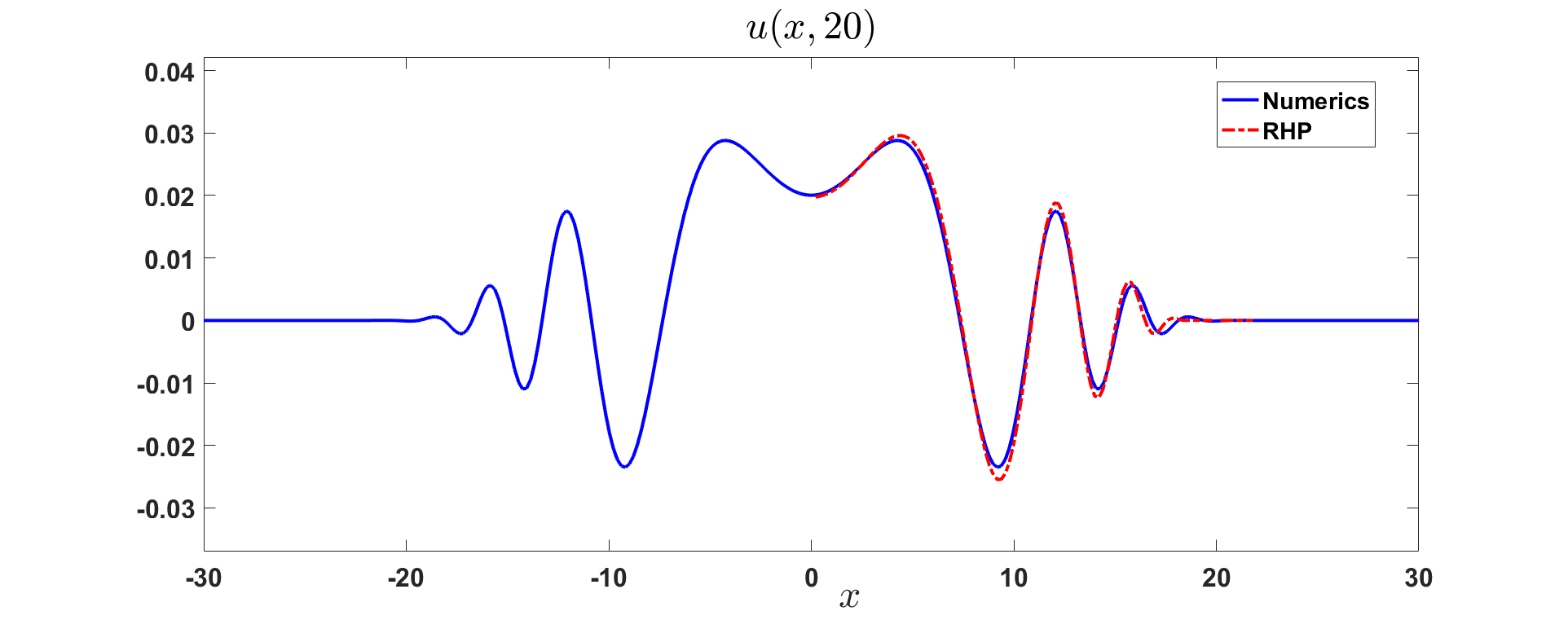
Figure 2. The comparisons of asymptotic expressions given in Theorem 2.7 and full numerical simulations of the Tzitzéica equation (1.2) with initial condition (2.4) at time $t=20$.

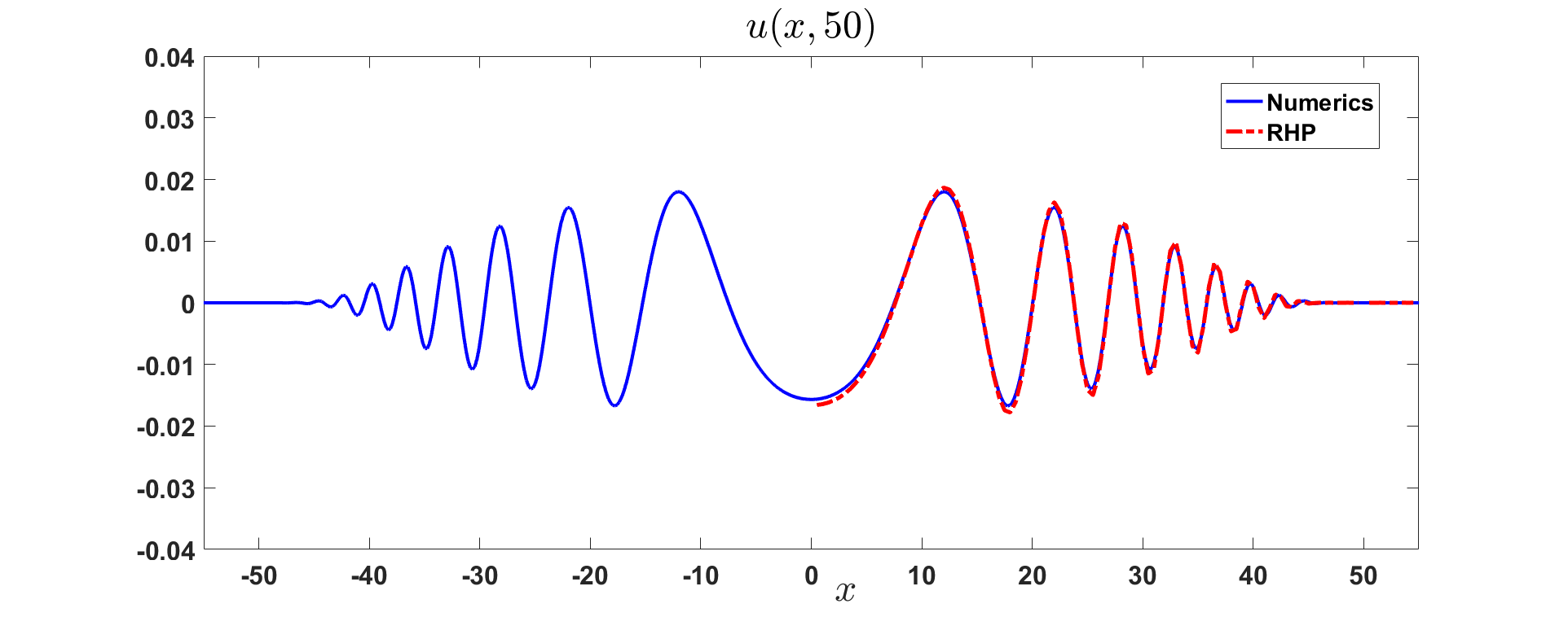
Figure 3. The comparisons of asymptotic expressions given in Theorem 2.7 and full numerical simulations of the Tzitzéica equation (1.2) with initial condition (2.4) at time $t=50$.

3. Spectral analysis

3.1. Lax pair

The Tzitzéica equation (1.2) satisfies the following Lax pair

$$\left\{\begin{array}[]{l}\phi_{x}(x,t,\lambda)=L(x,t,\lambda)\phi(x,t,\lambda),\\ \phi_{t}(x,t,\lambda)=Z(x,t,\lambda)\phi(x,t,\lambda),\end{array}\right.$$ (3.1)

and $L$ and $Z$ satisfy

$$L(x,t,\lambda)=\frac{\lambda}{2}J+U_{0}+\frac{1}{\lambda}U_{1},$$ (3.2)

$$Z(x,t,\lambda)=\frac{\lambda}{2}J+U_{0}-\frac{1}{\lambda}U_{1},$$ (3.3)

with

$$J=\left(\begin{array}[]{ccc}\omega&0&0\\ 0&\omega^{2}&0\\ 0&0&1\end{array}\right),\ U_{0}=\frac{i\sqrt{3}\left(u_{x}+u_{t}\right)}{6}\left(\begin{array}[]{ccc}0&1&-1\\ -1&0&1\\ 1&-1&0\end{array}\right),$$

$$U_{1}=\frac{1}{6}\left(\begin{array}[]{ccc}\omega^{2}\left(2e^{u}+e^{-2u}\right)&e^{-2u}-e^{u}&\omega\left(e^{-2u}-e^{u}\right)\\ e^{-2u}-e^{u}&\omega\left(2e^{u}+e^{-2u}\right)&\omega^{2}\left(e^{-2u}-e^{u}\right)\\ \omega\left(e^{-2u}-e^{u}\right)&\omega^{2}\left(e^{-2u}-e^{u}\right)&2e^{u}+e^{-2u}\end{array}\right).$$

3.2. Direct scattering problem

Let us consider the expressions for $l_{j}$ and $z_{j}$ defined as follows:

$$l_{j}=\frac{\omega^{j}\lambda+(\omega^{j}\lambda)^{-1}}{2},\quad z_{j}=\frac{\omega^{j}\lambda-(\omega^{j}\lambda)^{-1}}{2},\quad j=1,2,3,$$

and denote $\mathcal{L}=\text{diag}(l_{1},l_{2},l_{3})=\frac{1}{2}(\lambda J+\frac{J^{2}}{\lambda})$ and $\mathcal{Z}=\text{diag}(z_{1},z_{2},z_{3})=\frac{1}{2}(\lambda J-\frac{J^{2}}{\lambda})$. The matrix functions $L$ and $Z$ in (3.1) can be written as follows

$$L:=\mathcal{L}+L_{1},\quad Z:=\mathcal{Z}+Z_{1},$$

where $L_{1},Z_{1}$ are given by

$$L_{1}=U_{0}+\frac{U_{1}-\frac{1}{2}J^{2}}{\lambda},\ Z_{1}=U_{0}-\frac{U_{1}+\frac{1}{2}J^{2}}{\lambda}.$$

Since $u_{0},u_{1}\in\mathcal{S}({\mathbb{R}})$, it is straightforward to check that the matrices $L_{1}$ and $Z_{1}$ have the following asymptotic properties

$$\lim_{|x|\rightarrow\infty}L_{1}=\lim_{|x|\rightarrow\infty}Z_{1}=0.$$ (3.4)

Noticing that $u$ is a real function, it can be directly verified that the matrix-valued functions $L$ and $Z$ satisfy the $\mathbb{Z}_{3}$ symmetry

$$L(\lambda)=\mathcal{A}^{-1}L(\omega\lambda)\mathcal{A},\quad Z(\lambda)=\mathcal{A}^{-1}Z(\omega\lambda)\mathcal{A},\quad\mathcal{A}=\left(\begin{array}[]{ccc}0&1&0\\ 0&0&1\\ 1&0&0\end{array}\right),$$ (3.5)

and the $\mathbb{Z}_{2}$ symmetry

$$L(\lambda)=\mathcal{B}\overline{L(\bar{\lambda})}\mathcal{B}^{-1},\quad Z(\lambda)=\mathcal{B}\overline{Z(\bar{\lambda})}\mathcal{B}^{-1},\quad\mathcal{B}=\left(\begin{array}[]{ccc}0&1&0\\ 1&0&0\\ 0&0&1\end{array}\right).$$ (3.6)

To facilitate the analysis, we introduce the eigenfunction $\Phi$ defined by the transformation

$$\phi=\Phi e^{\mathcal{L}x+\mathcal{Z}t},$$

then the Lax pair (3.1) can be rewritten as

$$\Phi_{x}-[\mathcal{L},\Phi]=L_{1}\Phi,$$ (3.7)

$$\Phi_{t}-[\mathcal{Z},\Phi]=Z_{1}\Phi.$$ (3.8)

The solutions to the equation (3.7) can be formalized through the introduction of two $3\times 3$ matrix-valued functions which are determined by solving specific linear Volterra integral equations. Explicitly, define $\Phi_{+}(x,\lambda)$ and $\Phi_{-}(x,\lambda)$ as follows

$$\Phi_{+}(x,\lambda)=I-\int_{x}^{\infty}e^{(x-y)\widehat{\mathcal{L}(\lambda)}}\left(L_{1}(y,\lambda)\Phi_{+}(y,\lambda)\right)dy,$$ (3.9)

$$\Phi_{-}(x,\lambda)=I+\int_{-\infty}^{x}e^{(x-y)\widehat{\mathcal{L}(\lambda)}}\left(L_{1}(y,\lambda)\Phi_{-}(y,\lambda)\right)dy,$$

where $e^{\hat{\mathcal{L}}}$ is an operator that acts on a $3\times 3$ matrix $A$ by $e^{\hat{\mathcal{L}}}A=e^{\mathcal{L}}Ae^{-\mathcal{L}}$.

Furthermore, decompose the complex plane by $\Sigma$, $i.e.$,

$$\Sigma:=\{\lambda\in\mathbb{C}|Re(l_{i})=Re(l_{j}),1\leq i<j\leq 3\},$$ (3.10)

in fact, $\Sigma$ can also be rewritten as $\Sigma:=\{{\mathbb{R}},\omega{\mathbb{R}},\omega^{2}{\mathbb{R}}\}$. Notice that $\Sigma$ divides the complex plane into six open sets $\{{D}_{j}\}_{j=1}^{6}$ (see Figure 4) and suppose $S:=\{\lambda\in\mathbb{C}|0<arg(\lambda)<\frac{2\pi}{3}\}.$

\begin{overpic}[width=260.49246pt]{sigma0.pdf} \put(57.0,48.0){$\frac{2\pi}{3}$} \put(103.0,42.0){$\Sigma$} \put(75.0,55.0){${D}_{1}$} \put(48.0,70.0){${D}_{2}$} \put(23.0,55.0){${D}_{3}$} \put(23.0,25.0){${D}_{4}$} \put(48.0,15.0){${D}_{5}$} \put(75.0,25.0){${D}_{6}$} \end{overpic}

Figure 4. The contour $\Sigma$ decomposes the $\lambda$ plane into six parts.

Proposition 3.1.

Suppose the initial data $u_{0}(x),u_{1}(x)\in\mathcal{S}({\mathbb{R}})$, then the matrix-valued Jost functions $\Phi_{+}(x,\lambda)$ and $\Phi_{-}(x,\lambda)$ have the following properties:

1. $\Phi_{+}(x,\lambda)$ is well-defined in the closure of $(S,\omega^{2}S,\omega S)\setminus\{0\}$, and $\Phi_{-}(x,\lambda)$ is well-defined in the closure of $(-S,-\omega^{2}S,-\omega S)\setminus\{0\}$. Moreover, $\Phi_{+}(\cdot,\lambda)$ and $\Phi_{-}(\cdot,\lambda)$ are smooth and rapidly decay in the closure of their domains with determinant equal to 1.

2. $\Phi_{+}(x,\cdot)$ and $\Phi_{-}(x,\cdot)$ are analytic in the interior of their domains, and any order partial derivative of $\lambda$ can be continuous to the closure of their domains.

3. $\Phi_{+}(x,\lambda)$ and $\Phi_{-}(x,\lambda)$ satisfy the following symmetric:

   $$\Phi_{\pm}(x,\lambda)=\mathcal{A}^{-1}\Phi_{\pm}(x,\omega\lambda)\mathcal{A}=\mathcal{B}{\Phi_{\pm}^{*}(x,{\lambda}^{*})}\mathcal{B}^{-1},$$

   with $\lambda$ in their domains.

4. Assuming that the initial conditions $u_{0}$ and $u_{1}$ have compact support, the functions $\Phi_{+}$ and $\Phi_{-}$ are well-defined and analytic over the complex plane $\mathbb{C}\setminus\{0\}$.

Proof.

The proof of this proposition is a straightforward analysis of the Volterra integral equations in (3.9). ∎

Remark 3.2.

For a comprehensive analysis and foundational methodologies, the reader is referred to seminal works such as those by Charlier and Lenells [8], Huang and Lenells [27], and further elaborations in [39]. At first inspection, the kernel of the integral equation in (3.9) appears to possess singularities at $\lambda=0$. This situation is reminiscent of, yet distinct from, the scenario encountered in the analysis of the Boussinesq equation, where the kernel exhibits second order poles at $\lambda=0$ as detailed in [8]. Notably, in the context of the Tzitzéica equation, the ensuing section will demonstrate that the Jost solutions can be analytically continued to $\lambda=0$, thereby indicating a significant divergence in behavior when compared to the solution characteristics of Boussinesq equation.

3.2.1. The behavior of $Jost$ functions as $\lambda\to\infty$.

Next consider the behavior of the eigenfunctions $\Phi_{+}$ and $\Phi_{-}$ as $\lambda\to+\infty$. For the Lax equation (3.7) for $\Phi$, we proceed by conducting a Wentzel–Kramers–Brillouin (WKB) expansion of $\Phi$ as $\lambda\rightarrow\infty$, which yields the series

$$\Phi_{\pm}=I+\frac{\Phi^{(1)}_{\pm}}{\lambda}+\frac{\Phi^{(2)}_{\pm}}{\lambda^{2}}+\cdots,$$

where the coefficients $\Phi^{(n)}_{\pm}$ are determined by the recursive formula

$$\left\{\begin{array}[]{l}\left[\frac{J}{2},\Phi^{(n+1)}_{\pm}\right]+\left[\frac{J^{2}}{2},\Phi^{(n-1)}_{\pm}\right]=(\partial_{x}\Phi^{(n)}_{\pm})^{(o)}-\left(\mathrm{U}_{0}\Phi^{(n)}_{\pm}\right)^{(o)}-\left(\mathrm{U}_{1}\Phi^{(n-1)}_{\pm}\right)^{(o)},\\ (\partial_{x}\Phi^{(n)}_{\pm})^{(d)}=\left(\mathrm{U}_{0}\Phi^{(n)}_{\pm}\right)^{(d)}+\left(\mathrm{U}_{1}\Phi^{(n-1)}_{\pm}\right)^{(d)},\end{array}\right.$$

where $\Phi^{(0)}_{\pm}=I$ and $\Phi^{(-1)}_{\pm}=\mathbf{0}$. The notation $(\star)^{(o)}$ denotes the off-diagonal part of a matrix, whereas $(\star)^{(d)}$ refers to the diagonal part.

The following proposition describes the asymptotic properties of the Jost functions $\Phi_{+}$ and $\Phi_{-}$ when $\lambda$ tends to infinity.

Proposition 3.3.

Suppose $u_{0},u_{1}\in\mathcal{S}(\mathbb{R})$ and as $\lambda\rightarrow\infty$, the functions $\Phi_{+}$ and $\Phi_{-}$ coincide to all orders with their expansions, respectively. More precisely, let $p\geq 0$ be an integer, then the functions

$$(\Phi_{+})_{(p)}(x,\lambda):=I+\frac{\Phi^{(1)}_{+}(x)}{\lambda}+\cdots+\frac{\Phi^{(p)}_{+}(x)}{\lambda^{p}},$$

$$(\Phi_{-})_{(p)}(x,\lambda):=I+\frac{\Phi^{(1)}_{-}(x)}{\lambda}+\cdots+\frac{\Phi^{(p)}_{-}(x)}{\lambda^{p}},$$

are well-defined and, for each integer $j\geq 0$,

$$\left|\frac{\partial^{j}}{\partial\lambda^{j}}\left(\Phi_{+}-(\Phi_{+})_{(p)}\right)\right|\leq\frac{f_{+}(x)}{|\lambda|^{p+1}},\quad x\in\mathbb{R},\quad\lambda\in\left(\overline{\mathrm{S}},\omega^{2}\overline{\mathrm{S}},\omega\overline{\mathrm{S}}\right),\quad|\lambda|\geq 2,$$

$$\left|\frac{\partial^{j}}{\partial\lambda^{j}}\left(\Phi_{-}-(\Phi_{-})_{(p)}\right)\right|\leq\frac{f_{-}(x)}{|\lambda|^{p+1}},\quad x\in\mathbb{R},\quad\lambda\in\left(-\overline{\mathrm{S}},-\omega^{2}\overline{\mathrm{S}},-\omega\overline{\mathrm{S}}\right),\quad|\lambda|\geq 2,$$

where $f_{+}(x)$ and $f_{-}(x)$ are bounded smooth positive functions of $x\in\mathbb{R}$ with rapid decay as $x\rightarrow+\infty$ and $x\rightarrow-\infty$, respectively.

Proof.

This proof is similar to the case of the sine-Gordon equation and is omitted here, see [8, 27]. ∎

3.2.2. The behavior of $Jost$ functions as $\lambda\to 0$.

The presence of a pole at $\lambda=0$ in the kernel of the Jost functions signifies that the Volterra integral equation framework is not ideally suited for analyzing the behavior of Jost functions as $\lambda\to 0$. To circumvent this limitation, we propose a gauge transformation defined by $\phi(x,t;\lambda)=G(x,t)\psi(x,t;\lambda)$, where $G(x,t)$ is given by

$$G(x,t)=\frac{1+e^{u}+e^{2u}}{3e^{u}}\left(\begin{array}[]{ccc}1&\frac{\omega(e^{u}-1)}{e^{u}-\omega^{2}}&\frac{\omega^{2}(e^{u}-1)}{e^{u}-\omega}\\ \frac{\omega^{2}(e^{u}-1)}{e^{u}-\omega}&1&\frac{\omega(e^{u}-1)}{e^{u}-\omega^{2}}\\ \frac{\omega(e^{u}-1)}{e^{u}-\omega^{2}}&\frac{\omega^{2}(e^{u}-1)}{e^{u}-\omega}&1\end{array}\right).$$ (3.11)

The function $\psi(x,t;\lambda)$ satisfies a new Lax pair as following

$$\begin{cases}\psi_{x}(x,t;\lambda)=G^{-1}(LG-G_{x})\psi(x,t;\lambda)=\tilde{L}(x,t;\lambda)\psi(x,t;\lambda),\\ \psi_{t}(x,t;\lambda)=G^{-1}(ZG-G_{t})\psi(x,t;\lambda)=\tilde{Z}(x,t;\lambda)\psi(x,t;\lambda),\end{cases}$$

where

$$\tilde{L}(x,t,\lambda)=\frac{1}{2\lambda}J^{2}+\tilde{U}_{0}+\lambda\tilde{U}_{1},\ \tilde{Z}(x,t,\lambda)=\frac{1}{2\lambda}J^{2}+\tilde{U}_{0}-\lambda\tilde{U}_{1},$$

and

$$\tilde{U}_{0}=\frac{i\sqrt{3}\left(u_{x}-u_{t}\right)}{6}\left(\begin{array}[]{ccc}0&1&-1\\ -1&0&1\\ 1&-1&0\end{array}\right),$$

$$\tilde{U}_{1}=\frac{\lambda}{6}\left(\begin{array}[]{ccc}\omega\left(2e^{u}+e^{-2u}\right)&e^{-2u}-e^{u}&\omega^{2}\left(e^{-2u}-e^{u}\right)\\ e^{-2u}-e^{u}&\omega^{2}\left(2e^{u}+e^{-2u}\right)&\omega\left(e^{-2u}-e^{u}\right)\\ \omega^{2}\left(e^{-2u}-e^{u}\right)&\omega\left(e^{-2u}-e^{u}\right)&2e^{u}+e^{-2u}\end{array}\right).$$

Hence one has

$$\tilde{L}\sim\frac{1}{2}(\frac{J^{2}}{\lambda}+\lambda J),\quad\tilde{Z}\sim\frac{1}{2}(\frac{J^{2}}{\lambda}+\lambda J),\quad x\to\pm\infty,$$

and suppose that

$$\tilde{\mathcal{L}}=\frac{1}{2}(\frac{J^{2}}{\lambda}+\lambda J),\quad\tilde{\mathcal{Z}}=\frac{1}{2}(\frac{J^{2}}{\lambda}-\lambda J),$$

$$\tilde{L}_{1}:=\tilde{U}_{0}+\lambda\tilde{U}_{1},\quad\tilde{Z}_{1}:=\tilde{U}_{0}-\lambda\tilde{U}_{1}.$$

Introducing a transformation $\psi=\Psi e^{\mathcal{L}x+\mathcal{Z}t}$, we derive a new Lax pair for $\Psi$ of the form

$$\left\{\begin{array}[]{l}\Psi_{x}-[\mathcal{L},\Psi]=\tilde{L}_{1}\Psi,\\ \Psi_{t}-[\mathcal{Z},\Psi]=\tilde{Z}_{1}\Psi.\end{array}\right.$$ (3.12)

To further analyze the function $\Psi$, formulate the Volterra integral equations as follows

$$\Psi_{+}(x,\lambda)=I-\int_{x}^{\infty}e^{(x-y)\widehat{\mathcal{L}(\lambda)}}\left(\tilde{L}_{1}(y,\lambda)\Psi_{+}(y,\lambda)\right)dy,$$

$$\Psi_{-}(x,\lambda)=I+\int_{-\infty}^{x}e^{(x-y)\widehat{\mathcal{L}(\lambda)}}\left(\tilde{L}_{1}(y,\lambda)\Psi_{-}(y,\lambda)\right)dy.$$

This formulation ensures that the kernel of the Volterra integral equations is not affected by the poles as $\lambda\to 0$. Consequently, we propose a formal expansion of function $\Psi$ for $\lambda\to 0$, given by

$$\Psi_{\pm}(x,\lambda)=\Psi_{\pm}^{(0)}(x)+\Psi_{\pm}^{(1)}(x)\lambda+\cdots,\quad\text{as}\ \lambda\to 0.$$

Combining the formal expansion above with the $x$-part of Lax pair (3.12), we arrive at the following system of equations

$$\left\{\begin{array}[]{l}{\left[\frac{J}{2},\Psi^{(n-1)}_{\pm}\right]+\left[\frac{J^{2}}{2},\Psi^{(n+1)}_{\pm}\right]=(\partial_{x}\Psi^{(n)}_{\pm})^{(o)}-\left(\tilde{U}_{0}\Psi^{(n)}_{\pm}\right)^{(o)}-\left(\tilde{U}_{1}\Psi^{(n-1)}_{\pm}\right)^{(o)},}\\ (\partial_{x}\Psi^{(n)}_{\pm})^{(d)}=\left(\tilde{U}_{0}\Psi^{(n)}_{\pm}\right)^{(d)}+\left(\tilde{U}_{1}\Psi^{(n-1)}_{\pm}\right)^{(d)},\end{array}\right.$$

where $\Psi_{\pm}^{(0)}(x)=I$ and $\Psi_{\pm}^{(-1)}(x)=0$. In this context, the behavior of $\Phi(x,\lambda)$ as $\lambda\to 0$ is described through the transformation $\Phi=G\Psi$, leading to the expansion:

$$\Phi_{\pm}(x,\lambda)=G(x)+G\Psi_{\pm}^{(1)}(x)\lambda+\cdots,\quad\text{as}\ \lambda\to 0.$$

Remark 3.4.

Here are several properties of the function $G(x,t)$:

• The function $G=G(x,t)$ satisfies the symmetries

  $$\mathcal{A}^{-1}G\mathcal{A}=G,\quad\mathcal{B}G\mathcal{B}=G.$$

• Notice that

  $$\left(\begin{array}[]{lll}\omega&\omega^{2}&1\end{array}\right)G(x,t) =e^{u}\left(\begin{array}[]{lll}\omega&\omega^{2}&1\end{array}\right),$$

  $$\left(\begin{array}[]{lll}\omega&\omega^{2}&1\end{array}\right)G(x,t)^{-1} =e^{-u}\left(\begin{array}[]{lll}\omega&\omega^{2}&1\end{array}\right).$$

  Due to these properties, the reconstruction of the solution to the Tzitzéica equation as $\lambda$ approaches zero becomes a viable endeavor.

Remark 3.5.

In contrast to the scenario encountered with the Boussinesq equation, the Jost functions pertaining to the isospectral problem for the Tzitzéica equation exhibit regularity at $\lambda=0$. This distinction underscores a fundamental difference in the analytical properties of the solutions associated with these two equations, highlighting the unique behavior of the Tzitzéica equation in the context of singularities at the origin of the spectral parameter.

3.3. The scattering matrix

Suppose the initial potential functions $u_{0}$ and $u_{1}$ in (1.3) have compact support, then there exists a matrix function $s(\lambda)$ dependent of $x$ and $t$ such that the following relationship holds

$$\Phi_{+}(x,\lambda)=\Phi_{-}(x,\lambda)e^{x\widehat{\mathcal{L}(\lambda)}}s(\lambda),\quad\lambda\in\mathbb{C}\setminus\{0\},$$

which characterizes the analytic continuation of the scattering data across the complex plane, excluding the origin. In the more general case where $\{u_{0},u_{1}\}\in\mathcal{S}(\mathbb{R})$, the aforementioned relationship for $s(\lambda)$ remains valid within its domain.

Proposition 3.6.

Suppose $u_{0},u_{1}\in\mathcal{S}({\mathbb{R}})$, then the matrix function $s(\lambda)$ has the following properties:

1. The domain of function $s(\lambda)$ is

   $$\left(\begin{array}[]{ccc}\bar{S}&\mathbb{R}_{+}&\omega\mathbb{R}_{+}\\ \mathbb{R}_{+}&\omega^{2}\bar{S}&\omega^{2}\mathbb{R}_{+}\\ \omega\mathbb{R}_{+}&\omega^{2}\mathbb{R}_{+}&\omega\bar{S}\end{array}\right)\setminus\{0\},$$

   where $\overline{S}$ means the closure of set $S$, and ${\mathbb{R}}_{+}$ and ${\mathbb{R}}_{-}$ represent the positive and negative real axis respectively. The function $s(\lambda)$ is continuous to the boundary of its domain but only analytic in the interior of its domain.

2. The behaviors of $s(\lambda)$ as $\lambda\to 0$ and $\lambda\to\infty$, respectively are

   $$s(\lambda)=I-\sum_{j=1}^{N}\frac{s_{j}}{\lambda^{j}}+\mathcal{O}\left(\frac{1}{\lambda^{N+1}}\right),\quad\lambda\rightarrow\infty,$$

   and

   $$s(\lambda)=I+s^{(1)}\lambda+\cdots,\quad\lambda\rightarrow 0.$$

3. Function $s(\lambda)$ satisfies the symmetries

   $$s(\lambda)=\mathcal{A}^{-1}s(\omega\lambda)\mathcal{A}=\mathcal{B}s^{*}({\lambda}^{*})\mathcal{B}^{-1}.$$

Proof.

Let us consider the $\lambda$ lies within the intersection of the relevant domain. The relationship between the Jost functions $\Phi_{+}$ and $\Phi_{-}$ can be expressed as:

$$\Phi_{+}(x,\lambda)=\Phi_{-}(x,\lambda)e^{x\widehat{\mathcal{L}(\lambda)}}s(\lambda).$$

It is noteworthy that as $x\to-\infty$, $\Phi_{-}(x,\lambda)$ converges rapidly towards the identity matrix $I$. This observation allows us to represent $s(\lambda)$ in the following integral

$$s(\lambda)=I-\int_{-\infty}^{\infty}e^{-y\widehat{\mathcal{L}(\lambda)}}\left(L_{1}(y,\lambda)\Phi_{+}(y,\lambda)\right)dy.$$ (3.13)

Through a detailed analysis of the exponential terms $e^{l_{i}-l_{j}}$, it is directly to show that

$$\lambda\in\left(\begin{array}[]{ccc}\bar{S}&\mathbb{R}_{+}&\omega\mathbb{R}_{+}\\ \mathbb{R}_{+}&\omega^{2}\bar{S}&\omega^{2}\mathbb{R}_{+}\\ \omega\mathbb{R}_{+}&\omega^{2}\mathbb{R}_{+}&\omega\bar{S}\end{array}\right)\setminus\{0\}.$$

Furthermore, the analysis of the behavior of $\Phi(x,\lambda)$ as $\lambda\to 0$, and letting $x=0$, it shows that

$$G(0)+G(0)\Psi_{+}^{(1)}(0)\lambda+\mathcal{O}(\lambda)=(G(0)+G(0)\Psi_{-}^{(1)}(0)\lambda+\mathcal{O}(\lambda))s(\lambda)$$

which allows us to find the expansion of $s(\lambda)$ as $\lambda\to 0$. Consequently, the expansion of $s(\lambda)$ is given by

$$s(\lambda)=I+s^{(1)}\lambda+\cdots\quad\lambda\to 0,$$

where the coefficients $s^{(j)}$ are determined by the relation $s^{(j)}=\left(\Psi_{-}^{(j)}\right)^{-1}\Psi_{+}^{(j+1)}$. ∎

Remark 3.7.

In fact, by the third property of scattering matrix $s(\lambda)$, the domain of $s(\lambda)$ can be analytic continuous to the point $\lambda=0$.

3.4. The Cofactor matrix

Let $M^{A}$ denote the cofactor of matrix $M$, defined by $M^{A}=(M^{-1})^{T}$. Utilizing the space part of Lax pair presented in (3.7), we derive a corresponding Lax representation for the cofactor matrix associated with the Jost functions, given by

$$\Phi_{x}^{A}+[\mathcal{L},\Phi^{A}]=-L_{1}^{T}\Phi^{A}.$$

To express the Volterra integral equations for $\Phi^{A}$, analogous formulations to those previously discussed are employed, which yields

$$\Phi_{+}^{A}(x,\lambda)=I+\int_{x}^{\infty}e^{-(x-y)\widehat{\mathcal{L}(\lambda)}}\left(L_{1}^{T}\Phi_{+}^{A}\right)(y,\lambda)\,dy,$$

$$\Phi_{-}^{A}(x,\lambda)=I-\int_{-\infty}^{x}e^{-(x-y)\widehat{\mathcal{L}(\lambda)}}\left(L_{1}^{T}\Phi_{-}^{A}\right)(y,\lambda)\,dy.$$

The application of a similar analysis to these Volterra integral equations for $\Phi^{A}$ as conducted for $\Phi$ leads to a new proposition regarding the Jost functions, denoted $\Phi^{A}_{\pm}$.

Proposition 3.8.

Suppose the initial data $u_{0}(x),u_{1}(x)\in\mathcal{S}(x)$, then cofactor matrix of Jost functions $\Phi_{+}^{A}(x,\lambda)$ and $\Phi_{-}^{A}(x,\lambda)$ have the following properties:

1. $\Phi_{+}^{A}(x,\lambda)$ is well-defined in the closure of $(-S,-\omega^{2}S,-\omega S)\setminus\{0\}$, and $\Phi_{-}^{A}(x,\lambda)$ is well-defined in the closure of $(S,\omega^{2}S,\omega S)\setminus\{0\}$, the determinant of $\Phi^{A}_{\pm}$ are always equal to $1$, and $\Phi_{+}^{A}(\cdot,\lambda)$ and $\Phi_{-}^{A}(\cdot,\lambda)$ are smooth and rapidly decay in the closure of their domains.

2. $\Phi_{+}^{A}(x,\cdot)$ and $\Phi_{-}^{A}(x,\cdot)$ are analytic in the interior of their domains, but any order partial derivative of $k$ can be continuous to the closure of their domains.

3. $\Phi_{+}^{A}(x,\lambda)$ and $\Phi_{-}^{A}(x,\lambda)$ satisfy the following symmetries

   $$\Phi_{\pm}^{A}(x,\lambda)=\mathcal{A}^{-1}\Phi_{\pm}^{A}(x,\omega\lambda)\mathcal{A}=\mathcal{B}{(\Phi_{\pm}^{A})^{*}(x,{\lambda}^{*})}\mathcal{B}^{-1},$$

   where $\lambda$ is in the domains of $\Phi_{+}^{A}(x,\lambda)$ and $\Phi_{-}^{A}(x,\lambda)$.

4. Assuming that the initial conditions $u_{0}$ and $u_{1}$ have compact support, $\Phi_{+}^{A}$ and $\Phi_{-}^{A}$ are well-defined and analytic for $\lambda\in{\mathbb{C}}\setminus\{0\}$.

Proposition 3.9.

Suppose $u_{0},u_{1}\in\mathcal{S}(\mathbb{R})$ and as $\lambda\rightarrow\infty,\Phi_{+}^{A}$ and $\Phi_{-}^{A}$ coincide to all orders with their expansions like $(\Phi_{\pm})_{(p)}$, respectively. More precisely, let $p\geq 0$ be an integer, then the functions

$$(\Phi_{+}^{A})_{(p)}(x,\lambda):=I+\frac{(\Phi^{A}_{+})^{(1)}(x)}{\lambda}+\cdots+\frac{(\Phi^{A}_{+})^{(p)}(x)}{\lambda^{p}},$$

$$(\Phi_{-}^{A})_{(p)}(x,\lambda):=I+\frac{(\Phi^{A}_{-})^{(1)}(x)}{\lambda}+\cdots+\frac{(\Phi^{A}_{-})^{(p)}(x)}{\lambda^{p}},$$

are well-defined and, for each integer $j\geq 0$, one has

$$\left|\frac{\partial^{j}}{\partial\lambda^{j}}\left(\Phi_{+}^{A}-(\Phi_{+}^{A})_{(p)}\right)\right|\leq\frac{g_{+}(x)}{|\lambda|^{p+1}},\quad x\in\mathbb{R},\quad\lambda\in\left(-\overline{\mathrm{S}},-\omega^{2}\overline{\mathrm{S}},-\omega\overline{\mathrm{S}}\right),\quad|\lambda|\geq 2,$$

$$\left|\frac{\partial^{j}}{\partial\lambda^{j}}\left(\Phi_{-}^{A}-(\Phi_{-}^{A})_{(p)}\right)\right|\leq\frac{g_{-}(x)}{|\lambda|^{p+1}},\quad x\in\mathbb{R},\quad\lambda\in\left(\overline{\mathrm{S}},\omega^{2}\overline{\mathrm{S}},\omega\overline{\mathrm{S}}\right),\quad|\lambda|\geq 2,$$

where $g_{+}(x)$ and $g_{-}(x)$ are bounded smooth positive functions of $x\in\mathbb{R}$ with rapid decay behaviors as $x\rightarrow+\infty$ and $x\rightarrow-\infty$, respectively.

By the definition of $M^{A}$, it follows naturally that $\Phi^{A}=G^{A}\Psi^{A}$. Consequently, the function $\Psi^{A}$ is governed by the equation

$$\Psi_{x}^{A}+[\mathcal{L},\Psi^{A}]=-(G^{-1}LG-GG_{x}-\mathcal{L})\Psi^{A}=-\tilde{L}_{1}^{T}\Psi^{A}.$$

The Volterra integral equations for the cofactor matrix functions $\Psi^{A}$ are expressed by

$$\Psi_{+}^{A}(x,\lambda)=I+\int_{x}^{\infty}e^{-(x-y)\widehat{\mathcal{L}(\lambda)}}\left(\tilde{L}_{1}^{T}\Psi_{+}^{A}\right)(y,\lambda)dy,$$

$$\Psi_{-}^{A}(x,\lambda)=I-\int_{-\infty}^{x}e^{-(x-y)\widehat{\mathcal{L}(\lambda)}}\left(\tilde{L}_{1}^{T}\Psi_{-}^{A}\right)(y,\lambda)dy.$$

Analogous to the analysis for $\Psi_{\pm}$ as $\lambda\to 0$, the expansion for $\Psi^{A}_{\pm}$ near $\lambda=0$ is given by

$$\Psi_{\pm}^{A}(x,\lambda)=(\Psi_{\pm}^{A})^{(0)}(x)+(\Psi_{\pm}^{A})^{(1)}(x)\lambda+\cdots,\quad\text{as}\ \lambda\to 0,$$

where $(\Psi_{\pm}^{A})^{(0)}(x)=I$.

The analysis of the scattering matrix $s^{A}(\lambda)$ parallels that of $s(\lambda)$, with the relationship between the Jost functions $\Phi_{+}^{A}$ and $\Phi_{-}^{A}$ given by

$$\Phi_{+}^{A}(x,\lambda)=\Phi_{-}^{A}(x,\lambda)e^{-x\widehat{\mathcal{L}(\lambda)}}s^{A}(\lambda),\quad\lambda\in\mathbb{C}\setminus\{0\},$$

where the matrix-valued function $s^{A}(\lambda)$ is

$$s^{A}(\lambda)=I+\int_{-\infty}^{\infty}e^{y\widehat{\mathcal{L}(\lambda)}}\left(L_{1}^{T}(y,\lambda)\Phi_{+}^{A}(y,\lambda)\right)dy.$$ (3.14)

In the following proposition, we provide a brief overview of the relevant properties of $s^{A}(\lambda)$. The detailed derivation and proof process are omitted.

Proposition 3.10.

Let us consider the initial data $u_{0},u_{1}\in\mathcal{S}(\mathbb{R})$, then the matrix function $s^{A}(\lambda)$ exhibits the ensuing properties:

1. The domain of function $s^{A}(\lambda)$ is

   $$\left(\begin{array}[]{ccc}-\bar{S}&\mathbb{R}_{-}&\omega\mathbb{R}_{-}\\ \mathbb{R}_{-}&-\omega^{2}\bar{S}&\omega^{2}\mathbb{R}_{-}\\ \omega\mathbb{R}_{-}&\omega^{2}\mathbb{R}_{-}&-\omega\bar{S}\end{array}\right)\setminus\{0\}.$$

2. The behaviors of $s^{A}(\lambda)$ as $\lambda\to 0$ and $\lambda\to\infty$, respectively, are

   $$s^{A}(\lambda)=I-\sum_{j=1}^{N}\frac{s_{j}^{A}}{\lambda^{j}}+\mathcal{O}\left(\frac{1}{\lambda^{N+1}}\right),\quad\lambda\rightarrow\infty,$$

   and

   $$s^{A}(\lambda)=I+(s^{A})^{(1)}\lambda+\cdots,\quad\lambda\rightarrow 0.$$

3. The matrix function $s^{A}(\lambda)$ satisfies the symmetries

   $$s^{A}(\lambda)=\mathcal{A}^{-1}s^{A}(\omega\lambda)\mathcal{A}=\mathcal{B}(s^{A})^{*}({\lambda}^{*})\mathcal{B}^{-1}.$$

3.5. The eigenfunctions $M_{n}$.

In this subsection, we construct the piecewise holomorphic eigenfunctions $M_{n}$ restricted in the region $D_{n}=\{\lambda:\frac{(n-1)\pi}{3}<\arg(\lambda)<\frac{n\pi}{3}\}$ for $n=1,2,\cdots,6$.

For $\lambda\in D_{n}$, define a $3\times 3$ matrix function by Fredholm integral equation

$$\left(M_{n}\right)_{ij}(x,\lambda)=\delta_{ij}+\int_{\gamma_{ij}^{n}}\left(e^{\left(x-y\right)\widehat{\mathcal{L}(\lambda)}}\left(L_{1}M_{n}\right)\left(y,\lambda\right)\right)_{ij}dy,\quad i,j=1,2,3,$$ (3.15)

where the contours $\gamma_{ij}^{n}$ for $n=1,2,\ldots,6$ and $i,j=1,2,3$, are defined as follows

$$\gamma_{ij}^{n}=\left\{\begin{array}[]{ll}(-\infty,x),&\operatorname{Re}l_{i}(\lambda)<\operatorname{Re}l_{j}(\lambda),\\ (+\infty,x),&\operatorname{Re}l_{i}(\lambda)\geq\operatorname{Re}l_{j}(\lambda),\end{array}\quad\text{ for }\quad\lambda\in D_{n}.\right.$$

Denote the zeros of the Fredholm determinants related to the Fredholm integral equations as $\mathcal{N}$ and suppose $\tilde{\mathcal{N}}:=\mathcal{N}\cup\{0\}$. Moreover, the $3\times 3$ matrix-valued function defined by (3.15) has the following propositions.

Proposition 3.11.

Assume $u_{0},u_{1}\in\mathcal{S}({\mathbb{R}})$, then Fredholm integral equation (3.15) defines $3\times 3$ matrix valued functions $M_{n}$ that have the following properties:

1. The matrix-valued function $M_{n}(x,\lambda)$ is defined in ${\mathbb{R}}\times\bar{D}_{n}\setminus\tilde{\mathcal{N}}$ . Furthermore, $M(\cdot,\lambda)$ is a smooth function for $\lambda\in D_{n}\setminus\tilde{\mathcal{N}}$ and satisfies the Lax pair.

2. For any $x\in{\mathbb{R}}$, the matrix-valued function $M_{n}(x,\cdot)$ is holomorphic in $\lambda\in D_{n}\setminus\tilde{\mathcal{N}}$ and continuous on $\lambda\in\bar{D}_{n}\setminus\tilde{\mathcal{N}}$.

3. $\forall\epsilon>0$, $M_{n}(x,\lambda)$ is a bounded matrix function for $x\in{\mathbb{R}}$ and $\lambda\in D_{n},\text{dist}(\lambda,\tilde{\mathcal{N}})\geq\epsilon$.

4. $\det M_{n}(x,\lambda)=1$ for $x\in{\mathbb{R}}$ and $\lambda\in\bar{D}_{n}\setminus{\tilde{\mathcal{N}}}$.

5. $\forall x\in{\mathbb{R}}$, define the piecewise holomorphic matrix function $M(x,\lambda):=M_{n}(x,\lambda)$ for $\lambda\in D_{n}$ and the matrix function $M(x,\lambda)$ is suited to the following symmetries

   $$M(x,\lambda)=\mathcal{A}^{-1}M(x,\omega\lambda)\mathcal{A}=\mathcal{B}{M^{*}(x,{\lambda}^{*})}\mathcal{B}^{-1},\quad\lambda\in{\mathbb{C}}\setminus{\tilde{\mathcal{N}}}.$$

Proof.

Without loss of generality, we only focus on the first column of $M_{1}(x;\lambda)$ and introduce $m_{i}(x;\lambda)$ as the $(i,1)$ item in $M_{1}(x;\lambda)$ as

$$m(x,\lambda)_{i}=(\delta)_{i1}+\int_{{\mathbb{R}}}\sum_{j=1}^{3}K(x,y;\lambda)_{ij}m_{j}(y,\lambda)dy,$$

where

$$K\left(x,y;\lambda\right)_{ij}=\pm H(x-y)e^{(x-y)(l_{i}-l_{1})}(L_{1})_{ij},$$

the $\pm\infty$ with respect to the choice of $\gamma_{ij}$, and $|L_{1}(x)|$ could be dominated by a Schwartz function $b(x)$. Moreover, the Fredholm determinant associated to the first column is

$$f(\lambda)=\sum_{m=0}^{\infty}\frac{(-1)^{m}}{m!}\sum_{i_{1},i_{2},\ldots,i_{m}=1}^{3}\int_{\mathbb{R}^{m}}K^{(m)}\left(\begin{array}[]{l}x_{1},i_{1},x_{2},i_{2},\ldots,x_{m},i_{m}\\ x_{1},i_{1},x_{2},i_{2},\cdots,x_{m},i_{m}\end{array};\lambda\right)dx_{1}dx_{2}\cdots dx_{m}$$

with

$$K^{(m)}\left(\begin{array}[]{l}x_{1},i_{1},x_{2},i_{2},\ldots,x_{m},i_{m}\\ y_{1},i_{1}^{\prime},y_{2},i_{2}^{\prime},\cdots,y_{m},i_{m}^{\prime}\end{array};\lambda\right)=\operatorname{det}\left(\begin{array}[]{ccc}K\left(x_{1},y_{1},\lambda\right)_{i_{1}i_{1}^{\prime}}&\cdots&K\left(x_{1},y_{m},\lambda\right)_{i_{1}i_{m}^{\prime}}\\ \vdots&&\vdots\\ K\left(x_{m},y_{1},\lambda\right)_{i_{m}i_{1}^{\prime}}&\cdots&K\left(x_{m},y_{m},\lambda\right)_{i_{m}i_{m}^{\prime}}\end{array}\right).$$

Using the Hardamard’s inequality, it is immediate to know that

$$|K^{(m)}|\leq m^{m/2}\Pi_{j=1}^{m}b(y_{j}).$$

Consequently, the Fredholm determinant $f$ related to the first column of (3.15) is a holomorphic function for $\lambda\in{D}_{1}\setminus{\tilde{\mathcal{N}}}$ and continuous to the closure of ${D}_{1}\setminus{\tilde{\mathcal{N}}}$. Furthermore, since the potential matrix $\tilde{L}_{1}$ is $\mathcal{O}(1)$ as $\lambda\to\infty$, the Fredholm determinant $f$ is bounded as $\lambda\to\infty$ so that the zeros of $f$ is finite in the region $D_{1}$.

∎

Lemma 3.12.

Suppose $u_{0},u_{1}\in\mathcal{S}({\mathbb{R}})$ with compact support, then

$$M_{n}(x,\lambda) =\Phi_{-}(x,\lambda)e^{x\mathcal{L}(\lambda)}S_{n}(\lambda)e^{-x\mathcal{L}(\lambda)}$$

$$=\Phi_{+}(x,\lambda)e^{x\mathcal{L}(\lambda)}T_{n}(\lambda)e^{-x\mathcal{L}(\lambda)},\quad n=1,2,\ldots,6,$$

where the matrices $T_{n}(\lambda)$ and $S_{n}(\lambda)$ can be expressed by the elements of the matrix $s(\lambda)$ and the $(ij)$-th minor $m_{ij}(s)$ of $s(\lambda)$, which are expressed by

$$\begin{array}[]{rlr}S_{1}(\lambda)=\left(\begin{array}[]{ccc}s_{11}&0&0\\ s_{21}&\frac{m_{33}(s)}{s_{11}}&0\\ s_{31}&\frac{m_{23}(s)}{s_{11}}&\frac{1}{m_{33}(s)}\end{array}\right),&S_{2}(\lambda)=\left(\begin{array}[]{ccc}s_{11}&0&0\\ s_{21}&\frac{1}{m_{22}(s)}&\frac{m_{32}(s)}{s_{11}}\\ s_{31}&0&\frac{m_{22}(s)}{s_{11}}\end{array}\right),\\ S_{3}(\lambda)=\left(\begin{array}[]{ccc}\frac{m_{22}(s)}{s_{33}}&0&s_{13}\\ \frac{m_{12}(s)}{s_{33}}&\frac{1}{m_{22}(s)}&s_{23}\\ 0&0&s_{33}\end{array}\right),&S_{4}(\lambda)=\left(\begin{array}[]{ccc}\frac{1}{m_{11}(s)}&\frac{m_{21}(s)}{s_{33}}&s_{13}\\ 0&\frac{m_{11}(s)}{s_{33}}&s_{23}\\ 0&0&s_{33}\end{array}\right),\\ S_{5}(\lambda)=\left(\begin{array}[]{ccc}\frac{1}{m_{11}(s)}&s_{12}&-\frac{m_{31}(s)}{s_{22}}\\ 0&s_{22}&0\\ 0&s_{32}&\frac{m_{11}(s)}{s_{22}}\end{array}\right),&S_{6}(\lambda)=\left(\begin{array}[]{ccc}\frac{m_{33}(s)}{s_{22}}&s_{12}&0\\ 0&s_{22}&0\\ -\frac{m_{13}(s)}{s_{22}}&s_{32}&\frac{1}{m_{33}(s)}\end{array}\right),\end{array}$$

and

$$\begin{array}[]{lll}T_{1}(\lambda)=\left(\begin{array}[]{ccc}1&-\frac{s_{12}}{s_{11}}&\frac{m_{31}(s)}{m_{33}(s)}\\ 0&1&-\frac{m_{32}(s)}{m_{33}(s)}\\ 0&0&1\end{array}\right),&T_{2}(\lambda)=\left(\begin{array}[]{ccc}1&-\frac{m_{21}(s)}{m_{22}(s)}&-\frac{s_{13}}{s_{11}}\\ 0&1&0\\ 0&-\frac{m_{23}(s)}{m_{22}(s)}&1\end{array}\right),\\ T_{3}(\lambda)=\left(\begin{array}[]{ccc}1&-\frac{m_{21}(s)}{m_{22}(s)}&0\\ 0&1&0\\ -\frac{s_{31}}{s_{33}}&-\frac{m_{23}(s)}{m_{22}(s)}&1\end{array}\right),&T_{4}(\lambda)=\left(\begin{array}[]{ccc}1&0&0\\ -\frac{m_{12}(s)}{m_{11}(s)}&1&0\\ \frac{m_{13}(s)}{m_{11}(s)}&-\frac{s_{32}}{s_{33}}&1\end{array}\right),\\ T_{5}(\lambda)=\left(\begin{array}[]{ccc}1&0&0\\ -\frac{m_{12}(s)}{m_{11}(s)}&1&-\frac{s_{23}}{s_{22}}\\ \frac{m_{13}(s)}{m_{11}(s)}&0&1\end{array}\right),&T_{6}(\lambda)=\left(\begin{array}[]{ccc}1&0&\frac{m_{31}(s)}{m_{33}(s)}\\ -\frac{s_{21}}{s_{22}}&1&-\frac{m_{32}(s)}{m_{33}(s)}\\ 0&0&1\end{array}\right).\end{array}$$

Proof.

Notice that

$$\left\{\begin{array}[]{l}S_{n}(\lambda)=\lim_{x\rightarrow-\infty}e^{-x\widehat{\mathcal{L}(\lambda)}}M_{n}(x,\lambda),\\ T_{n}(\lambda)=\lim_{x\rightarrow\infty}e^{-x\widehat{\mathcal{L}(\lambda)}}M_{n}(x,\lambda),\end{array}\quad\lambda\in\bar{D}_{n}\backslash\tilde{\mathcal{N}},\right.$$ (3.18)

and

$$s(\lambda)T_{n}(\lambda)=S_{n}(\lambda).$$

Furthermore, it is obvious that

$$\left(S_{n}(\lambda)\right)_{ij}=0\quad\text{ if }\quad\gamma_{ij}^{n}=(-\infty,x),$$

$$\left(T_{n}(\lambda)\right)_{ij}=\delta_{ij}\quad\text{ if }\quad\gamma_{ij}^{n}=(\infty,x).$$

The equality expressed above gives rise to nine distinct algebraic equations. For illustrative purposes, we shall focus exclusively on the region denoted as $D_{1}$. This analysis involves the matrix $\gamma^{1}$, as detailed in equation (3.15) below

$$\gamma^{1}=\left(\begin{array}[]{lll}\gamma_{2}&\gamma_{1}&\gamma_{1}\\ \gamma_{2}&\gamma_{2}&\gamma_{1}\\ \gamma_{2}&\gamma_{2}&\gamma_{2}\end{array}\right),$$

where $\gamma_{1}=(-\infty,x)$ and $\gamma_{2}=(+\infty,x)$. Thus the equation (3.18) for $n=1$ shows that

$$S_{1}=\lim_{x\rightarrow-\infty}e^{-x\widehat{L(\lambda)}}M_{1}(x,\lambda)=\left(\begin{array}[]{ccc}x_{11}&0&0\\ x_{21}&x_{22}&0\\ x_{31}&x_{32}&x_{33}\end{array}\right),$$

and

$$T_{1}=\lim_{x\rightarrow\infty}e^{-x\widehat{L(\lambda)}}M_{1}(x,\lambda)=\left(\begin{array}[]{ccc}1&y_{12}&y_{13}\\ 0&1&y_{23}\\ 0&0&1\end{array}\right).$$

The proof for the remaining cases $S_{i}(\lambda),T_{i}(\lambda)$ for $i=2,3,\cdots 5$ follows a methodology analogous to that employed for the previous discussions. ∎

Lemma 3.13.

Let $u_{0},u_{1}\in\mathcal{S}(\mathbb{R})$ and denote by $\left\{s(\lambda),M_{n}(x,\lambda)\right\}$ the spectral functions and eigenfunctions associated with the $(u_{0},u_{1})$. For any $u_{0},u_{1}\in\mathcal{S}(\mathbb{R})$, there are two function sequences $u_{0}^{(i)},u_{1}^{(i)}\in C_{0}^{\infty}({\mathbb{R}})$, which converge to $u_{0},u_{1}$ uniformly, respectively. Then it follows

$$\lim_{i\rightarrow\infty}s_{i}(\lambda)=s(\lambda),\quad\lambda\in\left(\begin{array}[]{ccc}\overline{\mathrm{S}}&\mathbb{R}_{+}&\omega\mathbb{R}_{+}\\ \mathbb{R}_{+}&\omega^{2}\overline{\mathrm{S}}&\omega^{2}\mathbb{R}_{+}\\ \omega\mathbb{R}_{+}&\omega\mathbb{R}_{+}&\omega^{2}\overline{\mathrm{S}}\end{array}\right)\backslash\{0\},$$

$$\lim_{i\rightarrow\infty}\left(s^{A}\right)_{i}(\lambda)=s^{A}(\lambda),\quad\lambda\in\left(\begin{array}[]{ccc}-\overline{\mathrm{S}}&\mathbb{R}_{-}&\omega\mathbb{R}_{-}\\ \mathbb{R}_{-}&-\omega^{2}\overline{\mathrm{S}}&\omega^{2}\mathbb{R}_{-}\\ \omega\mathbb{R}_{-}&\omega^{2}\mathbb{R}_{-}&-\omega^{2}\overline{\mathrm{S}}\end{array}\right)\backslash\{0\},$$

$$\lim_{i\rightarrow\infty}\Phi_{+}^{i}(x,\lambda)=\Phi_{+}(x,\lambda),\quad x\in\mathbb{R},\lambda\in\left(\overline{\mathrm{S}},\omega^{2}\overline{\mathrm{S}},\omega\overline{\mathrm{S}}\right)\backslash\{0\},$$

$$\lim_{i\rightarrow\infty}\Phi_{-}^{i}(x,\lambda)=\Phi_{-}(x,\lambda),\quad x\in\mathbb{R},\lambda\in\left(-\overline{\mathrm{S}},-\omega^{2}\overline{\mathrm{S}},-\omega^{2}\overline{\mathrm{S}}\right)\backslash\{0\},$$

$$\lim_{i\rightarrow\infty}M_{n}^{i}(x,\lambda)=M_{n}(x,\lambda),\quad x\in\mathbb{R},k\in\bar{D}_{n}\backslash\tilde{\mathcal{N}},\quad n=1,2,\ldots,6.$$

Lemma 3.14.

The jump matrices for the matrix functions $M_{n}(x,t,\lambda)$ associated with a Riemann-Hilbert problem are given by

$$v_{1}=\left(\begin{array}[]{ccc}1&-r_{1}(\lambda)e^{-\vartheta_{21}}&0\\ r_{1}^{*}(\lambda)e^{\vartheta_{21}}&1-\left|r_{1}(\lambda)\right|^{2}&0\\ 0&0&1\end{array}\right), v_{2}=\left(\begin{array}[]{ccc}1&0&0\\ 0&1-r_{2}(\omega\lambda)r_{2}^{*}(\omega\lambda)&-r_{2}^{*}(\omega\lambda)e^{-\vartheta_{32}}\\ 0&r_{2}(\omega\lambda)e^{\vartheta_{32}}&1\end{array}\right),$$

$$v_{3}=\left(\begin{array}[]{ccc}1-r_{1}\left(\omega^{2}\lambda\right)r_{1}^{*}\left(\omega^{2}\lambda\right)&0&r_{1}^{*}\left(\omega^{2}\lambda\right)e^{-\vartheta_{31}}\\ 0&1&0\\ -r_{1}\left(\omega^{2}\lambda\right)e^{\vartheta_{31}}&0&1\end{array}\right), v_{4}=\left(\begin{array}[]{ccc}1-\left|r_{2}(\lambda)\right|^{2}&-r_{2}^{*}(\lambda)e^{-\vartheta_{21}}&0\\ r_{2}(\lambda)e^{\vartheta_{21}}&1&0\\ 0&0&1\end{array}\right)\text{, }$$

$$v_{5}=\left(\begin{array}[]{ccc}1&0&0\\ 0&1&-r_{1}(\omega\lambda)e^{-\vartheta_{32}}\\ 0&r_{1}^{*}(\omega\lambda)e^{\vartheta_{32}}&1-r_{1}(\omega\lambda)r_{1}^{*}(\omega\lambda)\end{array}\right), v_{6}=\left(\begin{array}[]{ccc}1&0&r_{2}\left(\omega^{2}\lambda\right)e^{-\vartheta_{31}}\\ 0&1&0\\ -r_{2}^{*}\left(\omega^{2}\lambda\right)e^{\vartheta_{31}}&0&1-r_{2}\left(\omega^{2}\lambda\right)r_{2}^{*}\left(\omega^{2}\lambda\right)\end{array}\right),$$

where $\vartheta_{ij}=(l_{i}-l_{j})x+(z_{i}-z_{j})t$ and $l_{j}=\frac{\omega^{j}\lambda+(\omega^{j}\lambda)^{-1}}{2},z_{j}=\frac{\omega^{j}\lambda-(\omega^{j}\lambda)^{-1}}{2}$.

Lemma 3.15.

Suppose $u_{0},u_{1}\in\mathcal{S}(\mathbb{R})$, then the functions $M_{n}$ and $M_{n}^{A}\equiv\left(M_{n}^{-1}\right)^{T}$ for $n=1,4$ can be given by the Jost functions $\Phi_{\pm}$, $\Phi_{\pm}^{A}$ and scattering matrices $s(\lambda)$, $s^{A}(\lambda)$ as follows

$$M_{1}=\small\left(\begin{array}[]{ccc}(\Phi_{+})_{11}&\frac{(\Phi_{-}^{A})_{31}(\Phi_{+}^{A})_{23}-(\Phi_{-}^{A})_{21}(\Phi_{+}^{A})_{33}}{s_{11}}&\frac{(\Phi_{-})_{13}}{s_{33}^{A}}\\ (\Phi_{+})_{21}&\frac{(\Phi_{-}^{A})_{11}(\Phi_{+}^{A})_{33}-(\Phi_{-}^{A})_{31}(\Phi_{+}^{A})_{13}}{s_{11}}&\frac{(\Phi_{-})_{23}}{s_{33}^{A}}\\ (\Phi_{+})_{31}&\frac{(\Phi_{-})_{21}^{A}(\Phi_{+})_{13}^{A}-(\Phi_{-})_{11}^{A}(\Phi_{+})_{23}^{A}}{s_{11}}&\frac{(\Phi_{-})_{33}}{s_{33}^{A}}\end{array}\right),\quad M_{1}^{A}=\small\left(\begin{array}[]{ccc}\frac{(\Phi_{-})_{11}^{A}}{s_{11}}&\frac{(\Phi_{+})_{31}(\Phi_{-})_{23}-(\Phi_{+})_{21}(\Phi_{-})_{33}}{s_{33}^{A}}&(\Phi_{+}^{A})_{13}\\ \frac{(\Phi_{-})_{21}^{A}}{s_{11}}&\frac{(\Phi_{+})_{11}(\Phi_{-})_{33}-(\Phi_{+})_{31}(\Phi_{-})_{13}}{s_{33}^{A}}&(\Phi_{+}^{A})_{23}\\ \frac{(\Phi_{-})_{31}^{A}}{s_{11}}&\frac{(\Phi_{+})_{21}(\Phi_{-})_{13}-(\Phi_{+})_{11}(\Phi_{-})_{23}}{s_{33}^{A}}&(\Phi_{+}^{A})_{33}\end{array}\right),$$

and

$$M_{4}=\small\left(\begin{array}[]{ccc}\frac{(\Phi_{-})_{11}}{s_{11}^{A}}&\frac{(\Phi_{-}^{A})_{23}(\Phi_{+}^{A})_{31}-(\Phi_{+}^{A})_{21}(\Phi_{-}^{A})_{33}}{s_{33}}&(\Phi_{+})_{13}\\ \frac{(\Phi_{-})_{21}}{s_{11}^{A}}&\frac{(\Phi_{+}^{A})_{11}(\Phi_{-}^{A})_{33}-(\Phi_{-}^{A})_{13}(\Phi_{+}^{A})_{31}}{s_{33}}&(\Phi_{+})_{23}\\ \frac{(\Phi_{-})_{31}}{s_{11}^{A}}&\frac{(\Phi_{+}^{A})_{21}(\Phi_{-}^{A})_{13}-(\Phi_{+}^{A})_{11}(\Phi_{-}^{A})_{23}}{s_{33}}&(\Phi_{+})_{33}\end{array}\right),\quad M_{4}^{A}=\small\left(\begin{array}[]{ccc}(\Phi_{+}^{A})_{11}&\frac{(\Phi_{+})_{23}(\Phi_{-})_{31}-(\Phi_{-})_{21}(\Phi_{+})_{33}}{s_{11}^{A}}&\frac{(\Phi_{-}^{A})_{13}}{s_{33}}\\ (\Phi_{+}^{A})_{21}&\frac{(\Phi_{-})_{11}(\Phi_{+})_{33}-(\Phi_{+})_{13}(\Phi_{-})_{31}}{s_{11}^{A}}&\frac{(\Phi_{-}^{A})_{23}}{s_{33}}\\ (\Phi_{+}^{A})_{31}&\frac{(\Phi_{-})_{21}(\Phi_{+})_{13}-(\Phi_{-})_{11}(\Phi_{+})_{23}}{s_{11}^{A}}&\frac{(\Phi_{-}^{A})_{33}}{s_{33}}\end{array}\right).$$

Remark 3.16.

As the assumption illustrated, the diagonal part of scattering matrix is not equal to zero and then as $\lambda\to p_{j}$ with $p_{j}\in\mathcal{N}$, the matrix-valued function satisfies that

$$(\lambda-p_{j})M(x,t;\lambda)=0,\ \text{as}\ \lambda\to p_{j}.$$

It is immediate to know that $M(x,t;\lambda)$ can be analytically continued to the zeros of Fredholm determination.

Lemma 3.17.

Suppose $u_{0},u_{1}\in\mathcal{S}({\mathbb{R}})$, then as $\lambda\to 0$, the behavior of $M(x,t;\lambda)$ has the same expansion with $\Phi_{+}$ as $\lambda\to 0$. Specially, the leading term in the expansion is $G(x)$.

Proof.

In the process of proof, we extensively employ the methodologies outlined in [33] and [27].

For convenience, denote $\mathcal{M}_{p}(x,\lambda):=G(x)+G\Psi_{+}^{(1)}(x)\lambda+\cdots+G\Psi_{+}^{(p)}(x)\lambda^{p+1}$ and then it is sufficient to show that

$$|M(x,\lambda)-\mathcal{M}_{p}(x,\lambda)|\leq C|\lambda|^{p},\quad x\in{\mathbb{R}},\ \lambda\in{\mathbb{C}}\setminus\Gamma,\ |\lambda|<\epsilon,$$

with $\epsilon<1$ small enough.

Let $D_{n}^{\epsilon}$ be $D_{n}\cap\{|\lambda|<\epsilon\}$ and then since $G$ is a matrix function in Schwartz space, then the maximal norm of $\mathcal{M}_{p}$ is less than $1$. As a result, $\mathcal{M}_{p}^{-1}(x,\lambda)$ exists and is uniformly bounded for $\lambda\in D_{n}^{\epsilon}$ and $x\in{\mathbb{R}}$.

Now, assume that $L_{(p)}:=(\partial_{x}\mathcal{M}_{p}+\mathcal{M}_{p}\mathcal{L})\mathcal{M}_{p}^{-1}$ and $\Delta=L-L_{(p)}$, then we can get the Fredholm integral equation for $\mathcal{M}_{p}^{-1}M$ as

$$(\mathcal{M}_{p}^{-1}M)_{x}=\mathcal{M}_{p}^{-1}\Delta M+[\mathcal{L},\mathcal{M}_{p}^{-1}M]$$

heuristically, in which the each entry of $\mathcal{M}_{p}^{-1}M_{n}$ satisfies the Fredholm equation

$$\left(\mathcal{M}_{p}^{-1}M_{n}\right)(x,\lambda)_{ij}=\delta_{ij}+\int_{\gamma_{ij}^{n}}\left(e^{\left(x-y\right)\hat{\mathcal{L}}}\left(M_{(p)}^{-1}\Delta M_{n}\right)\left(y,\lambda\right)\right)_{ij}dy.$$

Let $H(x)$ be a step function with $H(x)=1$ for $x>0$ and $H(x)=0$ for $x\leq 0$, and without loss of generality, we focus on the first column of $M_{1}$ and suppose $m(x,\lambda)_{i}=(M_{1})_{i1}$, then rewrite the Fredholm equation as

$$m(x,\lambda)_{i}=(\mathcal{M}_{p})_{i1}+\int_{{\mathbb{R}}}\sum_{j=1}^{3}K(x,y;\lambda)_{ij}m_{j}(y,\lambda)dy,$$

where

$$K\left(x,y;\lambda\right)_{ij}=\sum_{s=1}^{3}\mathcal{M}_{p}(x,\lambda)_{is}H_{s}\left(x,y\right)e^{\left(l_{s}-l_{1}\right)\left(x-y\right)}\left(\mathcal{M}_{p}^{-1}\Delta\right)\left(y,\lambda\right)_{sj},$$

and

$$H_{s}\left(x,y\right)=\begin{cases}H\left(x-y\right)&\text{ if }\operatorname{Re}l_{i}(\lambda)<\operatorname{Re}l_{1}(\lambda),\\ -H\left(y-x\right)&\text{ if }\operatorname{Re}l_{i}(\lambda)\geq\operatorname{Re}l_{1}(\lambda).\end{cases}$$

Furthermore, rewrite $\Delta$ as

$$\Delta=\left(L_{1}\mathcal{M}_{p}+\left[\mathcal{L},\mathcal{M}_{p}\right]-\partial_{x}\mathcal{M}_{p}\right)\mathcal{M}_{p}^{-1}.$$

Since $\mathcal{M}_{p}^{-1}$ is uniformly bounded for $\lambda\in D_{\epsilon}^{n}$, and noticing that $L_{1}$ and $G$ are Schwartz matrix-valued functions, it follwos that there is a Schwartz function $\alpha(x)$ such that

$$|\Delta(x,\lambda)|\leq C\alpha(x)|\lambda|^{p+1},\quad x\in{\mathbb{R}},\ \lambda\in D_{n}^{\epsilon},$$

and

$$\left|K\left(x,y;\lambda\right)_{ij}\right|\leq{\alpha\left(y\right)}{|\lambda|^{p+1}},\quad x,y\in\mathbb{R},\quad\lambda\in{D}_{1}^{\epsilon}.$$

Let $K^{(0)}=1$ and define

$$K^{(m)}\left(\begin{array}[]{l}x_{1},i_{1},x_{2},i_{2},\ldots,x_{m},i_{m}\\ y_{1},i_{1}^{\prime},y_{2},i_{2}^{\prime},\cdots,y_{m},i_{m}^{\prime}\end{array};\lambda\right)=\operatorname{det}\left(\begin{array}[]{ccc}K\left(x_{1},y_{1},\lambda\right)_{i_{1}i_{1}^{\prime}}&\cdots&K\left(x_{1},y_{m},\lambda\right)_{i_{1}i_{m}^{\prime}}\\ \vdots&&\vdots\\ K\left(x_{m},y_{1},\lambda\right)_{i_{m}i_{1}^{\prime}}&\cdots&K\left(x_{m},y_{m},\lambda\right)_{i_{m}i_{m}^{\prime}}\end{array}\right).$$

Using the Hardamard’s inequality,

$$|\det(A)|^{2}\leq\prod_{i}^{m}\sum_{j}^{m}|A_{ij}|^{2},$$

it is immediate to show that

$$|K^{(m)}|\leq\left(\prod_{i}^{m}\sum_{j}^{m}|K_{ij}^{m}(x_{i},y_{j},\lambda)|^{2}\right)^{\frac{1}{2}}=m^{\frac{m}{2}}\prod_{j}^{m}\alpha(y_{j})|\lambda|^{p+1}.$$

Define the Fredholm determinant and Fredholm minor as

$$f(\lambda)=\sum_{m=0}^{\infty}f^{(m)}(\lambda),\quad\lambda\in{D}_{1}^{\epsilon},$$

$$F\left(x,y,\lambda\right)_{ii^{\prime}}=\sum_{m=0}^{\infty}F^{(m)}\left(x,y,\lambda\right)_{ii^{\prime}},\quad x,y\in{\mathbb{R}},\lambda\in{D}_{1}^{\epsilon},$$

where

$$f^{(m)}(\lambda)=\frac{(-1)^{m}}{m!}\sum_{i_{1},i_{2},\ldots,i_{m}=1}^{3}\int_{\mathbb{R}^{m}}K^{(m)}\left(\begin{array}[]{l}x_{1},i_{1},x_{2},i_{2},\ldots,x_{m},i_{m}\\ x_{1},i_{1},x_{2},i_{2},\cdots,x_{m},i_{m}\end{array};\lambda\right)dx_{1}dx_{2}\cdots dx_{m},$$

and

$$F^{(m)}(x,y,\lambda)_{ii^{\prime}}=\frac{(-1)^{m}}{m!}\sum_{i_{1},i_{2},\ldots,i_{m}=1}^{3}\int_{\mathbb{R}^{m}}K^{(m+1)}\left(\begin{array}[]{l}x,i,x_{1},i_{1},x_{2},i_{2},\ldots,x_{m},i_{m}\\ y,i^{\prime},y_{1},i_{1},y_{2},i_{2},\cdots,y_{m},i_{m}\end{array};\lambda\right)dx_{1}dx_{2}\cdots dx_{m}.$$

Therefore, the estimates for $f(\lambda)$ and $F(x,y,\lambda)$ satisfy that

$$\left|f^{(m)}(\lambda)\right|\leq\frac{3^{m}m^{m/2}\|\alpha(y)\|_{L^{1}(\mathbb{R})}^{m}|\lambda|^{(p+1)m}}{m!},\quad\lambda\in{D}_{1}^{\epsilon},m\geq 0,$$

$$\left|F^{(m)}\left(x,y,\lambda\right)_{ii^{\prime}}\right|\leq\frac{3^{m}(m+1)^{(m+1)/2}\|\alpha\|_{L^{1}(\mathbb{R})}^{m}\alpha\left(y\right)|\lambda|^{(p+1)(m+1)}}{m!},\quad x,y\in\mathbb{R},\lambda\in D_{1}^{\epsilon},m\geq 0,$$

which immediately indicates that

$$|f(\lambda)-1|\leq{C}{|\lambda|^{p+1}},\quad\lambda\in{D}_{1}^{\epsilon},$$

$$\left|F\left(x,y,k\right)\right|\leq C{\alpha(y)}{|\lambda|^{p+1}},\quad x,y\in\mathbb{R},\lambda\in{D}_{1}^{\epsilon}.$$

Notice that the Fredholm determinant is not zero for $\lambda\in D_{1}^{\epsilon}$, then by the Fredholm analysis, it yields

$$m(x,\lambda)_{i}=(\mathcal{M}_{p})_{i1}+\frac{1}{f(\lambda)}\int_{{\mathbb{R}}}\sum_{j=1}^{3}F(x,y;\lambda)_{ij}(\mathcal{M}_{p})_{j1}(y,\lambda)dy,$$

and

$$|m(x,\lambda)_{i}-(\mathcal{M}_{p})_{i1}|\leq C|\lambda|^{p+1},\quad\lambda\in D_{1}^{\epsilon}.$$

∎

3.6. Proof of Theorem 2.5

Introduce the time-dependent eigenfunctions $\{M_{n}(x,t;\lambda)\}_{n=1}^{6}$ by replacing $L_{1}(x;\lambda)$ into $L_{1}(x,t;\lambda)$ in the Fredholm integral equations and denote the sectionally holomorphic function $M(x,t;\lambda)$ as $M(x,t;\lambda)=M_{n}(x,t;\lambda)$ for $\lambda\in D_{n}$. Otherwise, the behaviour of $M(x,t;\lambda)$ has the same expansion with $\Phi_{+}$ which implies that

$$u(x,t)=\lim_{\lambda\rightarrow 0}\log\left[\left(\omega,\omega^{2},1\right)M(x,t,\lambda)\right]_{13}.$$ (3.19)

Now, it suffices to show the Theorem 2.5, if the time-dependent meromorphic matrix function $M(x,t;\lambda)$ satisfies the Lax equation and jump conditions, see Lemma 3.18 and Lemma 3.19 below.

Lemma 3.18.

For $\lambda\in D_{n}$, $M_{n}(x,t;\lambda)$ is a smooth function of $(x,t)\in{\mathbb{R}}\times[0,T)$, and satisfies the Lax pair (3.7).

Proof.

Denote $\hat{M_{n}(x,t;\lambda)}:=M_{n}(x,t;\lambda)e^{\mathcal{L}x+\mathcal{Z}t}$, it follows that $\hat{M_{n}(x,t;\lambda)}$ satisfies the space part of Lax pair and according to the compatibility conditions, we have $(\partial_{t}\hat{M_{n}}-Z\hat{M_{n}})_{x}=L(\partial_{t}\hat{M_{n}}-Z\hat{M_{n}})$. Consequently, $\partial_{t}\hat{M_{n}}-Z\hat{M_{n}}$ also solves the space part of Lax pair, but the boundary condition is 0 as $x\to\pm\infty$, w.r.t. $\gamma_{ij}^{n}$. By the Fredholm theory, for $\lambda\in D_{n}\setminus\tilde{\mathcal{N}}$, the Fredholm determinant is nonzero, which implies that the integral equation only has trivial zero solution, that is $\partial_{t}\hat{M_{n}}-Z\hat{M_{n}}\equiv 0$. Furthermore, it follows from the boundedness of $M_{n}$ and the behavior of $\lambda\to 0$ that $M_{n}(x,t;\lambda)$ satisfies the Lax pair for the Tzitzéica equation (1.2). ∎

Lemma 3.19.

For $(x,t)\in{\mathbb{R}}\times[0,T)$, the time-dependent function $M(x,t;\lambda)$ is a sectionally holomorphic function for $\lambda\in{\mathbb{C}}\setminus\Sigma$, and satisfies the same jump conditions with function $M(x;\lambda)$.

Proof.

The existence and analyticity of $M_{n}(x,t;\lambda)$ can be gotten by the standard Fredholm analysis. Moreover, we have proven that $M(x,t;\lambda)$ satisfies the Lax pair, which implies that

$$M_{n+1}(x,t;\lambda)=M_{n}(x,t;\lambda)\mathrm{e}^{\widehat{\mathcal{L}(\lambda)}x+\widehat{\mathcal{Z}(\lambda)}t}\left(M_{n}(0,0;\lambda)^{-1}M_{n+1}(0,0;\lambda)\right),$$

for $n=1,2,\cdots,6$ and $M_{7}=M_{1}$. ∎

4. Long-time asymptotics for the Tzitzéica equation

At first, focus on the critical points of RH problem 2.4 and recall the dispersive relationship $\vartheta_{21},\vartheta_{31}$ and $\vartheta_{32}$ shown in the RH problem

$$\vartheta_{21} =(l_{2}-l_{1})x+(z_{2}-z_{1})t=\frac{(\omega^{2}-\omega)t}{2}[(\lambda-\lambda^{-1})\xi+(\lambda+\lambda^{-1})],$$

where $\xi=\frac{x}{t}$, and the critical point of phase function $\vartheta_{21}$ is

$$\lambda_{0}=\pm\sqrt{\frac{|x-t|}{|x+t|}}.$$ (4.1)

Moreover, the critical point of $\vartheta_{31}$ is $\omega\lambda_{0}=\pm\omega\sqrt{\frac{|x-t|}{|x+t|}}$, while the critical point of $\vartheta_{32}$ is $\omega^{2}\lambda_{0}=\pm\omega^{2}\sqrt{\frac{|x-t|}{|x+t|}}$.

By convention, denote $B(a,\lambda_{0})=B_{\lambda_{0}}(a):=\{\lambda\in\mathbb{C}\,|\,|\lambda-a|<\lambda_{0}\}$, which represents an open disk in the complex plane centered at $a$ with radius $\lambda_{0}$, and $\partial B(a,\lambda_{0})=\partial B_{\lambda_{0}}(a):=\{\lambda\in{\mathbb{C}}||\lambda-a|=\lambda_{0}\}$, which is the boundary of $B_{\lambda_{0}}(a)$. Moreover, the signature of the real part of phase function $\vartheta_{21}$ is as follows:

1. For $|\xi|<1$, $\Re\vartheta_{21}>0$ when $\lambda\in B_{\lambda_{0}}(0)\cap\Im\lambda<0$ and $\lambda\in B^{c}_{\lambda_{0}}(0)\cap\Im\lambda>0$, while $\Re\vartheta_{21}<0$ elsewhere.

2. For $\xi\geq 1$, $\Re\vartheta_{21}>0$ when $\Im\lambda>0$, and $\Re\vartheta_{21}<0$ when $\Im\lambda<0$.

3. For $\xi\leq-1$, $\Re\vartheta_{21}>0$ when $\Im\lambda<0$, and $\Re\vartheta_{21}<0$ when $\Im\lambda>0$.

Figure 5 describes the signature of real part of phase function $\vartheta_{21}$ for $|\xi|<1$.

\begin{overpic}[width=307.85014pt]{sign.pdf} \end{overpic}

Figure 5. The signature of real part of $\vartheta_{21}$ for $|\xi|<1$: the shaded region represents $\Re\vartheta_{21}<0$ and the white region represents $\Re\vartheta_{21}>0$.

4.1. Long-time behavior outside the light cone $|\frac{x}{t}|>1$.

For $\xi>1$, we have that

$$v_{1}=\left(\begin{array}[]{ccc}1&0&0\\ r_{1}^{*}(\lambda)e^{\vartheta_{21}}&1&0\\ 0&0&1\end{array}\right)\left(\begin{array}[]{ccc}1&-r_{1}(\lambda)e^{-\vartheta_{21}}&0\\ 0&1&0\\ 0&0&1\end{array}\right):=v^{lower}_{1}v^{upper}_{1},$$

and

$$v_{4}=\left(\begin{array}[]{ccc}1&-r_{2}^{*}(\lambda)e^{-\vartheta_{21}}&0\\ 0&1&0\\ 0&0&1\end{array}\right)\left(\begin{array}[]{ccc}1&0&0\\ r_{2}(\lambda)e^{\vartheta_{21}}&1&0\\ 0&0&1\end{array}\right):=v^{upper}_{4}v^{lower}_{4}.$$

Without loss of generality, suppose that the reflection coefficient $r_{1}(\lambda)$ is analytic in the first quarter and continuous the boundary and $r_{2}(\lambda)$ is analytic in the third quarter and continuous to the boundary. Under this assumption, it is clear that $\|r_{1}(\lambda)e^{-\vartheta_{21}}\|_{\infty}$ is exponentially decay as $t\to\infty$ for $\Im\lambda>0$ which implies that the jump matrix decays to $I$ as $t\to\infty$. It follows that the solution of the RH problem 2.4 is $I$ and combining the recovering formula, we have $u(x,t)\to 0$ as $t\to\infty$. Other matrices can be factorized in the same way by using the properties of symmetric.

Lemma 4.1.

For $\xi>1$, as $t\to\infty$, the solution of RH problem 2.4 satisfies $\|M(x,t;\lambda)-I\|\to 0,\$ rapidly, and the solution of Tzitzéica equation (1.2) rapidly decays to $0$.

Proof.

Rewrite $\vartheta_{21}=\frac{-\sqrt{3}it}{2}[(\lambda-\lambda^{-1})\xi+(\lambda+\lambda^{-1})]:=2it\theta_{21}(\lambda).$ Since for $\lambda\neq 0$, $\theta_{21}$ is a monotone function of $\lambda$, we can view $\lambda$ as the function of $\theta_{21}$, and then suppose that $g(\lambda)=r_{1}(\lambda)(\lambda^{2}-i)^{2}$. Thus, it follows

$$r_{1}(\lambda)e^{-\vartheta_{21}(\lambda)} =\frac{e^{-2it\theta_{21}}}{(\lambda^{2}-i)^{2}}\frac{1}{\sqrt{2\pi}}\int_{{\mathbb{R}}}\hat{g}(s)e^{is\theta_{21}}ds=\frac{e^{-2it\theta_{21}}}{(\lambda^{2}-i)^{2}}\frac{1}{\sqrt{2\pi}}\left(\int_{-\infty}^{t}\hat{g}(s)e^{is\theta_{21}}ds+\int^{\infty}_{t}\hat{g}(s)e^{is\theta_{21}}ds\right)$$

$$:=r_{1,a}e^{-\vartheta_{21}(\lambda)}+r_{1,r}e^{-\vartheta_{21}(\lambda)},$$

where we have used the fact that

$$\hat{g}(s)=\frac{1}{\sqrt{2\pi}}\int_{{\mathbb{R}}}g(\lambda(\theta))e^{-is\theta_{21}}d\theta.$$

It is clear that $r_{1,a}e^{-\vartheta_{21}(\lambda)}$ has an analytic continuation to the upper half plane and by using the Schwartz reflection principle, the $r_{1,a}^{*}e^{\vartheta_{21}}$ is analytic in the lower half plane. Furthermore, $r_{1,a}e^{-\vartheta_{21}(\lambda)}$ decays exponentially as $t\to\infty$ in the $L^{1}\cap L^{\infty}$ norm. On the other hand, $r_{1,r}e^{-\vartheta_{21}(\lambda)}$ still relies on the positive half real line, but decays rapidly as $t\to\infty$.

In the same way, one can split $r_{2}(\lambda)e^{\vartheta_{21}}$ into $r_{2,a}(\lambda)e^{\vartheta_{21}}$ and $r_{2,r}(\lambda)e^{\vartheta_{21}}$, where $r_{2,r}(\lambda)e^{\vartheta_{21}}$ relies on the negative half line, rapidly decays as $t\to\infty$ and $r_{2,a}(\lambda)e^{\vartheta_{21}}$ can be analytic continuation to the lower plane with exponentially decaying as $t\to\infty$.

As a result, the jump matrices of RH problem 2.4 can be factorized into

$$V(x,t;\lambda)=\begin{cases}\begin{aligned} &\left(\begin{matrix}1&-r_{1,r}(\lambda)e^{-\vartheta_{21}}&0\\ r_{1,r}^{*}(\lambda)e^{\vartheta_{21}}&1-r_{1,r}(\lambda)r_{1,r}^{*}(\lambda)&0\\ 0&0&1\end{matrix}\right),&&\lambda\in\Sigma_{1}^{\prime},\\ &\left(\begin{array}[]{ccc}1&0&0\\ r_{1,a}^{*}(\lambda)e^{\vartheta_{21}}&1&0\\ 0&0&1\end{array}\right),&&\lambda\in\Sigma_{1,lower}^{\prime},\\ &\left(\begin{array}[]{ccc}1&r_{1,a}(\lambda)e^{-\vartheta_{21}}&0\\ 0&1&0\\ 0&0&1\end{array}\right),&&\lambda\in\Sigma_{1,upper}^{\prime},\\ &\left(\begin{array}[]{ccc}1-r_{2,r}(\lambda)r_{2,r}^{*}(\lambda)&-r_{2,r}^{*}(\lambda)e^{-\vartheta_{21}}&0\\ r_{2,r}(\lambda)e^{\vartheta_{21}}&1&0\\ 0&0&1\end{array}\right),&&\lambda\in\Sigma_{4}^{\prime},\\ &\left(\begin{array}[]{ccc}1&-r_{2,a}^{*}(\lambda)e^{-\vartheta_{21}}&0\\ 0&1&0\\ 0&0&1\end{array}\right),&&\lambda\in\Sigma_{4,upper},\\ &\left(\begin{array}[]{ccc}1&0&0\\ -r_{2,a}(\lambda)e^{\vartheta_{21}}&1&0\\ 0&0&1\end{array}\right),&&\lambda\in\Sigma_{4,lower},\\ \end{aligned}\end{cases}$$

and at the same time the other jump matrices can be gotten by the symmetries.

For function $f(\xi)$, define the Cauchy operator $\mathcal{C}$ on $\Sigma$ as

$$(\mathcal{C}f)(z)=\frac{1}{2\pi i}\int_{\Sigma}\frac{f(\xi)}{\xi-z}d\xi.$$

Denote $\dot{L}^{3}(\Sigma)$ as $(1+|\xi|)^{\frac{1}{3}}f(\xi)\in L^{3}(\Sigma)$, i.e., the weighted $L^{3}$ space, and Cauchy operator maps the function in $\dot{L}^{3}(\Sigma)$ into an analytic function except for $\lambda\in\Sigma$, while the boundary valued functions $\mathcal{C}_{\pm}f(z)$ belong to $\dot{L}^{3}(\Sigma)$. Suppose that $w\in L^{\infty}$, and define $\mathcal{C}_{w}$ as $\mathcal{C}_{w}(f):=\mathcal{C}_{-}(wf)$, it follows that $\mathcal{C}_{w}$ is a bounded linear operator on $\dot{L}^{3}(\Sigma)$. Let $\mu$ satisfy the following singular integral equation

$$\mu=I+\mathcal{C}_{w}\mu,\ \mu\in I+\dot{L}^{3}(\Sigma).$$

Consequently, if $(I-\mathcal{C}_{w})$ is invertible, there exits a unique solution for a RH problem with jump contour $\Sigma$ and the jump condition is $I+w$. Furthermore, the solution of this RH problem is

$$M(x,t;\lambda)=I+C(\mu w).$$

Suppose $w(x,t;\lambda)=V(x,t;\lambda)-I$, it is immediate to know that $w(x,t;\lambda)\in\dot{L}^{3}(\Sigma^{\prime})$ and $\|w(x,t;\lambda)\|_{\infty}\to 0$ rapidly as $t\to\infty$, which implies that $(I-\mathcal{C}_{w})$ is invertible. Reminding that the solution of RH problem 2.4 exists and is unique, moreover, $M_{\pm}\to I$ rapidly in $\dot{L}^{3}(\Sigma)$ norm as $t\to\infty$, thus it is concluded that $M\to I$ and $u(x,t)\to 0$ as $t\to\infty$ by the reconstruction formula $u(x,t)=\lim_{\lambda\to 0}\log\left[(\omega,\omega^{2},1)M(x,t,\lambda)\right]_{13}$. ∎

For $\xi<-1$, the signature of $\vartheta_{21}$ is opposite to the case $\xi>1$ and the factorizations of jump matrices are

$$v_{1} =\left(\begin{array}[]{ccc}1&-\frac{r_{1}(\lambda)e^{-\vartheta_{21}}}{1-|r_{1}(\lambda)|^{2}}&0\\ 0&1&0\\ 0&0&1\end{array}\right)\left(\begin{array}[]{ccc}(1-\left|r_{1}(\lambda)\right|^{2})^{-1}&0&0\\ 0&1-\left|r_{1}(\lambda)\right|^{2}&0\\ 0&0&1\end{array}\right)\left(\begin{array}[]{ccc}1&0&0\\ \frac{r_{1}^{*}(\lambda)e^{\vartheta_{21}}}{1-|r_{1}(\lambda)|^{2}}&1&0\\ 0&0&1\end{array}\right),$$

and

$$v_{4} =\left(\begin{array}[]{ccc}1&0&0\\ \frac{r_{2}^{*}(\lambda)}{1-\left|r_{2}(\lambda)\right|^{2}}e^{\vartheta_{21}}&1&0\\ 0&0&1\end{array}\right)\left(\begin{array}[]{ccc}1-\left|r_{2}(\lambda)\right|^{2}&0&0\\ 0&\frac{1}{1-\left|r_{2}(\lambda)\right|^{2}}&0\\ 0&0&1\end{array}\right)\left(\begin{array}[]{ccc}1&-\frac{r_{2}(\lambda)}{1-\left|r_{2}(\lambda)\right|^{2}}e^{-\vartheta_{21}}&0\\ 0&1&0\\ 0&0&1\end{array}\right).$$

In this case, it is necessary to introduce the functions $\delta_{1}$ and $\delta_{4}$ of the forms

$$\left\{\begin{aligned} \delta_{1+}(\lambda)&=\delta_{1-}(\lambda)\left(1-|r_{1}(\lambda)|^{2}\right),&&\lambda\in{\mathbb{R}}_{+},\\ &=\delta_{1-}(z),&&\lambda\in{\mathbb{C}}\setminus{\mathbb{R}}_{+},\\ \delta_{1}(\lambda)&\rightarrow 1&&\text{ as }\lambda\rightarrow\infty,\end{aligned}\right.$$

and

$$\left\{\begin{aligned} \delta_{4+}(\lambda)&=\delta_{4-}(\lambda)\left(1-|r_{2}(\lambda)|^{2}\right),&&k\in{\mathbb{R}}_{-},\\ &=\delta_{4-}(z),&&k\in{\mathbb{C}}\setminus{\mathbb{R}}_{-},\\ \delta_{4}(\lambda)&\rightarrow 1&&\text{ as }k\rightarrow\infty.\end{aligned}\right.$$

Thus, it follows that

$$\delta_{1}(\lambda)=\exp\left\{\frac{1}{2\pi i}\int_{0}^{\infty}\frac{\ln\left(1-\left|r_{1}(s)\right|^{2}\right)}{s-\lambda}ds\right\},\quad\lambda\in\mathbb{C}\backslash{\mathbb{R}}_{+},$$

and

$$\delta_{4}(\lambda)=\exp\left\{\frac{1}{2\pi i}\int^{-\infty}_{0}\frac{\ln\left(1-\left|r_{2}(s)\right|^{2}\right)}{s-\lambda}ds\right\},\quad\lambda\in\mathbb{C}\backslash{\mathbb{R}}_{-},$$

where we have denoted $\ln(z)$ as the real-valued function.

Using the symmetries of functions $\delta_{1}$ and $\delta_{4}$ to define $\delta_{j}$ for $j=2,3,5,6$ as follows

$$\begin{array}[]{ll}\delta_{3}(\lambda)=\delta_{1}\left(\omega^{2}\lambda\right),&\lambda\in\mathbb{C}\backslash\omega{\mathbb{R}}_{+},\\ \delta_{5}(\lambda)=\delta_{1}(\omega\lambda),&\lambda\in\mathbb{C}\backslash\omega{\mathbb{R}}_{-},\\ \delta_{2}(\lambda)=\delta_{4}\left(\omega^{2}\lambda\right),&\lambda\in\mathbb{C}\backslash\omega^{2}{\mathbb{R}}_{-},\\ \delta_{6}(\lambda)=\delta_{4}(\omega\lambda),&\lambda\in\mathbb{C}\backslash\omega^{2}{\mathbb{R}}_{+}.\end{array}$$

Define the matrix-valued function $\Delta$ as

$$\Delta(\lambda)=\left(\begin{array}[]{ccc}\frac{\delta_{1}(\lambda)\delta_{6}(\lambda)}{\delta_{3}(\lambda)\delta_{4}(\lambda)}&0&0\\ 0&\frac{\delta_{5}(\lambda)\delta_{4}(\lambda)}{\delta_{1}(\lambda)\delta_{2}(\lambda)}&0\\ 0&0&\frac{\delta_{3}(\lambda)\delta_{2}(\lambda)}{\delta_{5}(\lambda)\delta_{6}(\lambda)}\end{array}\right)=\left(\begin{array}[]{ccc}\Delta_{1}(\lambda)&0&0\\ 0&\Delta_{2}(\lambda)&0\\ 0&0&\Delta_{3}(\lambda)\end{array}\right),$$

and take the transformation

$$\tilde{M}(x,t;\lambda)=M(x,t;\lambda)\Delta(\lambda).$$

It is clear that

$$\tilde{v}_{1} =\left(\begin{array}[]{ccc}1-|r_{1}(\lambda)|^{2}&-\frac{\tilde{\delta}_{v_{1}}}{\delta_{1-}^{2}}\frac{r_{1}(\lambda)}{1-|r_{1}(\lambda)|^{2}}e^{-\vartheta_{21}}&0\\ \frac{\delta_{1+}^{2}}{\tilde{\delta}_{v_{1}}}\frac{r_{1}^{*}(\lambda)}{1-|r_{1}(\lambda)|^{2}}e^{\vartheta_{21}}&1&0\\ 0&0&1\end{array}\right)$$

$$=\left(\begin{array}[]{ccc}1&-\frac{\tilde{\delta}_{v_{1}}}{\delta_{1-}^{2}}\frac{r_{1}(\lambda)}{1-|r_{1}(\lambda)|^{2}}e^{-\vartheta_{21}}&0\\ 0&1&0\\ 0&0&1\end{array}\right)\left(\begin{array}[]{ccc}1&0&0\\ \frac{\delta_{1+}^{2}}{\tilde{\delta}_{v_{1}}}\frac{r_{1}^{*}(\lambda)}{1-|r_{1}(\lambda)|^{2}}e^{\vartheta_{21}}&1&0\\ 0&0&1\end{array}\right):=\tilde{v}_{1}^{lower}\tilde{v}_{1}^{upper},$$

and

$$\tilde{v}_{4}^{(1)} =\left(\begin{array}[]{ccc}1&-\frac{\delta_{4+}^{2}}{\tilde{\delta}_{v_{4}}}\frac{r_{2}^{*}(\lambda)}{1-|r_{2}(\lambda)|^{2}}e^{-\vartheta_{21}}&0\\ \frac{\tilde{\delta}_{v_{4}}}{\delta_{4-}^{2}}\frac{r_{2}(\lambda)}{1-|r_{2}(\lambda)|^{2}}e^{\vartheta_{21}}&1-\left|r_{2}(\lambda)\right|^{2}&0\\ 0&0&1\end{array}\right)$$

$$=\left(\begin{array}[]{ccc}1&0&0\\ \frac{\tilde{\delta}_{v_{4}}}{\delta_{4-}^{2}}\frac{r_{2}(\lambda)}{1-|r_{2}(\lambda)|^{2}}e^{\vartheta_{21}}&1&0\\ 0&0&1\end{array}\right)\left(\begin{array}[]{ccc}1&-\frac{\delta_{4+}^{2}}{\tilde{\delta}_{v_{4}}}\frac{r_{2}^{*}(\lambda)}{1-|r_{2}(\lambda)|^{2}}e^{-\vartheta_{21}}&0\\ 0&1&0\\ 0&0&1\end{array}\right):=\tilde{v}_{4}^{upper}\tilde{v}_{4}^{lower},$$

where $\tilde{\delta}_{v_{1}}=\frac{\delta_{3}\delta^{2}_{4}\delta_{5}}{\delta_{6}\delta_{2}}$ and $\tilde{\delta}_{v_{4}}=\frac{\delta_{1}^{2}\delta_{2}\delta_{6}}{\delta_{5}\delta_{3}}$.

As in the analysis for $\xi>1$, the solution of the RH problem for $\tilde{M}$ behaves $\tilde{M}\to I$ rapidly, and note that as $\lambda\to 0$, we have $r_{1}(\lambda),r_{2}(\lambda)\to 0$, which implies that the delta functions $\delta_{1}$ and $\delta_{4}$ are continuous at $\lambda=0$. By using the symmetric properties, it follows that $\delta_{1}(0)=\delta_{3}(0)=\delta_{5}(0)$ and $\delta_{4}(0)=\delta_{6}(0)=\delta_{2}(0)$. It is clear that $\Delta\to I$ as $\lambda\to 0$, and furthermore, $u(x,t)\to 0$ as $t\to\infty$ for $\xi<-1$. So the following lemma holds immediately.

Lemma 4.2.

For $\xi<-1$, as $t\to\infty$, the solution of RH problem 2.4 satisfies

$$\|M(x,t;\lambda)-I\|\to 0,\ \text{rapidly},$$

and the solution of the Tzitzéica equation (1.2) decays to zero rapidly.

4.2. Proof of the Sector I&II in Theorem 2.7

Building upon the Lemma 4.1 and Lemma 4.2, under the condition $\left|\frac{x}{t}\right|>1$ and as $t\to\infty$, the function $M(x,t,\lambda)$ converges to the identity matrix $I+\mathcal{O}(e^{-ct})$ for some positive constant $c$. While for $\left|\frac{x}{t}\right|$ tends to $\infty$, the phase function $\vartheta_{21}$ in the jump matrix is dominated by $-c|x|$, therefore, the function $M(x,t,\lambda)$ behaves like $I+\mathcal{O}(e^{-cx})$. Moreover, leveraging the explicit expression for the solution to the Tzitzéica equation (1.2), as articulated in (2.2), the result in the Sector I & II of Theorem 2.7 is proved.

4.3. Long-time behavior inside the light cone $|\frac{x}{t}|<1$.

In this subsection, the long-time asymptotics of Tzitzéica equation (1.2) inside the light cone $|\frac{x}{t}|<1$ is formulated by deforming RH problem 2.4 step by step.

4.3.1. First transformation

Recall the signature of $\vartheta_{21}$ for $|\xi|<1$, and if $|\lambda|>|\lambda_{0}|$, for $\lambda\in{\mathbb{R}}$ the jump matrix has the same factorization as in the case of $\xi>1$. On the other hand, if $\lambda$ lies inside of the circle in Figure 5, the factorization is the same as in the case of $\xi<-1$. Similarly, introduce the scalar RH problem to cancel the diagonal matrix inside the circle, abusing the same symbol for the convenience. Find functions $\delta_{1}$ and $\delta_{4}$ satisfy

$$\left\{\begin{aligned} \delta_{1+}(\lambda)&=\delta_{1-}(\lambda)\left(1-|r_{1}(\lambda)|^{2}\right),&&0<\lambda<\lambda_{0},\\ &=\delta_{1-}(z),&&\text{elsewhere},\\ \delta_{1}(\lambda)&\rightarrow 1&&\text{ as }\lambda\rightarrow\infty,\end{aligned}\right.$$

and

$$\left\{\begin{aligned} \delta_{4+}(\lambda)&=\delta_{4-}(\lambda)\left(1-|r_{2}(\lambda)|^{2}\right),&&-\lambda_{0}<\lambda<0,\\ &=\delta_{4-}(z),&&\text{elsewhere},\\ \delta_{4}(\lambda)&\rightarrow 1&&\text{ as }\lambda\rightarrow\infty.\end{aligned}\right.$$

It is immediate to see that

$$\delta_{1}(\lambda)=\exp\left\{\frac{1}{2\pi i}\int_{0}^{\lambda_{0}}\frac{\ln\left(1-\left|r_{1}(s)\right|^{2}\right)}{s-\lambda}ds\right\},\quad\lambda\in\mathbb{C}\backslash(0,\lambda_{0}),$$

and

$$\delta_{4}(\lambda)=\exp\left\{\frac{1}{2\pi i}\int^{-\lambda_{0}}_{0}\frac{\ln\left(1-\left|r_{2}(s)\right|^{2}\right)}{s-\lambda}ds\right\},\quad\lambda\in\mathbb{C}\backslash(-\lambda_{0},0).$$

Suppose that $\log_{\theta}(z)$ denotes the logarithm of $z$ with the branch cut along $\arg z=\theta$, in detail, for $\theta=0$, that is

$$\log_{0}(z)=\ln|z|+arg_{0}(z),\ arg_{0}(z)\in(0,2\pi).$$

Proposition 4.3.

The functions $\delta_{1}(\lambda)$ and $\delta_{4}(\lambda)$ are piecewise analytic for $\lambda\in(0,\lambda_{0})$ and $(-\lambda_{0},0)$, respectively, and have the properties as below:

1. The function $\delta_{1}(\lambda)$ can be rewritten as

   $$\delta_{1}(\lambda)=e^{i\nu_{1}\log_{-\pi}\left(\lambda-\lambda_{0}\right)}e^{-\chi_{1}(\lambda)},$$

   where

   $$\nu_{1}=-\frac{1}{2\pi}\ln\left(1-\left|r_{1}\left(\lambda_{0}\right)\right|^{2}\right),$$ (4.2)

   and

   $$\chi_{1}(\lambda)=\frac{1}{2\pi i}\int_{0}^{\lambda_{0}}\log_{-\pi}(\lambda-s)d\ln\left(1-\left|r_{1}(s)\right|^{2}\right).$$

   Besides, the function $\delta_{4}(\lambda)$ can be rewritten as

   $$\delta_{4}(\lambda)=e^{i\nu_{4}\log_{0}\left(\lambda+\lambda_{0}\right)}e^{-\chi_{4}(\lambda)},$$

   where

   $$\nu_{4}=-\frac{1}{2\pi}\ln\left(1-\left|r_{2}\left(-\lambda_{0}\right)\right|^{2}\right),$$ (4.3)

   and

   $$\chi_{4}(\lambda)=\frac{1}{2\pi i}\int_{0}^{-\lambda_{0}}\log_{0}(\lambda-s)d\ln\left(1-\left|r_{2}(s)\right|^{2}\right).$$

2. The functions $\delta_{1}(\lambda)$ and $\delta_{4}(\lambda)$ are piecewise analytic expect for $\lambda\in(0,\lambda_{0})$ and $(-\lambda_{0},0)$, with continuous boundary values on $[0,\lambda_{0})$ and $(-\lambda_{0},0]$, respectively.

3. The functions $\delta_{1}(\lambda)$ and $\delta_{4}(\lambda)$ satisfy the conjugate symmetry and are bounded in $|\lambda|<\lambda_{0}$, in addition, the properties below hold

   $$\delta_{1}(\lambda)={(\overline{\delta_{1}(\bar{\lambda})})^{-1}},\ k\in\mathbb{C}\backslash(0,\lambda_{0}),\quad\delta_{4}(\lambda)={(\overline{\delta_{4}(\bar{\lambda})})^{-1}},\ k\in\mathbb{C}\backslash(-\lambda_{0},0),$$

   and

   $$|\delta_{1\pm}(\lambda)|<\infty,\quad 0<\lambda<\lambda_{0},\quad|\delta_{4\pm}(\lambda)|<\infty,\quad-\lambda_{0}<\lambda<0.$$

   Moreover, $|\delta_{j}(\lambda)|$ and $|\delta_{j}^{-1}(\lambda)|~{}(j=1,4)$ are bounded.

4. As $\lambda\to\pm\lambda_{0}$ along with paths which are not tangential to $\lambda<\lambda_{0}$ and $\lambda>-\lambda_{0}$, respectively, we have

   $$\left|\chi_{1}(\lambda)-\chi_{1}\left(\lambda_{0}\right)\right|\leq C\left|\lambda-\lambda_{0}\right|\left(1+|\ln|\lambda-\lambda_{0}||\right),$$

   $$\left|\chi_{4}(\lambda)-\chi_{4}\left(-\lambda_{0}\right)\right|\leq C\left|\lambda+\lambda_{0}\right|\left(1+|\ln|\lambda+\lambda_{0}||\right).$$

Proof.

The proof of (1), (3) and (4) is standard analysis. For the (2), we claim that both $\delta_{1}$ and $\delta_{4}$ are continuous at $\lambda=0$. First of all, notice that $r_{j}(0)=0$ for $j=1,2$, so that the jump condition is continuous at $\lambda=0$. Then substituting $\lambda=0$ into the $\delta_{1}(\lambda)$, it yields

$$\delta_{1}(0)=\exp\left\{\frac{1}{2\pi i}\int_{0}^{\lambda_{0}}\frac{\ln\left(1-\left|r_{1}(s)\right|^{2}\right)}{s}ds\right\}.$$

By $\frac{\ln(1-|r_{1}(s)|^{2})}{s}=-\frac{|r_{1}(s)|^{2}}{s}$ and $|r_{1}(s)|$ decays rapidly as $s\to 0$, it is concluded that $\delta_{1}(0)$ is bounded, which implies that $\delta_{1}$ can be continuous to $\lambda=0$. ∎

Further, introduce the functions $\delta_{j}(\lambda)$ for $j=2,3,5,6$ as follows

$$\begin{array}[]{ll}\delta_{3}(\lambda)=\delta_{1}\left(\omega^{2}\lambda\right),&\lambda\in\mathbb{C}\backslash(0,\omega\lambda_{0}),\\ \delta_{5}(\lambda)=\delta_{1}(\omega\lambda),&\lambda\in\mathbb{C}\backslash(0,\omega^{2}\lambda_{0}),\\ \delta_{2}(\lambda)=\delta_{4}\left(\omega\lambda\right),&\lambda\in\mathbb{C}\backslash(-\omega^{2}\lambda_{0},0),\\ \delta_{6}(\lambda)=\delta_{4}(\omega^{2}\lambda),&\lambda\in\mathbb{C}\backslash(-\omega\lambda_{0},0),\end{array}$$

which satisfy the jump conditions

$$\begin{array}[]{ll}\delta_{3+}(\lambda)=\delta_{3-}(\lambda)\left(1-\left|r_{1}\left(\omega^{2}\lambda\right)\right|^{2}\right),&\lambda\in(0,\omega\lambda_{0}),\\ \delta_{5+}(\lambda)=\delta_{5-}(\lambda)\left(1-\left|r_{1}(\omega\lambda)\right|^{2}\right),&\lambda\in(0,\omega^{2}\lambda_{0}),\\ \delta_{2+}(\lambda)=\delta_{2-}(\lambda)\left(1-\left|r_{2}\left(\omega\lambda\right)\right|^{2}\right),&\lambda\in(-\omega^{2}\lambda_{0},0),\\ \delta_{6+}(\lambda)=\delta_{6-}(\lambda)\left(1-\left|r_{2}(\omega^{2}\lambda)\right|^{2}\right),&\lambda\in(-\omega\lambda_{0},0).\end{array}$$

Now, define the matrix-valued function $M^{(1)}(x,t;\lambda)$ to deform that original RH problem 2.4 for function $M(x,t;\lambda)$ as

$$M^{(1)}(x,t;\lambda):=M(x,t;\lambda)D(\lambda),$$

where the function $D(\lambda)$ is defined by

$$D(\lambda)=\left(\begin{array}[]{ccc}\frac{\delta_{1}(\lambda)\delta_{6}(\lambda)}{\delta_{3}(\lambda)\delta_{4}(\lambda)}&0&0\\ 0&\frac{\delta_{5}(\lambda)\delta_{4}(\lambda)}{\delta_{1}(\lambda)\delta_{2}(\lambda)}&0\\ 0&0&\frac{\delta_{3}(\lambda)\delta_{2}(\lambda)}{\delta_{5}(\lambda)\delta_{6}(\lambda)}\end{array}\right).$$

In fact, since both $\delta_{1}(\lambda)$ and $\delta_{4}(\lambda)$ are continuous at $\lambda=0$, it follows that $\delta_{1}(0)=\delta_{3}(0)=\delta_{5}(0)$ and $\delta_{2}(0)=\delta_{4}(0)=\delta_{6}(0)$ by using the symmetries as above which implies that $D(\lambda)=I+\mathcal{O}(\lambda)$ as $\lambda\to 0$. Then the jump matrices for function $M^{(1)}(x,t;\lambda)$ are

$$V^{(1)}(x,t;\lambda)=\begin{cases}\begin{aligned} &\left(\begin{array}[]{ccc}1-|r_{1}(\lambda)|^{2}&-\frac{\tilde{\delta}_{v_{1}}}{\delta_{1-}^{2}}\frac{r_{1}(\lambda)}{1-|r_{1}(\lambda)|^{2}}e^{-\vartheta_{21}}&0\\ \frac{\delta_{1+}^{2}}{\tilde{\delta}_{v_{1}}}\frac{r_{1}^{*}(\lambda)}{1-|r_{1}(\lambda)|^{2}}e^{\vartheta_{21}}&1&0\\ 0&0&1\end{array}\right),&&0<\lambda<\lambda_{0},\\ &\left(\begin{array}[]{ccc}1&-\frac{\tilde{\delta}_{v1}}{\delta_{1}^{2}}r_{1}(\lambda)e^{-\vartheta_{21}}&0\\ \frac{\delta_{1}^{2}}{\tilde{\delta}_{v1}}r_{1}^{*}(\lambda)e^{\vartheta_{21}}&1-r_{1}(\lambda)r_{1}^{*}(\lambda)&0\\ 0&0&1\end{array}\right),&&\lambda_{0}<\lambda,\\ &\left(\begin{array}[]{ccc}1&-\frac{\delta_{4+}^{2}}{\tilde{\delta}_{v_{4}}}\frac{r_{2}^{*}(\lambda)}{1-|r_{2}(\lambda)|^{2}}e^{-\vartheta_{21}}&0\\ \frac{\tilde{\delta}_{v_{4}}}{\delta_{4-}^{2}}\frac{r_{2}(\lambda)}{1-|r_{2}(\lambda)|^{2}}e^{\vartheta_{21}}&1-\left|r_{2}(\lambda)\right|^{2}&0\\ 0&0&1\end{array}\right),&&-\lambda_{0}<\lambda<0,\\ &\left(\begin{array}[]{ccc}1-\left|r_{2}(\lambda)\right|^{2}&-\frac{\delta_{4}^{2}}{\tilde{\delta}_{v_{4}}}{r_{2}^{*}(\lambda)}e^{-\vartheta_{21}}&0\\ \frac{\tilde{\delta}_{v_{4}}}{\delta_{4}^{2}}{r_{2}(\lambda)}e^{\vartheta_{21}}&1&0\\ 0&0&1\end{array}\right),&&\lambda<-\lambda_{0},\\ \end{aligned}\end{cases}$$

with $\tilde{\delta}_{v_{1}}=\frac{\delta_{3}\delta^{2}_{4}\delta_{5}}{\delta_{6}\delta_{2}}$ and $\tilde{\delta}_{v_{4}}=\frac{\delta_{1}^{2}\delta_{2}\delta_{6}}{\delta_{5}\delta_{3}}$, and other jump matrices can be gotten by the symmetries. Moreover, the jump contour of the RH problem for function $M^{(1)}(x,t;\lambda)$ is $\Sigma^{(1)}=\Sigma.$

4.3.2. Second transformation

Suppose that

$$\rho_{1}(\lambda)=\frac{r_{1}(\lambda)}{1-r_{1}(\lambda)r_{1}^{*}(\lambda)}~{}~{}{\rm for}~{}~{}\ 0<\lambda<\lambda_{0},\quad\rho_{2}(\lambda)=\frac{r_{2}^{*}(\lambda)}{1-r_{2}(\lambda)r_{2}^{*}(\lambda)}~{}~{}{\rm for}~{}~{}\,-\lambda_{0}<\lambda<0.$$

Lemma 4.4.

The functions $r_{j}(\lambda)$ and $\rho_{j}(\lambda)$ for $j=1,2$ have the following decompositions

$$\begin{array}[]{ll}r_{1}(\lambda)=r_{1,a}(x,t,\lambda)+r_{1,r}(x,t,\lambda),&\lambda\in\left[\lambda_{0},\infty\right),\\ r_{2}^{*}(\lambda)=r_{2,a}^{*}(x,t,\lambda)+r_{2,r}^{*}(x,t,\lambda),&\lambda\in\left(-\infty,-\lambda_{0}\right],\\ \rho_{1}(\lambda)=\rho_{1,a}(x,t,\lambda)+\rho_{1,r}(x,t,\lambda),&\lambda\in\left[0,\lambda_{0}\right),\\ \rho_{2}(\lambda)=\rho_{2,a}(x,t,\lambda)+\rho_{2,r}(x,t,\lambda),&\lambda\in(-\lambda_{0},0].\end{array}$$

Additionally, the decomposition functions have the properties below:

1. The functions $r_{1,a}$ and $r_{2,a}^{*}$ can be analytically continuous to $\lambda_{0}<\lambda,\Im\lambda>0$ and $\lambda<-\lambda_{0},\Im\lambda>0$, respectively. The functions $\rho_{1,a},\rho_{2,a}$ are able to analytically continuous to $0<\lambda<\lambda_{0},\Im\lambda<0$ and $-\lambda_{0}<\lambda<0,\Im\lambda<0$, respectively.

2. Recall that $\vartheta_{21}=\frac{(\omega^{2}-\omega)t}{2}[(\lambda-\lambda^{-1})\xi+(\lambda+\lambda^{-1})]$ and denote $\theta_{21}=\frac{-\sqrt{3}it[(\lambda-\lambda^{-1})\xi+(\lambda+\lambda^{-1})]}{4}$, then the functions $r_{1,a},r_{2,a}^{*}$ and $\rho_{1,a},\rho_{2,a}$ satisfy the following properties:

   $$\left|r_{1,a}(x,t,\lambda)-r_{1}(\lambda_{0})\right|\leq C|\lambda-\lambda_{0}|{e^{-\frac{t}{4}\operatorname{Re}\theta_{21}(\lambda)}},\quad\Re\lambda>\lambda_{0}\ \text{and}\ \Im(\lambda)>0,$$

   $$\left|r_{2,a}^{*}(x,t,\lambda)-r_{2}^{*}(-\lambda_{0})\right|\leq C|\lambda+\lambda_{0}|{e^{-\frac{t}{4}\operatorname{Re}\theta_{21}(\lambda)}},\quad\Re\lambda<-\lambda_{0}\ \text{and}\ \Im(\lambda)>0.$$

   Moreover, it follows

   $$\left|\rho_{1,a}(x,t,\lambda)-\rho_{1}(\lambda_{0})\right|\leq{C|\lambda-\lambda_{0}|e^{-\frac{t}{4}\operatorname{Re}\theta_{21}(\lambda)}},\quad\lambda\in B_{\lambda_{0}}(0)\cap\Im\lambda>0\ \text{and}\ \frac{\lambda_{0}}{2}<\Re\lambda<\lambda_{0},$$

   $$\left|\rho_{2,a}(x,t,\lambda)-\rho_{2}(-\lambda_{0})\right|\leq{C|\lambda+\lambda_{0}|e^{-\frac{t}{4}\operatorname{Re}\theta_{21}(\lambda)}},\quad\lambda\in B_{\lambda_{0}}(0)\cap\Im\lambda>0\ \text{and}\ -\lambda_{0}<\Re\lambda<\frac{-\lambda_{0}}{2},$$

   and

   $$\left|\rho_{1,a}(x,t,\lambda)\right|\leq{C|\lambda|e^{-\frac{t}{4}\operatorname{Re}\theta_{21}(\lambda)}},\quad\lambda\in B_{\lambda_{0}}(0)\cap\Im\lambda>0\ \text{and}\ 0<\Re\lambda<\frac{\lambda_{0}}{2},$$

   $$\left|\rho_{2,a}(x,t,\lambda)\right|\leq{C|\lambda|e^{-\frac{t}{4}\operatorname{Re}\theta_{21}(\lambda)}},\quad\lambda\in B_{\lambda_{0}}(0)\cap\Im\lambda>0\ \text{and}\ \frac{-\lambda_{0}}{2}<\Re\lambda<0.$$

3. For $1\leq p\leq\infty$, the functions $r_{j,r}$ and $\rho_{j,r}$ satisfy

   $$\left\|(1+|\cdot|)r_{1,r}(x,t,\lambda)e^{-2t\theta_{21}}\right\|_{L^{p}{(\lambda_{0},\infty)}}\leq\frac{c}{t^{3/2}}\quad\lambda_{0}<\lambda,$$

   $$\left\|(1+|\cdot|)r_{2,r}^{*}(x,t,\lambda)e^{-2t\theta_{21}}\right\|_{L^{p}(-\infty,-\lambda_{0})}\leq\frac{c}{t^{3/2}}\quad\lambda<-\lambda_{0},$$

   and

   $$\left\|(1+{|\cdot|})\rho_{1,r}(x,t,\cdot)e^{2t\theta_{21}}\right\|_{L^{p}(0,\lambda_{0})}\leq\frac{c}{t^{3/2}},\ \left\|(1+|\cdot|)\rho_{2,r}(x,t,\cdot)e^{2t\theta_{21}}\right\|_{L^{p}(-\lambda_{0},0)}\leq\frac{c}{t^{3/2}}.$$

   In particular, $\rho_{j,2}(x,t;\lambda)=0$ for $0<|\lambda|<\frac{\lambda_{0}}{2}$.

Proof.

Notice that

$$\theta_{21}=\frac{-\sqrt{3}it[(\lambda-\lambda^{-1})\xi+(\lambda+\lambda^{-1})]}{4}=\frac{-\sqrt{3}it}{2(1+\lambda_{0}^{2})}(\lambda+\lambda_{0}^{2}\lambda^{-1}):=-\sqrt{3}it\theta(\lambda;\lambda_{0}).$$

The subsequent segment of proof parallels the analytical framework employed in studying the sine-Gordon equation by Cheng, Venakides and Zhou [16]. ∎

Open lenses of the contour $\Sigma^{(1)}$ from the critical points, then a new jump contour $\Sigma^{(2)}$ is obtained in Figure 6. Thus it is ready to take the next deformation. Define the matrix-valued function $M^{(2)}(x,t;\lambda)$ in the vicinity of point $\lambda_{0}$ to deform the RH problem for function $M^{(1)}(x,t;\lambda)$ as

$$M^{(2)}(x,t;\lambda)=\begin{cases}\begin{aligned} &M^{(1)}(x,t;\lambda)\left(\begin{array}[]{ccc}1&0&0\\ \frac{\delta_{1}^{2}}{\tilde{\delta}_{v1}}r^{*}_{1,a}e^{\vartheta_{21}}&1&0\\ 0&0&1\end{array}\right)&&\text{below }\Sigma_{6}^{(2)}\text{and above }\Sigma_{4}^{(2)},\\ &M^{(1)}(x,t;\lambda)\left(\begin{array}[]{ccc}1&\frac{\tilde{\delta}_{v1}}{\delta_{1}^{2}}r_{1,a}e^{-\vartheta_{21}}&0\\ 0&1&0\\ 0&0&1\end{array}\right)&&\text{below }\Sigma_{1}^{(2)}\text{and above }\Sigma_{6}^{(2)},\\ &M^{(1)}(x,t;\lambda)\left(\begin{array}[]{ccc}1&-\frac{\tilde{\delta}_{v_{1}}}{\delta_{1-}^{2}}\rho_{1,a}e^{-}{\vartheta_{21}}&0\\ 0&1&0\\ 0&0&1\end{array}\right)&&\text{below }\Sigma_{5}^{(2)}\text{and above }\Sigma_{3}^{(2)},\\ &M^{(1)}(x,t;\lambda)\left(\begin{array}[]{ccc}1&0&0\\ -\frac{\delta_{1+}^{2}}{\tilde{\delta}_{v_{1}}}\rho^{*}_{1,a}e^{\vartheta_{21}}&1&0\\ 0&0&1\end{array}\right)&&\text{below }\Sigma_{2}^{(2)}\text{and above }\Sigma_{5}^{(2)},\\ &M^{(1)}(x,t;\lambda)&&\text{otherelse}.\end{aligned}\end{cases}$$ (4.4)

Similarly, for near $-\lambda_{0}$, the definition of function $M^{(2)}(x,t;\lambda)$ is given by

$$M^{(2)}(x,t;\lambda)=\begin{cases}\begin{aligned} &M^{(1)}(x,t;\lambda)\left(\begin{array}[]{ccc}1&0&0\\ -\frac{\tilde{\delta}_{v_{4}}}{\delta_{4}^{2}}r_{2,a}e^{\vartheta_{21}}&1&0\\ 0&0&1\end{array}\right)&&\text{below }\Sigma_{12}^{(2)}\text{and above }\Sigma_{8}^{(2)},\\ &M^{(1)}(x,t;\lambda)\left(\begin{array}[]{ccc}1&-\frac{\delta_{4}^{2}}{\tilde{\delta}_{v_{4}}}r_{2,a}^{*}e^{-\vartheta_{21}}&0\\ 0&1&0\\ 0&0&1\end{array}\right)&&\text{below }\Sigma_{7}^{(2)}\text{and above }\Sigma_{12}^{(2)},\\ &M^{(1)}(x,t;\lambda)\left(\begin{array}[]{ccc}1&\frac{\delta_{4+}^{2}}{\tilde{\delta}_{v_{4}}}\rho_{2,a}^{*}e^{-\vartheta_{21}}&0\\ 0&1&0\\ 0&0&1\end{array}\right)&&\text{below }\Sigma_{11}^{(2)}\text{and above }\Sigma_{9}^{(2)},\\ &M^{(1)}(x,t;\lambda)\left(\begin{array}[]{ccc}1&0&0\\ \frac{\tilde{\delta}_{v_{4}}}{\delta_{4-}^{2}}\rho_{2,a}e^{\vartheta_{21}}&1&0\\ 0&0&1\end{array}\right)&&\text{below }\Sigma_{10}^{(2)}\text{and above }\Sigma_{11}^{(2)},\\ &M^{(1)}(x,t;\lambda)&&\text{otherelse}.\end{aligned}\end{cases}$$ (4.5)

Further factorizations for the situations in the vicinity of $\pm\omega\lambda_{0},\pm\omega^{2}\lambda_{0}$ can be similarly defined. However, the details of all transformations are not presented here for simplicity.

Lemma 4.5.

The matrices in transformations (4.4) and (4.5) are uniformly bounded for ${\mathbb{C}}\setminus{\Sigma^{(2)}}$ for $t>0$ and as $\lambda\to\infty$ and behave as $I+\mathcal{O}(\frac{1}{\lambda})$. Moreover, as $\lambda\to 0$, they converge to $I$, rapidly.

Proof.

Since the $\delta_{j}$ is uniformly bounded for ${\mathbb{C}}\setminus\Sigma^{(2)}$ and combining the properties of $r_{j,a}$ and $\rho_{j,a}$ in Lemma 4.4, it follows that the entries of matrices in transformations (4.4) and (4.5) are uniformly bounded and behave $I+\mathcal{O}(\frac{1}{\lambda})$ for $\lambda\to\infty$. Similarly, since $r_{j}(\lambda)\to 0$ rapidly as $\lambda\to 0$, it follows that these matrices tend to $I$ rapidly. ∎

\begin{overpic}[width=355.21504pt]{second_transform.pdf} \put(58.0,46.0){$-\omega^{2}\lambda_{0}$} \put(42.0,48.0){$\omega\lambda_{0}$} \put(32.0,20.0){$\omega^{2}\lambda_{0}$} \put(48.0,18.0){$-\omega\lambda_{0}$} \put(75.0,39.5){$1$} \put(57.0,37.5){$2$} \put(57.0,28.5){$3$} \put(75.0,26.5){$4$} \put(59.0,33.0){$5$} \put(74.0,33.0){$6$} \put(17.0,38.5){$7$} \put(17.0,26.5){$8$} \put(37.0,28.5){$9$} \put(36.0,37.5){$10$} \put(35.0,33.0){$11$} \put(18.0,33.0){$12$} \put(28.0,30.0){$-\lambda_{0}$} \put(63.0,30.0){$\lambda_{0}$} \end{overpic}

Figure 6. The jump contour $\Sigma^{(2)}$ for the second transformation.

The jump matrices near $\lambda_{0}$ are defined by

$$v^{(2)}_{1} =\left(\begin{array}[]{ccc}1&-\frac{\tilde{\delta}_{v1}}{\delta_{1}^{2}}r_{1,a}e^{-\vartheta_{21}}&0\\ 0&1&0\\ 0&0&1\end{array}\right),\ v^{(2)}_{2}=\left(\begin{array}[]{ccc}1&0&0\\ -\frac{\delta_{1+}^{2}}{\tilde{\delta}_{v_{1}}}\rho^{*}_{1,a}e^{\vartheta_{21}}&1&0\\ 0&0&1\end{array}\right),$$

$$v^{(2)}_{3} =\left(\begin{array}[]{ccc}1&\frac{\tilde{\delta}_{v_{1}}}{\delta_{1-}^{2}}\rho_{1,a}e^{-\vartheta_{21}}&0\\ 0&1&0\\ 0&0&1\end{array}\right),\ v^{(2)}_{4}=\left(\begin{array}[]{ccc}1&0&0\\ \frac{\delta_{1}^{2}}{\tilde{\delta}_{v1}}r^{*}_{1,a}e^{\vartheta_{21}}&1&0\\ 0&0&1\end{array}\right),$$

$$v^{(2)}_{5} =\left(\begin{array}[]{ccc}1-\frac{\delta_{+}^{2}}{\delta_{1-}^{2}}\rho_{1,r}\rho^{*}_{1,r}(\lambda)&-\frac{\tilde{\delta}_{v_{1}}}{\delta_{1-}^{2}}\rho_{1,r}e^{-\vartheta_{21}}&0\\ \frac{\delta_{1+}^{2}}{\tilde{\delta}_{v_{1}}}\rho_{1,r}^{*}e^{\vartheta_{21}}&1&0\\ 0&0&1\end{array}\right),\ v^{(2)}_{6}=\left(\begin{array}[]{ccc}1&-\frac{\tilde{\delta}_{v1}}{\delta_{1}^{2}}r_{1,r}e^{-\vartheta_{21}}&0\\ \frac{\delta_{1}^{2}}{\tilde{\delta}_{v1}}r_{1,r}^{*}e^{\vartheta_{21}}&1-r_{1,r}r^{*}_{1,r}&0\\ 0&0&1\end{array}\right),$$

and jump matrices near $-\lambda_{0}$ are defined by

$$v^{(2)}_{7} =\left(\begin{array}[]{ccc}1&-\frac{\delta_{4}^{2}}{\tilde{\delta}_{v_{4}}}r_{2,a}^{*}e^{-\vartheta_{21}}&0\\ 0&1&0\\ 0&0&1\end{array}\right),\ v^{(2)}_{8}=\left(\begin{array}[]{ccc}1&0&0\\ \frac{\tilde{\delta}_{v_{4}}}{\delta_{4}^{2}}r_{2,a}e^{\vartheta_{21}}&1&0\\ 0&0&1\end{array}\right),$$

$$v^{(2)}_{9} =\left(\begin{array}[]{ccc}1&\frac{\delta_{4+}^{2}}{\tilde{\delta}_{v_{4}}}\rho_{2,a}^{*}e^{-\vartheta_{21}}&0\\ 0&1&0\\ 0&0&1\end{array}\right),\ v^{(2)}_{10}=\left(\begin{array}[]{ccc}1&0&0\\ -\frac{\tilde{\delta}_{v_{4}}}{\delta_{4-}^{2}}\rho_{2,a}e^{\vartheta_{21}}&1&0\\ 0&0&1\end{array}\right),$$

$$v^{(2)}_{11} =\left(\begin{array}[]{ccc}1&-\frac{\delta_{4+}^{2}}{\tilde{\delta}_{v_{4}}}\rho^{*}_{2,r}e^{-\vartheta_{21}}&0\\ \frac{\tilde{\delta}_{v_{4}}}{\delta_{4-}^{2}}\rho_{2,r}e^{\vartheta_{21}}&1-\frac{\delta_{4+}^{2}}{\delta_{4-}^{2}}\rho_{2,r}\rho^{*}_{2,r}&0\\ 0&0&1\end{array}\right),\ v^{(2)}_{12}=\left(\begin{array}[]{ccc}1-r_{2,r}r^{*}_{2,r}&-\frac{\delta_{4}^{2}}{\tilde{\delta}_{v_{4}}}r_{2,r}^{*}e^{-\vartheta_{21}}&0\\ \frac{\tilde{\delta}_{v_{4}}}{\delta_{4}^{2}}r_{2,r}e^{\vartheta_{21}}&1&0\\ 0&0&1\end{array}\right).$$

Lemma 4.6.

The jump matrices of RH problem for function $M^{(2)}(x,t;\lambda)$ converge to $I$ as $t\to\infty$ uniformly for $\lambda\in\Sigma^{(2)}$ except for $\lambda$ closed to the critical points $\pm\omega^{j}\lambda_{0}$ with $j=0,1,2$. In particular, the jump matrices $v^{(2)}_{5,6,11,12}$ satisfy the following estimate

$$\|(1+|\cdot|)(v^{(2)}-I)\|_{L^{1}\cap L^{\infty}(\Sigma^{(2)}_{5}\cup\Sigma^{(2)}_{6}\cup\Sigma^{(2)}_{11}\cup\Sigma^{(2)}_{12})}\leq Ct^{-\frac{3}{2}}.$$ (4.6)

Proof.

Because the $\delta$ functions are bounded except for the jump contour and $\delta_{\pm}$ are still bounded for $\lambda$ in the boundary, it follows that the components $\frac{\delta_{j,+}}{\delta_{v_{j}}}$ is uniformly bounded. On the other hand, the estimates for $r_{j,a},r_{j,r}$ and $\rho_{j,a},\rho_{j,r}$ imply the estimate (4.6) of the lemma. See e.g. [8] for details. ∎

4.3.3. Local parametrix at critical points

In the analysis of the second transformation, it is observed that the jump matrix approaches the identity matrix $I$ as $t\to\infty$, except near the jump contours around critical points $\pm\omega^{j}\lambda_{0}$ for $j=0,1,2$. In this context, we aim to construct a parametrix in the vicinity of $\pm\lambda_{0}$ utilizing parabolic cylinder functions.

Consider a small disc $B_{\epsilon}(\lambda_{0})$ centered at $\lambda_{0}$ with radius $\epsilon$. For $\lambda_{0}$ satisfying $0<\lambda_{0}<M$, define a conformal map by

$$z_{1}=3^{\frac{1}{4}}(\lambda-\lambda_{0})\sqrt{\frac{2t}{(1+\lambda_{0}^{2})\lambda_{0}}}.$$ (4.7)

Let us denote the intersection of the jump contour $\Sigma^{(2)}$ with the discs centered at $\lambda_{0}$ and $-\lambda_{0}$ by $\Sigma^{(\lambda_{0})}=\Sigma^{(2)}\cap B_{\epsilon}(\lambda_{0})$ and $\Sigma^{(-\lambda_{0})}=\Sigma^{(2)}\cap B_{\epsilon}(-\lambda_{0})$, respectively. The exponential part of the phase function, $\vartheta_{21}(\lambda)$, can be reformulated as

$$\vartheta_{21}(\lambda)=\frac{(\omega^{2}-\omega)t}{2}[(\lambda-\lambda^{-1})\xi+(\lambda+\lambda^{-1})]:=\vartheta_{21}(\lambda_{0})-\frac{iz_{1}^{2}}{2}\left(1-\frac{\lambda_{0}^{4}z_{1}}{\sqrt{2\tau}\eta_{1}^{4}}\right),$$

where $\eta_{1}=\lambda_{0}+3^{-\frac{1}{4}}k\sqrt{\frac{(1+\lambda_{0}^{2})\lambda_{0}}{2t}}$ for $0<k<1$ and $\tau=\frac{i\vartheta_{21}(\lambda_{0})}{2}=\frac{\sqrt{3}t\lambda_{0}}{1+\lambda_{0}^{2}}$.

Recall the definition of $\delta_{1}(\lambda)$ for $\lambda\in\mathbb{C}\setminus(0,\lambda_{0}]$ of the form

$$\delta_{1}(\lambda)=e^{i\nu_{1}\log_{-\pi}\left(\lambda-\lambda_{0}\right)}e^{-\chi_{1}(\lambda)},\quad\lambda\in{\mathbb{C}}\setminus(0,\lambda_{0}],$$

where $\nu_{1}$ is given by

$$\nu_{1}=-\frac{1}{2\pi}\ln\left(1-\left|r_{1}\left(\lambda_{0}\right)\right|^{2}\right),$$

and $\chi_{1}(\lambda)$ is defined as

$$\chi_{1}(\lambda)=\frac{1}{2\pi i}\int_{0}^{\lambda_{0}}\log_{-\pi}(\lambda-s)d\ln\left(1-\left|r_{1}(s)\right|^{2}\right).$$

The ratio of the square of $\delta_{1+}(\lambda)$ over $\delta_{\tilde{v}_{1}}(\lambda)$ is

$$\frac{\delta_{1+}^{2}(\lambda)}{\delta_{\tilde{v}_{1}}(\lambda)}=e^{2i\nu_{1}\log_{-\pi}\left(z_{1}\right)}\frac{a^{2i\nu_{1}}e^{-2\chi_{1}(\lambda_{0})}}{\tilde{\delta}_{v_{1}}(\lambda_{0})}\frac{e^{2\chi_{1}(\lambda_{0})-2\chi_{1}(\lambda)}\tilde{\delta}_{v_{1}}(\lambda_{0})}{\tilde{\delta}_{v_{1}}(\lambda)}:=e^{2i\nu_{1}\log_{-\pi}\left(z_{1}\right)}\delta_{\lambda_{0}}^{0}\delta_{\lambda_{0}}^{1}$$

with $a=3^{-\frac{1}{4}}\sqrt{\frac{(1+\lambda_{0}^{2})\lambda_{0}}{2t}}$, where $\delta_{\lambda_{0}}^{0}=\frac{a^{2i\nu}e^{-2\chi_{1}(\lambda_{0})}}{\delta_{\tilde{v}_{1}}(\lambda_{0})}$ and $\delta_{\lambda_{0}}^{1}=\frac{e^{2\chi_{1}(\lambda_{0})-2\chi_{1}(\lambda)}\delta_{\tilde{v}_{1}}(\lambda_{0})}{\delta_{\tilde{v}_{1}}(\lambda)}$.

Similarly, for the small disc centered at $\lambda=-\lambda_{0}$, which is denoted as $B_{\epsilon}(-\lambda_{0})$, define the conformal map on $B_{\epsilon}(-\lambda_{0})$ as

$$z_{2}=3^{\frac{1}{4}}(\lambda+\lambda_{0})\sqrt{\frac{2t}{(1+\lambda_{0}^{2})\lambda_{0}}}.$$

For $\lambda\in\Sigma^{(-\lambda_{0})}$, the exponential part, $\vartheta_{21}(\lambda)$, is similarly transformed into

$$\vartheta_{21}(\lambda)=\vartheta_{21}(-\lambda_{0})+\frac{iz_{2}^{2}}{2}\left(1+\frac{\lambda_{0}^{4}}{\sqrt{2\tau}\eta^{4}_{2}}z_{2}\right),$$

with $\eta_{2}=-\lambda_{0}+3^{-\frac{1}{4}}k\sqrt{\frac{(1+\lambda_{0}^{2})\lambda_{0}}{2t}}$, $0<k<1$. Furthermore, the $\delta$ functions on $\Sigma^{(-\lambda_{0})}$ involve $\delta_{4}$, defined for $\lambda\in\mathbb{C}\setminus[-\lambda_{0},0)$ as:

$$\delta_{4}(\lambda)=e^{i\nu_{4}\log_{0}\left(\lambda+\lambda_{0}\right)}e^{-\chi_{4}(\lambda)},\quad\lambda\in{\mathbb{C}}\setminus[-\lambda_{0},0),$$

where $\nu_{4}=-\frac{1}{2\pi}\ln\left(1-|r_{2}(-\lambda_{0})|^{2}\right)$, and

$$\chi_{4}(\lambda)=\frac{1}{2\pi i}\int_{0}^{-\lambda_{0}}\log_{0}(\lambda-s)d\ln\left(1-\left|r_{2}(s)\right|^{2}\right).$$

Moreover, the ${\tilde{\delta}_{v_{4}}}/{\delta_{4}^{2}}$ is expressed as

$$\frac{\tilde{\delta}_{v_{4}}}{\delta_{4}^{2}}=e^{-2i\nu_{4}\log_{\pi}\left(z_{2}\right)}\frac{\tilde{\delta}_{v_{4}}(-\lambda_{0})}{a^{2i\nu_{4}}e^{-2\chi_{4}(-\lambda_{0})}}\frac{\tilde{\delta}_{v_{4}}(\lambda)}{e^{2\chi_{4}(-\lambda_{0})-2\chi_{4}(\lambda)}\tilde{\delta}_{v_{4}}(-\lambda_{0})}:=e^{-2i\nu_{4}\log_{\pi}\left(z_{2}\right)}\left(\delta_{-\lambda_{0}}^{0}\right)^{-1}\left(\delta_{-\lambda_{0}}^{1}\right)^{-1}$$

where $\delta_{-\lambda_{0}}^{0}=\frac{a^{2i\nu_{4}}e^{-2\chi_{4}(-\lambda_{0})}}{\delta_{\tilde{v}_{4}}(-\lambda_{0})}$ and $\delta_{-\lambda_{0}}^{1}=\frac{e^{2\chi_{4}(-\lambda_{0})-2\chi_{4}(\lambda)}\delta_{v_{4}}(-\lambda_{0})}{\delta_{\tilde{v}_{4}}(\lambda)}$.

Introduce the diagonal matrix $H(\pm\lambda_{0},t)$ as

$$H(\pm\lambda_{0},t)=\text{diag\,}\left(\left(\delta_{{\pm\lambda_{0}}}^{0}\right)^{\mp\frac{1}{2}}e^{-\frac{1}{2}\vartheta_{21}(\pm\lambda_{0})},\left(\delta_{{\pm\lambda_{0}}}^{0}\right)^{\pm\frac{1}{2}}e^{\frac{1}{2}\vartheta_{21}(\pm\lambda_{0})},1\right),$$

and then further take the deformation as

$$M^{(3,\epsilon)}=M^{(2)}(x,t;\lambda)H(\pm\lambda_{0},t),\quad\lambda\in B_{\epsilon}(\pm\lambda_{0}),$$

which leads to the definition of the jump matrices on $\Sigma^{(\lambda_{0})}$ as follows

$$v^{(3,\epsilon)}_{1} =\left(\begin{array}[]{ccc}1&-e^{-2i\nu_{1}\log_{-\pi}\left(z_{1}\right)}(\delta_{\lambda_{0}}^{1})^{-1}r_{1,a}(\lambda(z_{1}))e^{\frac{iz_{1}^{2}}{2}\left(1-\frac{\lambda_{0}^{4}z_{1}}{\sqrt{2\tau}\eta_{1}^{4}}\right)}&0\\ 0&1&0\\ 0&0&1\end{array}\right),$$

$$v^{(3,\epsilon)}_{2} =\left(\begin{array}[]{ccc}1&0&0\\ -e^{2i\nu_{1}\log_{-\pi}\left(z_{1}\right)}\delta_{\lambda_{0}}^{1}\rho^{*}_{1,a}(\lambda(z_{1}))e^{-\frac{iz_{1}^{2}}{2}\left(1-\frac{\lambda_{0}^{4}z_{1}}{\sqrt{2\tau}\eta_{1}^{4}}\right)}&1&0\\ 0&0&1\end{array}\right),$$

$$v^{(3,\epsilon)}_{3} =\left(\begin{array}[]{ccc}1&e^{-2i\nu_{1}\log_{-\pi}\left(z_{1}\right)}(\delta_{\lambda_{0}}^{1})^{-1}\rho_{1,a}(\lambda(z_{1}))e^{\frac{iz_{1}^{2}}{2}\left(1-\frac{\lambda_{0}^{4}z_{1}}{\sqrt{2\tau}\eta_{1}^{4}}\right)}&0\\ 0&1&0\\ 0&0&1\end{array}\right),$$

$$v^{(3,\epsilon)}_{4} =\left(\begin{array}[]{ccc}1&0&0\\ e^{2i\nu_{1}\log_{-\pi}\left(z_{1}\right)}\delta_{\lambda_{0}}^{1}r^{*}_{1,a}(\lambda(z_{1}))e^{-\frac{iz_{1}^{2}}{2}\left(1-\frac{\lambda_{0}^{4}z_{1}}{\sqrt{2\tau}\eta_{1}^{4}}\right)}&1&0\\ 0&0&1\end{array}\right).$$

Similarly, the jump matrices $v^{(3,\epsilon)}_{7}$ to $v^{(3,\epsilon)}_{10}$ for $\Sigma^{(-\lambda_{0})}$ are defined to account for modifications due to the $\delta_{4}$ function and its corresponding transformations. The expressions of $v^{(3,\epsilon)}_{j}$ for $j=7,8,9,10$ are given by

$$v^{(3,\epsilon)}_{7} =\left(\begin{array}[]{ccc}1&-e^{2i\nu_{4}\log_{\pi}\left(z\right)}\delta_{-\lambda_{0}}^{1}r_{2,a}^{*}e^{-\frac{iz_{2}^{2}}{2}\left(1+\frac{\lambda_{0}^{4}}{\sqrt{2\tau}\eta^{4}_{2}}z_{2}\right)}&0\\ 0&1&0\\ 0&0&1\end{array}\right),$$

$$v^{(3,\epsilon)}_{8} =\left(\begin{array}[]{ccc}1&0&0\\ e^{-2i\nu_{4}\log_{\pi}\left(z\right)}\left(\delta_{-\lambda_{0}}^{1}\right)^{-1}r_{2,a}e^{\frac{iz_{2}^{2}}{2}\left(1+\frac{\lambda_{0}^{4}}{\sqrt{2\tau}\eta^{4}_{2}}z_{2}\right)}&1&0\\ 0&0&1\end{array}\right),$$

$$v^{(3,\epsilon)}_{9} =\left(\begin{array}[]{ccc}1&e^{2i\nu_{4}\log_{\pi}\left(z\right)}\delta_{-\lambda_{0}}^{1}\rho_{2,a}^{*}e^{-\frac{iz_{2}^{2}}{2}\left(1+\frac{\lambda_{0}^{4}}{\sqrt{2\tau}\eta^{4}_{2}}z_{2}\right)}&0\\ 0&1&0\\ 0&0&1\end{array}\right),$$

$$v^{(3,\epsilon)}_{10} =\left(\begin{array}[]{ccc}1&0&0\\ -e^{-2i\nu_{4}\log_{\pi}\left(z\right)}\left(\delta_{-\lambda_{0}}^{1}\right)^{-1}\rho_{2,a}e^{\frac{iz_{2}^{2}}{2}\left(1+\frac{\lambda_{0}^{4}}{\sqrt{2\tau}\eta^{4}_{2}}z_{2}\right)}&1&0\\ 0&0&1\end{array}\right).$$

When $z$ is fixed, several limits are observed as $t\to\infty$ for $j=1,2$. Specifically, when $t\to\infty$ it follows immediately that $r_{j,a}\to r_{j}(\lambda_{0})$, $\rho_{j,a}\to\frac{r_{j}(\lambda_{0})}{1-|r_{j}(\lambda_{0})|^{2}}$, and both $\delta_{\lambda_{0}}^{1}$ and $\delta_{-\lambda_{0}}^{1}$ approach $1$, while $\frac{\lambda_{0}^{4}z_{j}}{\sqrt{2\tau}\eta_{j}^{4}}\to 0$. These limits imply that $v^{3,\epsilon}\to v^{X}_{\pm\lambda_{0}}$ as $t\to\infty$, where $v^{X}_{\pm\lambda_{0}}$ denotes the jump matrices of the model problem associated with $M^{X}_{\pm\lambda_{0}}$.

To further elaborate, define $M^{(\pm\lambda_{0})}(x,t,\lambda)$ within $B_{\epsilon}(\pm\lambda_{0})$ as follows

$$M^{(\pm\lambda_{0})}(x,t,\lambda)=H(\pm\lambda_{0})M^{X}_{\pm\lambda_{0}}(x,z(\lambda))H(\pm\lambda_{0})^{-1},$$ (4.8)

where the prefactor $H(\pm\lambda_{0})$ ensures that the jump matrix on $\partial B_{\epsilon}(\pm\lambda_{0})$ converges to the identity matrix $I$ as $t\to\infty$.

Lemma 4.7.

The matrix function $H(\pm\lambda_{0},t)$ is uniformly bounded, i.e.,

$$\sup_{t\geq t_{0}}|H(\pm\lambda_{0},t)|\leq C,\quad 0<\lambda_{0}<M.$$

The function $\delta_{\pm\lambda_{0}}^{0},\delta_{\pm\lambda_{0}}^{1}$ and $\frac{\lambda_{0}^{4}z_{j}}{\sqrt{2\tau}\eta_{j}^{4}}$ satisfy the following properties:

$$|\delta_{\lambda_{0}}^{0}|=1,\quad|\delta_{-\lambda_{0}}^{0}|=e^{-2\pi\nu_{4}},\quad 0<\lambda_{0}<1\ \text{and}\ t\geq t_{0},\\$$

moreover, one has

$$|\delta_{\pm\lambda_{0}}^{1}(\lambda)-1| \leq C|\lambda\mp\lambda_{0}|(1+|\ln(|\lambda\pm\lambda_{0}|)|).$$ (4.9)

Proof.

Recall that the expression for $\delta_{\lambda_{0}}^{0}$ is given by $\delta_{\lambda_{0}}^{0}=\frac{a^{-2i\nu_{1}}e^{-2\chi_{1}(\lambda_{0})}}{\tilde{\delta}_{v_{1}}(\lambda_{0})}$. Direct calculation shows that

$$|a^{-2i\nu_{1}}|=\left|\left(3^{-\frac{1}{4}}\sqrt{\frac{(1+\lambda_{0}^{2})\lambda_{0}}{2t}}\right)^{2i\nu_{1}}\right|=|e^{2i\nu_{1}ln(a)}|=1.$$

Furthermore, due to the relationship $\delta_{1,4}(\lambda)={(\overline{\delta_{1,4}(\bar{k})})^{-1}}$ and the symmetry between $\delta_{1}$ (respectively, $\delta_{4}$) and $\delta_{3,5}$ (respectively, $\delta_{2,6}$), we have $|\tilde{\delta}_{v_{1}}(\lambda_{0})|=1.$ Additionally, the real part of $\chi_{1}$ at $\lambda_{0}$ is

$$\operatorname{Re}\chi_{1}(\lambda_{0})=\frac{1}{2\pi}\int^{\lambda_{0}}_{0}0d\ln\left(1-\left|r_{1}(s)\right|^{2}\right)=0,$$

implying that

$$|\delta_{\lambda_{0}}^{0}|=\left|\frac{a^{2i\nu}e^{-2\chi_{1}(\lambda_{0})}}{\delta_{\tilde{v}_{1}}(\lambda_{0})}\right|=1.$$

In a similar way, it is obvious that

$$\operatorname{Re}\chi_{4}(-\lambda_{0})=\frac{1}{2\pi}\int^{0}_{-\lambda_{0}}\pi d\ln\left(1-\left|r_{2}(s)\right|^{2}\right)=-\pi\nu_{4},$$

and consequently

$$|\delta_{-\lambda_{0}}^{0}|=\left|\frac{a^{2i\nu_{4}}e^{-2\chi_{4}(\lambda_{0})}}{\tilde{\delta}_{v_{4}}(\lambda_{0})}\right|=e^{2\pi\nu_{4}}.$$

Recalling the definition of $\delta_{\lambda_{0}}^{1}$, i.e., $\delta_{\lambda_{0}}^{1}=\frac{e^{2\chi_{1}(\lambda_{0})-2\chi_{1}(\lambda)}\delta_{\tilde{v}_{1}}(\lambda_{0})}{\delta_{\tilde{v}_{1}}(\lambda)}$, it becomes evident that

$$|e^{2\chi_{1}(\lambda_{0})-2\chi_{1}(\lambda)}-1|\leq C|\chi_{1}(\lambda_{0})-\chi_{1}(\lambda)|\leq C|\lambda-\lambda_{0}|(1+|\ln(|\lambda-\lambda_{0}|)|).$$

∎

Lemma 4.8.

Denote the jump matrices as $V^{(\pm\lambda_{0})}$ on $\Sigma^{(\pm\lambda_{0})}$, respectively. The matrix functions $M^{(\pm\lambda_{0})}$ are analytic for $\lambda\in B_{\epsilon}(\pm\lambda_{0})\setminus\Sigma^{(\pm\lambda_{0})}$. For $0<\lambda_{0}<M$ and $t$ large enough, it follows

$$\|V^{(2)}-V^{(\pm\lambda_{0})}\|_{L^{1}(\Sigma^{(\pm\lambda_{0})})}\leq C\frac{\ln t}{t},$$

and

$$\|V^{(2)}-V^{(\pm\lambda_{0})}\|_{L^{\infty}(\Sigma^{(\pm\lambda_{0})})}\leq C\frac{\ln t}{t^{\frac{1}{2}}}.$$

Furthermore, we have

$$\left\|M^{(\pm\lambda_{0})}(x,t,\zeta)^{-1}-I\right\|_{L^{\infty}(\partial B_{\epsilon}\left(\pm\lambda_{0}\right))}=\mathcal{O}\left(t^{-1/2}\right),$$ (4.10)

$$\frac{1}{2\pi i}\int_{\partial B_{\epsilon}\left(\pm\lambda_{0}\right)}\left(M^{(\pm\lambda_{0})}(x,t,\zeta)^{-1}-I\right)\zeta^{-1}d\zeta=\mp\frac{H(\pm\lambda_{0},t)\left(M^{X}_{\pm\lambda_{0}}(y)\right)_{1}H(\pm\lambda_{0},t)^{-1}}{3^{\frac{1}{4}}\sqrt{\frac{2t\lambda_{0}}{(1+\lambda_{0}^{2})}}}+\mathcal{O}\left(t^{-1}\right),$$ (4.11)

where $\left(M^{X}_{\pm\lambda_{0}}(y)\right)_{1}$ is defined in (A.1).

Proof.

Notice that

$$V^{(2)}-V^{(\lambda_{0})}=H(\lambda_{0},t)\left(V^{(3,\epsilon)}-V^{X}_{\lambda_{0}}\right)H(\lambda_{0},t),$$

and since $H(\lambda_{0},t)^{\pm 1}$ is uniformly bounded, it suffices to show that

$$\left\|V^{(3,\epsilon)}(x,t;\cdot)-V^{X}_{\lambda_{0}}(x,t,z(\lambda_{0},\cdot))\right\|_{L^{1}\left(\Sigma^{(\lambda_{0})}\right)}\leq Ct^{-1}\ln t,$$

$$\left\|V^{(3,\epsilon)}(x,t;\cdot)-V^{X}_{\lambda_{0}}(x,t,z(\lambda_{0},\cdot))\right\|_{L^{\infty}\left(\Sigma^{(\lambda_{0})}\right)}\leq Ct^{-1/2}\ln t.$$

Recall that

$$v^{X}_{1}(z_{1},y;\lambda_{0})=\left(\begin{array}[]{ccc}1&-yz_{1}^{-2i\nu_{1}(y)}e^{\frac{iz_{1}^{2}}{2}}&0\\ 0&1&0\\ 0&0&1\end{array}\right),$$

$$v^{(3,\epsilon)}_{1}=\left(\begin{array}[]{ccc}1&-e^{-2i\nu_{1}\log_{-\pi}\left(z_{1}\right)}(\delta_{\lambda_{0}}^{1})^{-1}r_{1,a}(\lambda(z_{1}))e^{\frac{iz_{1}^{2}}{2}\left(1-\frac{\lambda_{0}^{4}z_{1}}{\sqrt{2\tau}\eta_{1}^{4}}\right)}&0\\ 0&1&0\\ 0&0&1\end{array}\right),$$

then it follows

$$\left|e^{-2i\nu_{1}\log_{-\pi}\left(z_{1}\right)}(\delta_{\lambda_{0}}^{1})^{-1}r_{1,a}(\lambda(z_{1}))e^{\frac{iz_{1}^{2}}{2}\left(1-\frac{\lambda_{0}^{4}z_{1}}{\sqrt{2\tau}\eta_{1}^{4}}\right)}-yz_{1}^{-2i\nu_{1}(y)}e^{\frac{iz_{1}^{2}}{2}}\right|$$

$$\leq C\left|((\delta_{\lambda_{0}}^{1})^{-1}-1)r_{1,a}e^{\frac{iz_{1}^{2}}{2}\left(1-\frac{\lambda_{0}^{4}z_{1}}{\sqrt{2\tau}\eta_{1}^{4}}\right)}+(e^{\frac{iz_{1}^{2}}{2}\left(1-\frac{\lambda_{0}^{4}z_{1}}{\sqrt{2\tau}\eta_{1}^{4}}\right)}-e^{\frac{iz_{1}^{2}}{2}})r_{1,a}+(r_{1,a}(\lambda)-r_{1}(\lambda_{0}))e^{\frac{iz_{1}^{2}}{2}}\right|$$

$$\leq C\left(|\lambda-\lambda_{0}|ln(|\lambda-\lambda_{0}|)+|\lambda-\lambda_{0}|\right)e^{-\frac{t}{2}\operatorname{Re}\Phi_{21}}|e^{\frac{iz^{2}}{2}}|$$

$$\leq C|\lambda-\lambda_{0}|(1+\ln(|\lambda-\lambda_{0}|))e^{-ct|\lambda-\lambda_{0}|^{2}},$$

which implies that

$$\left\|\left(v^{(3,\epsilon)}-v^{X_{A}}(\lambda_{0})\right)_{12}\right\|_{L^{1}\left(\Sigma_{\lambda_{0}}\right)}\leq C\int_{0}^{\infty}s(1+|\ln s|)e^{-ctu^{2}}ds\leq Ct^{-1}\ln t,$$

and

$$\left\|\left(v^{(3,\epsilon)}-v^{X_{A}}\right)_{12}\right\|_{L^{\infty}\left(\Sigma_{\lambda_{0}}\right)}\leq C\sup_{s\geq 0}s(1+|\ln s|)e^{-cts^{2}}\leq Ct^{-1/2}\ln t.$$

Observing the expression for $z_{1}$ defined in (4.7), it is evident that for $\lambda\in\partial B_{\epsilon}(\lambda_{0})$, the value of $z_{1}$ tends towards infinity as $t\rightarrow\infty$. Combining this behavior with the WKB expansion for $M^{X}_{\lambda_{0}}$ shown in (A.2), yields

$$M^{X}_{\lambda_{0}}(y,z)=I+\frac{(M^{X}_{\lambda_{0}}(y))_{1}}{3^{\frac{1}{4}}\sqrt{\frac{2t}{(1+\lambda_{0}^{2})\lambda_{0}}}(\lambda-\lambda_{0})}+\mathcal{O}\left(\frac{1}{t}\right),$$

and considering the equation (4.8), it leads to the derivation that

$$M^{\lambda_{0}}(y,z)^{-1}-I=\frac{H(\lambda_{0})(M^{X}_{\lambda_{0}}(y))_{1}H(\lambda_{0})^{-1}}{3^{\frac{1}{4}}\sqrt{\frac{2t}{(1+\lambda_{0}^{2})\lambda_{0}}}(\lambda-\lambda_{0})}+\mathcal{O}\left(\frac{1}{t}\right),\quad\text{as }t\to\infty,\quad|y|\leq C,$$ (4.12)

thereby the validation of (4.10) in the scenario of $\lambda_{0}$ completes. A similar approach can be employed to prove the case for $-\lambda_{0}$. Ultimately, the establishment of (4.11) is directly obtained through (4.12) and Cauchy integral formula.

∎

4.3.4. Small norm RH problem

By using the symmetries of the RH problem, one can define the local RH problem near other critical points $\pm\omega^{j}\lambda_{0}$ by the way

$$\tilde{M}^{(\pm\omega\lambda_{0})}(x,t;\lambda)=\mathcal{A}M^{(\pm\lambda_{0})}(x,t;\omega\lambda)\mathcal{A}^{-1}.$$

Denote $\tilde{B}^{(\pm\lambda_{0})}_{\epsilon}=\cup_{j=0}^{2}B_{\epsilon}(\pm\omega^{j}\lambda_{0})$ and define the matrix-valued function $\tilde{M}(x,t;\lambda)$ as

$$\tilde{M}(x,t;\lambda):=\begin{cases}\begin{aligned} &M^{(2)}\left(\tilde{M}^{(\pm\lambda_{0})}\right)^{-1},&&\lambda\in\tilde{B}^{(\pm\lambda_{0})}_{\epsilon},\\ &M^{(2)},&&\text{otherelse}.\end{aligned}\end{cases}$$

In conclusion, denote the jump contour $\tilde{\Sigma}:=\Sigma^{(2)}\cup\partial\tilde{B}^{(\pm\lambda_{0})}_{\epsilon}$ and then the jump matrix is defined by

$$\tilde{V}:=\begin{cases}\begin{aligned} &V^{(2)},&&\lambda\in\tilde{\Sigma}\setminus\overline{\left(\tilde{B}^{(\pm\lambda_{0})}_{\epsilon}\right)},\\ &(\tilde{M}^{(\pm\lambda_{0})})^{-1},&&\lambda\in\partial\tilde{B}^{(\pm\lambda_{0})}_{\epsilon},\\ &\tilde{M}^{(\pm\lambda_{0})}_{-}V^{(2)}(\tilde{M}^{(\pm\lambda_{0})}_{+})^{-1},&&\lambda\in\tilde{B}^{(\pm\lambda_{0})}_{\epsilon}\cap{\Sigma}^{(2)}.\par\end{aligned}\end{cases}$$

Let $\tilde{\Sigma}^{(\pm\lambda_{0})}:=\cup_{j=0}^{2}\Sigma^{(\pm\omega^{j}\lambda_{0})}$, then the jump contour of the new RH problem near $\pm\lambda_{0}$ is depicted in Figure 7. The estimates for the jump condition are listed in the following lemma.

Figure 7. The jump contour of the new RH problem for function $\tilde{M}(x,t;\pm\lambda_{0})$.

Lemma 4.9.

Define $W=\tilde{V}-I$, then the estimate of jump matrix below is uniformly for $t$ large enough and $0<\lambda_{0}<M$.

$$\left\|(1+|\zeta|){W}\right\|_{\left(L^{1}\cap L^{\infty}\right)(\Sigma)}\leq\frac{C}{t},$$ (4.13)

$$\left\|(1+|\zeta|)W\right\|_{\left(L^{1}\cap L^{\infty}\right)\left(\Sigma^{(2)}\setminus{\Sigma\cup\tilde{\Sigma}^{(\pm\lambda_{0})}}\right)}\leq Ce^{-ct},$$ (4.14)

$$\left\|W\right\|_{\left(L^{1}\cap L^{\infty}\right)(\partial\tilde{B}_{\epsilon}^{(\pm\lambda_{0})})}\leq Ct^{-1/2},$$ (4.15)

$$\left\|W\right\|_{L^{1}\left(\tilde{\Sigma}^{\pm\lambda_{0}}\right)}\leq Ct^{-1}\ln t,$$ (4.16)

$$\left\|W\right\|_{L^{\infty}\left(\tilde{\Sigma}^{\pm\lambda_{0}}\right)}\leq Ct^{-1/2}\ln t.$$ (4.17)

Proof.

It follows from the estimates of the jump matrix $V^{(2)}$ that the first two inequalities are verified, and the third inequality follows from the estimate (4.10) in Lemma 4.8. Moreover, the last two inequalities result from the estimate for $V^{(2)}-V^{(\pm\lambda_{0})}$, which is shown in Lemma 4.8.

∎

Consider the Cauchy operator defined on the complex plane excluding the contour $\tilde{\Sigma}$, denoted as $\mathcal{C}$, where

$$\left(\mathcal{C}f\right)(z)=\int_{\tilde{\Sigma}}\frac{f(\zeta)}{\zeta-z}\frac{\mathrm{d}\zeta}{2\pi i},\quad z\in{\mathbb{C}}\setminus\tilde{\Sigma}.$$

For a function $f$ satisfying $(1+|z|)^{\frac{1}{3}}f(z)\in L^{3}(\tilde{\Sigma})$, the operator $\mathcal{C}f$ maps $\mathbb{C}\setminus\tilde{\Sigma}$ to $\mathbb{C}$ analytically. In any component $D$ of $\mathbb{C}\setminus\tilde{\Sigma}$, consider curves $\{C_{n}\}_{n=1}^{\infty}$ enclosing each compact subset of $D$, which fulfill the condition

$$\sup_{n\geq 1}\int_{C_{n}}(1+|z|)|f(z)|^{3}|dz|<\infty,$$

Furthermore, $\mathcal{C}_{\pm}f$ exist almost everywhere on $\tilde{\Sigma}$, and both $(1+|z|)^{\frac{1}{3}}\mathcal{C}_{+}f(z)$ and $(1+|z|)^{\frac{1}{3}}\mathcal{C}_{-}f(z)$ belong to $L^{3}(\tilde{\Sigma})$. The operators $\mathcal{C}_{\pm}$ are bounded from the weighted $L^{3}(\tilde{\Sigma})$ space to itself, denoted as $\dot{L}^{3}(\tilde{\Sigma})$, and satisfy the relation $\mathcal{C}_{+}-\mathcal{C}_{-}=I$. By the Lemma 4.9 and the Riesz-Thorin interpolation inequality, it yields that

$$\|(1+|\cdot|)W\|_{L^{p}(\tilde{\Sigma})}\leq Ct^{-\frac{1}{2}}(\ln t)^{\frac{1}{p}},$$ (4.18)

which indicates that $W$ belongs to both the weighted $L^{3}(\tilde{\Sigma})$ and $L^{\infty}(\tilde{\Sigma})$ spaces.

Define the operator $\mathcal{C}_{W}$ as

$$\mathcal{C}_{W}f=\mathcal{C}_{+}\left(fW_{-}\right)+\mathcal{C}_{-}\left(fW_{+}\right),$$

where $\mathcal{C}_{W}$ maps from $\dot{L}^{3}(\tilde{\Sigma})\cap L^{\infty}(\tilde{\Sigma})$ to $\dot{L}^{3}(\tilde{\Sigma})$ and is a bounded linear operator.

Lemma 4.10.

For $t$ sufficiently large and $0<\lambda_{0}<M$, the operator $I-\mathcal{C}_{W}$ is invertible and $(I-\mathcal{C}_{W})^{-1}$is a bounded linear operator from $\dot{L}^{3}(\tilde{\Sigma})$ to itself.

Let $\mu\in I+\dot{L}^{3}(\tilde{\Sigma})$ satisfy the integral equation $\mu=I+\mathcal{C}_{W}\mu,$ that is $\mu=I+(I-\mathcal{C}_{W})^{-1}C_{W}I$. Therefore, the following lemma holds

Lemma 4.11.

For $t$ large enough and $0<\lambda_{0}<M$, the RH problem $\tilde{M}$ has a unique solution as follows

$$\tilde{M}(x,t;\lambda)=I+\mathcal{C}(\mu W)=I+\int_{\tilde{\Sigma}}\frac{\mu(x,t;\zeta)W(x,t;\zeta)}{\zeta-\lambda}\frac{\mathrm{d}\zeta}{2\pi i},\quad\lambda\in{\mathbb{C}}\setminus\tilde{\Sigma}.$$

On the other hand, we have

$$\|\mu-I\|_{L^{p}(\tilde{\Sigma})}\leq{\frac{C(\ln t)^{\frac{1}{p}}}{t^{\frac{1}{2}}}}.$$ (4.19)

Proof.

Let $\|\mathcal{C}_{\pm}\|_{p}$ denote the sum of the operator norms of $\mathcal{C}_{+}$ and $\mathcal{C}_{-}$ from $L^{p}(\tilde{\Sigma})$ to $L^{p}(\tilde{\Sigma})$:

$$\|\mathcal{C}_{\pm}\|_{p}:=\|\mathcal{C}_{+}\|_{L^{p}(\tilde{\Sigma})\to L^{p}(\tilde{\Sigma})}+\|\mathcal{C}_{-}\|_{L^{p}(\tilde{\Sigma})\to L^{p}(\tilde{\Sigma})}.$$

Assume that $t$ is sufficiently large to satisfy the condition $\|W\|_{L^{\infty}(\tilde{\Sigma})}<\|\mathcal{C}_{\pm}\|_{p}^{-1}$. Then, the following inequality holds

$$\|\mu-I\|_{L^{p}(\tilde{\Sigma})}\leq\sum_{j=1}^{\infty}\|\mathcal{C}_{W}\|^{j-1}_{L^{p}(\tilde{\Sigma})\to L^{p}(\tilde{\Sigma})}\|\mathcal{C}_{W}I\|_{L^{p}(\tilde{\Sigma})} \leq\sum_{j=1}^{\infty}\|\mathcal{C}_{\pm}|_{p}^{j}\|W\|^{j-1}_{L^{\infty}(\tilde{\Sigma})}\|W\|_{L^{p}(\tilde{\Sigma})}\ =\frac{\|\mathcal{C}_{\pm}\|_{p}\|W\|_{L^{p}(\tilde{\Sigma})}}{1-\|\mathcal{C}_{\pm}\|_{p}\|W\|_{L^{\infty}(\tilde{\Sigma})}}.$$

Noting that the operators $\mathcal{C}_{\pm}$ are bounded and using the estimate (4.18), the inequality (4.19) follows. ∎

It remains to consider the existence of a non-tangential limit as $\lambda\to 0$ that is defined as

$$Q(x,t):=\lim_{\lambda\to 0}\tilde{M}(x,t;\lambda)=I+\frac{1}{2\pi i}\int_{\tilde{\Sigma}}\frac{\mu(x,t;\zeta)W(x,t;\zeta)}{\zeta}d\zeta.$$ (4.20)

Utilizing the equations (4.11), (4.15) and (4.19), the contributions from $\partial B_{\epsilon}(\lambda_{0})$ and $\partial B_{\epsilon}(-\lambda_{0})$ to the right-hand side of (4.20) are estimated

$$\frac{1}{2\pi i}\int_{\partial B_{\epsilon}(\lambda_{0})}W(x,t;\zeta)\frac{d\zeta}{\zeta}+\frac{1}{2\pi i}\int_{\partial B_{\epsilon}(\lambda_{0})}\frac{\left(\mu(x,t;\zeta)-I\right)W(x,t;\zeta)}{\zeta}d\zeta.$$

$$=-\frac{H(\lambda_{0},t)\left(M^{X}_{\lambda_{0}}(y)\right)_{1}H(\lambda_{0},t)^{-1}}{3^{\frac{1}{4}}\sqrt{\frac{2t\lambda_{0}}{(1+\lambda_{0}^{2})}}}+\mathcal{O}\left(\ln t\ t^{-1}\right),$$

and

$$\frac{1}{2\pi i}\int_{\partial B_{\epsilon}(-\lambda_{0})}W(x,t;\zeta)\frac{d\zeta}{\zeta}+\frac{1}{2\pi i}\int_{\partial B_{\epsilon}(-\lambda_{0})}\frac{\left(\mu(x,t;\zeta)-I\right)W(x,t;\zeta)}{\zeta}d\zeta$$

$$=\frac{H(-\lambda_{0},t)\left(M^{X}_{-\lambda_{0}}(y)\right)_{1}H(-\lambda_{0},t)^{-1}}{3^{\frac{1}{4}}\sqrt{\frac{2t\lambda_{0}}{(1+\lambda_{0}^{2})}}}+\mathcal{O}\left(\ln t\ t^{-1}\right).$$

Recalling that $\tilde{M}(x,t;\lambda)=\mathcal{A}\tilde{M}(x,t;\omega\lambda)\mathcal{A}^{-1},\,\lambda\in{\mathbb{C}}\setminus\tilde{\Sigma},$ it follows that $\mu$ and $W$ also satisfy this symmetry, which facilitates the analysis of their properties across the spectrum of $\lambda$ values. Thus it is derived that

$$\begin{aligned} \frac{1}{2\pi i}\int_{\partial\tilde{B}^{(\lambda_{0})}_{\epsilon}\cup\partial\tilde{B}^{(-\lambda_{0})}_{\epsilon}}W(x,t;\lambda)d\lambda&=\frac{1}{2\pi i}\left(\int_{\partial B_{\epsilon}(\lambda_{0})}+\int_{\partial B_{\epsilon}(\omega\lambda_{0})}+\int_{\partial B_{\epsilon}(\omega^{2}\lambda_{0})}\right)W(x,t;\zeta)\zeta^{-1}d\zeta\\ &+\frac{1}{2\pi i}\left(\int_{\partial B_{\epsilon}(-\lambda_{0})}+\int_{\partial B_{\epsilon}(-\omega\lambda_{0})}+\int_{\partial B_{\epsilon}(-\omega^{2}\lambda_{0})}\right)W(x,t;\zeta)\zeta^{-1}d\zeta\\ &=Q(x,t;\lambda_{0})+\mathcal{A}^{-1}Q(x,t;\lambda_{0})\mathcal{A}+\mathcal{A}^{-2}Q(x,t;\lambda_{0})\mathcal{A}^{2}\\ &+Q(x,t;-\lambda_{0})+\mathcal{A}^{-1}Q(x,t;-\lambda_{0})\mathcal{A}+\mathcal{A}^{-2}Q(x,t;-\lambda_{0})\mathcal{A}^{2}.\end{aligned}$$ (4.21)

Consequently, the limit in equation (4.20) can be written as

$$\lim_{\lambda\to 0}\tilde{M}(x,t;\lambda)= I-\left(\frac{\sum_{j=0}^{2}\mathcal{A}^{-j}H(\lambda_{0},t)\left(M^{X}_{\lambda_{0}}(y)\right)_{1}H(\lambda_{0},t)^{-1}\mathcal{A}^{j}}{3^{\frac{1}{4}}\sqrt{\frac{2t\lambda_{0}}{(1+\lambda_{0}^{2})}}}\right)$$

$$\quad+\left(\frac{\sum_{j=0}^{2}\mathcal{A}^{-j}H(-\lambda_{0},t)\left(M^{X}_{-\lambda_{0}}(y)\right)_{1}H(-\lambda_{0},t)^{-1}\mathcal{A}^{j}}{3^{\frac{1}{4}}\sqrt{\frac{2t\lambda_{0}}{(1+\lambda_{0}^{2})}}}\right)$$

$$=\frac{1}{3^{\frac{1}{4}}\sqrt{\frac{2t\lambda_{0}}{(1+\lambda_{0}^{2})}}}\left(\begin{matrix}1&\alpha&\beta\\ \beta&1&\alpha\\ \alpha&\beta&1\end{matrix}\right),$$ (4.22)

with $\alpha=\delta_{-\lambda_{0}}^{0}e^{\vartheta_{21}(-\lambda_{0})}\beta_{12}^{-\lambda_{0}}-(\delta_{\lambda_{0}}^{0})^{-1}e^{-\vartheta_{21}(\lambda_{0})}\beta_{12}^{\lambda_{0}}$ and $\beta=(\delta_{-\lambda_{0}}^{0})^{-1}e^{\vartheta_{21}(-\lambda_{0})}\beta_{21}^{-\lambda_{0}}-\delta_{\lambda_{0}}^{0}e^{\vartheta_{21}(\lambda_{0})}\beta_{21}^{\lambda_{0}}$.

Remark 4.12.

It follows from the condition $r_{j}(0)=0~{}(j=1,2)$ that the estimate of $W(x,t;\zeta)\zeta^{-1}$ in (4.21) is regular at $\zeta=0$.

4.3.5. Proof of the Sector IV in Theorem 2.7

Reminding the reconstruction formula (2.2), the limit in equation (4.3.4) and series of deformations above, the asymptotic solution of the Tzitzéica equation (1.2) for $\left|\frac{x}{t}\right|<1$ can be formulated by

$$u(x,t) =\lim_{\lambda\to 0}\log[(\omega,\omega^{2},1)M(x,t;\lambda)]_{13}$$

$$=\lim_{\lambda\to 0}\log[(\omega,\omega^{2},1)\tilde{M}(x,t;\lambda)]_{13}+\mathcal{O}(\frac{\ln t}{t})$$

$$=\log(1+\frac{2\Re(\omega^{2}\delta^{0}_{-\lambda_{0}}e^{\vartheta_{21}(-\lambda_{0})}\beta_{12}^{-\lambda_{0}})-2\Re(\omega\delta^{0}_{\lambda_{0}}e^{\vartheta_{21}(\lambda_{0})}\beta_{21}^{\lambda_{0}})}{3^{\frac{1}{4}}\sqrt{\frac{2t\lambda_{0}}{(1+\lambda_{0}^{2})}}})+\mathcal{O}(\frac{\ln t}{t})$$

$$=\log(1+3^{-\frac{1}{4}}\sqrt{\frac{2(1+\lambda_{0}^{2})}{t\lambda_{0}}}\left(\sqrt{\nu_{1}}\cos\left(\frac{5\pi i}{12}-\frac{2\sqrt{3}t\lambda_{0}}{1+\lambda_{0}^{2}}-\nu_{1}\ln\left(\frac{6\sqrt{3}t\lambda_{0}}{1+\lambda_{0}^{2}}\right)+s_{1}\right)\right.$$

$$\left.\quad-\sqrt{\nu_{4}}\cos\left(\frac{13\pi i}{12}-\frac{2\sqrt{3}t\lambda_{0}}{1+\lambda_{0}^{2}}-\nu_{4}\ln\left(\frac{6\sqrt{3}t\lambda_{0}}{1+\lambda_{0}^{2}}\right)+s_{2}\right)\right)+\mathcal{O}\left(\frac{\ln t}{t}\right),$$

where

$$s_{1}=-(\arg y_{1}+\arg\Gamma(-i\nu_{1})+\nu_{4}\ln 4)+\frac{1}{\pi}\int_{0}^{-\lambda_{0}}\log_{0}\frac{|s-\omega\lambda_{0}|}{|s-\lambda_{0}|}d\ln(1-|r_{2}(s)|^{2})$$ (4.23)

$$+\frac{1}{\pi}\int_{0}^{\lambda_{0}}\log_{-\pi}\frac{|s-\lambda_{0}|}{|s-\omega\lambda_{0}|}d\ln(1-|r_{1}(s)|^{2}),$$

$$s_{2}=-(\arg y_{2}+\arg\Gamma(-i\nu_{4})+\nu_{1}\ln 4)+\frac{1}{\pi}\int_{0}^{\lambda_{0}}\log_{-\pi}\frac{|s+\omega\lambda_{0}|}{|s+\lambda_{0}|}d\ln(1-|r_{1}(s)|^{2})$$

$$+\frac{1}{\pi}\int_{0}^{-\lambda_{0}}\log_{0}\frac{|s+\lambda_{0}|}{|s+\omega\lambda_{0}|}d\ln(1-|r_{2}(s)|^{2}).$$

Henceforth, this establishes the asymptotic formula of Theorem 2.7 in Sector II, culminating the proof in its entirety.

Appendix A The model RH problem for function $M^{X}_{\pm\lambda_{0}}$

The jump contour of the model RH problem for function $M^{X}_{\pm\lambda_{0}}$ is shown in Figure 8.

\begin{overpic}[width=260.49246pt]{model-X.pdf} \end{overpic}

Figure 8. The jump contour of the model problem for function $M^{X}_{\pm\lambda_{0}}$.

Here the jump matrices are

$$X_{1}=\{z\in{\mathbb{C}}:z=re^{\frac{\pi i}{4}},0\leq r\leq\infty\},\quad X_{2}=\{z\in{\mathbb{C}}:z=re^{\frac{3\pi i}{4}},0\leq r\leq\infty\},$$

$$X_{3}=\{z\in{\mathbb{C}}:z=re^{\frac{5\pi i}{4}},0\leq r\leq\infty\},\quad X_{4}=\{z\in{\mathbb{C}}:z=re^{\frac{7\pi i}{4}},0\leq r\leq\infty\},$$

which are oriented away from the origin. Denote $X=\cup_{j=1}^{4}X_{j}$ and the functions $\nu_{1}(y)=-\frac{1}{2\pi}\ln\left(1-\left|r_{1}(y)\right|^{2}\right)$ and $\nu_{4}(y)=-\frac{1}{2\pi}\ln\left(1-\left|r_{2}\left(y\right)\right|^{2}\right)$. The model RH problem for function $M^{X}_{\lambda_{0}}$ is defined below.

RH problem A.1.

The $3\times 3$ matrix-valued function $M^{X}_{\lambda_{0}}$ satisfies the following properties:

1. $M^{X}_{\lambda_{0}}(\cdot\ ,y):~{}~{}{\mathbb{C}}\setminus X\to{\mathbb{C}}^{3\times 3}$ is analytic for $z\in{\mathbb{C}}\setminus X$.

2. The function $M^{X}_{\lambda_{0}}(z,y)$ is continuous on $X\setminus\{0\}$ and satisfies the jump condition

   $$(M^{X}_{\lambda_{0}}(z,y))_{+}=(M^{X}_{\lambda_{0}}(z,y))_{-}v^{X}_{\lambda_{0}}(z,y),\quad z\in{\mathbb{C}}\setminus\{0\},$$

   where the jump matrix $v^{X}_{\lambda_{0}}(z,y)$ is defined by

   $$\left(\begin{array}[]{ccc}1&-yz^{-2i\nu_{1}(y)}e^{\frac{iz^{2}}{2}}&0\\ 0&1&0\\ 0&0&1\end{array}\right)\quad\text{ if }z\in X_{1},\quad\left(\begin{array}[]{ccc}1&0&0\\ -{\frac{\bar{y}}{1-|y|^{2}}}z^{2i\nu_{1}(y)}e^{-\frac{iz^{2}}{2}}&1&0\\ 0&0&1\end{array}\right)\text{ if }z\in X_{2},$$

   $$\left(\begin{array}[]{ccc}1&\frac{y}{1-|y|^{2}}z^{-2i\nu_{1}}e^{\frac{iz^{2}}{2}}&0\\ 0&1&0\\ 0&0&1\end{array}\right)\text{ if }z\in X_{3},\quad\left(\begin{array}[]{ccc}1&0&0\\ \bar{y}z^{2i\nu_{1}}e^{-\frac{iz^{2}}{2}}&1&0\\ 0&0&1\end{array}\right)\text{ if }z\in X_{4},$$

   with $z^{2i\nu_{1}(y)}=e^{2i\nu_{1}(y){log_{-\pi}(z)}}$ .

3. $M^{X}_{\lambda_{0}}(z,y)\to I$ as $z\to\infty$.

4. $M^{X}_{\lambda_{0}}(z,y)\to\mathcal{O}(1)$ as $z\to 0$.

The RH problem A.1 has a unique solution. For $|y|<1$, the solution $M^{X}_{\lambda_{0}}$ of RH problem A.1 satisfies the following expansion:

$$M^{X}_{\lambda_{0}}(y,z)=I+\frac{\left(M^{X}_{\lambda_{0}}(y)\right)_{1}}{z}+\mathcal{O}\left(\frac{1}{z^{2}}\right).$$ (A.1)

where

$$\left(M_{\lambda_{0}}^{X}(y)\right)_{1}=\left(\begin{array}[]{ccc}0&\beta_{12}^{\lambda_{0}}&0\\ \beta_{21}^{\lambda_{0}}&0&0\\ 0&0&0\end{array}\right),\quad|y|<1,$$

and

$$\beta_{12}^{\lambda_{0}}=-\frac{\sqrt{2\pi}e^{\frac{\pi i}{4}}e^{-\frac{\pi\nu_{1}}{2}}}{\bar{y}\Gamma(i\nu_{1})},\quad\beta_{21}^{\lambda_{0}}=-\frac{\sqrt{2\pi}e^{-\frac{\pi i}{4}}e^{-\frac{\pi\nu_{1}}{2}}}{y\Gamma(-i\nu_{1})}.$$

Similarly, the model RH problem for function $M^{X}_{-\lambda_{0}}$ is defined below.

RH problem A.2.

The $3\times 3$ matrix-valued function $M^{X}_{-\lambda_{0}}$ satisfies the following properties:

1. $M^{X}_{-\lambda_{0}}(\cdot,y):~{}~{}{\mathbb{C}}\setminus X\to{\mathbb{C}}^{3\times 3}$ is analytic for $z\in{\mathbb{C}}\setminus X$.

2. The function $M^{X}_{-\lambda_{0}}(z,y)$ is continuous on $X\setminus\{0\}$ and satisfies the jump condition

   $$(M^{X}_{-\lambda_{0}}(z,y))_{+}=(M^{X}_{-\lambda_{0}}(z,y))_{-}v^{X}_{-\lambda_{0}}(z,y),\quad z\in{\mathbb{C}}\setminus\{0\},$$

   where the jump matrix $v^{X}_{-\lambda_{0}}(z,y)$ is defined by

   $$\left(\begin{array}[]{ccc}1&0&0\\ -\frac{y}{1-|y|^{2}}z^{-2i\nu_{4}(y)}e^{\frac{iz^{2}}{2}}&1&0\\ 0&0&1\end{array}\right)\quad\text{ if }z\in X_{1},\quad\left(\begin{array}[]{ccc}1&-\bar{y}z^{2i\nu_{4}(y)}e^{-\frac{iz^{2}}{2}}&0\\ 0&1&0\\ 0&0&1\end{array}\right)\text{ if }z\in X_{2},$$

   $$\left(\begin{array}[]{ccc}1&0&0\\ yz^{-2i\nu_{4}}e^{\frac{iz^{2}}{2}}&1&0\\ 0&0&1\end{array}\right)\text{ if }z\in X_{3},\quad\left(\begin{array}[]{ccc}1&\frac{\bar{y}}{1-|y|^{2}}z^{2i\nu_{4}}e^{-\frac{iz^{2}}{2}}&0\\ 0&1&0\\ 0&0&1\end{array}\right)\text{ if }z\in X_{4},$$

   with $z^{2i\nu_{4}(y)}=e^{2i\nu_{4}(y)}e^{\log_{0}(z)}$ .

3. $M^{X}_{-\lambda_{0}}(z,y)\to I$ as $z\to\infty$.

4. $M^{X}_{-\lambda_{0}}(z,y)\to\mathcal{O}(1)$ as $z\to 0$.

The RH problem A.2 has a unique solution. For $|y|<1$, the solution $M^{X}_{-\lambda_{0}}$ of RH problem A.2 satisfies the following expansion

$$M^{X}_{-\lambda_{0}}(y,z)=I+\frac{\left(M^{X}_{-\lambda_{0}}(y)\right)_{1}}{z}+\mathcal{O}\left(\frac{1}{z^{2}}\right),$$ (A.2)

where

$$\left(M_{-\lambda_{0}}^{X}(y)\right)_{1}=\left(\begin{array}[]{ccc}0&\beta_{12}^{-\lambda_{0}}&0\\ \beta_{21}^{-\lambda_{0}}&0&0\\ 0&0&0\end{array}\right),\quad|y|<1,$$

and

$$\beta_{12}^{-\lambda_{0}}=-\frac{\sqrt{2\pi}e^{-\frac{\pi i}{4}}e^{-\frac{5\pi\nu_{4}}{2}}}{{y}\Gamma(-i\nu_{4})},\quad\beta_{21}^{-\lambda_{0}}=-\frac{\sqrt{2\pi}e^{\frac{\pi i}{4}}e^{\frac{3\pi\nu_{4}}{2}}}{\bar{y}\Gamma(i\nu_{4})}.$$

Remark A.3.

The methodology employed for proving the solvability and delineating the expansions of the Riemann-Hilbert problems A.1 and A.2 adheres to a conventional framework. Detailed expositions of this proof process are accessible in the literatures, notably within the paper by Charlier, Lenells and Wang [10], and further reference provided in [39].

Acknowledgements

The authors are grateful to Jonatan Lenells for valuable comments on the initial manuscript. Support is acknowledged from the National Natural Science Foundation of China, Grant No. 12371249 & 12371247.

References

• [1] Babalic, C. N., R. Constantinescu, and V. S. Gerdjikov. “On the soliton solutions of a family of Tzitzéica equations.” J. Geom. Symmetry Phys., 37 (2015): 1-24.
• [2] Beals, R., P. Deift, and C. Tomei. Direct and inverse scattering on the line. Math. Surveys Monogr., No. 28, Amer. Math. Soc., Providence (1988).
• [3] Beals, R., and R. R. Coifman. “Scattering and inverse scattering for first order systems.” Commun. Pure Appl. Math. 37 (1984): 39-90.
• [4] Boutet de Monvel, and D.A. Shepelsky, “A Riemann-Hilbert approach for the Degasperis–Procesi equation.” Nonlinearity, 26 (2013): 2081–2107.
• [5] Boutet de Monvel, A., J. Lenells, and D. Shepelsky. “Long-time asymptotics for the Degasperis-Procesi equation on the half-line.” Ann. Inst. Fourier 69 (2019): 171-230.
• [6] Boutet de Monvel, A., D. Shepelsky, and L. Zielinski. “A Riemann-Hilbert approach for the Novikov equation.” SIGMA 12 (2016): 095.
• [7] Brezhnev, Y. V. “Darboux transformation and some multi-phase solutions of the Dodd-Bullough-Tzitzéica equation: $U_{xt}=e^{U}-e^{-2U}$.” Phys. Lett. A 211 (1996): 94–100.
• [8] Charlier, C., and J. Lenells. “The ’good’ Boussinesq equation: a Riemann-Hilbert approach.” Indiana Univ. Math. J. 71 (2022): 1505–1562.
• [9] Charlier, C., and J. Lenells. “Long-time asymptotics for an integrable evolution equation with a $3\times 3$ Lax pair.” Physica D 426 (2021): 132987.
• [10] Charlier, C., and J. Lenells, D. S. Wang. “The ’good’ Boussinesq equation: long-time asymptotics.” Anal. PDE 16 (2023): 1351–1388.
• [11] Charlier, C., and J. Lenells. “Direct and inverse scattering for the Boussinesq equation with solitons.” arXiv:2302.14593, 37pp.
• [12] Charlier, C., and J. Lenells. “Boussinesq’s equation for water waves: the soliton resolution conjecture for Sector IV.” arXiv:2303.00434, 43pp.
• [13] Charlier, C., and J. Lenells. “Boussinesq’s equation for water waves: asymptotics in Sector I.” arXiv:2303.01232, 29pp.
• [14] Charlier C., and J. Lenells. “Boussinesq’s equation for water waves: asymptotics in sector V.” SIAM J. Math. Anal., to appear, 2023
• [15] Charlier, C., and J. Lenells. “On Boussinesq’s equation for water waves.” arXiv:2204.02365, 2022.
• [16] Cheng, P. J., Venakides, S., and X. Zhou. “Long-time asymptotics for the pure radiation solution of the sine-Gordon equation.” Commun. Partial Differ. Equations 24 (1999): 1195–1262.
• [17] Constantin, A., R. I. Ivanov, and J. Lenells. “Inverse scattering transform for the Degasperis-Procesi equation.” Nonlinearity 23 (2010): 2559.
• [18] Conte, R., M. Musette, and A. M. Grundland. “Bäcklund transformation of partial differential equations from the Painlevé-Gambier classification. II. Tzitzéica equation.” J. Math. Phys. 40 (1999): 2092–2106.
• [19] Deift, P., T. Kriecherbauer, K. T-R. McLaughlin, S. Venakides, and X. Zhou. “Uniform asymptotics for polynomials orthogonal with respect to varying exponential weights and applications to universality questions in random matrix theory.” Commun. Pure Appl. Math. 52 (1999): 1335–1425.
• [20] Deift, P., C. Tomei, and E. Trubowitz. “Inverse scattering and the Boussinesq equation.” Commun. Pure Appl. Math. 35 (1982): 567-628.
• [21] Deift, P., and X. Zhou. “A steepest-descent method for oscillatory Riemann-Hilbert problem. Asymptotics of the MKdV equation.” Ann. Math. (2) 137 (1993): 295-368.
• [22] Dodd, R. K., and R. K. Bullough. “Polynomial conserved densities for the sine-Gordon equations.” Proc. R. Soc. Lond. A 352 (1977): 481–503.
• [23] Fordy, A. P., and J. Bibbons. “Integrable nonlinear Klein–Gordon equations and Toda lattice.” Commun. Math. Phys. 77 (1980): 21–30.
• [24] Geng, X., Wang, K., and M. Chen. “Long-time asymptotics for the spin-1 Gross–Pitaevskii equation.” Commun. Math. Phys. 382 (2021): 585–611.
• [25] Geng, X., and H. Liu. “The nonlinear steepest descent method to long-time asymptotics of the coupled nonlinear Schrödinger equation.” J. Nonlinear Sci. 28 (2018): 739–763.
• [26] Huang, L., and J. Lenells. “Asymptotics for the Sasa–Satsuma equation in terms of a modified Painlevé II transcendent.” J. Differential Equations 268 (2020): 7480–7504.
• [27] Huang, L., and J. Lenells. “Nonlinear Fourier transforms for the sine-Gordon equation in the quarter plane.” J. Differential Equations 264 (2018): 3445–3499.
• [28] Inoguchi, J., and S. Udagawa. “Affine spheres and finite gap solutions of Tzitzéica equation.” J. Phys. Commun. 2 (2018): 115020.
• [29] Jevnikar, A., and W. Yang. “Analytic aspects of the Tzitzéica equation: blow-up analysis and existence results.” Calc. Var. Partial Differ. Equ. 56 (2017): 1–38.
• [30] Kaptsov, O. V., and Yu. V. Shan’ko. “Multiparameter solutions of the Tzitzéica equation [in Russian].” Differ. Equ. 35 (1999): 1660–1668.
• [31] Krivoshapko, S.N., and V.N. Ivanov. Encycl. Analyt. Surfaces. Springer, Switzerland. (2015)
• [32] Kupershmidt, B. A., and G. Wilson. “Conservation laws and symmetries of generalized sine-Gordon equations.” Commun. Math. Phys. 81 (1981): 189–202.
• [33] Lenells, J. “Matrix Riemann-Hilbert problems with jumps across Carleson contours.” Monatsh. Math. 186 (2018): 111–152.
• [34] Lenells, J. “The nonlinear steepest descent method: Asymptotics for initial-boundary value problems.” SIAM J. Math. Anal. 48 (2016): 2076–2118.
• [35] Mikhailov, A. V. “The reduction problem and the inverse scattering method.” Phys. D 3 (1981): 73–117.
• [36] Nimmo, J. J. C., and R. Willox. “Darboux transformations for the two-dimensional Toda system.” Proc. R. Soc. Lond. A 453 (1997): 2497–2525.
• [37] Safin, S. S., and R. A. Sharipov. “Bäcklund auto–transformation for the equation $u_{xt}=e^{u}-e^{-2u}$.” Theor. Math. Phys. 95 (1993): 462–470.
• [38] Tzitzéica, G. “Sur une nouvelle classe de surfaces.” C. R. Acad. Sci., Paris 144 (1907): 1257–1259; 146 (1908): 165–166; 150 (1910): 955–956, 1227–1229.
• [39] Wang, D. S., and X. Zhu. “Long-time asymptotics of the good Boussinesq equation with $q_{xx}$-term and its modified version.” J. Math. Phys., 63 (2022): 123501.
• [40] Wu, L., X. Geng, and J. Zhang. “Algebro-geometric solution to the Bullough–Dodd–Zhiber–Shabat equation.” Int. Math. Res. Not., 2015 (2015): 2141–2167.
• [41] Xun, W., and E. Fan. “Long time and Painlevé-type asymptotics for the Sasa-Satsuma equation in solitonic space time regions.” J. Differential Equations, 329 (2022): 89–130.
• [42] Yang, Y., and E. Fan. “Soliton resolution and large time behavior of solutions to the Cauchy problem for the Novikov equation with a nonzero background.” Adv. Math., 426 (2023): 109088.
• [43] Zakharov, V. E., S. V. Manakov, S. P. Novikov, and L. P. Pitaevskii. The Theory of Solitons: The Inverse Scattering Method. Consultants Bureau, New York. (1984)
• [44] Zhiber, A. V., and A. B. Shabat. “Klein–Gordon equation with nontrivial group.” Sov. Phys. Dokl. 24 (1979): 607–609.
• [45] Zhou, X. “Inverse scattering transform for systems with rational spectral dependence.” J. Differential Equations, 115 (1995): 277–303.
• [46] Zhu J. and X. Geng. “Darboux transformation for Tzitzéica equation.” Commun. Theor. Phys. 45 (2006): 577-580.