Quasinormal Modes of Analog Rotating Black Holes in 2-Dimensional Photon-Fluid Model

Abstract

It was recently found that the optical field fluctuations in self-defocusing media can be described by sound waves propagating in a two-dimensional photon-fluid. This photon-fluid is controlled by the driving beam and serves as the background in which the sound waves can experience an effective curved spacetime, such that it provides a new platform of studying analog black holes. In this paper, we are interested in investigating the quasinormal modes (QNMs) of this analog black hole in the photon-fluid model. Based on the master equation of motion of the optical field fluctuations, we calculate the frequencies of quasinormal modes (QNF) with three different numerical methods to make sure the QNF we get are reliable. Besides fundamental modes, we also try to calculate the overtones up to $n=3$ aiming to uncover more properties of QNF. The effects of angular velocity $\Omega_{H}$ of the black hole, the overtone number $n$ and the winding number $m$ on the QNF are investigated. Under the $m$ with opposite sign, we find that both the real and imaginary part of the QNF will show strikingly contrasting behaviors when the QNF is plotted against $\Omega_{H}$, and the similar contrast effects are also found when comparing the influences from winding number and overtone number. We hope that this work may potentially contribute to the future detections of QNMs in experimental settings of photon-fluid.

I Introduction

The black hole, as one of the mysterious celestial objects predicted by general relativity, remains largely enigmatic to this day. On the one hand, owing to breakthroughs in observational techniques, astrophysics has made significant strides in detecting black holes through both electromagnetic and gravitational wave channels. Specifically, ground-based gravitational wave detectors like LIGO-Virgo Collaboration have observed over a hundred black hole binary merger events LIGOScientific:2016lio ; LIGOScientific:2016vlm ; LIGOScientific:2018mvr . Concurrently, the Event Horizon Telescope collaboration has mapped the shadow of black holes at the centers of galaxies through electromagnetic observations EventHorizonTelescope:2019ths ; EventHorizonTelescope:2019ggy ; EventHorizonTelescope:2022wkp . Despite these advancements, direct means to study the specific properties of black holes on a finite time scale are still lacking. Therefore, on the other hand, simulating black holes in laboratory environments has effectively addressed the urgent need to explore their nature Unruh:1980cg ; Unruh:1994je . This endeavor is particularly remarkable as it opens possibilities for simulating complex astrophysical environments on tabletop experiments, offering further assistance in probing astrophysical and astronomical phenomena that are otherwise inaccessible.

In 1981, Unruh first proposed the concept of an acoustic black hole in normal non-relativistic fluids and studied its process of evaporation Unruh:1980cg . Analogous to astrophysical black holes, acoustic black holes typically form when sound waves are confined within supersonic regions of a fluid. In such analog models of gravity, the motion equations describe the propagation of sound wave modes. Under certain specially engineered configurations of the fluid, spherical regions where the fluid velocity exceeds the local speed of sound are formed. Consequently, the boundary where the fluid velocity equals the speed of sound serves as an analog of the black hole event horizon for sound wave modes. This innovative setup enables the observation of relevant states of the system, facilitating the study of black hole phenomena such as event horizons, ergosphere, and Hawking radiation in laboratory settings.

By far, a diverse array of analog black hole models has been meticulously developed, offering valuable insights into complex phenomena, especially the recent exciting development in Svancara:2023yrf which reported observations of rotating curved spacetime signatures from a giant quantum vortex and thus bringing us more enthusiasm in this fied. In 2009, the first acoustic black hole was constructed in a rubidium Bose-Einstein condensate Lahav:2009wx . More intriguingly, the remarkable experiments MunozdeNova:2018fxv ; Isoard:2019buh reported that the thermal Hawking radiation and the corresponding temperature in an analogue black hole were observed. Additionally, recent articles on analog Hawking radiation can be found in Anacleto:2019rfn ; Balbinot:2019mei ; eskin2021hawking . The QNMs of 2+1-dimensional and 3+1-dimensional acoustic black holes can be found in Visser:1997ux ; Berti:2004ju ; Cardoso:2004fi , followed by some recent developments in Daghigh:2014mwa ; Torres:2020tzs ; Jacquet:2021scv ; Patrick:2020yyy . The mechanism of black hole superradiance has also received attention Basak:2002aw ; Richartz:2009mi ; Anacleto:2011tr ; Patrick:2020baa . Simultaneously, ongoing discussions on black hole thermodynamics, encompassing topics like black hole entropy still persist Zhao:2012zz ; Anacleto:2014apa ; Anacleto:2015awa ; Anacleto:2016qll . Moreover, the thermodynamic description of two-dimensional acoustic black holes was investigated in Zhang:2016pqx , while Wang:2019zqw explores particle dynamics in acoustic black hole spacetimes. In recent years, relativistic acoustic black holes have also been constructed in Minkowski spacetime through the Abel mechanism Ge:2010wx ; Anacleto:2010cr ; Anacleto:2011bv ; Anacleto:2013esa and others Bilic:1999sq ; Fagnocchi:2010sn ; Visser:2010xv ; Giacomelli:2017eze . Furthermore, building on the discussion in Ge:2019our , acoustic black holes in curved spacetimes are explored, including the Schwarzschild spacetime Guo:2020blq ; Qiao:2021trw ; Vieira:2021ozg ; Ditta:2023lny and Reissner-Nordström (RN) spacetime Ling:2021vgk ; Molla:2023hou . For a more comprehensive understanding of analog gravity please refer to the excellent review paper Barcelo:2005fc . Therefore, the significance of studying analog black holes is evident and cannot be overstated, as they have furnished invaluable tools for studying and comprehending the intricate properties of real black holes.

Over the past decade, it was realized that rotating acoustic black holes can be generated within a self-defocusing optical cavity based on the fact that the fluid dynamics are also applicable to nonlinear optics PhysRevA.78.063804 , thereby establishing a new platform for analog black hole research. The basic idea of this analogy posits that when light beam propagates in the self-defocusing media, whose refractive index is intensity-dependent, such refractive index must be affected by the light beam and then the refractive index in return affects the light beam itself. From the perspective at microscopic level, this interaction can be perceived as a repulsive force mediated by atoms between photons, which finally leads to the formation of a “photon-fluid”. Leveraging the fluid-like characteristics of the optical field within the cavity, an effective curved rotating black hole spacetime can be constructed as what Unruh has done several decades ago. The spin of the current analog black hole can be achieved by introducing a driving light beam with a vortex profile into the cavity. Based on the seminal work of PhysRevA.78.063804 , acoustic superradiance of this analog black hole was subsequently investigated in PhysRevA.80.065802 , followed by research Ciszak:2021xlw as a natural extension to superradiance instability (acoustic black-hole bombs). Intriguingly, it has claimed in Vocke2018 that this analog black hole has been experimentally constructed. In addition, the authors in Braunstein:2023jpo discussed the potential applications of the fluids system in the analog simulations of quantum gravity, which suggests a promising future of making more profound advancements in this field.

In the present paper, we aim at investigating the QNMs of the analog rotating black hole in a 2-dimensional photon-fluid model. QNMs are of considerable importance in the field of black hole physics. Basically, QNMs can essentially be regarded as the characteristic “sound” of black holes Nollert1999 as it only depends on the properties of black holes and the intrinsic properties of perturbation field, the details of how the initial perturbations are enforced are irrelevant to the QNMs. Accordingly, QNMs provides a rather useful and natural way to uncover the intrinsic properties of the black holes, including the analog black holes in our current consideration. To have a more comprehensive understanding of QNMs, one can refer to  Konoplya:2011qq ; Berti:2009kk for a nice review.

This work is organized as follows. In Section II, we derive the master equation of the fluctuation field. In Section III, we introduce the numerical methods employed in our calculations of QNF. In Section IV, the numerical results of QNF are demonstrated and analyzed. The Section V, as the last section, is devoted to conclusions and discussions.

II Basic Formulas

In this section, we briefly illustrate the basic parts of this photon-fluid system. The more details regarding connecting optical field to analog black hole spacetime are left in Appendix A. In order to simulate a spacetime geometry analogous to a rotating black hole metric, we choose the following background optical field profile as driving beam introduced in PhysRevA.78.063804 ; PhysRevA.80.065802 ; Ciszak:2021xlw

$$E_{0} =\sqrt{\rho_{0}}e^{i\phi_{0}}=\sqrt{\rho_{0}}e^{i(j\theta-2\pi\sqrt{r/r_{0}})}$$ (1)

$$v_{r} =-\frac{c\pi}{kn_{0}\sqrt{r_{0}r}},\quad v_{\theta}=\frac{cj}{kn_{0}r}.$$ (2)

Considering a density perturbation $\rho_{1}$ of optical field in this background, it has been found that the propagation of the perturbation in this photon-fluid model is governed by Klein-Gordon equation PhysRevA.78.063804 ; PhysRevA.80.065802 ; Ciszak:2021xlw

$$\Box\rho_{1}=\frac{1}{\sqrt{-g}}\partial_{\mu}(\sqrt{-g}g^{\mu\nu}\partial_{\mu}\rho_{1})=0,$$ (3)

where $g$ is the determinant of the effective metric associated to Klein-Gordon equation. This rotating metric and some relevant black hole parameters are given by Ciszak:2021xlw

$$ds^{2}=-\left(1-\frac{r_{H}}{r}-\frac{r_{H}^{4}\Omega_{H}^{2}}{r^{2}}\right)dt^{2}+\left(1-\frac{r_{H}}{r}\right)^{-1}dr^{2}-2r_{H}^{2}\Omega_{H}d\theta dt+r^{2}d\theta^{2},$$ (4)

$$r_{H}=\frac{\xi^{2}}{r_{0}},\Omega_{H}=\frac{j\xi}{\pi r_{H}^{2}},\xi=\frac{\lambda}{2\sqrt{n_{0}n_{2}\rho_{0}}},$$ (5)

$$r_{\mathrm{E}}=\frac{r_{\mathrm{H}}}{2}\left(1+\sqrt{1+4r_{\mathrm{H}}^{2}\Omega_{\mathrm{H}}^{2}}\right),$$ (6)

where $r_{H}$ is the event horizon, $\Omega_{H}$ represents the angular velocity on the event horizon, $\xi$ describes the healing length, $j$ is an integer representing the topological charge of the optical vortices, and $r_{E}$ stands for the radius of ergosphere. It is worthy noting that the angular velocity $\Omega_{H}$ is not limited, which remarks a significant contrast to the rotating black holes (e.g, Kerr black holes) in general relativity, where $\Omega_{H}$ is limited in order to avoid naked singularity.

To obtain the radial wave equation of the perturbation field, we decompose it as

$$\rho_{1}(t,r,\theta)=R(r)e^{-i(\omega t-m\theta)},$$ (7)

where integer $m$ is called the winding number. We substitute Eq. (7) into Klein-Gordon equation and a differential equation of $R(r)$ can be obtained as

$$\frac{d^{2}R(r)}{dr^{2}}+P(r)\frac{dR(r)}{dr}+Q(r)R(r)=0,$$ (8)

$$P_{1}(r)=\frac{1}{r-r_{H}},$$ (9)

$$Q_{1}(r)=\frac{r^{4}\omega^{2}-2mr^{2}r_{H}^{2}\omega\Omega_{H}-m^{2}(r^{2}-rr_{H}-r_{H}^{4}\Omega^{2}_{H})}{r^{2}(r-r_{H})^{2}}.$$ (10)

Now we set

$$R(r)=G(r)\Psi(r),$$ (11)

and then introduce a new coordinate $r_{\ast}$ defined by

$$\frac{dr_{\ast}}{dr}=\Delta(r),\quad\Delta(r)=\left(1-\frac{r_{H}}{r}\right)^{-1}.$$ (12)

When working in this new coordinate, Eq. (8) will be transformed into

$$G(r)\Delta^{2}(r)\frac{d^{2}\Psi(r_{\ast})}{dr_{\ast}^{2}}+P_{2}(r)\frac{d\Psi(r_{\ast})}{dr_{\ast}}+Q_{2}(r)\Psi(r_{\ast})=0,$$ (13)

where

$$P_{2}(r)=\frac{G(r)\Delta(r)}{r-r_{H}}+2\Delta(r)\frac{dG(r)}{dr}+G(r)\frac{d\Delta(r)}{dr},$$ (14)

$$Q_{2}(r)=\frac{d^{2}G(r)}{dr^{2}}+P_{1}(r)\frac{dG(r)}{dr}+Q_{1}(r)G(r).$$ (15)

In order to obtain the Schrödinger-like equation, the coefficient $P_{2}(r)$ of $d\Psi(r_{\ast})/dr_{\ast}$ should be zero

$$\frac{G(r)\Delta(r)}{r-r_{H}}+2\Delta(r)\frac{dG(r)}{dr}+G(r)\frac{d\Delta(r)}{dr}=0.$$ (16)

This equation can be easily solved by following solution

$$G(r)=\frac{1}{\sqrt{(r-r_{H})\Delta(r)}}.$$ (17)

Substituting $G(r)$ into Eq. (13), we finally arrive at the master equation of the perturbation field

$$\frac{d^{2}\Psi(r_{\ast})}{dr^{2}_{\ast}}+U(\omega,r)\Psi(r_{\ast})=0,$$ (18)

$$U(\omega,r)=\left(\omega-\frac{m\Omega_{H}}{r^{2}}\right)^{2}-\left(1-\frac{1}{r}\right)\left(\frac{m^{2}}{r^{2}}+\frac{1}{2r^{3}}-\frac{1}{4r^{2}}\left(1-\frac{1}{r}\right)\right),$$ (19)

where we have set $r_{H}=1$ which means that $r$ is measured in units of $r_{H}$, and both $\omega$ and $\Omega_{H}$ are measured in units of $r_{H}^{-1}$. Furthermore, we may call

$$U(\omega,r)=\omega^{2}-V(\omega,r)$$ (20)

as generalized potential and regard $V(\omega,r)$ as the effective potential, which is independent of $\omega$ in some black holes spacetime with spherical symmetry.

III The Methods

In this section, we would like to introduce three different numerical methods for calculating QNF of this analog black hole. The rationale behind employing multiple numerical methods concurrently lies in the ability of these methods to mutually verify our numerical outcomes. This cross-validation approach significantly enhances the reliability of our numerical results. The black hole QNF is determined by solving the eigenvalue problem defined by Eq. (18) with the following boundary conditions for this asymptotically flat analogue black hole spacetime

$$\Psi\sim\begin{cases}e^{-i(\omega-m\Omega_{H})r_{\ast}},&r_{\ast}\to-\infty\quad(r\to r_{H},r_{H}=1),\\ e^{+i\omega r_{\ast}},&r_{\ast}\to+\infty\quad(r\to+\infty),\end{cases}$$ (21)

which indicates that the perturbation field is ingoing at the event horizon and outging at infinity. The eigenvalue $\omega$ is known as the QNF, which is usually a complex value due to the dissipative nature of boundary condition Eq. (21) that makes the differential operator of this system non-selfjoint.

III.1 Asymptotic Iteration Method

Asymptotic Iteration Method (AIM) has been widely used to calculate QNF in literatures. In order to employ this method, we should move back to radial coordinate $r$ under which the master equation takes the form

$$\frac{(r-1)^{2}}{r^{2}}\Psi^{\prime\prime}(r)+\frac{(r-1)}{r^{3}}\Psi^{\prime}(r)+U(r)\Psi(r)=0.$$ (22)

Then for simplicity of numerical procedure, we would like to move to a new coordinate $\xi=\frac{1}{r}$. In this coordinate, the boundary conditions Eq. (21) behave as

$$\Psi\sim\begin{cases}(1-\xi)^{-i(\omega-m\Omega_{H})},&\xi\to 1,\\ e^{\frac{i\omega}{\xi}}\xi^{-i\omega},&\xi\to 0.\end{cases}$$ (23)

Therefore we reformulate the perturbation field $\Psi(\xi)$ as

$$\Psi(\xi)=e^{\frac{i\omega}{\xi}}\xi^{-i\omega}(1-\xi)^{-i(\omega-m\Omega_{H})}\chi(\xi).$$ (24)

By the master equation, we can get

$$\chi^{\prime\prime}(\xi)=\lambda_{0}(\xi)\chi^{\prime}(\xi)+s_{0}(\xi)\chi(\xi),$$ (25)

where $\lambda_{0}$ and $s_{0}$ are given by

$$\lambda_{0}=-\frac{\xi\left(-2+\xi\left(2im\Omega_{H}-4i\omega+3\right)\right)+2i\omega}{(\xi-1)\xi^{2}},$$ (26)

$$s_{0}=-\frac{4m\left(4(\xi+1)\omega\Omega_{H}+2i\xi\Omega_{H}+m\right)+\xi(3-16\omega(\omega+i))-16\omega^{2}-1}{4(\xi-1)\xi^{2}}.$$ (27)

Now the main derivations have been completed for employing AIM in numerical code, and one can refer to Ref. Cho:2011sf for more technical details of this method.

III.2 Leaver’s Continued Fraction Method (CFM)

Leaver Leaver ; PhysRevD.41.2986 found that QNF can be obtained by numerically solving a three-term recurrence relation and the so-called Leaver’s method was built from then on, which is well-known for its excellent performance in QNF calculation. To learn more about this method please refer to Leaver ; PhysRevD.41.2986 ; Konoplya:2011qq where a comprehensive introduction can be found. According to the asymptotic behavior (boundary condition Eq. (21)) of the perturbation field $\Psi$, to which we can carry out the Frobenius series expansion as

$$\Psi=e^{i\omega r}r^{2i\omega}(r-1)^{-i(\omega-m\Omega_{H})}\sum_{n=0}^{\infty}a_{n}\left(\frac{r-1}{r}\right)^{n}.$$ (28)

The next step is to derive the recurrence relation of the expansion coefficients $a_{n}$. To this end, we just need to substitute Eq. (28) into Eq. (22), but before we do this, it seems necessary to work in a new coordinate $z=\frac{r-1}{r}$. Within this coordinate, we can get the following four-term recurrence relation

$$\begin{split}&\alpha_{0}a_{1}+\beta_{0}a_{0}=0,\\ &\alpha_{1}a_{2}+\beta_{1}a_{1}+\gamma_{1}a_{0}=0,\\ &\alpha_{k}a_{n+1}+\beta_{n}a_{k}+\gamma_{n}a_{n-1}+\delta_{n}a_{n-2}=0,n\geq 2,\end{split}$$ (29)

where

$$\begin{split}&\alpha_{n}=4(1+n)\left(1+n-2i\omega+2im\Omega_{H}\right)\\ &\beta_{n}=-2\left(1+4n+6n^{2}-4i(2+5n)\omega-16\omega^{2}+2m\left(m+(i+4in+6\omega)\Omega_{H}+2m\Omega_{H}^{2}\right)\right)\\ &\gamma_{n}=(-1+2n-4i\omega)(-1+6n-12i\omega)+4m\left(m+(-i+2in+4\omega)\Omega_{H}+3m\Omega_{H}^{2}\right)\\ &\delta_{n}=-3-4n^{2}+8n(1+2i\omega)+16\omega(-i+\omega)-4m^{2}\Omega_{H}^{2}.\end{split}$$ (30)

We have shown that the expansion coefficients $a_{n}$ are determined by a four-term recurrence relation as above, while in fact a three-term recurrence relation is required to utilize Leaver’s method. Fortunately, we can use Gaussian elimination PhysRevD.41.2986 ; Konoplya:2011qq to have a four-term relation reduced to a three-term formalism which is given by

$$\begin{split}&\alpha^{\prime}_{0}a_{1}+\beta^{\prime}_{0}a_{0}=0,\\ &\alpha^{\prime}_{n}a_{n+1}+\beta^{\prime}_{n}a_{n}+\gamma^{\prime}_{n}a_{n-1}=0,\quad n\geq 1.\end{split}$$ (31)

Apparently, $\alpha^{\prime}_{n}$, $\beta^{\prime}_{n}$ and $\gamma^{\prime}_{n}$ are determined by $\alpha_{n}$, $\beta_{n}$, $\gamma_{n}$ and $\delta_{n}$ obtained previously. The Gaussian elimination leads us to

$$\alpha^{\prime}_{n}=\alpha_{n},\quad\beta^{\prime}_{n}=\beta_{n},\quad\gamma^{\prime}_{n}=\gamma_{n},\quad n=0,1$$ (32)

and

$$\begin{split}\alpha_{n}^{\prime}&=\alpha_{n},\\ \beta_{n}^{\prime}&=\beta_{n}-\alpha_{n-1}^{\prime}\delta_{n}/\gamma_{n-1}^{\prime},\\ \gamma_{n}^{\prime}&=\gamma_{n}-\beta_{n-1}^{\prime}\delta_{n}/\gamma_{n-1}^{\prime},\quad n\geq 2.\end{split}$$ (33)

With this three-term recurrence relation, the QNF can be found by the condition under which the series in Eq. (28) is convergent for $r\geq r_{H}$. This condition is given by the following infinite continued fraction as Gautschi1967 ; Leaver

$$\beta_{0}^{\prime}-\frac{\alpha_{0}^{\prime}\gamma_{1}^{\prime}}{\beta_{1}^{\prime}-}\frac{\alpha_{1}^{\prime}\gamma_{2}^{\prime}}{\beta_{2}^{\prime}-}\frac{\alpha_{2}^{\prime}\gamma_{3}^{\prime}}{\beta_{3}^{\prime}-}\ldots\equiv\beta_{0}^{\prime}-\frac{\alpha_{0}^{\prime}\gamma_{1}^{\prime}}{\beta_{1}^{\prime}-\frac{\alpha_{1}^{\prime}\gamma_{2}^{\prime}}{\beta_{2}^{\prime}-\frac{\alpha_{2}^{\prime}\gamma_{3}^{\prime}}{\beta_{3}^{\prime}-\ldots}}}=0,$$ (34)

hence the QNF we are searching for are just the roots of Eq. (34).

III.3 WKB Approximation Method

As a semi-analytical formula, WKB approximation method is also a powerful approach for searching QNF. With WKB method, for a potential expressed as $U(\omega,r)=\omega^{2}-V(\omega,r)$, the QNF can be determined by solving following equation Konoplya:2019hlu

$$\omega^{2} =V_{0}(\omega)+A_{2}\left(\mathcal{K}^{2},\omega\right)+A_{4}\left(\mathcal{K}^{2},\omega\right)+A_{6}\left(\mathcal{K}^{2},\omega\right)+\ldots$$ (35)

$$-i\mathcal{K}\sqrt{-2V_{2}(\omega)}\left(1+A_{3}\left(\mathcal{K}^{2},\omega\right)+A_{5}\left(\mathcal{K}^{2},\omega\right)+A_{7}\left(\mathcal{K}^{2},\omega\right)\ldots\right),$$

where $V_{0}$ is the value of effective potential at its maximum $V_{0}=V(\omega,r_{\ast o})$ in which $r_{\ast o}$ represents the location of the peak of $V(\omega,r_{\ast})$, and $V_{2}$ stands for the value of second order derivative of $V(\omega,r_{\ast})$ respect to tortoise coordinate $r_{\ast}$ at the potential peak $r_{\ast o}$. Specifically, the terms on the right hand of Eq. (35) is free of $\omega$ dependence in some cases of spherically symmetry black holes spacetime. We simply denote the $m$-th order derivative of $V(\omega,r_{\ast})$ at $r_{\ast o}$ as $V_{m}$ given by

$$V_{m}=\left.\frac{d^{m}V(\omega,r_{\ast})}{dr_{\ast}^{m}}\right|_{r_{\ast}=r_{\ast o}},\quad m\geq 2.$$ (36)

It is direct that $V_{1}=0$, and $A_{k}(\mathcal{K}^{2},\omega)$ are polynomials of $V_{2},V_{3},\ldots V_{2k}$, and each $A_{k}(\mathcal{K}^{2},\omega)$ should be considered as the $k$-th order corrections to the eikonal formula

$$\mathcal{K}=i\frac{\omega^{2}-V_{0}}{\sqrt{-2V_{2}}},$$ (37)

which provides an unique solution for $\mathcal{K}$ with a given $\omega$. With the boundary conditions of QNMs, it is found that $\mathcal{K}$ has to be constrained as

$$\mathcal{K}=n+\frac{1}{2},\quad n\in\mathbb{N},$$ (38)

in which $n$ is the overtone number.

With these formulas in hand, we are going to calculate QNF with $6$-th order WKB approximation method. Here we list the second and third order corrections as follows

$$A_{2}(\mathcal{K}^{2},\omega)=\frac{-60\left(n+\frac{1}{2}\right)^{2}V_{3}^{2}+36\left(n+\frac{1}{2}\right)^{2}V_{2}V_{4}-7V_{3}^{2}+9V_{2}V_{4}}{288V_{2}^{2}},$$ (39)

$$A_{3}(\mathcal{K}^{2},\omega) =\frac{1}{13824V_{2}^{5}}\Bigg{[}-940\left(n+\frac{1}{2}\right)^{2}V_{3}^{4}+1800\left(n+\frac{1}{2}\right)^{2}V_{2}V_{4}V_{3}^{2}-672\left(n+\frac{1}{2}\right)^{2}V_{2}^{2}V_{5}V_{3}$$ (40)

$$-204\left(n+\frac{1}{2}\right)^{2}V_{2}^{2}V_{4}^{2}+96\left(n+\frac{1}{2}\right)^{2}V_{2}^{3}V_{6}-385V_{3}^{4}+918V_{2}V_{4}V_{3}^{2}-456V_{2}^{2}V_{5}V_{3}$$

$$-201V_{2}^{2}V_{4}^{2}+120V_{2}^{3}V_{6}\Bigg{]}.$$

For the remaining higher order corrections $A_{4},A_{5}$ and $A_{6}$, which are too complex to be demonstrated explicitly, one can refer to Konoplya:2019hlu and references therein for explicit expressions.

IV Numerical Results of QNF

In this section we demonstrate and discuss the numerical results of QNF. As at the beginning of this section, we should point out that for the winding $m=0$ and $m<0$ with small magnitude, all of our numerical methods failed to work out reliable results. For this reason, we only focus on the QNF with $m=-10,1,5$ and $m=10$ in our following discussions.

In Table. 1, we list the QNF with $m=1$ for different angular velocity $\Omega_{H}$. For each angular velocity, we calculated the first four overtones up to $n=3$, meanwhile the numerical results obtained by AIM and CFM are presented together in order to verify the accuracy of our QNF calculations. It is satisfying to observe that the data in the table show a high degree of concordance between the numerical results derived from these two methods. From this table, one can observe that for a given overtone number, the real part $\omega_{R}$ of QNF grows rapidly with the increase of angular velocity, manifesting a sensitive response to the change of $\Omega_{H}$. On the other hand, since $\omega_{R}$ stands for the oscillation frequency of QNMs, it suggests that the black hols with higher spin will support QNMs which oscillate more rapidly in this analogue black hole background. Conversely, for a fixed $\Omega_{H}$, the observation is that higher overtone corresponds to a lower $\omega_{R}$. This indicates that changes in the overtone number result in a more moderate variation of $\omega_{R}$ compared to the variations induced by changes in $\Omega_{H}$. For the imaginary part $\omega_{I}$ of QNF, which characterizes the damping rate of QNMs, behaves drastically different from the $\omega_{R}$. On the contrary to the real part, $\omega_{I}$ is sensitive to the change of overtone number while it is weakly dependent on $\Omega_{H}$. By increasing the angular velocity, the magnitude of the negative $\omega_{I}$ will become bigger, which means that the QNMs will fade away more rapidly in a higher spin analogue black hole background. For higher overtones, $\omega_{I}$ naturally possess a larger magnitude, indicating a much shorter life for QNMs. This underscores why the $n=0$ mode is often referred to as the fundamental mode, simply because it exhibits a much longer duration compared to the higher overtones. It is also interesting to note that when $\Omega_{H}$ increases, for a fixed angular velocity, the differences in $\omega_{R}$ become less pronounced, suggesting an asymptotically linear relationship with $\Omega_{H}$. While for $\omega_{I}$, sufficiently high angular velocity seems to render the disparities between adjacent $\omega_{I}$ approach to a constant around $\thicksim 0.5$, and for each overtone it appears to approach to a constant value.

$m=1$

$n$	Method	$\Omega_{H}=0$	$\Omega_{H}=0.5$	$\Omega_{H}=1$	$\Omega_{H}=5$	$\Omega_{H}=10$
$0$	AIM	$0.365926-0.193965i$	$0.676790-0.222215i$	$1.10290-0.237129i$	$5.02182-0.249306i$	$10.0109-0.249825i$
	CFM	$0.365932-0.193959i$	$0.676776-0.222225i$	$1.10290-0.237130i$	$5.02182-0.249306i$	$10.0109-0.249825i$
$1$	AIM	$0.295643-0.633857i$	$0.646675-0.684320i$	$1.09101-0.716744i$	$5.02161-0.747943i$	$10.0109-0.749476i$
	CFM	$0.295391-0.636114i$	$0.647186-0.684593i$	$1.09107-0.716704i$	$5.02161-0.747943i$	$10.0109-0.749476i$
$2$	AIM	$0.240786-1.12826i$	$0.614894-1.17116i$	$1.07548-1.20601i$	$5.02123-1.24665i$	$10.0109-1.24913i$
	CFM	$0.246357-1.11459i$	$0.617152-1.16650i$	$1.07511-1.20540i$	$5.02123-1.24665i$	$10.0109-1.24913i$
$3$	AIM	$0.206897-1.63312i$	$0.591555-1.66908i$	$1.06181-1.70195i$	$5.02068-1.74547i$	$10.0108-1.74880i$
	CFM	$0.21751-1.66256i$	$0.596942-1.64467i$	$1.06083-1.69653i$	$5.02068-1.74547i$	$10.0108-1.74880i$

Table 1: The first four overtones $n=0,1,2,3$ of QNF at $m=1$ for different $\Omega_{H}$. The numerical results obtained by AIM and CFM are presented together for comparison to verify the validity of the calculation methods.

To provide a direct demonstration of the properties of the QNF, we plot the QNF data from Table. 1 as a function of $\Omega_{H}$ in Fig. 1, where the left and right plots depict the behavior of $\omega_{R}$ and $\omega_{I}$ under the change of $\Omega_{R}$, respectively. In the plots, the range of angular velocity has been extended to $\Omega_{H}=100$ with the purpose to illustrate the characteristics of the QNF as clear as possible. All the features of the QNF data in Table. 1 are directly presented in the figure, which additionally shows that the imaginary part of fundamental mode is the most insensitive to the angular velocity variation.

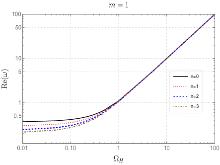
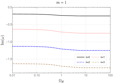
Figure 1: The dependence of real part $\omega_{R}$ (left plot) and imaginary part $\omega_{I}$ (right plot) of QNF on $\Omega_{H}$ for $m=1$. In each plot, we demonstrate four overtones from $n=0$ to $n=3$.

We demonstrate the numerical results of QNF for $m=5$ in Table. 2 and Fig. 2, and for $m=10$ in Table. 3 and Fig. 3. The behaviors of the QNF in this two cases are qualitatively similar to that of case $m=1$, except that for these higher values of $m$, $\omega_{R}$ is much more sensitive to the changes in $\Omega_{H}$, which also leads to a slightly larger amplitude of variation in $\omega_{I}$. While for the fundamental mode, the imaginary part still remains as the least susceptible to the changes in angular velocity. Interestingly, from the tables, we can observe that the differences in $\Omega_{I}$ between adjacent overtones get close to $\Delta\omega_{I}\approx 0.5$ as what we have found in case of $m=1$. By summarizing the QNF in the three specific cases of positive $m$, we may conclude that the qualitative features of QNF discovered presently are consistent across all positive values of $m$.

$m=5$

$n$	Method	$\Omega_{H}=0$	$\Omega_{H}=0.5$	$\Omega_{H}=1$	$\Omega_{H}=5$	$\Omega_{H}=10$
$0$	AIM	$1.92059-0.192507i$	$3.45759-0.223514i$	$5.57214-0.238330i$	$25.1239-0.249380i$	$50.0621-0.249844i$
	CFM	$1.92059-0.192507i$	$3.45759-0.223514i$	$5.57214-0.238330i$	$25.1239-0.249380i$	$50.0621-0.249844i$
$1$	AIM	$1.89952-0.580296i$	$3.44961-0.671489i$	$5.56945-0.715239i$	$25.1239-0.748142i$	$50.0621-0.749531i$
	CFM	$1.89952-0.580296i$	$3.44961-0.671489i$	$5.56945-0.715239i$	$25.1239-0.748142i$	$50.0621-0.749531i$
$2$	AIM	$1.85899-0.976231i$	$3.43424-1.12220i$	$5.56421-1.19288i$	$25.1238-1.24691i$	$50.0621-1.24922i$
	CFM	$1.85899-0.976232i$	$3.43424-1.12219i$	$5.56421-1.19288i$	$25.1238-1.24691i$	$50.0621-1.24922i$
$3$	AIM	$1.80226-1.38504i$	$3.41251-1.57715i$	$5.55664-1.67167i$	$25.1237-1.74568i$	$50.0621-1.74891i$
	CFM	$1.80226-1.38505i$	$3.41251-1.57716i$	$5.55664-1.67167i$	$25.1237-1.74568i$	$50.0621-1.74891i$

Table 2: The first four overtones $n=0,1,2,3$ of QNF at $m=5$ for different $\Omega_{H}$. The numerical results obtained by AIM and CFM.

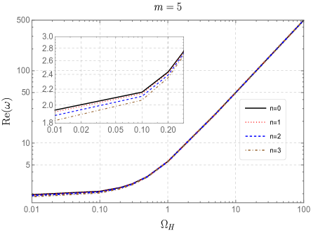
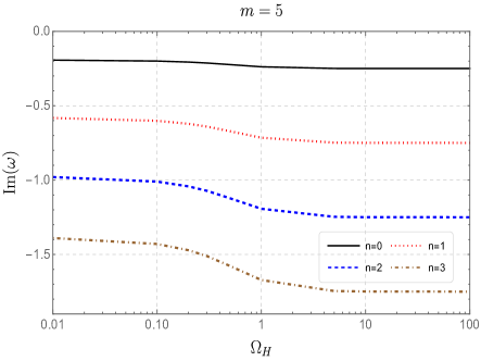
Figure 2: The dependence of real part $\omega_{R}$ (left plot) and imaginary part $\omega_{I}$ (right plot) of QNF on $\Omega_{H}$ for $m=5$. In each plot, we demonstrate four overtones from $n=0$ to $n=3$.

$m=10$

$n$	Method	$\Omega_{H}=0$	$\Omega_{H}=0.5$	$\Omega_{H}=1$	$\Omega_{H}=5$	$\Omega_{H}=10$
$0$	AIM	$3.84704-0.192464i$	$6.92012-0.223568i$	$11.1480-0.238370i$	$50.2488-0.249383i$	$100.125-0.249844i$
	CFM	$3.84704-0.192464i$	$6.92012-0.223568i$	$11.1480-0.238370i$	$50.2488-0.249383i$	$100.125-0.249844i$
$1$	AIM	$3.83639-0.578090i$	$6.91609-0.670944i$	$11.1467-0.715172i$	$50.2487-0.748148i$	$100.125-0.749532i$
	CFM	$3.83639-0.578090i$	$6.91609-0.670944i$	$11.1467-0.715172i$	$50.2487-0.748148i$	$100.125-0.749532i$
$2$	AIM	$3.81528-0.965797i$	$6.90811-1.11903i$	$11.1440-1.19216i$	$50.2487-1.24691i$	$100.125-1.24922i$
	CFM	$3.81528-0.965797i$	$6.90811-1.11903i$	$11.1440-1.19216i$	$50.2487-1.24691i$	$100.125-1.24922i$
$3$	AIM	$3.78412-1.35694i$	$6.89632-1.56828i$	$11.1400-1.66946i$	$50.2486-1.74568i$	$100.125-1.74891i$
	CFM	$3.78412-1.35694i$	$6.89632-1.56828i$	$11.1400-1.66946i$	$50.2486-1.74568i$	$100.125-1.74891i$

Table 3: The first four overtones $n=0,1,2,3$ of QNF at $m=10$ for different $\Omega_{H}$. The numerical results obtained by AIM and CFM.

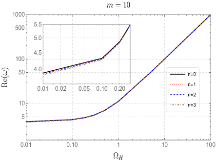
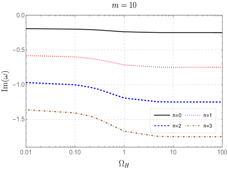
Figure 3: The dependence of real part $\omega_{R}$ (left plot) and imaginary part $\omega_{I}$ (right plot) of QNF on $\Omega_{H}$ for $m=10$. In each plot, we demonstrate four overtones from $n=0$ to $n=3$.

After discussing the properties of QNF with positive $m$, now we turn to the case of negative $m$. However, in this scenario, our numerical methods limit us to sufficiently large $|m|$ and small $\Omega_{H}$ (we take $0\leqslant\Omega_{H}\leqslant 10$), otherwise, we cannot obtain reliable numerical results. Therefore, we take $m=-10$ as an example to illustrate the characteristics of QNF for a negative winding number. On the other hand, in this situation, CFM is not working well, and we resort to six order WKB approximation method, which turns out to yield credible QNF, as demonstrated in Table. 4 and Fig. 4. Interestingly, a remarkably different QNF behaviors from what we have discussed for positive $m$ cases can be directly observed in the plots, although some common characteristics remain untouched, such as for a fixed $\Omega_{H}$, $\omega_{R}$ is only mildly decreased by increasing overtone number $n$, while $\omega_{I}$ suffers a considerable change. On the contrary to the QNF with $m>0$, where $\omega_{R}$ grows with angular velocity, in present case, $\omega_{R}$ rapidly drops off when increasing $\Omega_{H}$. For $\omega_{I}$, it is now sensitive to the changes in $\Omega_{H}$, rather than being insensitive as in positive $m$ case. With the increase of $\Omega_{H}$, the $\omega_{I}$ of all overtones grows and appears to converge to a small constant instead of approaching $|\Delta\omega_{I}|\approx 0.5$ between two adjacent overtones in the $m>0$ case. This result may suggest the existence of arbitrarily long-lived QNMs which is also called quasi-resonances Churilova:2019qph ; Konoplya:2004wg ; Ohashi:2004wr when angular velocity is large enough.

$m=-10$

$n$	Method	$\Omega_{H}=0$	$\Omega_{H}=0.5$	$\Omega_{H}=1$	$\Omega_{H}=5$	$\Omega_{H}=10$
$0$	AIM	$3.84704-0.192464i$	$2.32298-0.154473i$	$1.61296-0.122871i$	$0.452634-0.0422895i$	$0.237420-0.0229599i$
	WKB	$3.84704-0.192464i$	$2.32298-0.154473i$	$1.61296-0.122871i$	$0.452634-0.0422895i$	$0.237419-0.0229592i$
$1$	AIM	$3.83639-0.578090i$	$2.30553-0.464301i$	$1.59347-0.369216i$	$0.441756-0.126690i$	$0.231175-0.0687129i$
	WKB	$3.83639-0.57809i$	$2.30553-0.464299i$	$1.59347-0.369218i$	$0.441726-0.126693i$	$0.231032-0.0687109i$
$2$	AIM	$3.81528-0.965797i$	$2.27068-0.776801i$	$1.55434-0.617420i$	$0.419853-0.210568i$	$0.221032-0.114104i$
	WKB	$3.81528-0.965797i$	$2.27068-0.776713i$	$1.55429-0.617518i$	$0.419159-0.21071i$	$0.217909-0.114019i$
$3$	AIM	$3.78412-1.35694i$	$2.21860-1.09386i$	$1.49528-0.868883i$	$0.384825-0.294278i$	$0.214708-0.164592i$
	WKB	$3.78412-1.35694i$	$2.2185-1.09286i$	$1.49451-0.869833i$	$0.381929-0.295194i$	$0.19664-0.159081i$

Table 4: The first four overtones $n=0,1,2,3$ of QNF at $m=-10$ for different $\Omega_{H}$. The numerical results are obtained by AIM and WKB.

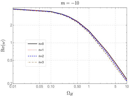
Figure 4: The dependence of real part $\omega_{R}$ (left plot) and imaginary part $\omega_{I}$ (right plot) of QNF on $\Omega_{H}$ for $m=-10$. In each plot, we demonstrate four overtones from $n=0$ to $n=3$.

It is natural and necessary to investigate how the QNF is affected by the winding number $m$. To this end, we separately compare $\omega_{R}$ and $\omega_{I}$ between different values of $m$ in Fig. 5 and Fig. 6, respectively. First of all, we observe that the four plots corresponding to four overtones in Fig. 5 appear almost identical, this is attributed to the fact that $\omega_{R}$ is weakly dependent on overtone number. Among the positive values of $m$, it is shown that for any given $\Omega_{H}$, a larger $m$ is always associated with a higher $\omega_{R}$, indicating a higher oscillation frequency of QNMs. At low values of $\Omega_{H}$, $\omega_{R}$ remains almost constant over a small range and then starts to increase slowly. After a certain value of $\Omega_{H}$ (looks like this value is lightly influenced by $m$), the rate of increase in $\omega_{R}$ becomes much more pronounced, showing a roughly linear relationship on these log-log plots, which implies a power law dependence of $\omega_{R}$ on $\Omega_{H}$. Note that all the curves are almost parallel to each other, which suggests that the slope is approximately free of $m$. By reading the tick marks of the log-log plots, we can get the value of slope for any overtone number $n$ at a large $\Omega_{H}$

$$\frac{\Delta\ln\omega_{R}}{\Delta\ln\Omega_{H}}\approx 1,$$ (41)

which directly leads to

$$\ln\omega_{R}\backsimeq\ln\Omega_{H}+\ln C_{m}$$ (42)

By taking $\Omega_{H}=1$, the $m$ dependent constant $C_{m}$ is determined to be $C_{m}\approx m$, such that we have

$$\omega_{R}\backsimeq m\Omega_{H},\quad m>0\,\text{and}\,\Omega_{H}\to+\infty.$$ (43)

For a negative winding number, the behavior of QNF diverges significantly from that observed with a positive $m$, as the corresponding $\omega_{R}$ monotonously decreases when $\Omega_{H}$ grows and manifests an opposite development to positive winding number case, which indicates a pronounced dependence of $\omega_{R}$ on both the sign and magnitude of winding number $m$. At a specified value of $m$, $\omega_{R}$ for $-|m|$ keeps to be smaller than that for $|m|$ while they start off at the same value related to $\Omega_{H}=0$, at which the generalized potential $U(\omega,r)$ depends on $m^{2}$ such that $\pm m$ will give rise to identical QNF.

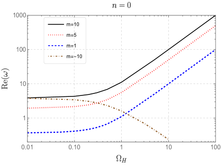
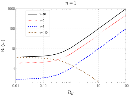
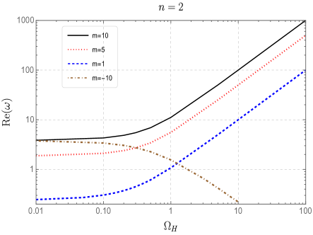
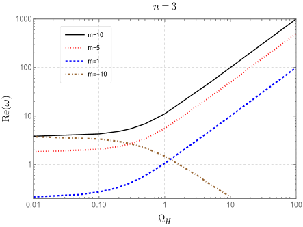
Figure 5: The separate comparison of real part $\omega_{R}$ of overtones from $n=0$ to $3$ between different $m$.

We now turn our attention to Fig. 6, which exhibits the comparisons of $\omega_{I}$ between different $m$. One can see that $\omega_{I}$ for all positive $m$ follows a consistent trend. As with the increase of $\Omega_{H}$, $\omega_{I}$ for $m>0$ starts to decrease and eventually converges to a certain value determined by the overtone number $n$. Naturally, a higher $n$ always gives rise to a greater magnitude of this asymptotic value of $\omega_{I}$. Before the convergence, some other distinctions arising from different $n$ are identified. For the fundamental modes ($n=0$), all the curves of $\omega_{I}$ for positive $m$ coincide with each other and this poses a striking contrast with the other plots of higher overtones. This alignment implies that changes in $m$ within the region of $m>0$ have ignorable impacts on $\omega_{I}$ for fundamental modes. However, for higher overtones, the impacts of positive $m$ show up in the way of inducing deviations of $\omega_{I}$ among varying $m$ at low values of $\Omega_{H}$. The most significant effects of $m$ is that the curves of $m=1$ is noticeably departed from the curves for $m=5$ and $m=10$. For the latter two $m$, a divergence is also formed, just the scale is markedly smaller than previous one. Generally, all the deviations in $\omega_{I}$ arising from $m$ are amplified by increasing $n$. This accentuation reveals that among positive $m$, at low values of $\Omega_{H}$, a higher $m$ will lead to a more negative $\omega_{I}$, indicating a longer life for QNMs, although this distinction will be eventually eliminated when $\Omega_{H}$ becomes large. The behaviors of curves for $m<0$ presents a striking contrast compared to the case of positive $m$. When raising $\Omega_{H}$, it is observed that the curves for $m>0$ have a downward trend, while for $m<0$, the curves have an upward trend. Recall that a similar opposite behavior of curves between positive and negative $m$ has also been revealed for $\omega_{R}$ in Fig. 5. The contrary behaviors of $\omega_{I}$ between positive and negative $m$, together with the fact that the generalized potential $U(\omega,r)$ is an even function in terms of $m$ at $\Omega_{H}=0$, such that $\pm m$ has exactly the same QNF and a larger positive $m$ corresponds to a larger $\omega_{I}$, all these facts finally help us predict that $\omega_{I}$ for $m=-10$ must be the mode that remains the highest $\omega_{I}$ among all the value of $m$ considered here in the whole range of $\Omega_{H}$, as depicted in this figure. This result suggests that employing a perturbation optical field with a negative winding number $m$ is preferable for maximizing the lifespan of QNMs.

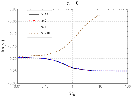
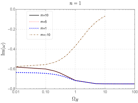
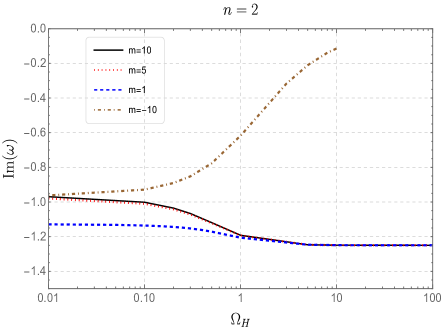
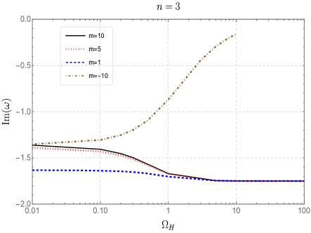
Figure 6: The comparison of imaginary part $\omega_{I}$ of QNF between different $m$, and each plot corresponds to one certain overtone number $n$.

V Conclusions and Discussions

In this paper, we have performed an investigation of the dynamical characteristics of the analog rotating black hole in the photon-fluid model. Naturally, these dynamical properties manifest themselves through QNMs, prompting us to calculate the QNF accordingly. To ensure the reliability of our results, we employed three numerical methods for calculating the QNFs. Besides the fundamental modes, the overtones are also calculated up to $n=3$ with the intention of acquiring more information of the QNMs. We separately discussed the QNF for $m>0$ and $m<0$.

For $m>0$, we find that the real part $\omega_{R}$ of QNF for all the overtone number is sensitive to the angular velocity $\Omega_{H}$ and increases monotonically with the grow of $\Omega_{H}$, indicating a black hole spinning faster can support QNMs with higher oscillation frequencies. Conversely, for the imaginary part $\omega_{I}$ of QNF, its behavior diverges from that of $\omega_{R}$. With an increase in $\Omega_{H}$, we find that $\omega_{I}$ is insensitive to $\Omega_{H}$ and it monotonically decreases for a while and then eventually approaches a certain negative constant whose value is $n$-dependent. Note that a concern arises due to the unlimited angular velocity may cause positive $\omega_{I}$ implying unstable QNMs, while this concern has been addressed by our numerical results that $\omega_{I}$ remains negative for any arbitrarily large $\Omega_{H}$. Additionally, while $\omega_{R}$ is found to be weakly dependent on the overtone number $n$, $\omega_{I}$ exhibits a strong correlation on $n$. With a higher $n$, $\omega_{R}$ only mildly drops off and $\omega_{I}$ experiences a notable reduction. When $\Omega_{H}$ is large, $\omega_{R}$ displays a approximately linear dependence on $m\Omega_{H}$, and for neighboring two $\omega_{I}$ we have $|\Delta\omega_{I}|\approx 0.5$. Further more, we find that a larger winding number can increase both $\omega_{R}$ and $\omega_{I}$, as $\omega_{R}\backsimeq m\Omega_{H}$ for $m>0\,\text{and}\,\Omega_{H}\to+\infty$. However, $\omega_{R}$ is notably improved by $m$, whose impacts on $\omega_{I}$ is slight especially for the fundamental mode. An interesting observation is that, the winding number $m$ has noticeable effects on $\omega_{R}$ but only tiny impacts on $\omega_{I}$, whereas the overtone number $n$ can only cause mild modifications to $\omega_{R}$ but notable effects on $\omega_{I}$. This illustrates that $m$ and $n$ exert opposite influences to QNF.

For $m<0$, strikingly contrasting behaviors of QNF have been observed in comparison to the case of $m>0$. Specifically, as $\Omega_{H}$ increases, $\omega_{R}$ will be monotonically decreased while $\omega_{I}$ exhibits a continuous increase. The $\omega_{R}$ for different overtones decreases with almost the same rate, but for $\omega_{I}$, a higher overtone demonstrates a notable larger rate of increase, as illustrated in the corresponding semi-log plot. At high value of $\Omega_{H}$, all the overtones of $\omega_{I}$ seem to have trend to converge towards a common certain constant which is close to zero, deviating the relation of $|\Delta\omega_{I}|\approx 0.5$ for $m>0$, but instead converting to $|\Delta\omega_{I}|\approx 0$. This trend towards zero for $\omega_{I}$ suggests the possible existence of arbitrarily long-lived QNMs, also referred to as quasi-resonances. Considering that when $\Omega_{H}=0$, the generalized potential $U(\omega,r)$ is an even function in terms of $m$, such that QNF for $\pm|m|$ is expected to be identical at $\Omega_{H}=0$. On the other hand, we have known that when $\Omega_{H}$ becomes larger the $\omega_{R}$ will decrease. Considering these two observations together, one can easily predict a relation $\omega_{R,-|m|}<\omega_{R,|m|}$ for $m\neq 0$, and the same reasoning can also be applied to $\omega_{I}$ to get $\omega_{I,-|m|}>\omega_{I,|m|}$. This simple prediction has been proven in Fig. 5 and Fig. 6, respectively. Consequently, to achieve longer-lived QNMs which brings some convenience for observing, the fluctuating optical field used for generating QNMs should ideally possess a negative winding number $m<0$.

Black hole physics is indisputably important in the modern physics, especially in the attempts of advancing our understanding of quantum gravity theory. Over the past century, black holes have attracted significant attentions, but almost all the researches are limited in theoretical side, due to the extreme hardship of observing the actual black holes in astrophysical environments. Even if we have detected astrophysical black holes trough gravitational waves, some intriguing effects of black holes, such as Hawking radiation, may still be too faint to be directly detected by current cutting-edge technology of human beings. In light of this, simulating analog black holes in laboratory settings seems like a concession to practical limitations, it indeed has proven useful and enlightening in enhancing our comprehension of black hole physics, even including aspects of quantum gravity Braunstein:2023jpo . Particularly, it is worth noting that the recent exciting advancements in Svancara:2023yrf which reported observations of bound states and distinctive analog black hole ringdown signatures in an analog rotating curved spacetime from a giant quantum vortex, indeed brings us a more promising future of studying physics in the black holes spacetime by analogy. As for our present work, we analyzed the properties of QNMs for the analog black holes in a photon-fluid model, which has been experimentally constructed Vocke2018 . Therefore, with these experimental advancements, we are optimistic that the QNMs we have investigated here will soon be observable in apparatus of this photon-fluid model by which provides a novel testbed to black hole physics and theories of gravitation.

Appendix A The Connection between Photon-Fluid and Analogue Black Holes

We give a sketch of how to derive the black hole metric in nonlinear optical system. As we have mentioned previously, this derivation has been discussed in PhysRevA.78.063804 ; Ciszak:2021xlw , while in this Appendix, our purpose is to make a more detailed and concrete discussion on the construction of the analogue rotating black hole spacetime in this optical field system.

To understand how the analogue black hole spacetime is constructed, the starting point is to see what we can get from the hydromechanics. An insightful discovery by Unruh Unruh:1980cg ; Unruh:1994je is that an analogue black hole spacetime can be built from the following fundamental equations

$$\partial_{t}\rho+\nabla\cdot(\rho\,\mathbf{v})=0,\quad\quad\text{Equation of continuity,}$$ (44a)

$$\rho\frac{d\mathbf{v}}{dt}\equiv\rho\left[\partial_{t}\mathbf{v}+(\mathbf{v}\cdot\nabla)\mathbf{v}\right]=\mathbf{f},\quad\quad\text{ Euler's equation,}$$ (44b)

which describe the dynamics of fluids. In this equation, $\rho$ is the density of the fluids and we have used boldface to denote the fluids velocity vector $\mathbf{v}$ and the force vector $\mathbf{f}$ acted on the fluids. So the Euler equation is just equivalent to Newton’s second law $\mathbf{f}=m\,\mathbf{a}$ with $\mathbf{f}$ being the force applied to a small lumps of the fluid.

We now focus on the Euler’s equation. From the knowledge of the vector analysis, we have identity

$$\mathbf{v}\times(\nabla\times\mathbf{v})=\frac{1}{2}\nabla v^{2}-(\mathbf{v}\cdot\nabla)\mathbf{v},$$ (45)

where $v^{2}=\mathbf{v}\cdot\mathbf{v}$. By assuming the fluid to be inviscid (zero viscosity) which means that the only forces present being those due to pressure $p$. Then for the force density, we have

$$\mathbf{f}=-\nabla p.$$ (46)

With these conditions, we have the following Euler’s equation

$$\partial_{t}\mathbf{v}=\mathbf{v}\times(\nabla\times\mathbf{v})-\frac{1}{2}\nabla v^{2}-\frac{\nabla p}{\rho}.$$ (47)

Furthermore, we assume that the fluids is locally irrotational which directly leads to $\nabla\times\mathbf{v}=0$ (vorticity free), and it implies that the velocity vector is the gradient of some scalar $\phi$, i.e. $\mathbf{v}=-\nabla\phi$. On the other hand, we also require the fluid to be barotropic which means that the density $\rho$ is a function of pressure $p$ only, such that it is possible to define a function $h(p)$ as

$$h(p)=\int_{0}^{p}\frac{dp^{\prime}}{\rho(p^{\prime})}=\int_{x(0)}^{x(p)}\frac{\nabla p^{\prime}\cdot d\mathbf{x}}{\rho(p^{\prime})}=\int_{x(0)}^{x(p)}\nabla h(p^{\prime})\cdot d{\mathbf{x}},$$ (48)

which shows that

$$\nabla h=\frac{\nabla p}{\rho}.$$ (49)

For more details, one can refer to Barcelo:2005fc to have a comprehensive understanding on analogue gravity and the prodedures of the derivation of black hole metric from Eq. (44).

The starting point of finding a black hole metric in optical system is from the equation which describes the slowly varying envelope of the optical field. The dynamics of the photon-fluid in our consideration is governed by the nonlinear Schrödinger equation (NSE)

$$\frac{\partial E}{\partial z}=\frac{i}{2k}\nabla^{2}E-i\frac{kn_{2}}{n_{0}}E|E|^{2},$$ (50)

where $z$ is the propagation direction, $|E|^{2}$ is the optical field intensity and $\nabla^{2}E$ is defined with respect to the transverse coordinates $(x,y)$, $i$ is the imaginary unit, $k=2\pi n_{0}/\lambda$ is the wave number, $\lambda$ is the laser wavelength in vacuum, $n_{0}$ is the linear refractive index, $n_{2}>0$ is the material nonlinear coefficient which characterizes the intensity dependent refractive index $n=n_{0}-n_{2}|E|^{2}$ of the self-defocusing media. As a consequence, light propagating in a self-defocusing medium induces a local negative bending of the refractive index which, in turn, affects the light beam itself. At a microscopic level this can be described in terms of an atom-mediated repulsive interaction between photons which leads to the formation of a “photon fluid”, such that we get a flavor of fluids in optical system here.

We now start to reveal the hidden links between Eq. (50) describing optical field and Eq. (44) describing fluids dynamics. The first step in this task is to apply the Madelung transformation to write the complex EM field $E$ in terms of its amplitude and phase

$$E=\rho^{\frac{1}{2}}e^{i\phi},$$ (51)

and by this formula of $E$, we would like to investigate Eq. (50) term by term. The term on the left hand side is expressed as

$$\partial_{z}E=\partial_{z}(\rho^{\frac{1}{2}}e^{i\phi})=i\rho^{\frac{1}{2}}e^{i\phi}\partial_{z}\phi+\frac{1}{2}\rho^{-\frac{1}{2}}e^{i\phi}\partial_{z}\rho.$$ (52)

The first term on the righthand side is

$$\begin{split}\nabla^{2}E&=\nabla^{2}(\rho^{\frac{1}{2}}e^{i\phi})=\rho^{\frac{1}{2}}\nabla^{2}e^{i\phi}+2\nabla\rho^{\frac{1}{2}}\cdot\nabla e^{i\phi}+e^{i\phi}\nabla^{2}\rho^{\frac{1}{2}}\\ &=\rho^{\frac{1}{2}}e^{i\phi}(i\nabla^{2}\phi-(\nabla\phi)^{2})+i\rho^{-\frac{1}{2}}e^{i\phi}\nabla\rho\cdot\nabla\phi+e^{i\phi}\nabla^{2}\rho^{\frac{1}{2}}\\ &=\frac{1}{\alpha}ie^{i\phi}\rho^{-\frac{1}{2}}[\nabla\rho\cdot\nabla(\alpha\phi)+\rho\nabla^{2}(\alpha\phi)]-\frac{1}{\alpha^{2}}\rho^{\frac{1}{2}}e^{i\phi}(\nabla(\alpha\phi))^{2}+e^{i\phi}\nabla^{2}\rho^{\frac{1}{2}}\\ &=\frac{1}{\alpha}ie^{i\phi}\rho^{-\frac{1}{2}}\nabla\cdot(\rho\mathbf{v})-\frac{1}{\alpha^{2}}\rho^{\frac{1}{2}}e^{i\phi}\mathbf{v}^{2}+e^{i\phi}\nabla^{2}\rho^{\frac{1}{2}},\end{split}$$ (53)

where we have defined “fluids” velocity $\mathbf{v}=\alpha\nabla\phi\equiv\nabla\psi$ and $\alpha=\frac{c}{kn_{0}}$ (here $c$ is the speed of the light). The last term on righthand side is

$$E|E|^{2}=\rho^{\frac{3}{2}}e^{i\phi}.$$ (54)

We substitute these obtained equations in Eq. (50) and we get a pair of equations

$$\frac{1}{2}\rho^{-\frac{1}{2}}e^{i\phi}\partial_{z}\rho=-\frac{1}{2\alpha k}\rho^{-\frac{1}{2}}e^{i\phi}\nabla\cdot(\rho\mathbf{v})$$ (55)

$$i\rho^{\frac{1}{2}}e^{i\phi}\partial_{z}\phi=\frac{i}{2k}\left[-\frac{1}{\alpha^{2}}\rho^{\frac{1}{2}}e^{i\phi}\mathbf{v}^{2}+e^{i\phi}\nabla^{2}\rho^{\frac{1}{2}}\right]-i\frac{kn_{2}}{n_{0}}\rho^{\frac{3}{2}}e^{i\phi},$$ (56)

The Eq. (55) leads to

$$k\alpha\frac{\partial\rho}{\partial z}+\nabla\cdot(\rho\mathbf{v})=\frac{c}{n_{0}}\frac{\partial\rho}{\partial z}+\nabla\cdot(\rho\mathbf{v})=0.$$ (57)

Eq. (56) leads to

$$\frac{c}{n_{0}}\frac{\partial(\alpha\phi)}{\partial z}+\frac{1}{2}\mathbf{v}^{2}-\frac{\alpha^{2}}{2}\frac{\nabla^{2}\rho^{\frac{1}{2}}}{\rho^{\frac{1}{2}}}+\frac{k^{2}\alpha^{2}n_{2}}{n_{0}}\rho=0.$$ (58)

We define $t=\frac{n_{0}}{c}z$ and note that $\psi=\alpha\phi$, which results in

$$\frac{\partial\rho}{\partial t}+\nabla\cdot(\rho\mathbf{v})=0,$$ (59)

$$\frac{\partial\psi}{\partial t}+\frac{1}{2}\mathbf{v}^{2}+\frac{c^{2}n_{2}}{n_{0}^{3}}\rho-\frac{1}{2}\frac{c^{2}}{k^{2}n_{0}^{2}}\frac{\nabla^{2}\rho^{\frac{1}{2}}}{\rho^{\frac{1}{2}}}=0.$$ (60)

Eq. (59) is just the equation of continuity which is in exact the same form as that in fluids dynamics, and Eq. (60) is the Euler’s equation. The last term in Eq. (60) represents quantum pressure which has no analogy in classical fluid dynamics. In optics, it is a direct consequence of the wave nature of light (it arises from the diffraction term $\nabla^{2}E$) and is significant in rapidly varying and/or low-intensity regions such as dark-soliton cores and close to boundaries.

When the quantum pressure is negligible, then Eq. (60) has the exact same form of the Euler’s equation for fluid dynamics. By comparison, it is clear to see that $h(p(\rho))\equiv\frac{c^{2}n_{2}}{n_{0}^{3}}\rho$, and take Eq. (49) into consideration, we can get the relation between $p$ and $\rho$,

$$P=\frac{c^{2}n_{2}\rho^{2}}{2n_{0}^{3}},$$ (61)

such that the speed of sound $c_{s}$ can be obtained as

$$c_{s}^{2}=\frac{\partial P}{\partial\rho}\bigg{|}_{\rho=\rho_{0}}=\frac{c^{2}n_{2}\rho_{0}}{n_{0}^{3}}.$$ (62)

As we have obtained the same equation of continuity and Euler’s equation in optical system as that in hydromechanics, the connections between the photon-fluid and the analog gravity is clear now, since these two fundamental equations are the starting point of constructing analog gravity in fluids.

References

- (1) LIGO Scientific, Virgo collaboration, B. P. Abbott et al., Tests of general relativity with GW150914, Phys. Rev. Lett. 116 (2016) 221101, [1602.03841].
- (2) LIGO Scientific, Virgo collaboration, B. P. Abbott et al., Properties of the Binary Black Hole Merger GW150914, Phys. Rev. Lett. 116 (2016) 241102, [1602.03840].
- (3) LIGO Scientific, Virgo collaboration, B. P. Abbott et al., GWTC-1: A Gravitational-Wave Transient Catalog of Compact Binary Mergers Observed by LIGO and Virgo during the First and Second Observing Runs, Phys. Rev. X 9 (2019) 031040, [1811.12907].
- (4) Event Horizon Telescope collaboration, K. Akiyama et al., First M87 Event Horizon Telescope Results. IV. Imaging the Central Supermassive Black Hole, Astrophys. J. Lett. 875 (2019) L4, [1906.11241].
- (5) Event Horizon Telescope collaboration, K. Akiyama et al., First M87 Event Horizon Telescope Results. VI. The Shadow and Mass of the Central Black Hole, Astrophys. J. Lett. 875 (2019) L6, [1906.11243].
- (6) Event Horizon Telescope collaboration, K. Akiyama et al., First Sagittarius A* Event Horizon Telescope Results. I. The Shadow of the Supermassive Black Hole in the Center of the Milky Way, Astrophys. J. Lett. 930 (2022) L12, [2311.08680].
- (7) W. G. Unruh, Experimental black hole evaporation, Phys. Rev. Lett. 46 (1981) 1351–1353.
- (8) W. G. Unruh, Sonic analog of black holes and the effects of high frequencies on black hole evaporation, Phys. Rev. D 51 (1995) 2827–2838, [gr-qc/9409008].
- (9) P. Švančara, P. Smaniotto, L. Solidoro, J. F. MacDonald, S. Patrick, R. Gregory et al., Rotating curved spacetime signatures from a giant quantum vortex, Nature 628 (2024) 66–70, [2308.10773].
- (10) O. Lahav, A. Itah, A. Blumkin, C. Gordon and J. Steinhauer, Realization of a sonic black hole analogue in a Bose-Einstein condensate, Phys. Rev. Lett. 105 (2010) 240401, [0906.1337].
- (11) J. R. Muñoz de Nova, K. Golubkov, V. I. Kolobov and J. Steinhauer, Observation of thermal Hawking radiation and its temperature in an analogue black hole, Nature 569 (2019) 688–691, [1809.00913].
- (12) M. Isoard and N. Pavloff, Departing from thermality of analogue Hawking radiation in a Bose-Einstein condensate, Phys. Rev. Lett. 124 (2020) 060401, [1909.02509].
- (13) M. A. Anacleto, F. A. Brito, C. V. Garcia, G. C. Luna and E. Passos, Quantum-corrected rotating acoustic black holes in Lorentz-violating background, Phys. Rev. D 100 (2019) 105005, [1904.04229].
- (14) R. Balbinot, A. Fabbri, R. A. Dudley and P. R. Anderson, Particle Production in the Interiors of Acoustic Black Holes, Phys. Rev. D 100 (2019) 105021, [1910.04532].
- (15) G. Eskin, Hawking type radiation from acoustic black holes with time-dependent metric, Reports on Mathematical Physics 88 (2021) 161–174.
- (16) M. Visser, Acoustic black holes: Horizons, ergospheres, and Hawking radiation, Class. Quant. Grav. 15 (1998) 1767–1791, [gr-qc/9712010].
- (17) E. Berti, V. Cardoso and J. P. S. Lemos, Quasinormal modes and classical wave propagation in analogue black holes, Phys. Rev. D 70 (2004) 124006, [gr-qc/0408099].
- (18) V. Cardoso, J. P. S. Lemos and S. Yoshida, Quasinormal modes and stability of the rotating acoustic black hole: Numerical analysis, Phys. Rev. D 70 (2004) 124032, [gr-qc/0410107].
- (19) R. G. Daghigh and M. D. Green, High Overtone Quasinormal Modes of Analog Black Holes and the Small Scale Structure of the Background Fluid, Class. Quant. Grav. 32 (2015) 095003, [1411.7066].
- (20) T. Torres, S. Patrick, M. Richartz and S. Weinfurtner, Quasinormal Mode Oscillations in an Analogue Black Hole Experiment, Phys. Rev. Lett. 125 (2020) 011301, [1811.07858].
- (21) M. J. Jacquet, L. Giacomelli, Q. Valnais, M. Joly, F. Claude, E. Giacobino et al., Quantum Vacuum Excitation of a Quasinormal Mode in an Analog Model of Black Hole Spacetime, Phys. Rev. Lett. 130 (2023) 111501, [2110.14452].
- (22) S. Patrick, Quasinormal modes in dispersive black hole analogues, 2007.06671.
- (23) S. Basak and P. Majumdar, ‘Superresonance’ from a rotating acoustic black hole, Class. Quant. Grav. 20 (2003) 3907–3914, [gr-qc/0203059].
- (24) M. Richartz, S. Weinfurtner, A. J. Penner and W. G. Unruh, General universal superradiant scattering, Phys. Rev. D 80 (2009) 124016, [0909.2317].
- (25) M. A. Anacleto, F. A. Brito and E. Passos, Superresonance effect from a rotating acoustic black hole and Lorentz symmetry breaking, Phys. Lett. B 703 (2011) 609–613, [1101.2891].
- (26) S. Patrick and S. Weinfurtner, Superradiance in dispersive black hole analogues, Phys. Rev. D 102 (2020) 084041, [2007.03769].
- (27) H.-H. Zhao, G.-L. Li and L.-C. Zhang, Generalized uncertainty principle and entropy of three-dimensional rotating acoustic black hole, Phys. Lett. A 376 (2012) 2348–2351.
- (28) M. A. Anacleto, F. A. Brito, E. Passos and W. P. Santos, The entropy of the noncommutative acoustic black hole based on generalized uncertainty principle, Phys. Lett. B 737 (2014) 6–11, [1405.2046].
- (29) M. A. Anacleto, F. A. Brito, G. C. Luna, E. Passos and J. Spinelly, Quantum-corrected finite entropy of noncommutative acoustic black holes, Annals Phys. 362 (2015) 436–448, [1502.00179].
- (30) M. A. Anacleto, I. G. Salako, F. A. Brito and E. Passos, The entropy of an acoustic black hole in neo-Newtonian theory, Int. J. Mod. Phys. A 33 (2018) 1850185, [1603.07311].
- (31) B. Zhang, Thermodynamics of acoustic black holes in two dimensions, Adv. High Energy Phys. 2016 (2016) 5710625, [1606.00693].
- (32) Q.-B. Wang and X.-H. Ge, Geometry outside of acoustic black holes in ()-dimensional spacetime, Phys. Rev. D 102 (2020) 104009, [1912.05285].
- (33) X.-H. Ge and S.-J. Sin, Acoustic black holes for relativistic fluids, JHEP 06 (2010) 087, [1001.0371].
- (34) M. A. Anacleto, F. A. Brito and E. Passos, Acoustic Black Holes from Abelian Higgs Model with Lorentz Symmetry Breaking, Phys. Lett. B 694 (2011) 149–157, [1004.5360].
- (35) M. A. Anacleto, F. A. Brito and E. Passos, Supersonic Velocities in Noncommutative Acoustic Black Holes, Phys. Rev. D 85 (2012) 025013, [1109.6298].
- (36) M. A. Anacleto, F. A. Brito and E. Passos, Acoustic Black Holes and Universal Aspects of Area Products, Phys. Lett. A 380 (2016) 1105–1109, [1309.1486].
- (37) N. Bilic, Relativistic acoustic geometry, Class. Quant. Grav. 16 (1999) 3953–3964, [gr-qc/9908002].
- (38) S. Fagnocchi, S. Finazzi, S. Liberati, M. Kormos and A. Trombettoni, Relativistic Bose-Einstein Condensates: a New System for Analogue Models of Gravity, New J. Phys. 12 (2010) 095012, [1001.1044].
- (39) M. Visser and C. Molina-Paris, Acoustic geometry for general relativistic barotropic irrotational fluid flow, New J. Phys. 12 (2010) 095014, [1001.1310].
- (40) L. Giacomelli and S. Liberati, Rotating black hole solutions in relativistic analogue gravity, Phys. Rev. D 96 (2017) 064014, [1705.05696].
- (41) X.-H. Ge, M. Nakahara, S.-J. Sin, Y. Tian and S.-F. Wu, Acoustic black holes in curved spacetime and the emergence of analogue Minkowski spacetime, Phys. Rev. D 99 (2019) 104047, [1902.11126].
- (42) H. Guo, H. Liu, X.-M. Kuang and B. Wang, Acoustic black hole in Schwarzschild spacetime: quasi-normal modes, analogous Hawking radiation and shadows, Phys. Rev. D 102 (2020) 124019, [2007.04197].
- (43) C.-K. Qiao and M. Zhou, The gravitational bending of acoustic Schwarzschild black hole, Eur. Phys. J. C 83 (2023) 271, [2109.05828].
- (44) H. S. Vieira, K. Destounis and K. D. Kokkotas, Slowly-rotating curved acoustic black holes: Quasinormal modes, Hawking-Unruh radiation, and quasibound states, Phys. Rev. D 105 (2022) 045015, [2112.08711].
- (45) A. Ditta, T. Xia and M. Yasir, Particle motion and lensing with plasma of acoustic Schwarzschild black hole, Int. J. Mod. Phys. A 38 (2023) 2350041.
- (46) R. Ling, H. Guo, H. Liu, X.-M. Kuang and B. Wang, Shadow and near-horizon characteristics of the acoustic charged black hole in curved spacetime, Phys. Rev. D 104 (2021) 104003, [2107.05171].
- (47) N. U. Molla and U. Debnath, Gravitational Lensing of Acoustic Charged Black Holes, Astrophys. J. 947 (2023) 14.
- (48) C. Barcelo, S. Liberati and M. Visser, Analogue gravity, Living Rev. Rel. 8 (2005) 12, [gr-qc/0505065].
- (49) F. Marino, Acoustic black holes in a two-dimensional “photon fluid”, Phys. Rev. A 78 (Dec, 2008) 063804.
- (50) F. Marino, M. Ciszak and A. Ortolan, Acoustic superradiance from optical vortices in self-defocusing cavities, Phys. Rev. A 80 (Dec, 2009) 065802.
- (51) M. Ciszak and F. Marino, Acoustic black-hole bombs and scalar clouds in a photon-fluid model, Phys. Rev. D 103 (2021) 045004, [2101.07508].
- (52) D. Vocke, C. Maitland, A. Prain, K. E. Wilson, F. Biancalana, E. M. Wright et al., Rotating black hole geometries in a two-dimensional photon superfluid, Optica 5 (Sep, 2018) 1099–1103.
- (53) S. L. Braunstein, M. Faizal, L. M. Krauss, F. Marino and N. A. Shah, Analogue simulations of quantum gravity with fluids, Nature Rev. Phys. 5 (2023) 612–622, [2402.16136].
- (54) H.-P. Nollert, Quasinormal modes: the characteristic ‘sound’ of black holes and neutron stars, Classical and Quantum Gravity 16 (dec, 1999) R159.
- (55) R. A. Konoplya and A. Zhidenko, Quasinormal modes of black holes: From astrophysics to string theory, Rev. Mod. Phys. 83 (2011) 793–836, [1102.4014].
- (56) E. Berti, V. Cardoso and A. O. Starinets, Quasinormal modes of black holes and black branes, Class. Quant. Grav. 26 (2009) 163001, [0905.2975].
- (57) H. T. Cho, A. S. Cornell, J. Doukas, T. R. Huang and W. Naylor, A New Approach to Black Hole Quasinormal Modes: A Review of the Asymptotic Iteration Method, Adv. Math. Phys. 2012 (2012) 281705, [1111.5024].
- (58) E. W. Leaver, An analytic representation for the quasi-normal modes of kerr black holes, Proc. R. Soc. Lond. A 402 (1985) 285–298.
- (59) E. W. Leaver, Quasinormal modes of reissner-nordström black holes, Phys. Rev. D 41 (May, 1990) 2986–2997.
- (60) W. Gautschi, Computational aspects of three-term recurrence relations, SIAM Review 9 (1967) 24–82, [https://doi.org/10.1137/1009002].
- (61) R. A. Konoplya, A. Zhidenko and A. F. Zinhailo, Higher order WKB formula for quasinormal modes and grey-body factors: recipes for quick and accurate calculations, Class. Quant. Grav. 36 (2019) 155002, [1904.10333].
- (62) M. S. Churilova, R. A. Konoplya and A. Zhidenko, Arbitrarily long-lived quasinormal modes in a wormhole background, Phys. Lett. B 802 (2020) 135207, [1911.05246].
- (63) R. A. Konoplya and A. V. Zhidenko, Decay of massive scalar field in a Schwarzschild background, Phys. Lett. B 609 (2005) 377–384, [gr-qc/0411059].
- (64) A. Ohashi and M.-a. Sakagami, Massive quasi-normal mode, Class. Quant. Grav. 21 (2004) 3973–3984, [gr-qc/0407009].