CAVIAR: Categorical-Variable Embeddings for Accurate and Robust Inference
indentfirst=false, leftmargin=2em, rightmargin=2em, vskip=1ex
Anirban Mukherjee,1∗ Hannah H. Chang2
1Samuel Curtis Johnson Graduate School of Management, Cornell University,
Sage Hall, Ithaca, NY 14850, USA
2Lee Kong Chian School of Business, Singapore Management University,
50 Stamford Road, Singapore, 178899
∗To whom correspondence should be addressed; E-mail: am253@cornell.edu.
Abstract
Social science research often hinges on the relationship between categorical variables and outcomes. We introduce CAVIAR, a novel method for embedding categorical variables that assume values in a high-dimensional ambient space but are sampled from an underlying manifold. Our theoretical and numerical analyses outline challenges posed by such categorical variables in causal inference. Specifically, dynamically varying and sparse levels can lead to violations of the Donsker conditions and a failure of the estimation functionals to converge to a tight Gaussian process. Traditional approaches, including the exclusion of rare categorical levels and principled variable selection models like LASSO, fall short. CAVIAR embeds the data into a lower-dimensional global coordinate system. The mapping can be derived from both structured and unstructured data, and ensures stable and robust estimates through dimensionality reduction. In a dataset of direct-to-consumer apparel sales, we illustrate how high-dimensional categorical variables, such as zip codes, can be succinctly represented, facilitating inference and analysis.
Keywords: Causal Analysis, Categorical Variables, High Dimensional Inference, Sparse Data, Machine Learning, Econometrics.
Introduction
This paper addresses concerns related to the estimation of causal econometric models in the social sciences in which categorical variables, taking values in an ambient space and presumed to be sampled from an underlying manifold, are mapped to dependent variables of interest.
Distance within the manifold is considered a measure of similarity relevant to the analysis. For instance, when analyzing a categorical variable that describes color, distance may correspond to the light spectrum, such that bottle green is further from maroon than from turquoise. Similarly, when examining a spatial categorical variable, distance may relate to physical proximity, indicating that a city is closer to its suburb than to a distant location. When analyzing sound, distance may be related to frequencies, implying that the sounds of a viola and violin are more similar than those from a snare drum. In classical methods, distinct elements of the set are accorded distinct levels, such that each color, location, and instrument might have its own level in corresponding categorical variables.
Categorical variables often present two complexities: large and increasing cardinality with sample size (the categorical variable assumes many distinct levels, with new levels added as new samples are introduced) and sparsity (levels that correspond to only a few observations). These conditions may occur when specificity is desired. For instance, consider the categorization of religion—a typical covariate in the social sciences (Fox 2001, Woodberry 2012). When categorized broadly, a religion categorical variable may be developed to include only a few levels (e.g., Christianity, Islam, etc.).
However, when more granularity is desired, the categorical variable may encompass many distinct values (Center 2015, Finke and Stark 2005). For example, there may be thousands of denominations and sects, leading to a system that is both characterized by large cardinality and marked by sparsity, in the sense that, for many designations, a particular dataset may contain only one or a few observations (Smith 1990, Steensland et al. 2000). Moreover, as the data grows, observations may be added that pertain to more detailed sub-categories whose inclusion in the analysis as distinct levels may be desirable (Voas et al. 2013, Woodberry et al. 2012).
These issues complicate causal inference. Typically, a fixed effects model is specified whereby each level of the categorical variable is accorded its own parameter, which is then estimated freely; the traditional fixed-effects model is a non-parametric model. This methodology is ubiquitous and has been used countless times in the social sciences (Wooldridge 2010). It is robust and well-understood in cases where the categorical data exhibits low cardinality and high density of occurrence, which are the canonical scenarios for which it was originally proposed (Suits 1957).
In scenarios where the data exhibits high cardinality and sparsity, the canonical fixed effects model can break down, leading to inaccurate and imprecise inference. Here, we depart from existing studies by considering cases of extreme sparsity where a categorical variable may have thousands of possible levels conceptually (e.g., thousands of possible religious subdivisions), only a fraction of which may be represented in the data. In such cases, the categorical variable is effectively increasing in levels and dimensionality with the inclusion of more data. Additionally, our model maps onto situations where the context is dynamic, and therefore, the categorical variable is dynamic—over time, new category levels emerge (e.g., new religious sects are formed) and old category levels become irrelevant (e.g., extant religious sects become dormant). These considerations challenge prior econometric models, which were generally developed for scenarios where a categorical variable reflects a few fixed dimensionality categorical factors, such as might emerge from the use of a Likert scale in a survey.
To combat this issue, researchers often resort to ad-hoc solutions, such as collapsing rare levels into a ‘meta-level’ or applying formal regularization methods like the Least Absolute Shrinkage and Selection Operator (LASSO) to the indicator variables of the levels (Tutz and Gertheiss 2016). However, both approaches can lead to inaccurate and imprecise inference; this is because, in the fixed effects model, inference is only drawn from observations that relate to a specific level of the categorical variable. Consequently, the addition of levels to the categorical variable—whether as they appear in the data (the traditional model), when they occur a specified number of times (the ad-hoc solution), or when the fixed effect coefficient is ‘sufficiently’ large or the design matrix is ‘sufficiently’ non-singular (the regularized solution)—can result in violations of the Donsker conditions. This, in turn, eliminates the guarantee that the estimators, as functionals of the empirical process, will converge to a Brownian bridge.
Addressing this research gap, we propose a method for the development of a categorical variable embedding—an injunction from the high-dimensional ambient space to a single global coordinate system of lower dimensionality, where distance captures a notion of similarity in the categorical levels, such that the location of each level can act as a data feature in the causal model. Fixed effects in the original causal model are recovered through their projection onto the lower-dimensional space.
Our underlying research agenda speaks to the development of a data pipeline that averts issues linked to categorical variable cardinality and sparsity. In relatively straightforward cases, our method echoes the intuition of replacing the fixed effects with a structural model of explanatory variables. Unlike previous approaches that require a hierarchical structure (Carrizosa et al. 2022) or specific latent matrix factorizations (Cerda and Varoquaux 2020), our approach is amenable to the inclusion of group-level structured and unstructured data, with the latter being an important novelty given the prevalence and availability of high quality pre-trained embeddings. In such cases, the method adopts the lens of first developing features in a high-dimensional embedding and then rank reducing to balance accuracy and precision.
We proceed as follows: The next section formalizes the econometric considerations and illustrates core concerns through theoretical analyses. We present simulation results from a running example, illustrating that contemporary treatments rooted in well-accepted practices may yield inaccurate inference. We introduce a novel program of categorical embeddings in which each level of a categorical variable is matched with a location in lower-dimensional coordinate system. We demonstrate how features derived from this embedding may be useful in establishing a novel econometric model enabling causal inference. We compare analyses using real-world data in which we showcase empirical findings from both existing models and practices and our proposed estimation schema. The final section concludes.
Model Setup
As a key example, we consider the partially linear regression model as described by Chernozhukov et al. (2018):
Here, denotes an index variable, represents the dependent variable, is the intercept, signifies a smooth function of the observable variables parameterized by , represents the fixed effect—the coefficient associated with the dummy variable , and is the error term. This model is typical in all respects except for two aspects: (1) the superscript , indicating that the number of levels captured by the dummy variables is a function of the sample size ; and (2) we consider cases where is critical to the estimation challenge.
A sample-size-dependent plays a role for the following reasons. In cases where remains constant, as classically expected, is identified in most instances, and the model is relatively straightforward to estimate. However, in the scenario where , with a novel category level generated for each observation, the model becomes underidentified as only one observation corresponds to each level. Consequently, and present with sufficient degrees of freedom to perfectly fit each observation.
When might such a structure emerge? Consider a merchant selling products direct to consumers. As the business grows, so does the diversity of addresses. In a categorical variable representing a consumer’s zip code, the number of included category levels would, for all practical purposes, grow with the sample size as long as more data is generated and added from consumers in different zip codes.
Or, in education sciences, consider assessments of educational efficacy in school districts or teacher programs. A longitudinal study tracking student outcomes across multiple cohorts may start with a limited number of school districts but gradually expand to include more districts as the study progresses. As more data is collected over time, the number of distinct school districts or teacher education programs represented in the data may increase (Darling-Hammond et al. 2005, Hanushek 2016). In a categorical variable representing school districts, the inclusion of these additional category levels, driven by the growing scope of the data, would lead to the same challenges of high dimensionality and sparsity.
Given there are only a finite number of zip codes or school districts in the United States, it is conceivable that at some point, a categorical variable of zip codes or school districts would saturate, and additional data would only accrue for zip codes and school districts that were already included in the model by virtue of earlier observations. However, in most practical data samples, for instance those with fewer than 41,700 observations in data where there are 41,700 zip codes and all zip codes are candidates for inclusion, saturation will not occur.
Moreover, while the coding schema for zip codes and school districts is well-defined and finite, the complexity of real-world data often presents scenarios with no upper limit to the number of categorical levels. For instance, consider including ‘brand’ as a categorical variable in our merchant example. As the product line evolves over time, with new brands being introduced and older brands becoming dormant, the number of levels in this variable () will inherently increase with the sample size () and become potentially unbounded. This phenomenon is not limited to brands alone; similar observations can be made for store locations, product attributes, and other variables—all of which may vary over time such that new values emerge and old values become irrelevant. As such, any dynamic element in the research environment that is described using a categorical variable will inevitably lead to a dynamically varying definition of categorical variable levels as new levels are constructed to track emergent aspects and extant levels become dormant with environmental changes.
Behind these assertions lies the expectation that is crucial to the research question. To further develop this example, consider a scenario where a firm seeks to determine where it should focus its marketing efforts. Using zip code as a categorical variable could serve as a natural proxy to understand variations in factors such as demand across different zip codes. In such cases, accurately estimating while maintaining the granularity of the corresponding categorical variable may be essential to the analysis. However, while researchers may consider devising alternate schemas—such as merging ‘neighboring’ category levels like adjacent zip codes—such approaches would inevitably lead to a loss in the specificity of findings; a dance between specificity and estimation robustness is foundational to the specification of a categorical schema in the econometric model. Additional examples may include the Fama-French model, where the firm-specific intercepts (designated as ‘alpha’ in the canonical treatment) may often be more critical than the coefficients on the four factors.111A firm-specific alpha (i.e., in the Fama-French literature) is represented as in our specification, where denotes the deviation of firm ’s coefficient from the grand mean.
Our arguments differ from prior explanations of inconsistency caused by the inclusion of fixed effects, most prominently in panel data models. For example, in our case of consumer purchases, if the data were an unbalanced panel with a varying number of observations for each consumer (panel) and we sought to include a consumer (panel) fixed effect, imprecision in the panel fixed effect might lead to inaccurate inference of a structural parameter—a concern known as the incidental parameters problem (Lancaster 2000).
Such setups are distinct from ours in that panel-specific fixed effects are (1) not focal and are considered nuisance (or incidental) parameters, and (2) represent an aggregation of the influence of many unobserved panel-level factors. For instance, a consumer fixed effect may correspond to many unobserved consumer-level factors such as demographics and psychographics, which may be both unobserved and unethical to infer. For privacy reasons, the data may exclude the consumer’s precise address, making it unethical to establish such a variable from proxies. Other examples include protected classes such as age, ancestry, color, disability, ethnicity, gender, HIV/AIDS status, military status, national origin, pregnancy, race, religion, and sex—all variables that might influence the consumer’s decisions but which may be illegal and unethical for a firm to record and use. In these cases, the categorical variable fixed effect speaks to a latent manifold.
As panel fixed effects are not pivotal, a common route to estimation is differencing sequential observations to remove the influence of the fixed effect—an approach that yields consistent population-level parameter estimates at the expense of being uninformative about the fixed effects (Arellano and Bond 1991). For instance, similar methodology has been used to estimate the effects of psychosocial job stressors on mental health while accounting for individual-specific factors such as some individuals being more likely to report better mental health than others (Milner et al. 2016). This solution, however, is less desirable when the manifold can be formed through structured and unstructured variables such that the categories are on or near it, as then the categorical variable fixed effects can be recovered in addition to the population parameters.
A partially linear setup is typical in high-dimensional categorical variables. More sophisticated variants, such as the inclusion of interactions between and , can be considered in our framework and would likely yield model structures that also hew close to established econometric models. However, the identification challenge stems from the high dimensionality of . Our approach innovates by providing a higher-order model structure to reduce data demands and drive identification. While such structures can be ported to more complex cases, this would come at the cost of increased data demands that may be simpler to list in theory than to satisfy in practice; depending on the dimensionality of the categorical variable and the underlying manifold, more complex models may or may not be practicable even with our innovations.
Dudley’s Entropy Integral
Consider as occurring within a second countable Hausdorff space. This implies that the space of observables is separable (it contains a countable dense subset whose closure encompasses the entire space), regular (for any closed set and a point not within it, there exist disjoint open sets containing each), and normal (for any two disjoint closed sets, there exist disjoint open sets containing them). Furthermore, , , and are almost surely confined to a compact domain. Under these conditions, let denote the pseudo-metric space of estimation functionals, with being a centered Gaussian process indexed by and measured with the pseudo-metric . Then, the following holds (Vershynin 2018):
where:
-
•
denotes the expected value,
-
•
represents the supremum (the least upper bound) of the process,
-
•
is a universal constant,
-
•
is the minimum number of balls of radius needed to cover in the pseudo-metric ,
-
•
is a bound related to the diameter of the set under the pseudo-metric .
Here, represents the set of estimation functionals (i.e., functions of the empirical process), each corresponding to a unique parameter in and . Given that has a fixed cardinality, it follows:
Donsker Conditions and Convergence
The Donsker conditions consist of a set of sufficient criteria used to establish that a properly scaled empirical process converges in distribution to a Gaussian process—specifically, that it belongs to the Donsker class under natural law (Dudley 2010). A key requirement is that the Dudley entropy integral must be bounded—a condition straightforwardly met when is constant, as in the canonical scenario where the categorical variable has a few levels fixed at the outset of data collection.
However, in scenarios like those outlined earlier, such as when the model incorporates brand-specific fixed effects and the data reflects the evolution of a market, or when the research question involves measuring Fama-French ‘alpha’ factors as firms emerge and evolve over time, the entropy integral becomes unbounded, and parametric complexity is not static over time. Instead, modeling complexity increases as the data grows, a direct consequence of introducing novel values for the categorical variable with the addition of more data. Consequently, the estimation process no longer aligns with the Donsker conditions.
The Donsker conditions are sufficient but not necessary. However, the intuition introduced by the Donsker conditions facilitates constructing scenarios in which estimators are likely to converge and those in which they are not.
For instance, consider a scenario where there is a single categorical variable with a new level introduced every observation, and each category level is equally likely to occur in every future observation. In this scenario, which maps onto our simulations and application, the category level fixed effect estimators are imprecise but consistent. Alternatively, suppose a new level is introduced in each observation. In this scenario, each observation corresponds to a parameter, making the estimator of each fixed effect inconsistent (the addition of more data does not reduce estimation error), although estimators across fixed effects (and hence observations) may be consistent if the errors in fixed effect estimates cancel out. For example, a mean fixed effect, or a group-mean fixed effect if considering hierarchical grouping, may be consistent even if the underlying fixed effects are not. Thus, consistency when the Donsker conditions are violated is nuanced.
This issue also presents a detection challenge because if the functional central limit theorem does not apply, then the test statistics, which are functionals of the empirical process, may fail to converge. For example, in the pathological case where each observation corresponds to a distinct fixed effect, the model will vastly overfit any data sample. However, in contrast to typical applications where overfitting can be mitigated by adding more data, in scenarios where new or additional data does not correspond to extant fixed effect estimates, the model will ‘overfit’ in the asymptotic case.
Crucially, the R-squared test statistic becomes meaningless as the second moment of the residuals is always 0 (due to the model being overparametrized to the extent that it fits each observation perfectly), and it never converges to the true variance of the structural error. As such, even if one category level becomes dormant in the sense that for some , observations do not correspond to the category level, the estimator of the variance of the structural errors is asymptotically biased as the estimator of the dormant category level is asymptotically biased—an issue that may be difficult to detect when dealing with big data and categorical systems with thousands of categories. In such cases, it becomes necessary to reformulate the econometric model to ensure that parametric complexity does not depend on the data—an approach we adopt in the model we propose.
Categorical Embedding
Returning to our merchant example, consider embedding zip codes in a 2-dimensional space where the axes correspond to longitude and latitude. This approach may provide valuable insights. For example, if a retailer sells apparel suited to specific temperatures (e.g., T-shirts), projecting the high-dimensional categorical variable onto a 2-dimensional space and including each corresponding location as data features could offer a nuanced understanding of the economic problem. The model could be easily expanded by incorporating additional features, such as elevation.
Imagine, in addition to elevation, we have data on attributes like rainfall. Suppose we augmented the geographic variables with a large language model (LLM) embedding of the verbal description of each zip code. These data features may prove useful as they encompass not only the geographic characteristics of each zip code but also information on economics, culture, etc. Similarly, in our education sciences example, other data features such as average teacher salary, student-teacher ratio, and per-pupil funding may be useful for modeling the fixed effects associated with each school district or teacher education program, leveraging auxiliary information to capture the underlying characteristics of these entities and enable more accurate and efficient inference (Kane et al. 2008, Rivkin et al. 2005). Furthermore, in cases where unstructured descriptions of the category levels (e.g., school district, teacher program) are available—such as verbal descriptions of various school districts—this information can be used to augment the available structured information to further enhance estimation. This approach aligns with the use of school-level characteristics to improve the precision of estimates in education production function models, as demonstrated by Hanushek and Rivkin (1996).
However, the addition of further data features brings up a significant methodological challenge. While many data features may prove informative, the addition of additional features increases the dimensionality of the manifold and, therefore, the estimation challenge. While in some applications the data may be rich enough to conduct inference on a truly high-dimensional set of data features—for instance, an LLM embedding may be as much as 3,072 dimensions, but is fixed in size and does not change with sample size, and also pales in comparison to the millions of data points that are feasible in modern big-data applications—in many applications, we may also benefit from dimensionality reduction.
Moreover, many data features may be irrelevant. For instance, LLM embeddings are designed to capture complex narratives across a broad spectrum of topics, the majority of which are unlikely to be relevant to the analysis. In a model of apparel sales in the United States, dimensions used to encode information on Greek literature or Roman architecture in an LLM embedding are likely to be less relevant. Therefore, reducing the dimensionality of the embedding might be useful.
We advocate the use of principal components analysis (PCA) for this purpose. We recommend PCA as it focuses on a linear transformation of the relative differences between category levels as expressed in the original high-dimensionality embedding, in a lower-dimensionality space. The directions (principal components) capturing the largest variation are retained such that each additional direction is the line that best fits the data while being orthogonal to all prior directions. Thus, the directions constitute an orthonormal basis.
Applied to the fixed effects in the partially linear model, this process ‘squeezes’ out dimensions in which the category levels do not systematically vary, as the objective in fixed effects is solely to explain the variation in the influence of the category levels. On the other hand, dimensions that explain variation in category level distances feature in the coefficients on the lower-dimensional embedding. To the extent the lower-dimensionality embedding provides a perfect capture of the high-dimensional embedding, we obtain a restatement of our original model with no information loss even as the parametric space is substantially reduced through the representation compression provided by PCA. To the extent the lower-dimensionality embedding is an approximation, we obtain a near reconstruction.
Thus, in sum, we propose the development of a categorical embedding by (1) ingesting descriptions of the category levels (e.g., the names and locations of zip codes), (2) processing any unstructured elements through an LLM encoder to generate an LLM embedding, and (3) applying PCA to reduce the rank of the high-dimensional embedding. This data pipeline is both relatively straightforward, which is likely to aid adoption by applied researchers and industry, and has the conceptual advantage of mapping points in the ambient categorical space to a lower-dimensional space such that local distances on or near a smooth nonlinear manifold are expressed accurately.
Estimated Model
Utilizing the embedding of categorical variables, we estimate the model as follows:
This formulation represents the expansion where , and are the coefficients corresponding to the dimensions of the rank-reduced embedding, representing the categories. Here, specifies the location of the categorical level within the embedding.
This model formulation, by design, is bounded in complexity due to the coefficient vector’s limited cardinality. Furthermore, all categorical variables are projected onto the dimensions, ensuring dimension-related information is accumulated across all observations for all categorical levels, thus addressing the issue of categorical level sparsity. Asymptotic normality and a convergence of the estimation functionals follow as the model is structurally identical to a classical regression. After estimation, recovering estimates and standard errors in the original model is straightforward, based on the estimates and distributions of , and the embedding of the categorical variable.
It is straightforward to extend this model to the case where is a smooth function and continue to be coefficients. A reason to be cautious, however, is that the dimensionality of the embedding is chosen to balance the data demands of the model with precision. It is in this sense that the specification of , whether a linear function as we advocate or a more flexible function, plays an additional role as flexibility in may entail a loss of detail in the embedding through smaller . Ultimately, though, these are relatively straightforward issues that can be resolved in a research question and context through empirical testing.
Simulations
We conduct the following simulations within the framework outlined in the previous section. In our first simulation, we explore a scenario where a single covariate represents the net price offered to a consumer (after accounting for discounts and coupons), and a single categorical variable denotes the zip code. The dependent variable is the total revenue generated from a single consumer located in the specified zip code within a given period. We assume a coefficient of -1 on price to reflect the conventional understanding that the demand curve is downward sloping.
The category in our simulations is summer apparel, which matches the category in our empirical analysis on real-world data reported in the next section. The coefficient on the categorical variable (zip code) is modeled as a linear function of the latitude and longitude of a zip code’s centroid. We assume changes in longitude have no effect on revenues, mirroring a scenario focused on summer apparel, which is not systematically affected by location east-west. Conversely, we assign a coefficient of -1 to latitude, indicating decreased demand in the north due to colder climates. The error term is assumed to follow a standard normal distribution, with one observation per consumer (i.e., the data is cross-sectional). Lastly, we standardize all geographic variables by subtracting the minimum and dividing by the standard deviation, and set the intercept to 0 to simplify the exposition.
This setup is particularly representative of direct marketing, where personalized and targeted pricing as enabled through discounts and coupons, occurs by zip code (i.e., prices net of coupons are set by zip code, e.g. see Frana 2023). To capture its stochastic nature, we draw price from a uniform distribution between 0 and 10. We add to this draw the difference between the maximum latitude in our data and thus the northernmost zip code in the United States and the latitude of a zip code. This is meant to capture price’s systematic nature where price is often correlated with a variable that is excluded in the main model but that may enter through the fixed effect (in this case, latitude). Thus, we simulate prices as likely to be higher in Florida than in Maine, reflecting a higher demand (and therefore higher price) for summer apparel—i.e., in our simulation, we assume that consumers in more northern zip codes are offered systematically lower prices through couponing and price personalization. The converse assumption, however, is also tenable where increased demand may lead to systematically lower prices; for the purpose of investigating our methodology, the key element is simulating price endogeneity, which is achieved by our design choice. The alternative is straightforward to study using our model and should lead to substantively similar findings on the impact of various estimators on estimate accuracy and precision.
We randomly sample zip codes based on the population in each zip code. This process results in a categorical variable that is both dynamically increasing and sparse within our dataset of 100,000 simulated observations, due to the data being insufficient to fully saturate the categorical data space. We employ data as obtained and analyzed using open-source tools for the simulation to enhance replicability. To that end, we use the package ‘zipcodeR’ in R. To simplify the analysis, given the total number of zip codes is too large for analysis using our simulation whereby sampling from all zip codes would yield an even more sparse categorical variable, we drop zip codes for which there either is no corresponding latitude and longitude because the zip code is for a post box, and zip codes for which such variables are missing. We then keep only the top 10,000 zip codes by population in the simulation. We sample these zip codes by weight of population such that more populous zip codes are sampled multiple times.
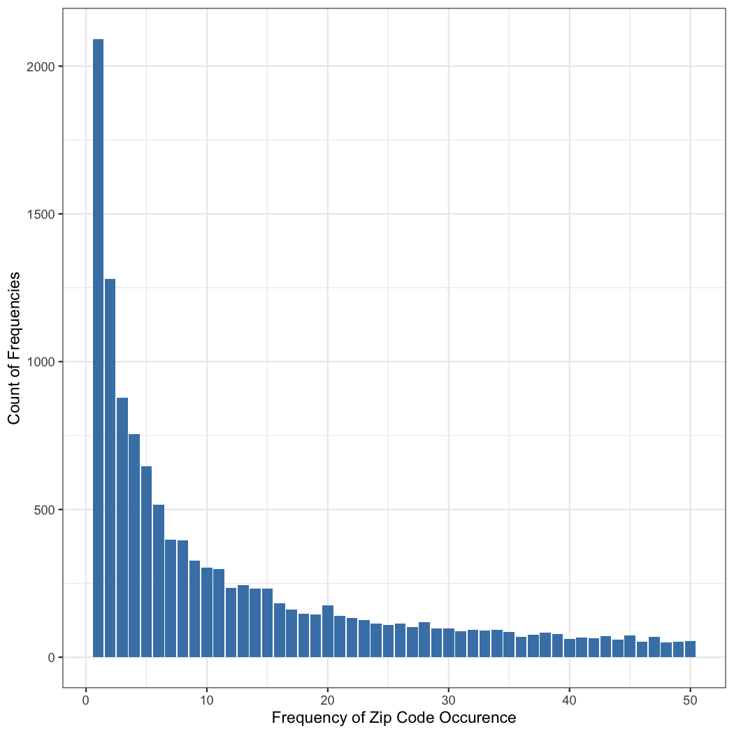
Figure 1 illustrates the frequency table of the zip codes in our data. On the x-axis is the frequency with which a zip code appears in the data, and on the y-axis is the count of zip codes that occurred with a given frequency. For instance, among the least popular zip codes, 5,031 zip codes were observed once, and 2,576 zip codes were observed twice. Among the most popular zip codes, 2 zip codes were observed 38 times each, 1 zip code was observed 40 times, and 1 zip code was observed 46 times. In total, 18,468 zip codes were selected at least once. Thus, the data describe a power law in the frequency with which zip codes occur, as expected, given that the basis on which the zip codes were sampled—the population distribution across zip codes—also follows a power law. We simulate this data on the basis of a marketing research context and question but similar datasets are likely to emerge in a host of social science settings. For instance, in any data that is randomly sampled from the U.S. population and then binned to the zip code to provide anonymity, we would expect the emergence of zip codes in the data to follow the same process as in our simulation.
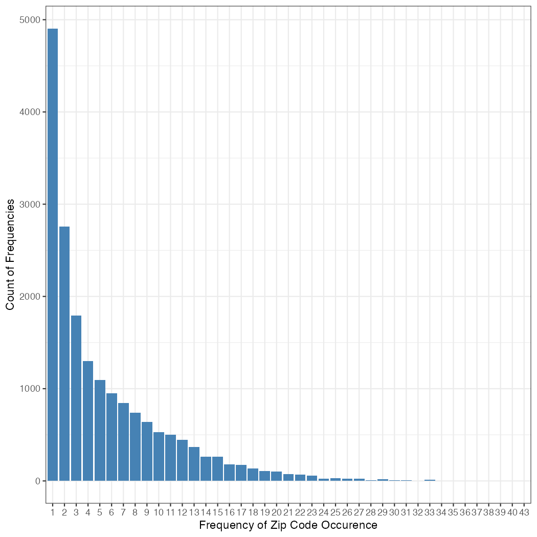
Note: The x-axis represents the frequency with which a zip code occurred in our simulation data. The y-axis shows the count of zip codes that occurred with each given frequency.
Our econometric model is formulated as follows:
where:
-
•
, , and represent the intercept, the coefficient on the price index, and the coefficients on the categorical variable (i.e., zip code fixed effects), respectively.
-
•
denotes the price.
-
•
is an indicator variable that equals one if consumer is located in zip code ; for simplicity, we use to denote a sum over all zip codes included in the model.
-
•
is the error term, assumed to follow a standard normal distribution.
In this specification, zip codes are treated according to their observed ambient space. Therefore, in data with 18,468 zip codes, it necessitates the inclusion of 18,468 category levels, resulting in a specification with 18,468 fixed effects. However, this space is underpinned by a manifold of latitude and longitude that determines the consumer’s location and, consequently, (i.e., the zip code). Thus, we further specify , where and are the coefficients on longitude and latitude on the manifold, respectively, and and represent the consumer’s longitude and latitude, respectively.
Our second simulation introduces elevation as a further dimension of the manifold, while adhering to earlier simulation specifications. We obtain the elevation of each zip code by extracting point elevations from the ‘AWS Terrain Tiles’, using the library ‘elevatr’ in R. As each latitude and longitude automatically defines elevation, we employ the same locations as in the first simulation but with the fixed effect now specified as , and , where is consumer ’s elevation.
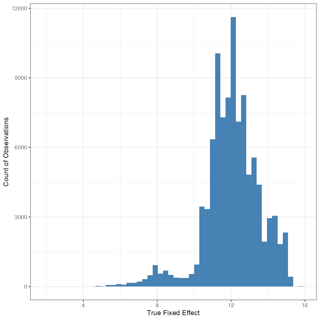
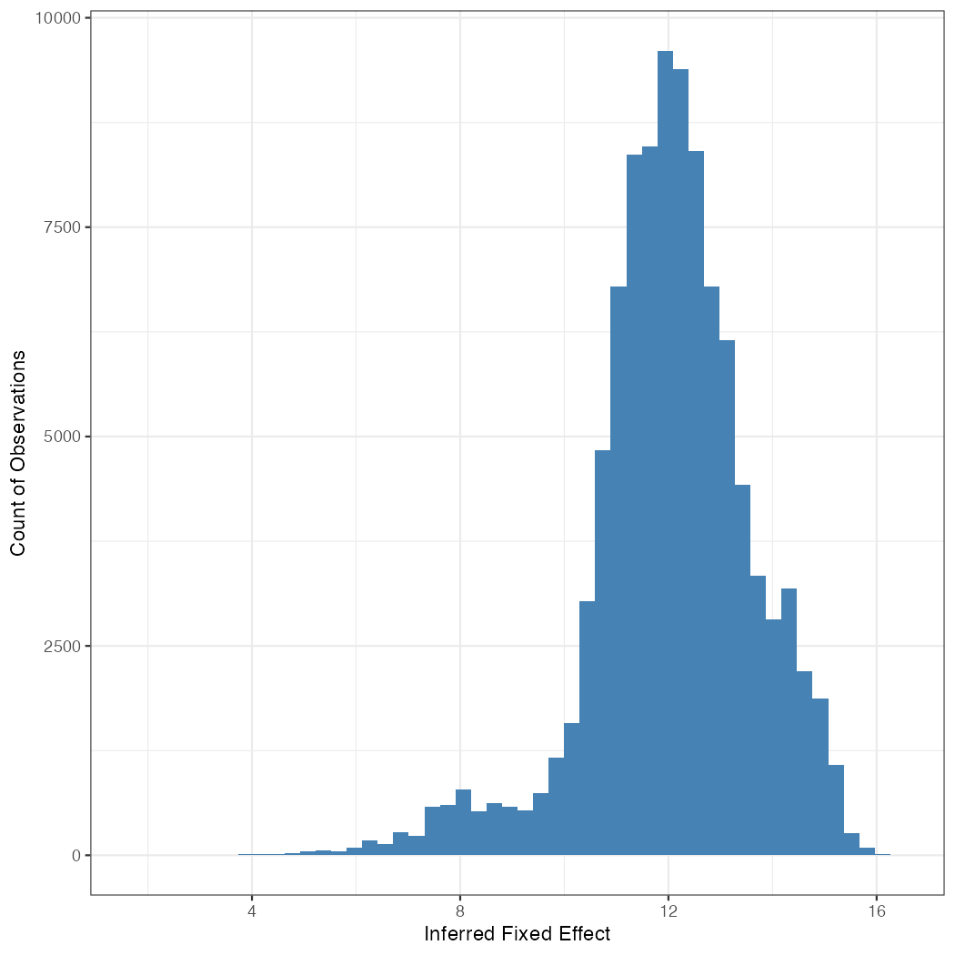
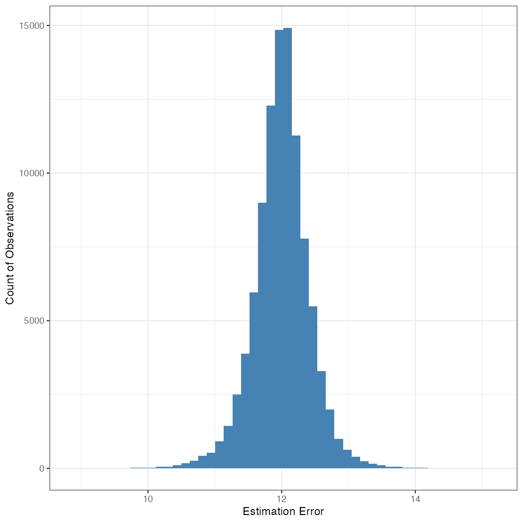
The key difference between the simulations is in the distribution of the fixed effects. In the first simulation, the fixed effect ranges from 0 in the northernmost zip codes to 4.895 in Key West, FL. The mean fixed effect is 2.305, and the standard deviation is 1. In the second simulation, the fixed effect ranges from 2.025 (in Buena Vista, CO) to 15.839 (in Oxnard, CA). The mean is 12.054, and the standard deviation is 1.518.
Results

Note: Estimation accuracy and precision in simulation 1 for the fixed effect coefficients.

Note: Estimation accuracy and precision in simulation 2 for the fixed effect coefficients. ECDF = Empirical cumulative distribution function.
Figure 2 and Figure 3 characterize estimation accuracy and precision in Simulations 1 and 2, respectively. They detail the true and inferred fixed effect coefficients using the standard regression estimator, as implemented by the ‘lm’ function in R, which automatically excludes category levels if the data are insufficient to provide a non-singular fit. In all simulations, the coefficient on price is estimated with great precision, as is to be expected in a simulation with 100,000 observations and where price is drawn from a uniform distribution.
Central to our research, and germane to our modeling advances, the coefficient on price is non-focal in our simulation and assumes the role of a nuisance variable. Instead, the analysis focuses on the coefficients on the zip codes where the estimation challenge is the high dimensionality of the categorical variable. In other cases, both population parameters and category-level (or group-specific) parameters may be crucial. We chose a simulation setup geared to illustrate the key benefits of our proposed method, but our model and innovations are applicable more broadly.
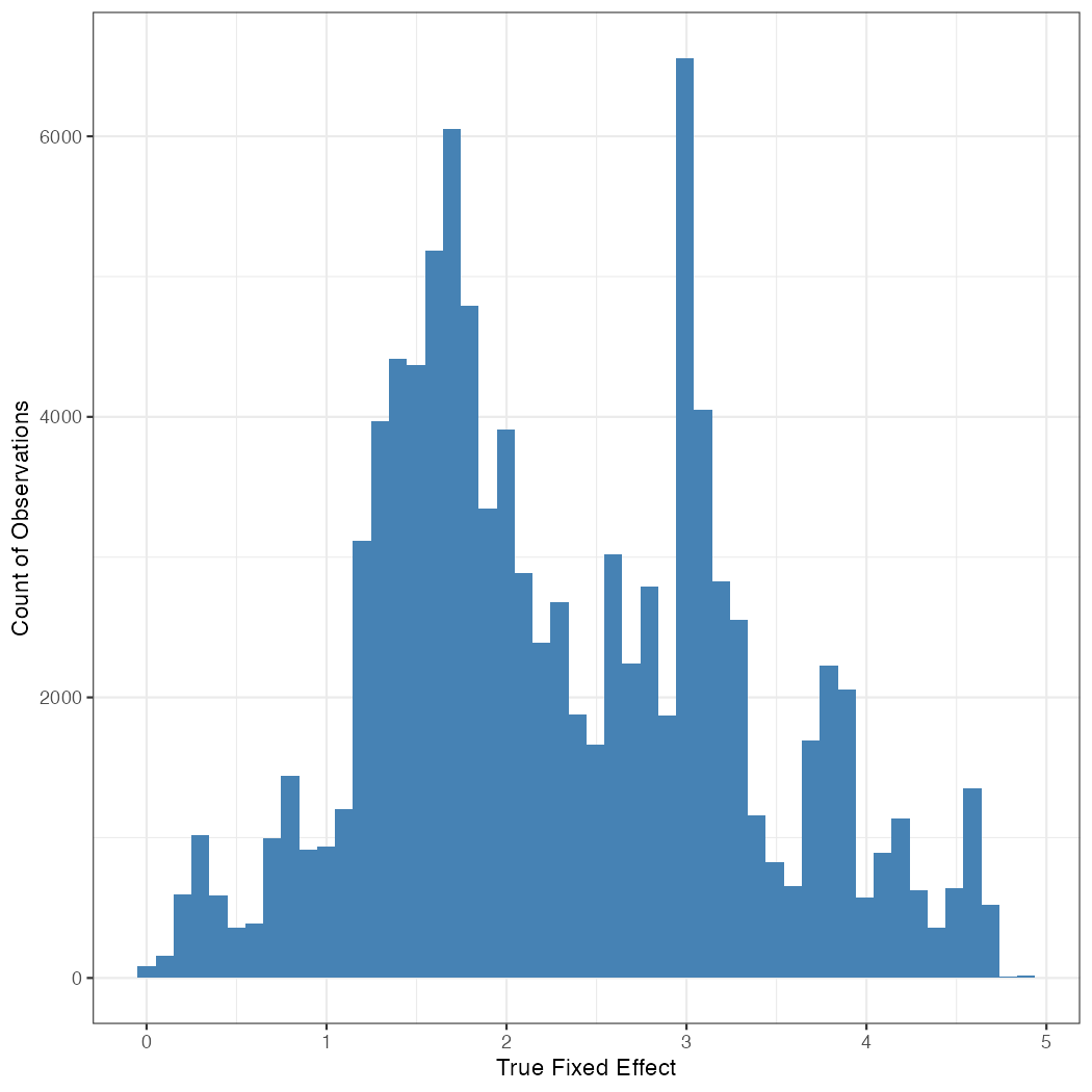
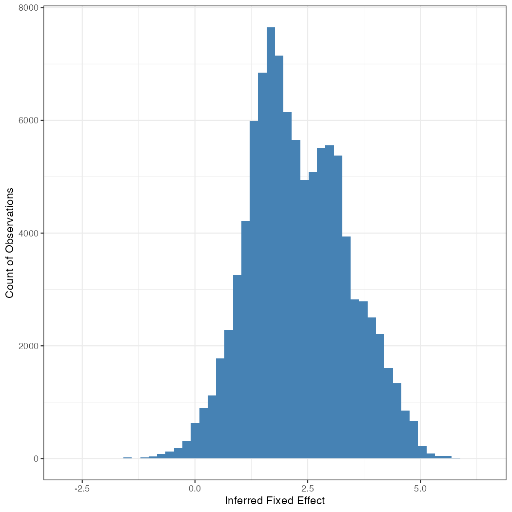
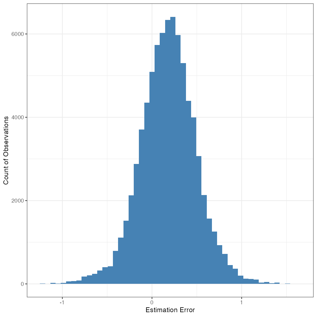
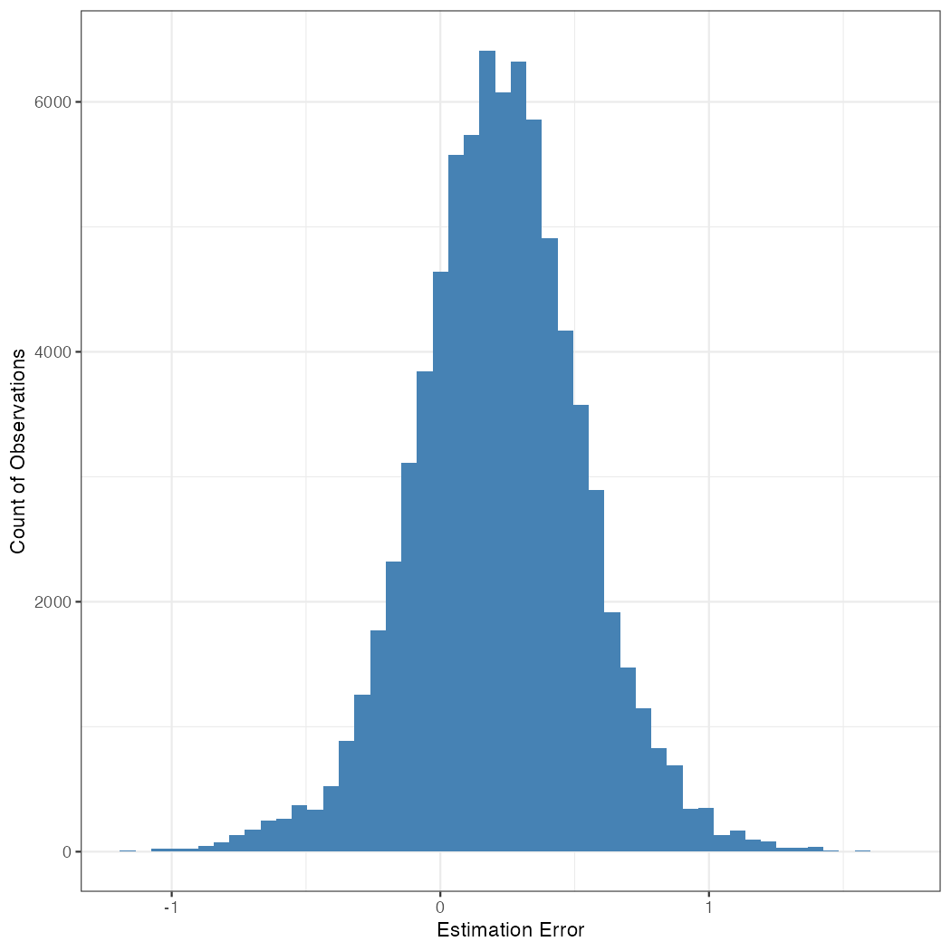
Subfigures 2(a) and 3(a) present a density of the true fixed effects, while subfigures 2(b) and 3(b) present a density of the inferred fixed effects. A visual comparison between these sets of subfigures reveals that the density of the inferred fixed effects does not resemble the density of the true fixed effects, despite the large sample size and relatively simple econometric specification. The difference between the density plots visually illustrates the issues we highlight in our analysis, whereby many estimates pertain to category levels that are estimated using only one or a few data points, leading to a distribution of fixed effect estimates that is vastly distinct from the original true fixed effects.
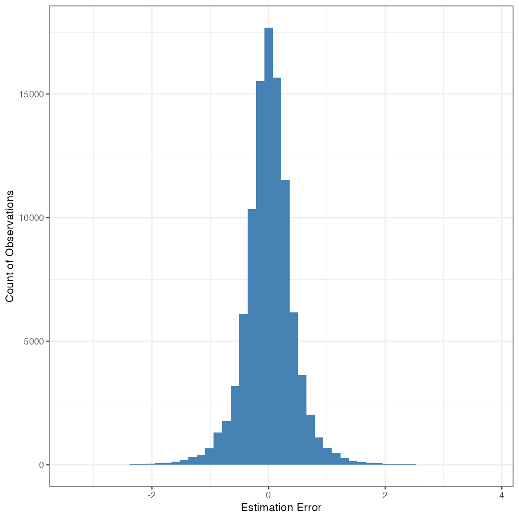
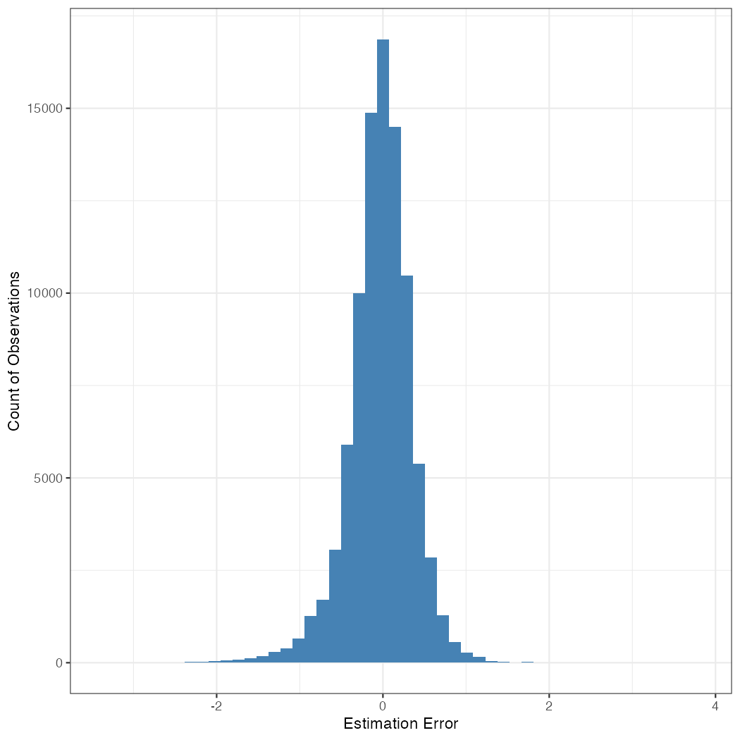
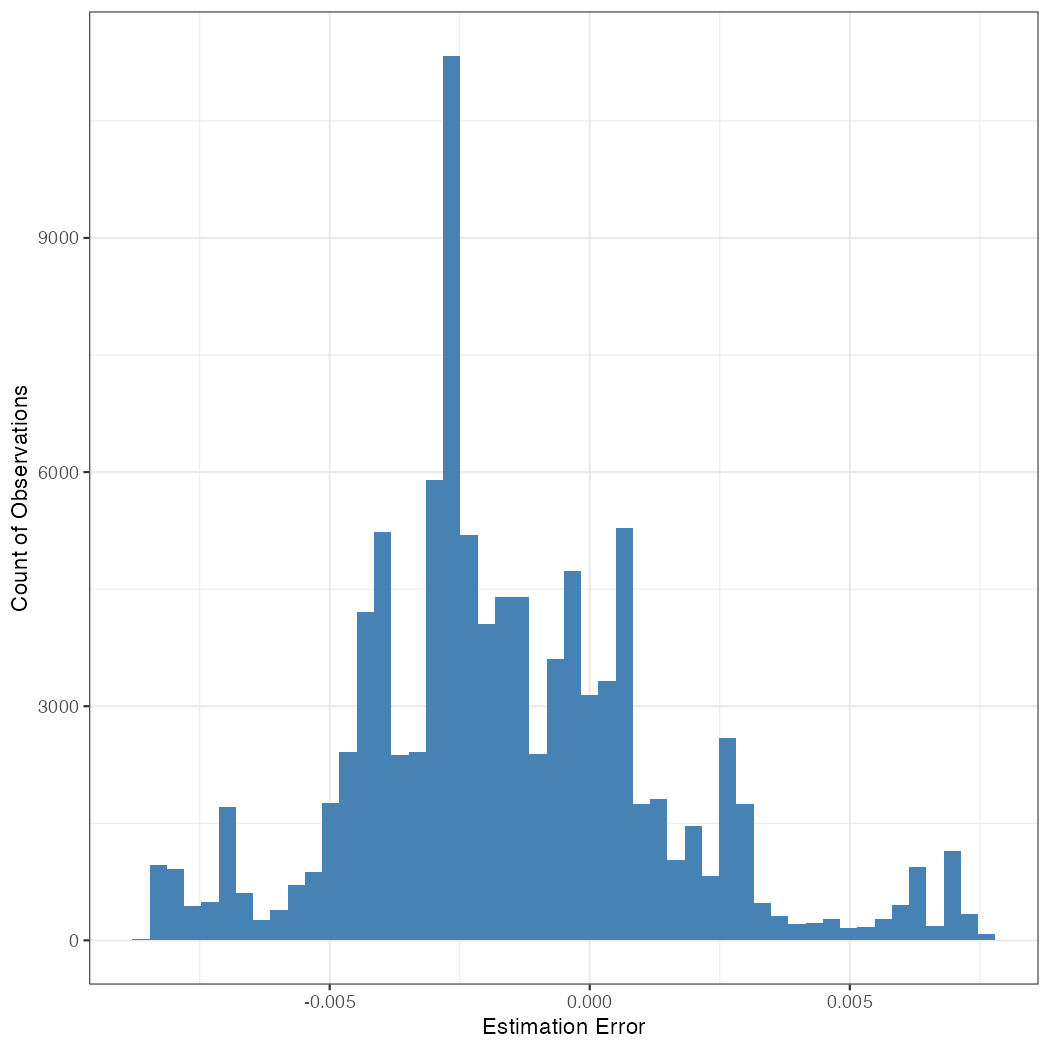
Subfigures 2(c) and 3(c) present histograms of the estimation error, which is the difference between the true fixed effect and the inferred fixed effect. While each coefficient estimate is imprecise, the expectation of the estimation error, taken over all fixed effects and observations, is 0; thus, the estimates are, on net, consistent. This is because in the multivariate regression, as long as there is some non-zero probability of a category level re-expressing, the fixed effect estimator is consistent. In our simulation, category levels (zip codes) are not dormant. Therefore, the estimates are consistent, and the sample average of estimation errors across coefficients is close to 0.
The distribution of the estimation errors is identical (to rounding error) in subfigures 2(c) and 3(c). This is because . Suppose for some , with and being the th observation of the dependent variable in the second and first simulations, respectively. It follows that , where is the regression estimator and is estimated precisely. Thus, only shifts the estimates—it has no effect on estimator precision.
This feature of the fixed effects model illustrates a key reason for our advocacy of PCA for dimensionality reduction. Namely, if the lower-dimensional embedding is a linear projection of the ambient space, as is the case with PCA, then the influence of each dimension of the manifold persists through the linear projection and a linear estimator such as the regression estimator. Consequently, each included or excluded dimension in the lower-dimensionality embedding has the clear and unambiguous meaning of contributing a projection of the fixed effect to its estimation. The inclusion of superfluous dimensions leads to more estimated null effects, greater data demands, and reduced precision while preserving consistency, whereas the exclusion of critical dimensions leads to biased estimates. For instance, projecting the fixed effects in simulation 2 on the manifold in simulation 1 would yield biased estimates due to the missing dimension (elevation).
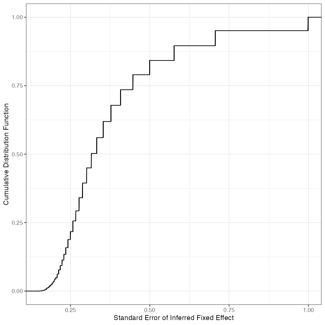
Subfigures 2(d) and 3(d) present the empirical cumulative distribution function (ECDF) of the precision (i.e., the standard errors) of the estimators. Here, we find variation in the extent of precision, with the visual analog of a step function where each step corresponds to a category level that found more expression in the data. Mirroring the symmetry of subfigures 2(c) and 3(c), subfigures 2(d) and 3(d) are also indistinguishable.
If all estimators converge, then the mean of the square of the standard errors of the fixed effects should converge to the variance of the inferred fixed effects around their true mean . The observed variance of the inferred fixed effects is 0.179 in our sample, whereas the expected precision (i.e., the average of the squared standard errors) is 0.184. This deviation is statistically significant as the standard error of the mean is 0.00216, yielding a t-statistic of 2.23.
This distinction occurs because the model overfits in-sample. For instance, the zipcode ‘01010’ is expressed only once in the data. Its inferred fixed effect is computed as where is the corresponding observation; the fixed effect is estimated using exactly one observation. It follows then that the estimator is unable to ascertain its own precision as the residual is 0. This implication of extreme sparsity is typical in power-law distributed category levels.
Note: Estimation accuracy and precision in simulation 1 for the fixed effect coefficients.

Note: Estimation accuracy and precision in simulation 2 for the fixed effect coefficients.
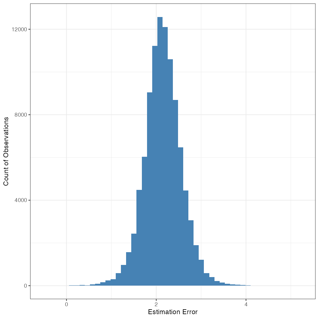
Figure 4 and Figure 5 characterize estimation errors from alternative approaches–the former presenting results from simulation 1 and the latter from simulation 2. Subfigures 4(a) and 5(a) present estimation errors corresponding to ‘significant’ estimates–which are coefficients that when tested against the null hypothesis yield a significant result. In these subfigures, we consider the classic and typical null hypothesis of the category level having no effect (the true coefficient is 0) as in practice, the true coefficient is not known and the estimated coefficients are statistically compared to 0. It is then typical to report and explain the significant coefficients as in those cases, the evidence supports a nonzero effect of the category level.
We find that 14,288 fixed effect coefficients (out of 18,468 total estimated fixed coefficients) are significant at the 5% level in simulation 1 and 18,467 fixed effect coefficients are significant in simulation 2; only one coefficient is nonsignificant in simulation 2. This illustrates a key concern in this strategy whereby the probability of a coefficient being significant is the composite of estimation precision and effect size. Thus, in this strategy, while the reporting strategy does not bias estimates as each estimate is still derived from the inclusion of all categorical levels, the reported levels are biased towards the confluence of lower estimation uncertainty and higher effective sample size. Thus, for example, Figure 3(a) is virtually indistinguishable from Figure 5(a) as the histogram differs on only 1 point estimate–the single coefficient that is nonsignificant at the 5% level.
Subfigures 4(b) and 5(b), we present estimates from an estimator where infrequent category levels are merged for inclusion with the intercept, and the model is estimated using the ‘lm’ function in R. In this case, we observe the mean of the fixed effects is no longer zero due to a change in the meaning of the fixed effects. The process does tamp down the variance. Thus, we observe lowered variance at the expense of bias.
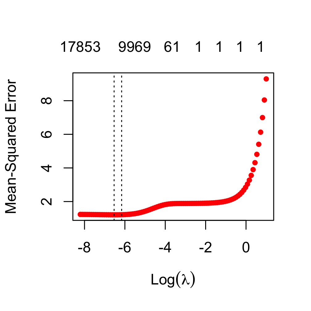
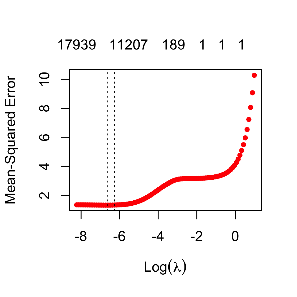
Subfigures 4(c) and 4(d), as well as 5(c) and 5(d), relate to the use of LASSO, estimated with the ‘glmnet’ function from the ‘glmnet’ package in R, where the hyperparameter is selected through cross-validation using ‘cv.glmnet’. The first two subfigures pertain to simulation 1, and the latter two to simulation 2; the first and third subfigures describe model performance for various values of . The second and fourth subfigures depict the estimation errors when ‘lambda.1se’, which is the largest value of such that the error is within 1 standard deviation of the cross-validated minimum, is chosen.
Cross-validated LASSO suggests the inclusion of many categorical variable levels. In simulation 1, the minimum cross-validated error is achieved when lambda is 0.001453, and 15,242 levels are included. The largest value of such that the error is within 1 standard deviation of the cross-validated errors is 0.002109, where 13,784 levels are included. In simulation 2, the corresponding numbers are 0.001299 and 16,002 for the minimum error, and 0.001884 and 14,920 levels for error within 1 standard deviation of the minimum. As a reminder, the data includes 18,468 levels, of which 5,031 were only observed once. Thus, the use of LASSO does not lead to the exclusion of variables that are estimated using only 1 observation—in many cases, the estimation of a fixed effect even from a single observation is critical to cross-validated model fit, as in its absence, the average of the excluded fixed effects is a poor substitute for the excluded category level.
Critically, despite the inclusion of the majority of the categorical variables in an effort to reduce the variance of estimates, we observe both bias and considerable imprecision in subfigures 4(d) and 5(d) that depict the estimation errors when ‘lambda.1se’, which is the largest value of such that the error is within 1 standard deviation of the cross-validated minimum, is chosen. This illustrates the dilemma such data presents to the researcher: including all categorical levels leads to imprecision, but merging or dropping levels through the use of an ad-hoc strategy or through principled discovery using cross-validated LASSO is also ineffective at mitigating instability.
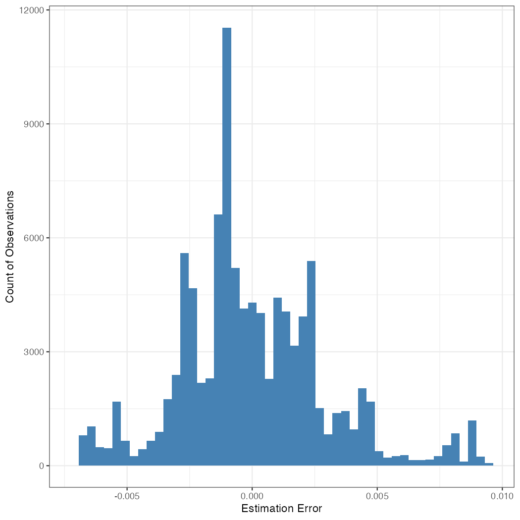
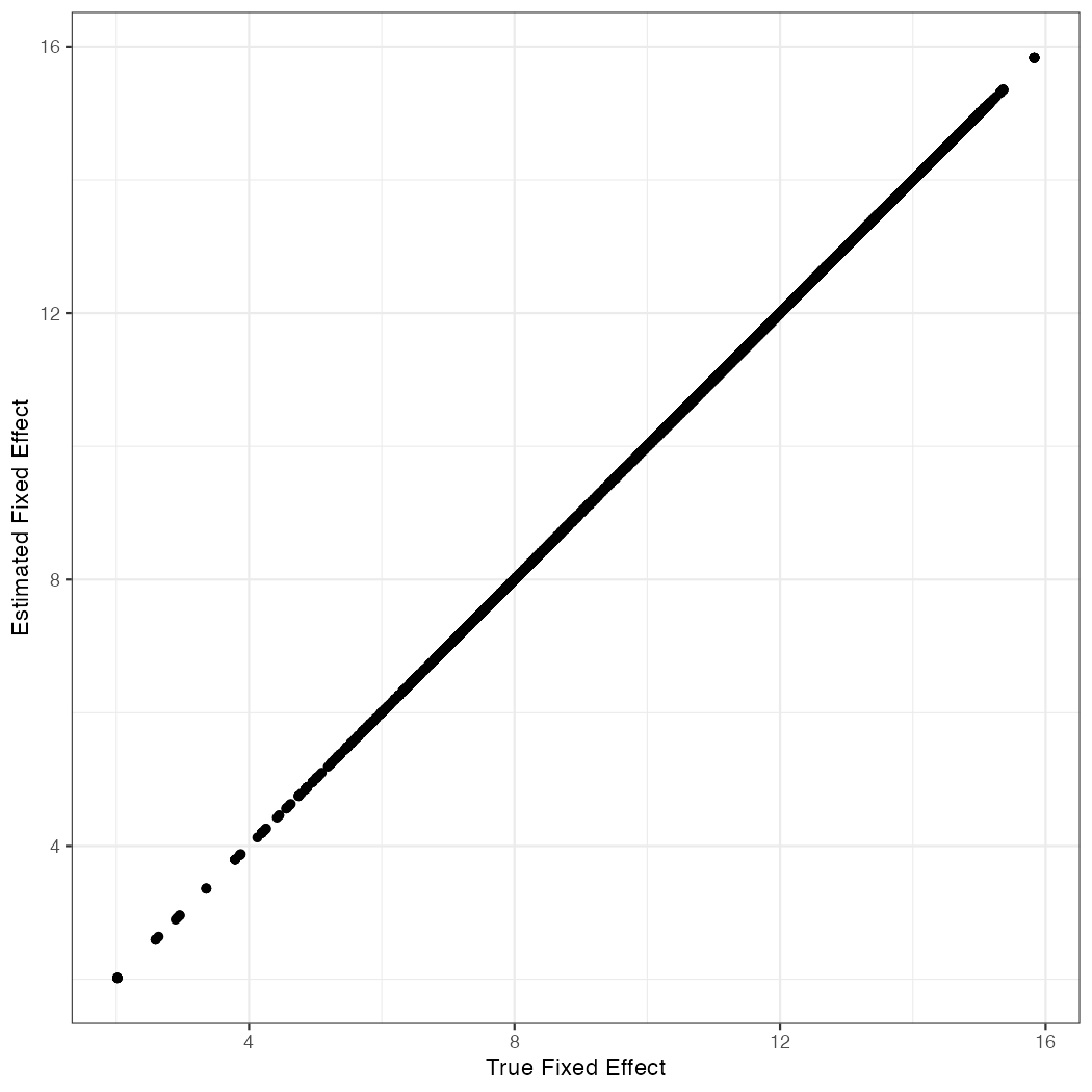
Note: Estimation accuracy and precision using our proposed estimator for the fixed effect coefficients.
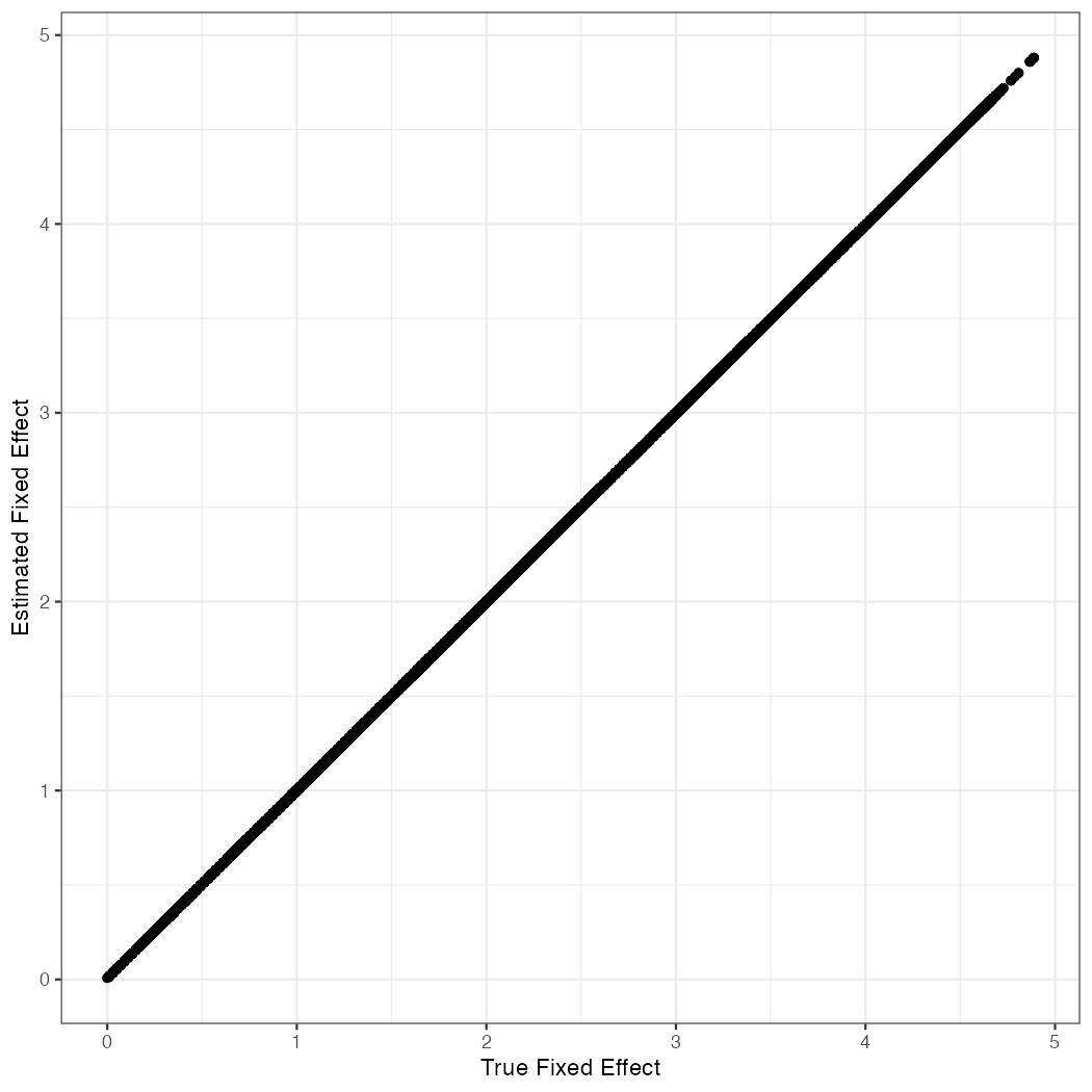
Figure 6 presents estimates from our proposed approach in both simulations. The figure comprises four subfigures of which subfigures 6(a) and 6(b) address simulation 1, and subfigures 6(c) and 6(d) address simulation 2. The first and third subfigures are histograms of the estimation error and the second and fourth subfigures plot the estimate against the true coefficient. In all cases, our proposed approach yields analysis that is more accurate and more precise as it relates the fixed effect to its determinants. The imposed structure provides the model with both the statistical scaffolding needed to ensure precise estimation, and a means to capture the variation in the fixed effects.
Application: Direct-to-Consumer Sales
We analyze data from an online apparel provider that was a pioneer in direct-to-consumer sales. Our data covers a period from the early days of internet retailing when the firm was the market leader, facing little to no competition from similar firms. Therefore, our data uniquely tracks the evolution of both the firm and the industry during this pivotal period. Although the identity of the data-providing firm cannot be disclosed, it is noteworthy that the firm launched waves of new apparel products sold exclusively to consumers through their platform. For the purposes of our analysis, we operate under the assumption that the firm primarily sold summer apparel, which serves as an illustrative example of their product category. Given that the firm was founded on the East Coast and initially found success in both the East Coast and Midwest regions, we anticipate, contrary to our simulations, observing the influence of longitude on fixed effects.
Our overarching goal is to conduct demand analysis, aiming to measure demand at the zip code level. Specificity in such analyses is crucial as it informs managerial decisions, such as the locations for physical stores. In this particular case, the firm initially lacked a brick-and-mortar presence but later expanded offline. While specific details about store openings are confidential and not directly traceable in this study to protect the company’s identity, we can confirm that the selected cities for physical stores align with the ‘hot spots’ identified in our data—areas showing the highest demand for the company’s products.
Data
The data pertains to orders from the contiguous United States. Figure 7 plots a heatmap of order frequency by zip code on a map of the United States, where a darker color corresponds to higher order volume for a zip code. We see that the order volume is anchored in a few major cities such as Seattle, San Francisco, Los Angeles, Chicago, New York, and Washington DC, but otherwise dispersed throughout the United States.
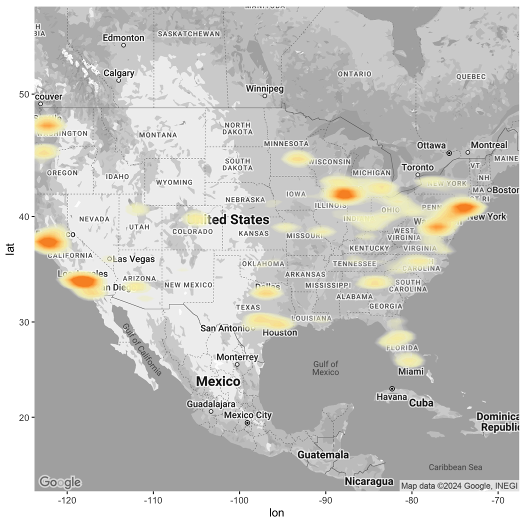
Note: Color and opacity represent order volume.
We present the following figures to illustrate the key modeling challenge. Figure 8 plots the number of unique zip codes for every 1,000 observations in the data, starting from the inception of the firm and ordered according to when the observations occurred. This figure demonstrates the number of unique zip codes that the firm might expect to encounter in a data sample of a specified size if the data were collected from the beginning of the firm’s operation. Specifically, our complete dataset comprises 1,985,365 observations. Therefore, the figure presents the number of unique zip codes for nearly 2,000 data samples, illustrating the growth in the number of zip codes, which is central to the data challenge that we seek to address in this paper.
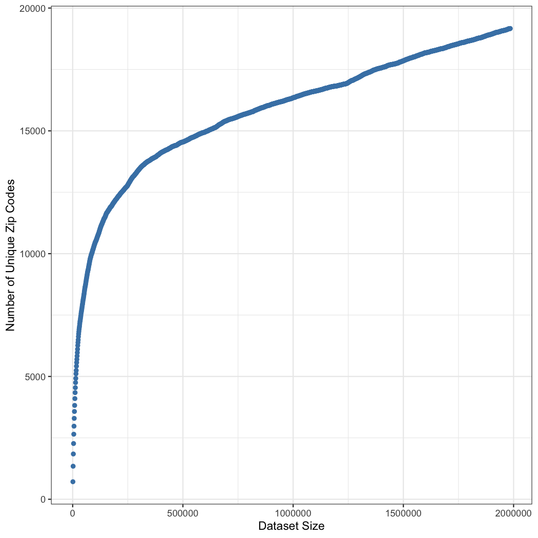
Note: On the y-axis is the number of unique zip codes. On the x-axis is the sample size.
We observe a steep increase in the number of unique zip codes in the data during the initial quarter of the data, covering the first 500,000 observations. While the rate at which additional zip codes are observed in the data diminishes with the accrual of data, throughout our entire dataset of almost 2 million observations, we find that the number of zip codes does not level off and continues to increase with the data. Thus, in a classical model where zip codes are introduced in the specification as a categorical variable, the number of levels would remain a function of sample data points for the duration of our dataset.
Analogous to Figure 1 in our simulation data, Figure 9 illustrates the frequency table of the zip codes in our field data. The figure is split into two subfigures for improved presentation: the top panel (subfigure 9(a)) presents the count of frequencies on the y-axis and the frequency on the x-axis for the least common zip codes; the bottom panel (subfigure 9(b)) presents similar statistics with the axes reversed for all frequencies of all zip codes.
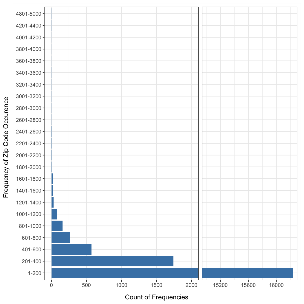
Note: Frequency with which a zip code occurred in the field data and the count of zip codes that occurred with a given frequency.
The zip codes (the focal independent variable in our study) exhibit a power-law distribution, whereby a few zip codes have many observations (the most frequent zip code in our data—Chicago, IL, 60657—has 5,758 observations), and 3,372 zip codes have either one or two corresponding observations. In total, the data pertains to 19,170 zip codes, which represents only about two-thirds of the zip codes in the United States. Therefore, the sparsity concerns we highlight are likely to persist even if a much larger data sample were collected.
Including 20,000 zip codes in an econometric model, and estimating on 2 million data points, would likely be impractical for most researchers. For instance, with 20,000 indicator variables and 2 million observations, the design matrix would require approximately 320 GB of memory just for storage—estimation would necessitate even more memory. These data demands would scale supralinearly with the inclusion of more data as in addition to adding rows to the design matrix, the addition of data is likely to lead to the addition of indicator variables through the addition of novel category levels (i.e., zip codes).
Therefore, we constructed a random sample of 100,000 observations from the complete dataset for estimation purposes. Figure 10 presents the frequency table of zip codes in this data subsample. As expected, a power-law distribution of zip codes is observed, with 5,272 zip codes appearing two or fewer times in the subsample and one zip code appearing 269 times. It’s noteworthy that the sparsity patterns in our field data subsample are less pronounced than those observed in our simulations. Specifically, in our simulations, 18,468 zip codes were selected at least once, whereas in our field data subsample, 11,411 zip codes were selected at least once. This discrepancy suggests that the dispersion of orders across zip codes in the field data is not entirely random. Likely, the firm’s products are more popular in certain zip codes, leading to repeat orders. Nonetheless, the field data still illustrates the power law distribution that is central to the modeling challenge addressed in our paper.
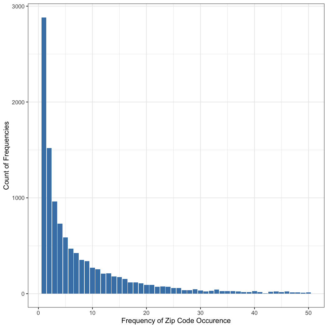
Note: The x-axis represents the frequency with which a zip code occurred in our field data. The y-axis shows the count of zip codes that occurred with each given frequency.
Model Specification
Our dependent variable is revenue per order (inclusive of any shipping and handling charges). As a focal covariate, we consider the use of a coupon, a common practice in internet retailing that significantly lowers the order value and drives order growth. We incorporate fixed effects for zip codes, to delineate the firm’s geographic expansion and include dummy variables for both month and year to account for seasonality and to capture the growth in the firm’s product portfolio and its appeal over time. Thus, we specify the model as follows:
where:
-
•
is revenue inclusive of shipping and handling. , , , , and denote the intercept, the coefficient on the coupon, and the fixed effects for zip code, month of purchase, and year of purchase, respectively. represents the time index, and signifies the consumer index.
-
•
is an indicator variable that equals one if consumer utilized a coupon at time .
-
•
is an indicator variable that equals one if consumer resides in zip code .
-
•
and are indicator variables for the month and year of purchase, respectively, equaling one if corresponds to month and year .
-
•
is the error term, assumed to have a mean of zero.
To predict the fixed effects associated with each zip code, we consider the latitude, longitude, and elevation of each zip code. Given the anonymization of consumer addresses to the zip code level in our dataset, we utilize the centroid of each zip code to derive these auxiliary variables.
We introduce two forms of additional information to enhance our model’s predictive accuracy for zip code fixed effects. First, we incorporate the encoding from OpenAI’s ‘text-embedding-3-large’ model of each zip code’s name and address (e.g., ‘10001 New York, NY’). This approach recognizes that distinct zip codes, even those at similar elevations, can exhibit cultural differences that may influence demand. For instance, demand for summer apparel in Berkeley, CA, might differ from that in San Francisco, CA, despite their geographical proximity. Given the extensive data features provided by both structured data points (latitude, longitude, and altitude) and the LLM capture of the town/city name, direct inclusion of the LLM encoding in the statistical model is impractical. Therefore, we employ PCA for rank reduction, allowing us to retain essential descriptors while excluding irrelevant data features related to inter-zip code differences.
Second, we utilize a series of variables describing the geographical and socio-economic characteristics of each zip code as additional predictors of the fixed effect. Here, we replace the unstructured LLM encoding based on the zip code and associated address with structured information such as median home value, which also reflects systematic differences among zip codes. To assess the extent of overlap in their informative content and examine the extent to which these variables provide complementary insights into the fixed effects associated with each zip code, we specify a model incorporating both structured and unstructured information.
Table 1 presents key descriptive statistics of the data for the mainland states of the United States; we exclude observations related to international sales and those to Hawaii and Alaska to maintain a contiguous definition of zip codes.
| Variable | N | Mean | St. Dev. | Min | Max |
| Revenue Per Order | 1,985,365 | 35.966 | 40.899 | 0.010 | 14,402.380 |
| Coupon | 1,985,365 | 0.084 | 0.278 | 0 | 1 |
| Latitude | 1,985,365 | 37.895 | 4.971 | 24.600 | 48.990 |
| Longitude | 1,985,365 | 96.830 | 17.413 | 124.500 | 71.940 |
| Elevation | 1,985,365 | 250.328 | 374.123 | 858 | 3,870 |
| Housing Units | 1,985,365 | 14,263.680 | 7,439.505 | 16 | 47,617 |
| Land Area | 1,985,365 | 35.693 | 91.585 | 0.020 | 3,911.400 |
| Median Home Value | 1,985,365 | 328,507.200 | 223,369.500 | 10,200 | 1,000,001 |
| Median Household Income | 1,985,365 | 66,062.560 | 26,331.730 | 2,499 | 250,001 |
| Occupied Housing Units | 1,985,365 | 13,118.470 | 6,857.844 | 12 | 44,432 |
| Population Density | 1,985,365 | 6,703.375 | 13,711.620 | 0 | 143,683 |
| Water Area | 1,985,365 | 1.040 | 4.171 | 0.000 | 255.390 |
Results
Initially, we present findings from regressions conducted on our random subsample of 100,000 observations across four distinct scenarios, where the zip code variable is specified at different levels of aggregation. This approach leverages the hierarchical nature of zip codes, with the first digit representing a broad geographic grouping of states, two digits representing a sectional center facility (SCF, a major mail processing center within a region), three digits designating a more specific area within the SCF, and the full zip code pinpointing a specific delivery area, such as a neighborhood or a group of streets. While this hierarchy may not always effectively capture consumption pattern differences—for example, Buffalo, NY, may have more distinct consumption patterns from Manhattan, NY, than Princeton, NJ, a city much closer to Manhattan—it offers a structured approach to the inclusion of categorical variables. This approach is particularly useful in practice when faced with the challenges of managing many unique levels and data that might otherwise overwhelm the model.
Table 2 presents our findings. Columns 1, 2, 3, and 4 present results from the inclusion of 1-digit, 2-digit, 3-digit, and 5-digit zip code levels, respectively. The first two models are relatively stable, with 8 and 89 fixed effects estimated from 100,000 observations. The third model is also somewhat stable, as more than 100 observations correspond to each zip code on average. However, in 14 cases, only 1 observation supports inference, and in 13 cases, only 2 observations support inference. Thus, in the third model, the effects of category sparsity begin to emerge, even though the data is sufficiently large to support the estimation of many of the included zip code fixed effects.
The fourth model is saturated, as the data includes 11,411 unique zip codes. For instance, in 2,961 cases, inference is supported by 1 observation; in 1,450 cases, inference is supported by 2 observations; and in 986 cases, inference is supported by 3 observations. Consequently, the models’ adjusted R-squared, which is 0.028 and 0.029 for the first two models that are not saturated, increases to 0.032 for the third model that is slightly saturated and 0.151 for the fourth model, which is highly saturated. This saturation implies that the residuals corresponding to observations where the categories are sparse (i.e., only one or a few observations correspond to the category) are fit with little to no error. In these cases, the fixed effect suffices to perfectly or almost perfectly explain the observations, improving the fit statistic drastically. Our knowledge that the first 2 models are relatively less saturated suggests that an R-squared of about 0.029 is a more accurate reflection of the extent to which zip codes explain the variance in order values across geography.
| Dependent variable: Revenue Per Order | ||||
| (1) | (2) | (3) | (4) | |
| Coupon | 20.239∗∗∗ | 20.215∗∗∗ | 20.292∗∗∗ | 20.537∗∗∗ |
| Constant | 37.971∗∗∗ | 41.020∗∗∗ | 41.143∗∗∗ | 46.224∗∗∗ |
| # 1-Digit Zip Code | 9 | 0 | 0 | 0 |
| # 2-Digit Zip Code | 0 | 90 | 0 | 0 |
| # 3-Digit Zip Code | 0 | 0 | 787 | 0 |
| # 5-Digit Zip Code | 0 | 0 | 0 | 11411 |
| Observations | 100,000 | 100,000 | 100,000 | 100,000 |
| R2 | 0.028 | 0.030 | 0.039 | 0.151 |
| Adjusted R2 | 0.028 | 0.029 | 0.032 | 0.043 |
| Residual Std. Error | 33.980 | 33.956 | 33.907 | 33.715 |
| (df = 99990) | (df = 99909) | (df = 99217) | (df = 88726) | |
| F Statistic | 316.956∗∗∗ | 34.233∗∗∗ | 5.210∗∗∗ | 1.396∗∗∗ |
| (df = 9; 99990) | (df = 90; 99909) | (df = 782; 99217) | (df = 11273; 88726) | |
| Note: | ∗p0.1; ∗∗p0.05; ∗∗∗p0.01 | |||
We used a subsample in this analysis due to computational stability and cost concerns. Running a regression with 100,000 observations and five-digit zip code fixed effects using ‘lm’ in R took approximately 4 hours on a multicore state-of-the-art workstation (Apple Studio M2 Ultra). Given that computational costs in regression analysis tend to scale cubically, we estimate that even if the workstation had access to sufficient working memory, the computational time would be cost-prohibitive, potentially requiring upwards of 32,000 hours for our entire dataset.
Moreover, while routines have been developed for fast fixed effect estimation, such as iteratively reweighted least squares (Hinz et al. 2019), these methods rely on distributional assumptions about the link function. In contrast, identification in the regression model only requires specifying the orthogonality of the residuals with respect to the regressors and a convergence of the second moments to a positive semi-definite matrix. Although a clever pairing of optimization methodology and specific econometric models may yield a computationally stable estimation routine in certain cases, estimation in the general case remains computationally challenging. This computational hurdle, in addition to the statistical concerns raised by the saturation of degrees of freedom due to the inclusion of many fixed effect parameters (as seen in Models 3 and 4), further justifies the development of our model.
Table 3 summarizes estimates when fixed effects are projected to a lower dimensional space. We specify four models. The first model includes only the latitude, longitude, and elevation of the zip code. This model corresponds to our simulations and represents a baseline explanation of the variation in demand across zip codes. Model 2 includes a set of key economic descriptors that track cultural (e.g. population density tracks rural vs. urban), economic (e.g., household), geographic (e.g. land area), and social (e.g., housing density) factors that may explain differences in demand.
| Dependent variable: Revenue Per Order | ||||
| (1) | (2) | (3) | (4) | |
| Coupon | 21.431∗∗∗ | 21.408∗∗∗ | 21.432∗∗∗ | 21.404∗∗∗ |
| Latitude | 0.045∗∗∗ | 0.054∗∗∗ | 0.155∗∗∗ | |
| Longitude | 0.046∗∗∗ | 0.027∗∗∗ | 0.085∗∗∗ | |
| Elevation | 0.001∗∗∗ | 0.0001∗ | 0.0001 | |
| Home Value | 0.00001∗∗∗ | 0.00000∗∗∗ | ||
| Household Income | 0.00002∗∗∗ | 0.00002∗∗∗ | ||
| Housing Units (HU) | 0.0005∗∗∗ | 0.0004∗∗∗ | ||
| Land Area | 0.001∗∗∗ | 0.002∗∗∗ | ||
| Occupied HU | 0.001∗∗∗ | 0.0005∗∗∗ | ||
| Population Density | 0.00005∗∗∗ | 0.00002∗∗∗ | ||
| Water | 0.081∗∗∗ | 0.080∗∗∗ | ||
| Constant | 35.246∗∗∗ | 36.460∗∗∗ | 36.103∗∗∗ | 30.817∗∗∗ |
| OpenAI Encoding | No | No | Yes | Yes |
| Observations | 1,985,365 | 1,985,365 | 1,985,365 | 1,985,365 |
| R2 | 0.022 | 0.023 | 0.023 | 0.024 |
| Adjusted R2 | 0.022 | 0.023 | 0.023 | 0.024 |
| Residual Std. Error | 40.456 | 40.428 | 40.418 | 40.410 |
| (df = 1985360) | (df = 1985353) | (df = 1985331) | (df = 1985321) | |
| F Statistic | 10,947.300∗∗∗ | 4,231.140∗∗∗ | 1,441.538∗∗∗ | 1,126.590∗∗∗ |
| (df = 4; 1985360) | (df = 11; 1985353) | (df = 33; 1985331) | (df = 43; 1985321) | |
| Note: | ∗p0.1; ∗∗p0.05; ∗∗∗p0.01 | |||
Models 3 and 4 include 32-dimensional encoded representations formed by employing ‘text-embedding-3-large’ on each zip code’s name and address (e.g., ‘10001 New York, NY’). We chose to use the first 32 dimensions after empirical testing, as the inclusion of more singular vectors neither substantially improved model fit nor changed our substantive results. Our results show that the inclusion of the OpenAI encoding led to model results that are substantively similar to the inclusion of the structured data describing geographies, potentially due to representation being a lower-dimensional capture of the address of each zip code and therefore an encoding of the unique cultural, economic, geographic, and social factors of each zip code. Broadly, thus, we show that the LLM encoding of unstructured data describing the zip codes can yield similarly useful results as detailed structured data describing the zip codes—the implicit knowledge graph stored in the LLM’s weights and its expression in the embedding suffices to describe demand in our application.
Why might a model with the inclusion of 1-digit zip code fixed effects have a slightly higher R-squared than the model with geographic and other variables? A detailed look at the regression with 1-digit zip codes reveals that only four zip code fixed effects corresponding to a first digit of 2 (DC, MD, NC, SC, VA, and WV), 3 (AL, FL, GA, MS, and TN), 4 (IN, KY, MI, and OH), and 5 (IA, MN, MT, ND, SD, and WI) are significant in the regression. The intercept in the regression is $38.61, and the coefficient on the coupon is -$19.54. In contrast, the zip codes starting with 2, 3, 4, and 5 have coefficients of -$2.50, -$1.47, -$3.39, and -$1.73, respectively, which is on the order of 10% or less of the intercept and 5% or less of the coupon. Thus, what we find is that demand across geographies was relatively homogenous for this firm, with limited variation explained by the location of the customer—a conclusion that stands across the two stable models using zip code fixed effects and the projection of the fixed effects to structured and unstructured data covariates. This is perhaps not surprising, as this firm was born on the internet, targeted relatively young consumers, and its products were only retailed direct to consumer. Therefore, it follows that there was limited variation in revenue per order across different geographies, with most of the variation explained by longitude (the extent to which the firm was able to diffuse from the east to the west) and latitude (the extent to which its products could be used around the year, including in winter).
Figure 11 presents histograms of the fixed effect estimates and standard errors from Model 4 in Table 3. We see that the estimates range from about 1 to 10, suggesting a difference of about $10 in spend per order across geographies (estimation error is centered around $1 with relatively low dispersion). This suggests that smoothing out the estimates of spend by employing structured and unstructured descriptions of variations across zip codes yields a model that expresses greater geographic differences in mean spend. The standard errors mostly range from 1.25 to 1.5, with a mean of 1.374 and a standard deviation of 0.07. 99.22% of the estimates are significant against the null at a confidence level of 95%, indicating a robust capture of the fixed effects.
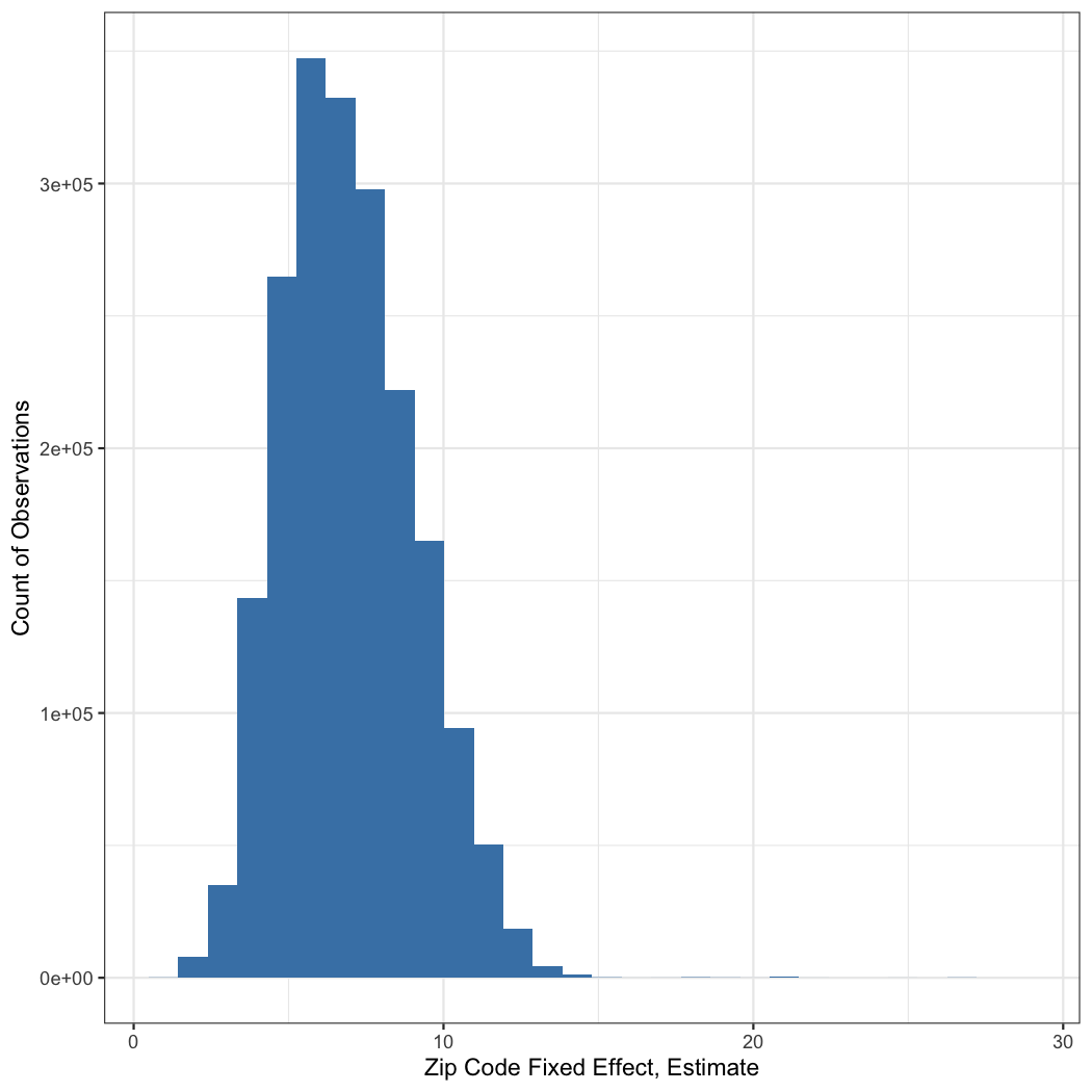
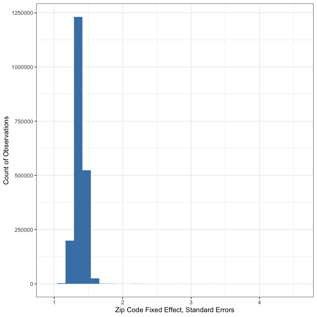
Figure 12 maps the inferred fixed effects in Model 4 to the location of the zip code in the United States. We find that revenue per order, accounting for couponing, varies drastically across the United States such that in high demand markets (see Figure 7) not only are more orders placed but also the revenue per order is higher than in lower demand markets. However, the effects are clearly not universal. For example, order volume from cities in the east coast of Florida (e.g. Miami, FL) is high. However, the estimated fixed effect and therefore the revenue per order is higher than other cities with comparable order volume, indicating that these cities are likely prime targets for offline expansion.
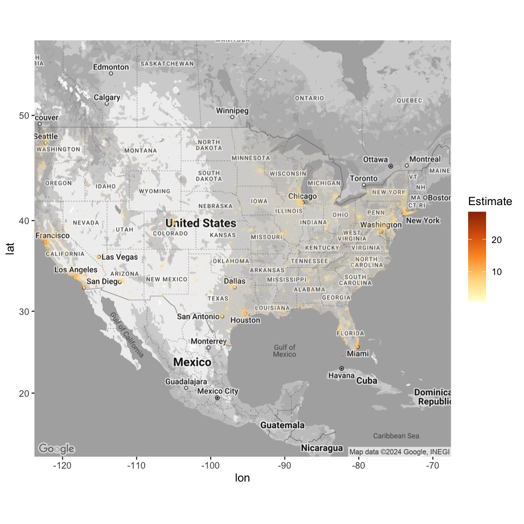
Note: Color and opacity represent fixed effect magnitude.
Conclusion
In this paper, we investigate the integration of categorical variables with a power-law distribution into causal econometric models. Our findings indicate that traditional regression estimators, affected by the sparse and unbounded nature of category levels, may not converge to accurate values, leading to both inaccurate and imprecise inferences. This issue arises from the violation of the Donsker conditions, essential assumptions for the asymptotic normality of estimators and the parametric complexity in econometric models. The lack of these conditions undermines the reliability of convergence guarantees.
Through numerical simulations, we reinforce these theoretical insights, showing that estimates from both the canonical estimator and those using widely accepted methodological practices—such as excluding or merging rare categories, or applying regularization techniques like LASSO for variable selection—yield inconsistent estimates. Moreover, this problem is exacerbated as models tend to overfit the data, complicating the reliability of in-sample and asymptotic fit statistics, making these issues difficult to detect and address.
To address this challenge, we propose a novel estimator that leverages knowledge of the underlying manifold from which the categorical variable’s expression in the ambient space is derived. In our empirical work, we position this within a spatial econometrics framework, where a categorical variable of zip code is distributed as sampled from a manifold of latitude, longitude, and elevation. We demonstrate that by using auxiliary information to describe the category levels—whether it be structured data on the levels or even unstructured data describing the levels as mapped using a large language model—we can infer category-level data features that form the scaffolding on which estimates can be derived. This auxiliary information on category levels enables our model to surpass the traditional inclusion of dummies in the canonical model, which is typically considered the efficient estimator. Unlike the canonical model, which involves a non-parametric capture of the fixed effects, our approach advocates for an explicit modeling of these effects.
Our method has broad applicability across various research fields and industry sectors where high-dimensional categorical data is prevalent. For example, in healthcare analytics, patient data often includes categorical variables such as diagnosis codes and treatment codes. Previous work has shown the potential of using deep learning to generate unsupervised patient embeddings from electronic health records (Choi et al. 2016, Miotto et al. 2016).
Extending our approach could involve using the LLM encoding of each diagnosis code or treatment code as a set of explanatory covariates for the fixed effect. This would transform the high-dimensionality non-parametric model, which might result from including many applicable diagnosis and treatment codes, into a lower-dimensional, computationally stable, and tractable model. Such approaches may be particularly beneficial if data describing the category levels is not only structured or textual but also multi-modal, allowing for a lower-dimensional embedding to be derived from visual images, among other sources (Xu et al. 2014, Zhang et al. 2019). For instance, images of various diagnoses (e.g., an X-ray image of a fracture) could serve as inputs to the embedding to bolster its predictive accuracy. We hope our method and findings prove useful in such endeavors.
Bibliography
reArellano M, Bond S (1991) Some tests of specification for panel data: Monte carlo evidence and an application to employment equations. The review of economic studies 58(2):277–297.
preCarrizosa E, Mortensen LH, Morales DR, Sillero-Denamiel MR (2022) The tree based linear regression model for hierarchical categorical variables. Expert Systems with Applications 203:117423.
preCenter PR (2015) The future world religions: Population groth projections, 2010-2050 why muslim are raising fastest and the unaffiliated are shirking as share of the world population. Diunduh dari https://www. pewforum. org/2015/04/02/religious-projections-2010-2050.
preCerda P, Varoquaux G (2020) Encoding high-cardinality string categorical variables. IEEE Transactions on Knowledge and Data Engineering 34(3):1164–1176.
preChernozhukov V, Chetverikov D, Demirer M, Duflo E, Hansen C, Newey W, Robins J (2018) Double/debiased machine learning for treatment and structural parameters.
preChoi E, Bahadori MT, Schuetz A, Stewart WF, Sun J (2016) Doctor ai: Predicting clinical events via recurrent neural networks. Machine learning for healthcare conference. (PMLR), 301–318.
preDarling-Hammond L, Holtzman DJ, Gatlin SJ, Heilig JV (2005) Does teacher preparation matter? Evidence about teacher certification, teach for america, and teacher effectiveness. Education Policy Analysis Archives/Archivos Analiticos de Politicas Educativas 13:1–48.
preDudley RM (2010) Universal donsker classes and metric entropy. Selected works of RM dudley. (Springer), 345–365.
preFinke R, Stark R (2005) The churching of america, 1776-2005: Winners and losers in our religious economy (Rutgers University Press).
preFox J (2001) Religion as an overlooked element of international relations. International Studies Review 3(3):53–73.
preFrana PL (2023) Demographics, inc., computerized direct mail, and the rise of the digital attention economy. IEEE Annals of the History of Computing.
preHanushek EA (2016) What matters for student achievement. Education next 16(2):18–26.
preHanushek EA, Rivkin SG (1996) Aggregation and the estimated effects of school resources. Review of Economics & Statistics 78(4).
preHinz J, Hudlet A, Wanner J (2019) Separating the wheat from the chaff: Fast estimation of GLMs with high-dimensional fixed effects. Unpublished Working Paper.
preKane TJ, Rockoff JE, Staiger DO (2008) What does certification tell us about teacher effectiveness? Evidence from new york city. Economics of Education review 27(6):615–631.
preLancaster T (2000) The incidental parameter problem since 1948. Journal of econometrics 95(2):391–413.
preMilner A, Aitken Z, Kavanagh A, LaMontagne AD, Petrie D (2016) Persistent and contemporaneous effects of job stressors on mental health: A study testing multiple analytic approaches across 13 waves of annually collected cohort data. Occupational and environmental medicine 73(11):787–793.
preMiotto R, Li L, Kidd BA, Dudley JT (2016) Deep patient: An unsupervised representation to predict the future of patients from the electronic health records. Scientific reports 6(1):1–10.
preRivkin SG, Hanushek EA, Kain JF (2005) Teachers, schools, and academic achievement. econometrica 73(2):417–458.
preSmith TW (1990) Classifying protestant denominations. Review of Religious Research 31(3):225–245.
preSteensland B, Robinson LD, Wilcox WB, Park JZ, Regnerus MD, Woodberry RD (2000) The measure of american religion: Toward improving the state of the art. Social forces 79(1):291–318.
preSuits DB (1957) Use of dummy variables in regression equations. Journal of the American Statistical Association 52(280):548–551.
preTutz G, Gertheiss J (2016) Regularized regression for categorical data. Statistical Modelling 16(3):161–200.
preVershynin R (2018) High-dimensional probability: An introduction with applications in data science (Cambridge university press).
preVoas D, McAndrew S, Storm I (2013) Modernization and the gender gap in religiosity: Evidence from cross-national european surveys. Kölner Zeitschrift Für Soziologie & Sozialpsychologie 65(1).
preWoodberry RD (2012) The missionary roots of liberal democracy. American political science review 106(2):244–274.
preWoodberry RD, Park JZ, Kellstedt LA, Regnerus MD, Steensland B (2012) The measure of american religious traditions: Theoretical and measurement considerations. Social Forces 91(1):65–73.
preWooldridge JM (2010) Econometric analysis of cross section and panel data (MIT press).
preXu Y, Mo T, Feng Q, Zhong P, Lai M, Eric I, Chang C (2014) Deep learning of feature representation with multiple instance learning for medical image analysis. 2014 IEEE international conference on acoustics, speech and signal processing (ICASSP). (IEEE), 1626–1630.
preZhang Z, Zhao Y, Liao X, Shi W, Li K, Zou Q, Peng S (2019) Deep learning in omics: A survey and guideline. Briefings in functional genomics 18(1):41–57.
p