Inspection of observational constraints on quartic inflationary potential

Observational constraints on degenerate parameter space of non-canonical inflation driven by quartic potential

Observational constraints on degeneracy of non-canonical inflation driven by quartic potential

Abstract

Here, the quartic inflationary potential $V(\phi)=\frac{\lambda}{4}\phi^{4}$ in non-canonical framework with a power-law Lagrangian is investigated. We demonstrate that the predictions of this potential in non-canonical framework align with the observational data of Planck 2018. We determine how the predictions of the model vary with changes in the non-canonical parameter $\alpha$ and the number of $e$-folds $N$. The sound speed, non-Gaussianity parameter, scalar spectral index, and tensor-to-scalar ratio are all influenced by $\alpha$. However, the scalar spectral index exhibits degeneracy with respect to changes in $\alpha$. It is found that, this degeneracy does not break through reheating consideration. Therefore, we investigate relic gravitational waves (GWs) and show that, the degeneracy of the model with respect to the $\alpha$ parameter can be broken using the relic GWs. Additionally, the density of relic GWs falls within the sensitivity range of GWs detectors for the specific $e$-folds number between 55 and 70.

I Introduction

The Big Bang theory of cosmology provides an explanation for structure and evolution of the universe. The theory of cosmic inflation was proposed to complement the Big Bang theory. Inflation is an unknown phenomenon during which the universe expands exponentially. In Einstein’s gravitation framework, a negative pressure is required to justify this accelerated expansion. The quantum fields can be the source of negative pressure. The scalar field associated with inflation is usually called inflaton. The nature of the inflaton is still unknown. However, the exact causes of cosmic inflation have remained unknown. It has been suggested that the discovery of certain particles in fundamental particle physics can explain the cause of cosmic inflation Starobinsky:1980 ; Guth:1981 ; Linde:1982 ; Albrecht:1982 ; Linde:1990 ; Baumann:2009 . One of the predictions of inflationary cosmology is the generation of primordial scalar fluctuations. The growth of these fluctuations can lead to the formation of large-scale structures. Additionally, the perturbations caused by scalar and tensor fluctuations during inflation can impact the cosmic microwave background (CMB) radiation. These effects are utilized to determine the scalar spectral index ($n_{s}$) and the tensor-to-scalar ratio ($r$), which are two important observational parameters Liddle:2000 ; Baumann:2009 . These parameters are commonly used to test the validity of inflationary models. However, similar values of $n_{s}$ or $r$ can be obtained by adjusting one or more free parameters in different models Liddle:2000 ; BICEP2:2018 . This leads to a problem of indistinguishability among the models. Therefore, relying solely on observations of CMB radiation is insufficient to thoroughly investigate and differentiate between various inflationary models Kallosh:2013a ; Kallosh:2013 ; akrami:2020 . Other observable parameters, such as the parameters of reheating epoch and relic gravitational waves (GWs), should be considered to effectively discern these models Grishchuk:1974 ; Starobinsky:1979 ; Starobinsky:1981 .

The universe has undergone various periods following inflation, each characterized by a specific equation of state parameter, including radiation-dominated and matter-dominated epochs. After the end of inflation and prior to the onset of the radiation-dominated period, the universe enters a reheating phase. Despite significant theoretical advancements in understanding the early universe, the physics of the reheating epoch remains poorly understood. At the end of inflation, the kinetic energy of the inflaton overcomes its potential energy. The inflaton then begins to oscillate around its potential minimum, gradually giving up its energy to other fields. However, if this process is slow, the reheating takes place perturbatively and the scalar field oscillates for a much longer time and gradually releases its energy in the form of radiation in the universe Baumann:2009 ; Kofman:1994 ; Kofman:1996 . In this scenario, the scalar field oscillates for an extended period, and the equation of state parameter of this oscillatory phase is determined by the form of the inflaton potential at its minimum value Baumann:2009 . Considering the reheating epoch can also be useful for verifying inflationary models. Descriptive parameters of the reheating period, such as the reheating duration ($N_{re}$), reheating temperature ($T_{re}$), and the equation of state parameter ($\omega_{re}$), are usually analyzed for this epoch.

In 2010, Martin and Ringeval Martin:2010 examined the constraints of CMB radiation on the reheating temperature. In 2014, Dai et al. LiangDai:2014 investigated observational constraints on the inflationary power-law potentials and found that, the reheating constraints could impose more restrictions on this class of potentials too. In 2016, Eshaghi et al. Eshaghi:2016 studied the $\alpha$-attractors inflationary models, including T-model and E-model. They calculated the predictions of these models for the scalar spectral index $n_{s}$ and the tensor-to-scalar ratio $r$, and then applied limits based on the observational data of Planck 2015. Furthermore, they determined a range for $\alpha$ based on the reheating constraints. In 2021, Mishra et al. Mishra:2021 examined the parameters of the reheating epoch and relic gravitational waves for the same two types of $\alpha$-attractors inflationary models and tried to break the degeneracies of the predictions of the model with respect to the model parameters.

In this work, we are interested in studying the reheating and relic GWs constraints on the quartic inflationary potential, $V(\phi)=\frac{\lambda}{4}\phi^{4}$, in non-canonical framework with power-law Lagrangian. To do so, in section II a brief formulation of the inflationary model with quartic potential in the non-canonical framework is explained. In section III, the parameters of the reheating epoch for the model are examined. In section IV, the density of relic GWs predicted by the model is compared with the sensitivity curves of GWs detectors. Finally, in section V, the conclusions of our work are presented.

II Non-canonical inflation

We start this section with the following generic action

$$S=\int{\rm d}^{4}x\sqrt{-g}\left[\frac{R}{16\pi G}+{\cal L}(X,\phi)\right],$$ (1)

where $g$ is determinant of the metric tensor $g_{\mu\nu}$ and $R$ is the Ricci scalar. Also the Lagrangian density $\mathcal{L}(X,\phi)$ is a function of the scalar field $\phi$ and the kinetic energy $X\equiv\frac{1}{2}g_{\mu\nu}\partial^{\mu}\phi\partial^{\nu}\phi$. In this work, we consider the power-law form of the Lagrangian density as follows Panotopoulos-2007 ; Unnikrishnan:2012 ; Rezazadeh:2015 ; Mishra:2022 ; Heydari:2024a ; Heydari:2024b

$${\cal L}(X,\phi)=X\left(\frac{X}{M^{4}}\right)^{\alpha-1}-V(\phi),$$ (2)

where $\alpha$ is a dimensionless non-canonical parameter, $M$ is a non-canonical mass scale parameter with the dimension of mass and $V\left(\phi\right)$ denotes the inflationary potential. For the Lagrangian density (2), the energy density $\rho_{\phi}$ and pressure $p_{\phi}$ of the scalar field are obtained as

$$\rho_{\phi}=\left(\frac{\partial{\cal L}}{\partial X}\right)\left(2X\right)-{\cal L}=\left({2\alpha-1}\right)X{\left({\frac{X}{{{M^{4}}}}}\right)^{\alpha-1}}+V(\phi),$$ (3)

$${p_{\phi}}={\cal L}=X{\left({\frac{X}{{{M^{4}}}}}\right)^{\alpha-1}}-V(\phi).$$ (4)

Here, we consider a spatially flat Friedmann-Robertson-Walker (FRW) metric given by

$${\rm d}{s^{2}}={\rm d}{t^{2}}-{a^{2}}(t)\left({{\rm d}{x^{2}}+{\rm d}{y^{2}}+{\rm d}{z^{2}}}\right),$$ (5)

where $a(t)$ denotes the scale factor in terms of the cosmic time $t$. By utilizing the FRW metric, the kinetic term can be defined as $X=\dot{\phi}/2$, where dot represents derivative with respect to cosmic time. Varying the action (1) with respect to the metric (5) and using Eqs. (3) and (4), the first and second Friedmann equations are obtained as follows

$$H^{2}=\dfrac{1}{3M_{p}^{2}}\rho_{\phi}=\frac{1}{3M_{p}^{2}}\left[\left(2\alpha-1\right)X\left(\frac{X}{M^{4}}\right)^{\alpha-1}+V(\phi)\right],$$ (6)

$$\dot{H}=-\frac{1}{2M_{p}^{2}}(\rho_{\phi}+p_{\phi})=-\frac{1}{M_{p}^{2}}\alpha X\left(\frac{X}{M^{4}}\right)^{\alpha-1},$$ (7)

where $H\equiv\dot{a}/a$ is the Hubble parameter, and $M_{p}\equiv 1/{\sqrt{8\pi G}}$ is the reduced Planck mass. Furthermore, the equation of motion for the scalar field $\phi$ is obtained by considering the Lagrangian (2) and minimizing the action (1) with respect to $\phi$, as

$$\ddot{\phi}+\frac{{3H\dot{\phi}}}{{2\alpha-1}}+\left({\frac{V^{\prime}(\phi)}{{\alpha(2\alpha-1)}}}\right){\left({\frac{{2{M^{4}}}}{{{{\dot{\phi}}^{2}}}}}\right)^{\alpha-1}}=0,$$ (8)

where $({}^{\prime})$ is the derivative with respect to $\phi$. It should be noted that for $\alpha=1$, all of the above equations take their canonical form. In the following, the Hubble slow-roll parameters are defined as

$$\epsilon\equiv-\frac{\dot{H}}{H^{2}}~{},~{}\eta\equiv\epsilon-\frac{\dot{\epsilon}}{2H\epsilon}.$$ (9)

Under the slow-roll approximation, i.e. $(\epsilon,\eta)\ll 1$, the first Friedmann equation (6) takes the following form

$$3M_{p}^{2}H^{2}\simeq V(\phi).$$ (10)

Also by neglecting $\ddot{\phi}$ in Eq. (8), and using Eq. (10), the equation of motion (8) is simplified as follows

$$\dot{\phi}=-\theta\left[{\left({\frac{M_{p}}{{\sqrt{3}\alpha}}}\right)\left({\frac{{\theta{V}^{\prime}(\phi)}}{{\sqrt{V(\phi)}}}}\right){{\left({2{M^{4}}}\right)}^{\alpha-1}}}\right]^{\frac{1}{{2\alpha-1}}},$$ (11)

wherein $\theta=+1$, if $V^{\prime}(\phi)>0$ and $\theta=-1$, if $V^{\prime}(\phi)<0$. In the slow roll regime $(\epsilon,\eta)\ll 1$, using Eqs. (10) and (11) one can show that the slow roll parameters (9) can be expressed in terms of the inflationary potential as follows Unnikrishnan:2012

$$\epsilon\simeq\epsilon^{\rm NC}_{V}\equiv\left[\frac{1}{\alpha}\left(\frac{3M^{4}}{V\left(\phi\right)}\right)^{\alpha-1}\left(\frac{M_{p}{V}^{\prime}\left(\phi\right)}{\sqrt{2}V\left(\phi\right)}\right)^{2\alpha}\right]^{\frac{1}{2\alpha-1}},$$ (12)

$$\eta\simeq\eta^{\rm NC}_{V}\equiv\left(\frac{\alpha\epsilon}{2\alpha-1}\right)\left(2\frac{V\left(\phi\right){V}^{\prime\prime}\left(\phi\right)}{{V}^{\prime}\left(\phi\right)^{2}}-1\right),$$ (13)

where the superscript ”NC” denotes the non-canonical framework. It is notable that, for $\alpha=1$, Eqs. (12) and (13) reduce to $\epsilon_{V}=\frac{M_{p}^{2}}{2}\left(\frac{V^{\prime}}{V}\right)^{2}$ and $\eta_{V}=M_{p}^{2}\left(\frac{V^{\prime\prime}}{V}\right)$ which describe the canonical form of the potential slow-roll parameters.

As for the dynamics of scalar and tensor perturbations under the slow-roll approximations within the non-canonical framework, following Garriga:1999 , the power spectrum of scalar perturbation is given by

$${\cal P}_{s}=\frac{H^{2}}{8\pi^{2}M_{p}^{2}c_{s}\epsilon}\Big{|}_{c_{s}k=aH}.$$ (14)

Here, $c_{{}_{s}}$ is the sound speed of the scalar perturbation defined as

$$c_{s}^{2}\equiv\frac{{\partial{p_{\phi}}/\partial X}}{{\partial{\rho_{\phi}}/\partial X}}=\frac{{\partial{\cal L}(X,\phi)/\partial X}}{{\left({2X}\right){\partial^{2}}{\cal L}(X,\phi)/\partial{X^{2}}+\partial{\cal L}(X,\phi)/\partial X}}.$$ (15)

The amplitude of the scalar power spectrum at the pivot scale ($k_{*}=0.05~{}\text{Mpc}^{-1}$) has been measured by Planck observations as ${\cal P}_{s}(k_{\ast})=2.1\times 10^{-9}$ akrami:2020 . Considering the power-law non-canonical Lagrangian (2), the square of the sound speed (15) is simplified as follows

$$c_{s}^{2}=\frac{1}{2\alpha-1}.$$ (16)

In order to prevent the classical and phantom instabilities, it is necessary that $c_{s}^{2}>0$ and consequently from Eq. (16) we have $\alpha>\frac{1}{2}$. In the following, the scalar spectral index $n_{s}$ is obtained from the scalar power spectrum and in the non-canonical framework, it can be written in terms of slow-roll parameters as follows

$$n_{s}-1\equiv\frac{\mathrm{d}\ln{\cal P}_{s}}{\mathrm{d}\ln k}=-4\epsilon+2\eta.$$ (17)

The value of the scalar spectral index $n_{s}$ is constrained by Planck 2018 TT, TE, EE + LowE + Lensing + BK18 + BAO at 68% and 95% CL as bk18 ; Paoletti:2022 ; akrami:2018

$$n_{s}=0.9653_{-\,0.0041\,-\,0.0083}^{+\,0.0041\,+\,0.0107}.$$ (18)

Similar to scalar perturbations, the power spectrum of tensor perturbations is obtained as follows Garriga:1999

$${\cal P}_{t}=\frac{2H^{2}}{\pi^{2}M_{p}^{2}}\Big{|}_{k=aH}.$$ (19)

Using the power spectrum of tensor perturbations, the tensor spectral index is calculated in terms of first slow-roll parameter as

$$n_{t}\equiv\frac{\mathrm{d}\ln{\cal P}_{t}}{\mathrm{d}\ln k}=-2\epsilon.$$ (20)

Also from Eqs. (14) and (19), the tensor-to-scalar ratio is computed as follows

$$r\equiv\frac{{\cal P}_{t}}{{\cal P}_{s}}=16c_{s}\epsilon.$$ (21)

The upper limit on the tensor-to-scalar ratio from measurements of Planck 2018 TT, TE, EE + LowE + Lensing + BK18 + BAO at the 95% CL is Paoletti:2022 ; bk18

$$r\leq 0.036.$$ (22)

Combining Eqs. (20) and (21) results in consistency relation as

$$r=-8c_{s}n_{t}.$$ (23)

In what follows, we review the analytical calculations of Unnikrishnan:2012 for power-law potential in the non-canonical framework containing the power-law Lagrangian (2). The power-law potential is given by

$$V\left(\phi\right)=V_{0}\phi^{n},$$ (24)

wherein $V_{0}$ is a constant with dimension of $M_{p}^{4-n}$. Setting $\epsilon=1$ in Eq. (12), the scalar field value at the end of the inflation $\phi_{e}$ is obtained as follows

$$\phi_{e}=M_{p}\left[\left(\frac{\mu^{4\left(\alpha-1\right)}}{\alpha}\right)\left(\frac{3M_{p}^{4-n}}{V_{0}}\right)\left(\frac{n}{\sqrt{2}}\right)^{2\alpha}\right]^{\frac{1}{\gamma\left(2\alpha-1\right)}},$$ (25)

where

$$\gamma\equiv\frac{2\alpha+n\left(\alpha-1\right)}{2\alpha-1}~{},~{}~{}\mu\equiv\frac{M}{M_{p}}.$$ (26)

The inflationary $e$-fold number from the end of inflation to the CMB horizon crossing moment is given by

$$N=-\int_{\phi_{e}}^{\phi}\left(\frac{H}{\dot{\phi}}\right)\mathrm{d}\phi.$$ (27)

By substituting Eqs. (11) and (25) into Eq. (27) and performing some algebraic calculations, the following equation can be obtained

$$\phi(N)=M_{p}\left[\left(\frac{n\mu^{4(\alpha-1)}}{\alpha}\right)^{\frac{1}{2\alpha-1}}\left(\frac{6M_{p}^{4-n}}{V_{0}}\right)^{\frac{\alpha-1}{2\alpha-1}}\left(N\gamma+\frac{n}{2}\right)\right]^{1/\gamma}.$$ (28)

In the following, using (10) and (12), the power spectrum of scalar perturbations (14) for the power-law potential (24) is given by

$${\cal P}_{s}(k)=\left(\frac{1}{72\pi^{2}c_{s}}\right)\left[\left(\frac{\alpha 6^{\alpha}}{n^{2\alpha}\mu^{4(\alpha-1)}}\right)\left(\frac{V_{0}}{M_{p}^{4-n}}\right)^{3\alpha-2}\right]^{\frac{1}{2\alpha-1}}\left(\frac{\phi}{M_{p}}\right)_{c_{s}k=aH}^{\gamma+n}.$$ (29)

According to Eq. (17) and using Eqs. (28) and (29), the scalar spectral index for the power-law potential in non-canonical framework with power-law Lagrangian reads

$$n_{s}=1-2\left(\frac{\gamma+n}{2N\gamma+n}\right).$$ (30)

Moreover, the power spectrum of the tensor perturbations, from Eq. (19) and using Eq. (10) for power-law potential (24), is given by

$${\cal P}_{t}=\frac{2V_{0}}{3\pi^{2}M_{p}^{4-n}}\left(\frac{\phi}{M_{p}}\right)_{k=aH}^{n}.$$ (31)

Thereafter, inserting Eq. (28) in (31) and using Eq. (20), the tensor spectral index for power-law potential is calculated as follows

$$n_{t}=-\frac{2n}{2N\gamma+n}.$$ (32)

Furthermore, by inserting Eqs. (29) and (31) into Eq. (21) and using (28), the tensor-to-scalar ratio is obtained as follows

$$r=\frac{1}{\sqrt{2\alpha-1}}\left(\frac{16n}{2N\gamma+n}\right).$$ (33)

The $V_{0}$ parameter of the potential is obtained by inserting Eq. (28) in (29) and using the observational constraint ${\cal P}_{s}(k_{\ast})=2.1\times 10^{-9}$ on the amplitude of the scalar power spectrum at the pivot scale ($k_{*}=0.05~{}{\rm Mpc}^{-1}$) akrami:2020 as follows

$$\frac{V_{0}}{M_{p}^{4-n}}=\left[\frac{12\pi^{2}n{\cal P}_{s}(k_{\ast})}{\sqrt{2\alpha-1}}\left(\frac{\alpha}{n}\left(\frac{1}{6\mu^{4}}\right)^{\alpha-1}\right)^{\frac{n}{\gamma(2\alpha-1)}}\left(\frac{2}{2N\gamma+n}\right)^{\frac{\gamma+n}{\gamma}}\right]^{\frac{\gamma(2\alpha-1)}{2\alpha}}.$$ (34)

Up to now, we reviewed the basic analytical equations for power-law potential (24) in non-canonical framework with power-law Lagrangian (2). From now on, we will specifically focus on the quartic potential ($n=4$) as

$$V\left(\phi\right)=\frac{\lambda}{4}\phi^{4},$$ (35)

where $\lambda=0.1$ is dimensionless self-interaction parameter Tanabashi:2018 ; Workman:2022 . Note that our motivation for considering the potential (35) comes back to this fact that the prediction of this potential in the standard model is completely ruled out by the Planck observations. But in what follows, we will show that within the framework of non-canonical inflation for the special ranges of $\alpha$ parameter, the prediction of quartic potential can lie inside the allowed regions of the Planck 2018 data (see the $r-n_{s}$ plane in Fig. 3). For the quartic potential (35), $V_{0}=\lambda/4$ and $n=4$, the scalar spectral index (30) is simplified as follows

$$n_{s}=1-\left(\frac{\gamma+4}{N\gamma+2}\right),$$ (36)

where $\gamma=\left(\frac{6\alpha-4}{2\alpha-1}\right)$ and the tensor-to-scalar ratio (33) reduces to

$$r=\frac{1}{\sqrt{2\alpha-1}}\left(\frac{32}{N\gamma+2}\right).$$ (37)

Also for this potential by inserting $V_{0}=\lambda/4$ in Eq. (34), the parameter $\mu$ is obtained as follows

$$\mu=6^{-\frac{1}{4}}\left(\frac{4}{\alpha}\right)^{\frac{-1}{4\left(\alpha-1\right)}}\left[\left(\frac{\sqrt{2\alpha-1}}{48\ \pi^{2}P_{s}\left(k_{*}\right)}\left(\frac{\lambda}{4}\right)^{\frac{\alpha}{3\alpha-2}}\right)^{\frac{-1}{4\left(\alpha-1\right)}}\left(\left(\frac{1}{N\gamma+2}\right)^{-\frac{\gamma+4}{\gamma}}\right)^{\frac{2-3\alpha}{8\left(\alpha-1\right)}}\right].$$ (38)

It should be noted that, if $\alpha=1$, all above equations return to the standard inflation.

In addition to the scalar spectral index and tensor-to-scalar ratio, the non-Gaussianity parameter is another important observational parameter that can impose a strong constraint on proposed inflationary models. Notably, in non-canonical models, only the equilateral shape of non-Gaussianity parameter can be considered Baumann:2009 , which has been specified for our model as follows Rezazadeh:2015 ; Chen:2007

$$f_{\rm NL}^{\rm equil}=-\frac{275}{972}\left(\frac{1}{c_{s}^{2}}-1\right)=-\frac{275}{486}\left(\alpha-1\right).$$ (39)

Planck measurements determine the value of the equilateral non-Gaussianity parameter as akrami:2020

$$f_{\rm NL}^{\rm equil}=-26\pm 47.$$ (40)

Regarding Eqs. (39) and (40), the value of the $\alpha$ parameter in the non-canonical framework should be $\alpha\leq 130$.

In Fig. 1, using Eq. (36), the scalar spectral index $n_{s}$ is plotted as a function of the non-canonical parameter $\alpha$ for various values of the inflationary $e$-fold number. The permissible range for the scalar spectral index $n_{s}$ according to Planck 2018 data in 68% (95%) CL is depicted in dark (light) blue in the background. It can be seen that the scalar spectral index parameter in this model for $N=50$ (solid red curve) cannot be consistent with the Planck observational data. Our estimations indicate that for $N=55$, the prediction of the model falls within the 95% CL for $\alpha\geq 5$ (see the dashed blue line in Fig. 1). Note that, as the value of $\alpha$ increases, the value of $n_{s}$ remains almost constant, as depicted in Fig. 1. If we set $N=60$ (dashed red line), the estimated value for $n_{s}$ can be consistent with the 68% and 95% CL when $\alpha\geq 2$ and $\alpha\geq 10$, respectively. Similar to previous case, the degeneracy of the scalar spectral index with respect to $\alpha$ parameter occurs at higher values of $\alpha$. For a larger $e$-fold number, our model aligns with observations at smaller $\alpha$ values. However, the degeneracy of model persists at larger $\alpha$ values. So making a correct analysis solely based on CMB observations is impossible.

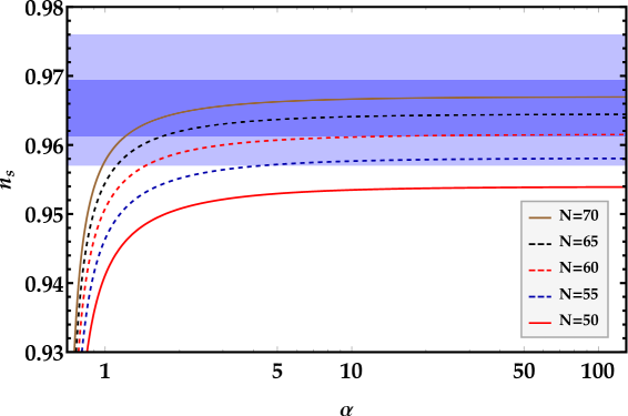
Figure 1: The scalar spectral index $n_{s}$ versus non-canonical parameter $\alpha$ for different $e$-folds number $N=50$ (solid red curve), $N=55$ (dashed blue curve), $N=60$ (dashed red curve), $N=65$ (dashed black curve), and $N=70$ (solid brown curve). The dark and light blue regions show, respectively, the 68% and 95% CL of Planck 2018 TT, TE, EE + LowE + Lensing + BK18 + BAO data.

In Fig. 2, using Eq. (37) the tensor-to-scalar ratio $r$ is depicted in terms of $\alpha$ parameter for various duration of inflationary era. Furthermore, the allowed area for $r$ at 95% CL according to the recent data of Planck’s measurements (22) is marked in light blue in this figure. As depicted in Fig. 2, for $N=70$, the prediction of the model falls within the allowed region for $\alpha\geq 10$. Additionally, the cases associated with smaller $N$ can satisfy observational constraints at higher values of $\alpha$, as it can be seen from Fig. 2.

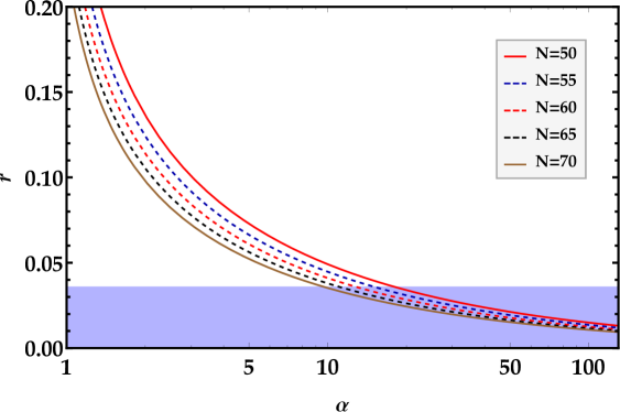
Figure 2: The tensor-to-scalar ratio $r$ versus the non-canonical parameter $\alpha$ for different $e$-folds number $N$. The light blue region shows $r\leq 0.036$ according to Planck 2018 TT, TE, EE + LowE + Lensing + BK18 + BAO at 95% CL.

The allowed ranges for $\alpha$ parameter in $r-n_{s}$ diagram in light of Planck 2018 data for different values of $N$ are shown in Fig. 3 and Table 1. According to these results, for $N=60$, the $\alpha$ parameter must be greater than 18.8 to be in the allowed area. The $f_{\rm NL}^{\rm equil}$ parameter also limits the maximum value of $\alpha$ to 130 in this model (see Table 1).

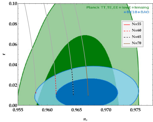
Figure 3: The tensor-to-scalar ratio $r$ versus the scalar spectral index $n_{s}$ with varying $\alpha$ parameter and for different $e$-folds number $N=$ 55 (solid red curve), 60 (dashed red curve), 65 (dashed black curve), and 70 (brown curve). Dark (light) green area represents the 68% (95%) CL of Planck 2018 TT, TE, EE+low E+lensing and dark (light) blue one shows the 68% (95%) CL of Planck 2018 TT, TE, EE+low E+lensing+BK18+BAO in the background.

In Table 1, the computed allowed ranges for the non-canonical parameters $\alpha$ and $\mu$, using the constraints of $c_{s}^{2}+r+n_{s}+f_{\rm NL}^{\rm equil}$ for different $e$-folds number $N$ are expressed. For instance, if the duration of the inflationary era is assumed to be 55 $e$-folds, the $r-n_{s}$ curve is placed within the allowed range of Planck 2018 data for $\alpha\geq 110$. In this calculation, the dimensionless coefficient of self-interaction $\lambda=0.1$ is considered.

Table 1: The allowed ranges for the non-canonical parameters of the model ($\alpha$, $\mu$) according to the constraints of $c_{s}^{2}+r+n_{s}+f_{\rm NL}^{\rm equil}$ for different $e$-folds number $N$.

$N$	$\alpha$	$\mu~{}(\times 10^{-5})$
$55$	$110\leq\alpha\leq 130$	$2.234\leq\mu\leq 2.296$
$60$	$18.8\leq\alpha\leq 130$	$2.071\leq\mu\leq 2.589$
$65$	$11.3\leq\alpha\leq 130$	$1.932\leq\mu\leq 2.339$
$70$	$8.6\leq\alpha\leq 130$	$1.812\leq\mu\leq 2.064$

III Reheating epoch

As mentioned before, at the end of inflation, the kinetic energy of the inflaton overcomes its potential energy. Thence the inflaton oscillates around the minimum of the potential and gradually releases its energy. This epoch is called reheating and its nature is still not fully understood Baumann:2009 . Considering the reheating epoch can also be useful for verifying inflationary models. In this epoch, the equation of state parameter ($\omega_{re}$), the duration of the reheating epoch ($N_{re}$), and the reheating temperature ($T_{re}$) are usually investigated. The duration of reheating epoch and reheating temperature both depend on the equation of state parameter. The most important constraint that the duration of the reheating epoch imposes on the model is that its value must be positive, i.e., $N_{re}>0$. Additionally, the duration of the reheating epoch should be significantly shorter than the duration of the inflation epoch and it can be obtained as follows Mishra:2021 ; Odintsov:2023

$$N_{re}=\left(\frac{4}{1-3\omega_{re}}\right)\left[-\frac{1}{4}\ln\left(\frac{30}{\pi^{2}g_{re}}\right)-\frac{1}{3}\ln\left(\frac{11g_{re}}{43}\right)-\ln\left(\frac{k_{\ast}}{a_{0}T_{0}}\right)-\ln\left(\frac{\rho_{e}^{1/4}}{H_{\ast}}\right)-N\right],$$ (41)

where $g_{re}=106.75$ is the effective number of relativistic degrees of freedom for energy during the reheating epoch, $k_{\ast}=0.05~{}{\rm Mpc^{-1}}$ is the pivot scale, $a_{0}=1$ is the scale factor at the present time, $T_{0}=2.725~{}{\rm K}$ is the current temperature of CMB radiation, $\rho_{e}$ is the energy density of the inflaton field at the end of inflation, $H_{\ast}$ is the Hubble parameter at the horizon crossing time and $N$ defines the duration of inflation from the end of inflation until the horizon passing moment . Using the conversion factor $1~{}{\rm Mpc^{-1}}=6.39\times 10^{-39}{\rm GeV}$, Eq. (41) can be simplified as follows

$$N_{re}=\frac{4}{1-3\omega_{re}}\left[61.6-\ln\left(\frac{\rho_{e}^{1/4}}{H_{\ast}}\right)-N\right],$$ (42)

where the value of $H_{\ast}$ can be estimated from Eq. (14) as follows

$$H_{\ast}=\sqrt{8\pi^{2}M_{p}^{2}c_{s}{\cal P}_{s}(k_{\ast})\epsilon}.$$ (43)

It is known that, the equation of state parameter is defined as

$$\omega_{\phi}\equiv\frac{P_{\phi}}{\rho_{\phi}}=-1-\frac{2}{3}\frac{\dot{H}}{H^{2}}=-1+\frac{2}{3}\epsilon,$$ (44)

where $\epsilon=1$ at the end of inflation. Therefore, the value of the equation of state parameter at the end of inflation is $\omega_{\phi_{e}}=-\frac{1}{3}$, and consequently

$$P_{e}=-\frac{1}{3}\rho_{e}.$$ (45)

By substituting Eqs. (3) and (4) into Eq. (45), the energy density at the end of inflation $\rho_{e}$ in the non-canonical framework with power-law Lagrangian (2) can be obtained by

$$\rho_{e}=\left(\frac{3\alpha}{\alpha-1}\right)V_{e},$$ (46)

where $V_{e}$ is the inflationary potential value at the end of inflation.

According to the calculations of Ref. Unnikrishnan:2012 , for non-canonical action with power-law Lagrangian (2), the equation of state parameter in the reheating epoch can be calculated as follows

$$1+\left\langle\omega_{\phi}\right\rangle=\left(\frac{2\alpha}{2\alpha-1}\right)\left[\int_{0}^{\phi_{m}}{\mathrm{d}\phi\left(1-\frac{V\left(\phi\right)}{V\left(\phi_{m}\right)}\right)}^{\frac{2\alpha-1}{2\alpha}}\right]\left[\int_{0}^{\phi_{m}}{\mathrm{d}\phi\left(1-\frac{V\left(\phi\right)}{V\left(\phi_{m}\right)}\right)}^{\frac{-1}{2\alpha}}\right]^{-1},$$ (47)

where $\langle~{}\rangle$ represents the average value over one oscillation cycle of the inflaton. Similar to the standard inflation in the canonical framework, we assume that the timescale of the scalar field oscillation is much smaller than that of the expansion of the universe. In this limit, the time variations of $\rho_{\phi}$ during each cycle is small enough to approximate $\rho_{\phi}\simeq V(\phi_{m})$, where $\phi_{m}$ is the maximum value of the field during a given cycle. According to Eq. (47), in the framework of non-canonical inflation with a power-law Lagrangian for the potential $V\left(\phi\right)=V_{0}\phi^{n}$, the equation of state parameter can be calculated as follows

$$\omega_{re}=\left\langle\omega_{\phi}\right\rangle=\frac{n-2\alpha}{n\left(2\alpha-1\right)+2\alpha},$$ (48)

which for $n=4$, it can be written as

$$\omega_{re}=\frac{2-\alpha}{5\alpha-2}.$$ (49)

In the following, we calculate the duration of the reheating epoch $N_{re}$ for non-canonical action with power-law Lagrangian (2) and quartic potential (35) by inserting Eqs. (43), (46) and (49) in (42). Then, considering the relation between $n_{s}$ and $N$ from Eq. (36), we plot the values of $N_{re}$ in terms of the scalar spectral index $n_{s}$ in Fig. 4 for different values of $\alpha$ parameter according to Table 1. The red curve in this graph, corresponds to $\alpha=130$ which is obtained from the non-Gaussianity constraint. In this figure, the dark blue, yellow, dashed blue and dashed black curves represent $\alpha=8.6$, $\alpha=11.3$, $\alpha=18.8$, and $\alpha=110$, respectively. The dark (light) blue area indicates the 68% (95%) CL for the scalar spectral index, according to recent data of Planck 2018. It can be observed that despite variations in $\alpha$, there is little difference in the values obtained for the duration of reheating $N_{re}$. In other words, $N_{re}$ is not proportional to changes in $\alpha$. Therefore, in non-canonical framework with quartic potential, $N_{re}$ cannot be a suitable tool to break the degeneracy of the model with respect to $\alpha$ parameter.

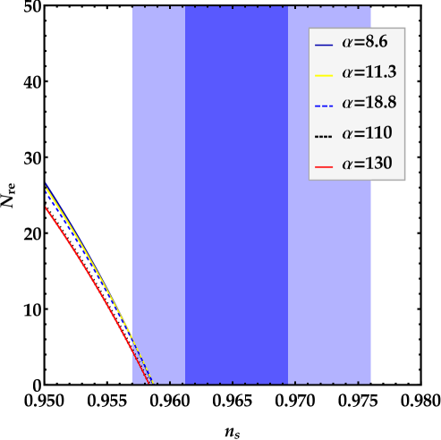
Figure 4: Duration of the reheating stage $N_{re}$ versus the scalar spectral index $n_{s}$ for different values of $\alpha=$ 8.6 (dark blue curve), 11.3 (yellow curve), 18.8 (dashed blue curve), 110 (dashed black curve), and 130 (red curve) according to Table 1. The dark and light blue regions show, respectively, the 68% and 95% CL of Planck 2018 TT, TE, EE + LowE + Lensing + BK18 + BAO data.

In addition to $N_{re}$, the reheating temperature $T_{re}$ can also be used to survey inflationary models and it can be calculated as follows Mishra:2021

$$T_{re}=\left(\frac{45}{\pi^{2}g_{re}}\right)^{1/4}V_{e}^{1/4}\exp\left[-\frac{3}{4}(1+\omega_{re})N_{re}\right].$$ (50)

This parameter depends on $\omega_{re}$, $N_{re}$, and the potential at the end of inflation $V_{e}$. Since the reheating stage occurs after the end of inflation and before the beginning of the Big Bang Nucleosynthesis (BBN) stage, the upper and lower limits on the reheating temperature are defined as follows Mishra:2021 ; Eshaghi:2016 ; LiangDai:2014

$$1\,{\rm MeV}\leq T_{re}\leq 1.6\times 10^{16}\,{\rm GeV}.$$ (51)

In Fig. 5, the reheating temperature $T_{re}$, Eq. (50), is plotted as a function of the scalar spectral index $n_{s}$ for different values of $\alpha$ parameter. The dark (light) blue area represents the 68% (95%) CL specified by Eq. (18) for the scalar spectral index according to recent data of Planck 2018. The gray area at the bottom of the diagram represents the constraint from BBN. The horizontal line at the top of the diagram indicates the upper limit of the reheating temperature. It is worth noting that changing in the $\alpha$ parameter does not yield the significant change in the reheating temperature. Therefore, the reheating temperature in this model, is degenerate with respect to changes in $\alpha$ parameter. It can be inferred from Figs. 4 and 5 that, the duration $N_{re}$ and the temperature $T_{re}$ of the reheating stage cannot impose strict constraints on the free parameters of the inflationary model with a quartic potential in the non-canonical framework. In other words, reheating considerations do not further restrict the values in the parameter space.

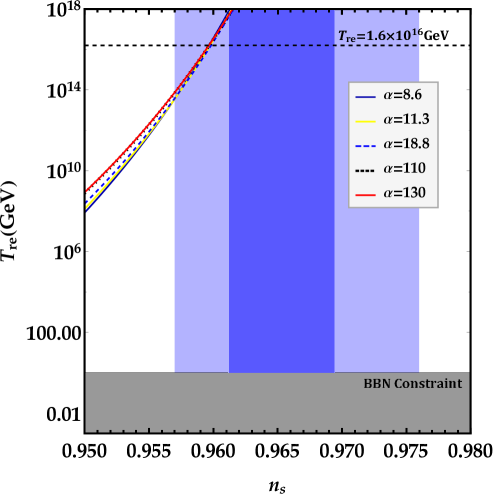
Figure 5: Same as Fig. 4, but for the reheating temperature $T_{re}$. The bottom gray hatched area corresponds to the BBN constraint. The maximum allowable reheating temperature $T_{re}=1.6\times 10^{16}~{}\rm GeV$ is indicated by a horizontal dashed black line at the top of the graph.

IV The relic gravitational waves

Inflation theory predicts that, the primordial tensor fluctuations of the inflaton field can lead to production of gravitational waves (GWs). During inflation, these fluctuations extend beyond the Hubble horizon, and upon reentering, they generate relic GWs Starobinsky:1979 ; allen88 ; sahni:1990 ; sami2002 ; dany_18 ; dany_19 ; Bernal:2019lpc . Due to their weak interaction with matter and radiation, these relic GWs serve as a valuable tool for probing the early universe. The present frequency of the originated relic GWs from the cosmic inflation can be calculated in terms of temperature using the following equation Mishra:2021

$$f=7.36\times 10^{-8}{~{}\rm Hz}\left(\frac{g_{0}^{s}}{g_{T}^{s}}\right)^{\frac{1}{3}}\left(\frac{g_{T}}{90}\right)^{\frac{1}{2}}\left(\frac{T}{\rm GeV}\right),$$ (52)

where $g_{0}^{s}=3.94$ and $g_{T}^{s}=106.75$ are the effective number of relativistic degrees of freedom in entropy at the present time and each epoch with temperature $T$, respectively. Furthermore, $g_{T}=106.75$ is the effective number of relativistic degrees of freedom in energy. The reheating temperature $T_{re}$ and the corresponding frequency of GWs in the reheating epoch $f_{re}$ are listed in Table 2 for several values of $\alpha$ parameter according to Table 1. The present density parameter spectrum of relic GWs in the radiation-dominated and reheating periods are calculated from the following two equations (for more information, see Ref. Mishra:2021 )

$$\mbox{{ Radiation Dominated:}}~{}~{}\Omega_{\rm GW_{0}}^{(\rm RD)}(f)=\left(\frac{1}{24}\right)r~{}{\cal P}_{s}(k_{\ast})\left(\frac{f}{f_{\ast}}\right)^{n_{t}}\Omega_{r_{0}}~{},~{}f_{eq}<f\leq f_{re},\,$$ (53)

$$\mbox{{reheating:}}~{}~{}\Omega_{\rm GW_{0}}^{(\rm re)}(f)=\Omega_{\rm GW_{0}}^{(\rm RD)}(f)\left(\frac{f}{f_{re}}\right)^{2\left(\frac{\omega_{re}-1/3}{\omega_{re}+1/3}\right)},~{}~{}f_{re}<f\leq f_{e}\,,$$ (54)

where $\Omega_{r_{0}}=2.47\times 10^{-5}h^{-2}$ is the radiation density parameter at present time, $f_{*}=2.4\times 10^{-16}~{}({\rm Hz})$ is the frequency of GWs at the CMB pivot scale $k_{\ast}=0.05~{}{\rm Mpc^{-1}}$, $f_{eq}=1.7\times 10^{-17}~{}({\rm Hz})$ represents the frequency of GWs at the matter-radiation equality and $f_{e}=4.3\times 10^{8}~{}({\rm Hz})$ is the frequency of GWs at the end of inflation.

Table 2: The allowed regions of the reheating temperature $T_{re}^{\rm min}\leq T_{re}\leq T^{\rm max}_{re}=1.6\times 10^{16}~{}\rm GeV$ and the corresponding frequency $f_{re}^{\rm min}\leq f_{re}\leq f^{\rm max}_{re}=4.3\times 10^{8}~{}\rm Hz$ of GWs in the reheating epoch computed by Eq. (52) for several values of $\alpha$ parameter according to Fig. 5 (or Table 1).

$\alpha$	$T_{re}^{\rm min}~{}(\times 10^{13}~{}{\rm GeV})$	$f_{re}^{\rm min}~{}(\times 10^{6}~{}{\rm Hz})$
$8.6$	$3.49$	$0.93$
$11.3$	$3.48$	$0.93$
$18.8$	$3.79$	$1.01$
$110$	$6.97$	$1.86$
$130$	$7.46$	$1.99$

In Fig. 6, the present density parameter spectra of GWs are plotted in four graphs, for different durations of inflationary era as 55, 60, 65, and 70 $e$-folds, using Eqs. (52)-(54). The green area represents the sensitivity range of the Big Bang Observer (BBO) gravitational wave detector Yagi:2011 ; BBO:2003 , while the red area represents the sensitivity range of the DECi-hertz Interferometer Gravitational-wave Observatory (DECIGO) detector Yagi:2011 ; Seto:2001 . The black vertical lines in all graphs indicate the frequencies of GWs calculated for specific reheating temperatures according to Table 2. The solid red lines in all graphs represent the present energy density of GWs computed for the quartic potential in the non-canonical framework for $\alpha=130$. The blue line in each graph represents the present energy density of GWs for the lowest limit of $\alpha$ parameter according to Table 1. Each graph corresponds to a specific duration of the inflation epoch. It can be observed that all plots fall within the sensitivity range of GWs detectors. Hence, with the advancement of these detectors, there is a possibility of detecting the predicted relic GWs by this model. Moreover, varying in $\alpha$ parameter leads to distinct values of relic GWs density. Therefore, the analysis of the relic GWs can break the degeneracies of the predictions of the non-canonical inflationary model, containing the quartic potential (35) and power-law Lagrangian (2), with respect to the $\alpha$ parameter.

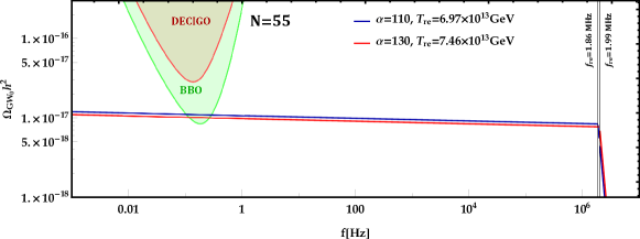
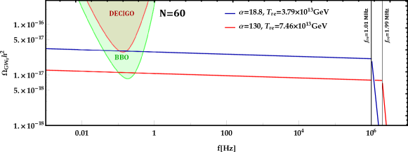
Figure 6: Present density parameter spectra of GWs versus frequency for different values of $\alpha$ parameter, considering different duration for inflationary era as 55, 60, 65 and 70 $e$-folds. The hatched regions represent the sensitivity ranges of BBO and DECIGO GWs detectors. The red line in each graph denotes the present density parameter spectrum of GWs for $\alpha=130$, while the blue line corresponds to the lowest limit of $\alpha$ parameter according to Table 1. The vertical black lines indicate the frequencies of GWs calculated for a specific reheating temperature according to Table 2.

V Conclusion

In this work, we investigated the quartic potential in non-canonical inflationary model with power-law Lagrangian (2). We showed that, in contrary to the standard inflation, the predictions of this potential in non-canonical framework are consistent with the observational data of Planck 2018. Among the free parameters of the model, only the changes of $\alpha$ parameter have a significant effect on the predictions of the model.

We checked the model based on the changes of $\alpha$ considering different values for the duration of the inflation epoch $N$. To determine the allowed range of $\alpha$ parameter, we used theoretical considerations as well as observational constraints. We showed that the sound speed parameter $c_{s}$, equilateral non-Gaussianity $f_{\rm NL}^{\rm equil}$, scalar spectral index $n_{s}$, and tensor-to-scalar ratio $r$ bound the parameter $\alpha$ (see Table 1). The minimum value of $\alpha$ was determined to be larger than $1/2$ based on the constraint on $c_{s}$. The equilateral non-Gaussianity constraint also limits the maximum value of $\alpha$ to be $\alpha\leq 130$. The $r-n_{s}$ curve sets the lower bound on $\alpha$ considering specific duration for inflation. For example, for $N=60$ we obtain $\alpha\geq 18.8$.

Then, we examined the observational predictions of the model for $n_{s}$ and $r$ with respect to $\alpha$ parameter. It was found that, the scalar spectral index of this model shows degeneracy at large values of $\alpha$ parameter (see Fig. 1). In the following, we examined three parameters of the reheating epoch, including the equation of state parameter $\omega_{re}$, the duration of the reheating epoch $N_{re}$, and the temperature of the reheating epoch $T_{re}$. We examined $N_{re}$ and $T_{re}$ in terms of $n_{s}$ for several values of $\alpha$. We showed that by varying $\alpha$, the obtained values for both $N_{re}$ and $T_{re}$ in terms of $n_{s}$ do not exhibit much differentiation and are somewhat degenerate. Therefore, the parameters of the reheating epoch are not sensitive to the changes of $\alpha$ (see Figs. 4 and 5). For this reason, we examined the relic GWs for this model. We checked the present density of the relic GWs for different values of $\alpha$ parameter and durations of inflation between 55 to 70 $e$-folds. We found that, the present density parameter of the relic GWs is sensitive to changes in $\alpha$ parameter. So using the relic GWs considerations, the degeneracy of the model with respect to $\alpha$ parameter can be broken. Moreover, we showed that the present density of relic GWs for this model, falls within the sensitivity ranges of developing GWs detectors.

Acknowledgements

The authors thank Soma Heydari and Milad Solbi for valuable discussions.

References

- (1) A. A. Starobinsky, A New Type of Isotropic Cosmological Models Without Singularity, Phys. Lett. B 91, 99 (1980).
- (2) A. H. Guth, The Inflationary Universe: A Possible Solution to the Horizon and Flatness Problems, Phys. Rev. D 23, 347 (1981).
- (3) A. D. Linde, A New Inflationary Universe Scenario: A Possible Solution of the Horizon, Flatness, Homogeneity, Isotropy and Primordial Monopole Problems, Phys. Lett. B 108, 389 (1982).
- (4) A. Albrecht and P. J. Steinhardt, Cosmology for Grand Unified Theories with Radiatively Induced Symmetry Breaking, Phys. Rev. Lett. 48, 1220 (1982).
- (5) A. D. Linde, Particle Physics and Inflationary Cosmology, Harwood, Chur, Switzerland (1990).
- (6) D. Baumann, Inflation, in Theoretical Advanced Study Institute in Elementary Particle Physics: Physics of the Large and the Small, 7, 2009, DOI [arXiv:0907.5424].
- (7) A. R. Liddle and D. H. Lyth, Cosmological inflation and large scale structure, Cambridge University Press, Cambridge U.K. (2000).
- (8) P. A. R. Ade et al. (Keck Array and bicep Collaborations), Constraints on Primordial Gravitational Waves Using Planck, WMAP, and New BICEP2/Keck Observations through the 2015 Season, Phys. Rev. Lett. 121, 221301 (2018).
- (9) R. Kallosh and A. Linde, Universality Class in Conformal Inflation, J. Cosmol. Astropart. Phys. 07, 002 (2013).
- (10) R. Kallosh, A. Linde, and D. Roest, Superconformal Inflationary -Attractors, J. High. Energy. Phys. 11 , 198 (2013).
- (11) Y. Akrami et al. (Planck Collaboration), Planck 2018 results, IX. Constraints on primordial non-Gaussianity, Astron. Astrophys. 641, A9 (2020).
- (12) L. P. Grishchuk, Amplification of gravitational waves in an istropic universe, Zh. Eksp. Teor. Fiz. 67, 825 (1974).
- (13) A. A. Starobinsky, Spectrum of relict gravitational radiation and the early state of the universe, JETP Lett. 30 682 (1979).
- (14) A. A. Starobinsky, Evolution of small perturbations of isotropic cosmological models with one-loop quantum gravitational corrections, J. Exp. Theor. Phys. 34, 438 (1981).
- (15) L. Kofman, A. D. Linde, and A. A. Starobinsky, Reheating after inflation, Phys. Rev. Lett. 73, 3195 (1994).
- (16) L. A. Kofman, The Origin of matter in the universe: Reheating after inflation, 5, 1996, arXiv:astro-ph/9605155.
- (17) J. Martin and C. Ringeval, First CMB Constraints on the Inflationary Reheating Temperature, Phys. Rev. D 82, 023511 (2010).
- (18) L. Dai, M. Kamionkowski, and J. Wang, Reheating constraints to inflationary models, Phys. Rev. Lett. 113, 041302 (2014).
- (19) M. Eshaghi, M. Zarei, N. Riazi, and A. Kiasatpour, CMB and reheating constraints to -attractor inflationary models, Phys. Rev. D 93, 123517 (2016).
- (20) S. S. Mishra, V. Sahnia, and A. A. Starobinsky, Curing inflationary degeneracies using reheating predictions and relic gravitational waves, J. Cosmol. Astropart. Phys. 05, 075 (2021).
- (21) S. Unnikrishnan, V. Sahni, and A. Toporensky, Refining inflation using non-canonical scalars, J. Cosmol. Astropart. Phys. 08, 018 (2012).
- (22) K. Rezazadeh, K. Karami, and P. Karimi, Intermediate in ation from a non-canonical scalar field, J. Cosmol. Astropart. Phys. 09, 053 (2015).
- (23) S. Heydari and K. Karami, Primordial black holes in non-canonical scalar field inflation driven by quartic potential in the presence of bump, J. Cosmol. Astropart. Phys. 02, 047 (2024).
- (24) S. Heydari and K. Karami, Primordial black holes and secondary gravitational waves from generalized power-law non-canonical inflation with quartic potential Eur. Phys. J. C 84, 127 (2024).
- (25) S. S. Mishra and V. Sahni, Canonical and Non-canonical Inflation in the light of the recent BICEP/Keck results, arXiv:2202.03467.
- (26) G. Panotopoulos, Detectable primordial non-Gaussianities and gravitational waves in k-inflation, Phys. Rev. D 76, 127302 (2007).
- (27) J. Garriga and V. F. Mukhanov, Perturbations in k-inflation, Phys. Lett. B 458, 219 (1999).
- (28) P. A. R. Ade et al. (BICEP/Keck Collaboration), Improved Constraints on Primordial Gravitational Waves using Planck, WMAP, and BICEP/Keck Observations through the 2018 Observing Season, Phys. Rev. Lett. 127, 151301 (2021).
- (29) D. Paoletti, F. Finell, J. Valiviita, and M. Hazumi, Planck and BICEP/Keck Array 2018 constraints on primordial gravitational waves and perspectives for future B-mode polarization measurements Phys. Rev. D 106, 083528 (2022).
- (30) Y. Akrami et al. (Planck Collaboration), Planck 2018 results, VI. Cosmological parameters, Astron. Astrophys. 641, A10 (2020).
- (31) M. Tanabashi et al., Review of Particle Physics, Phys. Rev. D 98, 030001 (2018).
- (32) R. L. Workman et al. (Particle Data Group), Review of Particle Physics, Prog. Theor. Exp. Phys. 2022, 083C01 (2022).
- (33) X. Chen, M. X. Huang, S. Kachru, and G. Shiu, Observational signatures and non-Gaussianities of general single-field inflation, J. Cosmol. Astropart. Phys. 01, 002 (2007).
- (34) S. D. Odintsov and T. Paul, From inflation to reheating and their dynamical stability analysis in Gauss–Bonnet gravity, Phys. of the Dark Universe 42, 101263 (2023).
- (35) V. Sahni, Energy density of relic gravity waves from inflation, Phys. Rev. D 42, 453 (1990).
- (36) B. Allen, Stochastic gravity-wave background in inflationary-universe models, Phys. Rev. D 37, 2078 (1988).
- (37) C. Caprini and D. G. Figueroa, Cosmological backgrounds of gravitational waves, Class. Quant. Grav. 35, 163001 (2018).
- (38) D. G. Figueroa and E. H. Tanin, Ability of LIGO and LISA to probe the equation of state of the early Universe, J. Cosmol. Astropart. Phys. 08, 011 (2019).
- (39) N. Bernal and F. Hajkarim, Primordial gravitational waves in nonstandard cosmologies, Phys. Rev. D 100, 063502 (2019).
- (40) V. Sahni, M. Sami, and T. Souradeep, Relic gravity waves from braneworld inflation, Phys. Rev. D 65, 023518 (2001).
- (41) K. Yagi and N. Seto, Detector configuration of DECIGO/BBO and identification of cosmological neutron-star binaries, Phys. Rev. D 83, 044011 (2011).
- (42) S. Phinney et al., The Big Bang Observer: Direct detection of gravitational waves from the birth of the Universe to the Present, NASA mission concept study (2004).
- (43) N. Seto, S. Kawamura, and T. Nakamura, Possibility of Direct Measurement of the Acceleration of the Universe Using 0.1 Hz Band Laser Interferometer Gravitational Wave Antenna in Space, Phys. Rev. Lett. 87, 221103 (2001).