Towards Atomic MIMO Receivers

Abstract

The advancement of Rydberg atoms in quantum information technology is driving a paradigm shift from classical radio-frequency (RF) receivers to atomic receivers. Capitalizing on the extreme sensitivity of Rydberg atoms to external electromagnetic fields, atomic receivers are capable of realizing more precise radio-wave measurements than RF receivers to support high-performance wireless communication and sensing. Although the atomic receiver is developing rapidly in quantum-physics domain, its integration with wireless communications is at a nascent stage. In particular, systematic methods to enhance communication performance through this integration are yet to be discovered. Motivated by this observation, we propose in this paper to incorporate atomic receivers into multiple-input-multiple-output (MIMO) communication, a prominent 5G technology, as the first attempt on implementing atomic MIMO receivers. To begin with, we provide a comprehensive introduction on the principles of atomic receivers and build on them to design the atomic MIMO receivers. Our findings reveal that signal detection of atomic MIMO receivers corresponds to a non-linear biased phase retrieval (PR) problem, as opposed to the linear Gaussian model adopted in classical MIMO systems. Then, to recover signals from this non-linear model, we modify and integrate the Gerchberg-Saxton (GS) algorithm, a typical PR solver, with a biased GS algorithm to solve the biased PR problem. Moreover, we propose a novel Expectation-Maximization GS (EM-GS) algorithm to cope with the unique Rician distribution of the biased PR model. Our EM-GS algorithm introduces a high-pass filter constructed by the ratio of Bessel functions into the iteration procedure of GS, thereby improving the detection accuracy without sacrificing the computational efficiency. Finally, the effectiveness of the devised algorithms and the feasibility of atomic MIMO receivers are demonstrated by theoretical analysis and numerical simulation.

I Introduction

With the global deployment of commercial 5G services, cutting-edge research on 6G has been launched worldwide [1]. Meanwhile, the revolutionary quantum information technologies are evolving rapidly and deemed as a key enabler of the next-generation computing, communication, and sensing [2, 3, 4]. For example, ever since the invention of Schor’s algorithm, quantum computing has exhibited unparalleled abilities in quadratically or even exponentially accelerating the computing speed in solving classically intractable problems, ranging from factorization to optimization to artificial intelligence [2]. On the other hand, leveraging quantum mechanisms such as superposition and entanglement, quantum communication is capable of establishing unconditionally secure links to protect data privacy [3]. In parallel with communication and computing, quantum sensing is another promising branch of quantum information technologies [4]. It employs microscopic particles as “sensors” and capitalizes on their strong sensitivity to external disturbance, especially electromagnetic fields, to precisely measure some physical quantities. Notable examples of quantum sensors include atomic clocks and superconducting interferometers. As an exciting trend, quantum sensors are being applied to an increasingly broad range of practical use cases [4, 5, 6]. Relevant techniques promise to reshape the information society and our perception of the environment. Aligned with this end, our work advocates the use of quantum sensors to revolutionize next-generation wireless receivers.

I-A Concept and Properties of Atomic Receiver

Recently, at the intersection of quantum sensing and wireless communications, an emerging concept known as atomic receiver has attracted extensive attentions, for their capabilities of high-precision measurement of electromagnetic fields [5]. An atomic receiver leverages Rydberg atoms as “antennas” to detect the amplitude, phase, frequency, and polarization of incident electromagnetic waves [7]. To elaborate, Rydberg atoms refer to highly excited atoms, whose outermost electrons are excited to high energy levels far from their nuclei [8]. Attributed to their large electric dipole moments and high polarizability, such atoms are extremely sensitive to external electromagnetic fields, rendering them excellent “atomic antennas”. To implement wireless receivers, a modulated electromagnetic wave first interacts with Rydberg atoms to trigger their electronic transitions between certain energy levels. The resultant intensity of electron transition can be monitored using an all-optical readout mechanism, termed the electromagnetically induced transparency (EIT), to facilitate the ensuing information demodulation [5]. In contrast with the macroscopic measurement of electromagnetic fields by conventional radio-frequency (RF) receivers, the atomic counterparts operate at the atom-scale microcosm. This fundamentally different principle enables the latter to achieve accuracies at the quantum limit and have the potential of working in tandem with or even replacing conventional RF receivers[9].

Benefiting from the advancements in quantum sensing, atomic receivers offer several advantages over conventional receivers for wireless communication and sensing. First, atomic receivers can achieve much higher detection-and-sensing accuracies as mentioned earlier [4]. For example, as demonstrated in [6], atomic receivers can achieve the sub-millimeter (sub-mmWave) level granularity in detecting object vibrations using WiFi sources as opposed to the mmWave level granularity attained by traditional receivers. The second advantage lies in low thermal noise. Conventional receivers require RF circuits to intercept radio waves and downconvert RF signals to the baseband, which comprise components such as RF antennas, analog filters, and mixers that generate significant thermal noise. In contrast, atomic receivers employ all-optical components for sensing and downconversion, and thus are immune to thermal noise [7]. The above two advantages make atomic receivers a promising technology for long-range communications [5]. Last but not the least, the flexible tunability of Rydberg atoms across an ultra-wide spectrum is a significant advantage [9]. Traditional antennas, with a fixed size typically half the wavelength of the carrier, are limited in the spectrum bandwidth they can listen to. Detecting multi-band signals requires an array of costly RF receivers, each of which is matched to a specific band [10]. In contrast, the numerous energy levels in Rydberg atoms allow an atomic receiver to respond to a broad range of frequencies from 100 Megahertz (MHz) to 1 Terahertz (THz) by exciting electrons to different energy levels [11]. This capability enables the simultaneous measurement of multi-band signals over an extremely wide spectrum using a single atomic receiver, laying the foundation for constructing an extraordinarily cost-effective full-frequency communication platform. To materialize the above visions, this work incorporates atomic receivers into modern wireless communication systems.

I-B State-of-the-art Atomic Receivers

Existing research on atomic receivers primarily focuses on the lab demonstrations of different signal modulation schemes. It is well-known that via the interaction between electromagnetic fields and Rydberg atoms, the strength and frequency of modulated radio waves can be transduced into the intensity of electron transition, called the Rabi frequency. Hence, by inferring symbols from the Rabi frequencies, both the amplitude demodulation and frequency demodulation at $37.4$ GHz and $29.5$ GHz have been realized, respectively [12]. For phase demodulation, researchers employed the holographic phase-sensing methodology, involving the use of a local oscillator (LO) to generate a reference electromagnetic field with a known phase that interferes with the incident modulated electromagnetic field [13, 14, 15]. Then, the phase-modulated symbols can be extracted from the phase differences between the aforementioned fields. In [16], a channel capacity of up to 8.2 Mbps was measured using the 8-state phase-shift-keying modulation. This holographic principle was then extended to support angle-of-arrival estimation [17] and micro-vibration monitoring [6]. Another vein of research exploits the capability of atomic receivers for multi-band communications [11, 18]. For example, it was proposed in [18] to excite electrons to the same initial Rydberg energy level but transfer them to different final Rydberg energy levels via the interaction with separate frequency bands. This approach enables the co-detection of 5 frequency bands at 1.72, 12.11, 27.42, 65.11, and 115.75 GHz.

Despite the rapid development of atomic receivers in the quantum-sensing domain, their application in wireless communication is still at a nascent stage. The state-of-the-art designs are suitable only for primitive communication scenarios and schemes, such as a point-to-point system or a single-input-single-output (SISO) air interface. Without advanced designs and advices, the full potential of atomic receivers cannot be unleashed, with the state-of-the-art achieving only a Mbps-scale channel capacity [16, 11, 18]. Communication techniques that are customized for atomic receivers are largely uncharted. This calls for research on atomic-level channel coding, massive multiple-input-multiple-output (MIMO), multi-user communications, integrated sensing and communication (ISAC), reconfigurable intelligent surface (RIS), and edge learning [19, 20, 21]. To contribute to this emerging field, this paper seeks the feasibility of integrating MIMO communications and atomic receivers. MIMO, a key 5G technology, features spatial multiplexing of parallel data links and enhancement of link reliability via diversity gain [19]. It is believed that the consideration of MIMO has the potential to overcome the capacity bottleneck of current atomic SISO receivers.

I-C Contributions and Organization

To the best of our knowledge, this work represents the first attempt on designing and analyzing atomic MIMO receivers. We propose a novel framework for atomic MIMO receiver by building on the basic mechanisms of quantum sensing. In this framework, phase-modulated symbols simultaneously transmitted by multiple users are detected by multiple atomic antennas using the mentioned scheme of holographic phase-sensing. The key contributions and findings are summarized as follows.

• Modeling of atomic MIMO receiver: Our model of atomic MIMO receiver reveals that its signal detection is essentially a biased phase retrieval (PR) problem. In particular, the transmitted symbols are modulated in the coupling strength between the electric dipole moment of Rydberg atoms and the incident radio waves from the users and the reference source. The atomic MIMO receiver capitalizes on this strength to infer multi-user symbols without the help of phase information. This finding highlights one crucial departure of atomic MIMO system from its traditional counterpart: as opposed to the linear transmission model fitting the latter, the former operates in a non-linear transmission model.

• Signal detection for atomic MIMO receiver: To solve the discovered biased PR problem, we propose two signal detection algorithms: the biased Gerchberg-Saxton (GS) and the Expectation-Maximization GS (EM-GS) algorithms, which are based on the least square (LS) and maximum likelihood (ML) criteria, respectively. First, the biased GS algorithm extends the classic GS algorithm [22], a popular PR solver, by eliminating the bias caused by the reference source in the initialization and iteration steps of the classic algorithm. Next, the proposed EM-GS algorithm employs the Bayesian regression to perform ML detection. Its novelty lies in treating the unobserved phase information as a latent variable and thereby decoupling the intricate ML problem into a sequence of tractable linear regression problems with analytical solutions. A comparison of the proposed EM-GS algorithm to the biased GS algorithm reveals that the former features an additional high-pass filter as constructed by the ratio of Bessel functions. This entails the improvement of detection accuracy without increasing computational complexity.

• Performance study: We employ two metrics, namely the normalized mean square error (NMSE) and the bit error ratio (BER), to validate the feasibility of atomic MIMO receivers as well as the effectiveness of the proposed algorithms. Targeting the NMSE metric, the Cramér-Rao lower bound (CRLB) is derived. Numerical results demonstrate that the proposed EM-GS algorithm consistently approaches the CRLB and outperforms the biased GS algorithm, especially in the low signal-to-noise ratio (SNR) regime. Regarding the BER performance, simulation results confirm that the biased GS and EM-GS algorithms achieve BERs close to those from an exhaustive search, while being much more computational efficient.

The remainder of this paper is organized as follows. The preliminaries of atomic SISO receivers are provided in Section II. The framework of atomic MIMO receiver and the corresponding detection algorithms are presented in Section III and Section IV, respectively. In Section V, we validate the proposed design by numerical results. Finally, conclusions are drawn in Section VI.

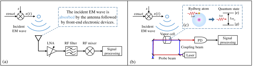
Figure 1: Wireless communication systems based on (a) classical receiver and (b) atomic receiver. (c) Rydberg atoms and energy level diagram.

II Preliminaries of Atomic Wireless Receiver

To help understanding of the proposed framework, preliminaries of atomic receiver for a SISO air interface is provided in this section. We first present the architecture of an atomic receiver and explain the underlying physical laws of Rydberg atoms as antennas, followed by an introduction to quantum jump enabling wireless signal detection. Last, we end this section with the implementation of atomic receivers.

II-A Atomic Receiver Architecture

To begin with, the wireless communication systems employing classical and atomic receivers are differentiated in Fig. 1. The two systems are identical in terms of transmitter architecture and channel. Specifically, data symbols are pre-processed using electronic circuits and modulated onto electromagnetic waves. Their distinction lies in the receiver architecture as elaborated in the sequel. A classical receiver utilizes a dipole antenna to transduce incident waves into signals and decodes from them transmitted bits using a series of electronic components, such as mixers, amplifiers, filters, and baseband professors. In contrast, an atomic receiver employs a different signal-detection paradigm. Such a receiver deploys Rydberg atoms as its “antennas” to measure the amplitude, phase, frequency, and polarization of an electromagnetic field, leveraging their exceptional sensitivity to electromagnetic waves ranging from MHz to THz. Free from energy-consuming and bulky electronic components, a vapor cell filled with Rydberg atoms suffices for sensing the wireless environment. The underpinning mechanism involves the incident electromagnetic wave interacting with Rydberg atoms to change their quantum states, which are monitored using an all-optical readout device, such as a photodetector (PD). The output is processed by a signal-detection algorithm to decipher the transmitted bits. In summary, the architecture of an atomic-receiver based communication system comprises a classic transmitter, a classic channel, and a quantum receiver.

II-B Rydberg Atoms as Antennas

II-B1 Atomic Energy Levels

To grasp the concept of atomic receiver, it is essential to first understand the principle of Rydberg atoms. Each atom consists of a positively charged nucleus surrounded by multiple negatively charged electrons. According to the Rutherford–Bohr model, the Coulomb potential from the nucleus confines the electrons to discrete orbits with distinct energy levels [23]. An energy level can be denoted as $n\ell_{j}$, where $n$, $\ell$, and $j$ represent the principal quantum number, the orbit angular momentum quantum number, and the total angular momentum quantum number, respectively [24]. While $n$ and $j$ are numerical, $\ell$ is assigned a letter from $S,P,D,F,\cdots,$ in an ascending order according to the spectroscopic notation. For instance, $n\ell_{j}=50P_{1/2}$. Let $E_{n\ell j}$ denote the energy corresponding to the energy level $n\ell_{j}$. In particular, for a hydrogen-like atom,

$$E_{n\ell j}=-\frac{hc{\rm Ry}}{(n-\delta_{nlj})^{2}},$$ (1)

where $h=6.626\times 10^{-34}$ J$\cdot$s is the Planck constant, $c=2.998\times 10^{8}$ m$\cdot$s^-1 the speed of light, ${\rm Ry}=1.079\times 10^{7}$ m^-1 the Rydberg constant, and $\delta_{nlj}$ the quantum defect constant specific for each energy level [5]. For ease of notation, we omit the subscript $\ell j$ of $E_{n\ell j}$ in the sequel. Besides, it is useful to define the intrinsic frequency of each energy level as $\omega_{n}\overset{\Delta}{=}\frac{E_{n}}{\hbar}$, and the transition frequency between two energy levels as $\omega_{nm}\overset{\Delta}{=}\omega_{n}-\omega_{m}=\frac{E_{n}-E_{m}}{\hbar}$, where $\hbar=\frac{h}{2\pi}$ is the reduced Planck constant.

II-B2 Quantum Jump

Electrons can jump between energy levels by either absorbing or emitting photons [25]. When a photon is absorbed, the electron is excited to a higher energy level, while transitioning to a lower energy level results in photon emission. This peculiar quantum phenomenon is known as quantum jump or electron transition. It is worth mentioning that the electromagnetic radiation/sensing essential for wireless communication is a special form of photon emission/absorption due to the wave–particle duality [24]. The energy conservation law dictates that an electron transition between two energy levels $E_{n}$ and $E_{m}$ ($E_{n}>E_{m}$) can occur only when the angular frequency $\omega$ of electromagnetic wave is close to the transition frequency, $\omega_{nm}$, (i.e., near-resonance or resonance). The quantum jumps in response to carrier frequencies are the fundamental phenomenon enabling atomic receivers.

II-B3 Definition of Rydberg Atom

An atom becomes a Rydberg atom when at least one of its electrons is excited to a high energy level (Rydberg state) with a principal quantum number $n>20$ [8]. As depicted in Fig. 1(b), to prepare Rydberg atoms, two laser beams of different frequencies and intensities (i.e., a weak probe beam and a strong coupling beam) are steered in opposite directions to propagate through a vapor cell filled with alkali-metal atoms [12]. The probe beam excites the outermost electrons from their ground level to a low excited state (e.g., $6S_{1/2}\rightarrow 6P_{1/2}$). The coupling beam then further triggers these electrons to jump from the state to a highly excited Rydberg state (e.g., $6P_{1/2}\rightarrow 47S_{1/2}$), thereby creating Rydberg atoms. Apart from the preparation of Rydberg states, the probe beam also serves the purpose of reading out the quantum state of Rydberg atoms, as elaborated in Section II-E.

II-B4 Properties of Rydberg Atom

Rydberg atoms exhibit several properties useful for wireless communication due to the large electron-nucleus separation distance. First, Bohr’s model indicates that the orbit radius of an electron is proportional to $n^{2}$ [8]. The large principal quantum number in a Rydberg atom results in a large atomic radius and, consequently, makes Rydberg atoms extremely sensitive to incident electromagnetic waves, enabling accurate signal detection. Second, it follows from (1) that the energy spacing between two adjacent energy levels is approximately $\Delta E\propto\frac{1}{n^{3}}$. This scaling reveals that energy levels become denser with increasing $n$. As a result, the set of available transition frequencies $\omega_{nm}$ becomes larger to cover a wide range of spectrum from MHz to THz [6]. For example, the transition between energy levels $52D_{5/2}$ and $53P_{3/2}$ corresponds to a transition frequency $\omega_{nm}=2\pi\times 5$ GHz, which falls within the sub-6G band. On the other hand, mmWave signals at $28$ GHz can trigger the transition between energy levels $61D_{5/2}$ and $63P_{1/2}$. The preceding advantages inspire researchers to develop atomic receivers based on Rydberg atoms to realize wireless detection across a vast range of communication bands [11, 18].

II-C Electromagnetic Wave and Quantum Jump

II-C1 Quantum State of Rydberg Atom

Let $P$ and $s$ denote transmit power and baseband signal in a narrowband system, respectively. Consider the system in Fig. 1(b), the incident electromagnetic wave at the receiver is given as

$${\mathbf{E}}(t)=\bm{\epsilon}\sqrt{P}\rho s\cos(\omega t+\varphi),$$ (2)

where $\rho$ represents the path loss, $\varphi$ the phase shift, and the unit-vector, $\bm{\epsilon}=[\epsilon_{x},\epsilon_{y},\epsilon_{z}]^{T}$ with $\|\bm{\epsilon}\|_{2}=1$, the polarization direction. The receiver relies on a vapor cell filled with Rydberg atoms to detect the wave by observing the atoms’ quantum jumps. Specifically, the energy conservation law states that if we shine an atom with an electromagnetic wave of frequency $\omega$, its quantum jumps are primarily between two energy levels, namely the ground state, $E_{g}=\hbar\omega_{g}$, and the excited state, $E_{e}=\hbar\omega_{e}$, where $\omega_{e}>\omega_{g}$ and $\omega\approx\omega_{eg}=\omega_{e}-\omega_{g}$ [25]. Accordingly, the quantum state of this two-level system is represented by a $2\times 1$ complex vector. To be specific, the ground state and excited state are represented as $\ket{g}=[0,1]^{T}$ and $\ket{e}=[1,0]^{T}$, respectively, which serve as the orthogonal basis of this system. A general quantum state, $\ket{\psi}$, is modeled by the linear combination of $\ket{g}$ and $\ket{e}$:

$$\ket{\psi}=\alpha_{g}\ket{g}+\alpha_{e}\ket{e}=[\alpha_{e},\alpha_{g}]^{T},$$ (3)

where the complex coefficients, $\alpha_{g}$ and $\alpha_{e}$, are called the probability amplitudes of $\ket{\psi}$, satisfying $|\alpha_{g}|^{2}+|\alpha_{e}|^{2}=1$. When $\ket{\psi}$ is measured on the basis $\{\ket{g},\ket{e}\}$, the outcome is $\ket{g}$ with probability $|\alpha_{g}|^{2}$ and $\ket{e}$ with probability $|\alpha_{e}|^{2}$.

II-C2 State Evolution of Rydberg Atom

For a time-varying system we consider, i.e., $\ket{\psi(t)}=\alpha_{g}(t)\ket{g}+\alpha_{e}(t)\ket{e}$, the evolution of quantum state is governed by the Schrödinger equation [24]:

$$i\hbar\frac{\partial\ket{\psi(t)}}{\partial t}=(\hat{H}+\hat{V})\ket{\psi(t)},$$ (4)

where $i=\sqrt{-1}$, and the operators $\hat{H}$ and $\hat{V}$ are known as the free Hamiltonian and interaction Hamiltonian operators, which represent the energy of the isolated atom and interaction between the incidence wave and atom, respectively. The detailed descriptions and mathematical expressions can be found in Appendix A.

Assume the initial state is $\alpha_{g}(0)=1$ and $\alpha_{e}(0)=0$. Given the definitions of $\hat{H}$ and $\hat{V}$ in Appendix A, we can solve the Schrödinger equation in (4) using the method of rotating-wave approximation (see details in [25]). As a result, the probability, $|\alpha_{e}(t)|^{2}$, can be derived as

$$|\alpha_{e}(t)|^{2}=\frac{\Omega_{R}^{2}}{\Omega_{R}^{2}+\delta^{2}}\sin^{2}\left(\frac{\sqrt{\Omega_{R}^{2}+\delta^{2}}}{2}t\right),$$ (5)

where $\delta\overset{\Delta}{=}\omega_{eg}-\omega$ denotes the detuning of the carrier frequency $\omega$ from the transition frequency $\omega_{eg}$. In (5), $\Omega_{R}\overset{\Delta}{=}\frac{|({\mathbf{r}}_{eg}^{T}\bm{\epsilon})q\sqrt{P}\rho s|}{\hbar}$ denotes the Rabi frequency, defined as the frequency at which the probability amplitudes of two atomic energy levels fluctuate in response to an oscillating electromagnetic field [25]. The vector ${\mathbf{r}}_{eg}=\bra{e}\hat{{\mathbf{r}}}\ket{g}$ defined in Appendix A is determined by the energy levels, where $\hat{{\mathbf{r}}}$ denotes the position operator of an atom. Besides, the inner product ${\mathbf{r}}_{eg}^{T}\bm{\epsilon}$ in $\Omega_{R}$ is called the dipole matrix element [23]. For ease of notation, we introduce $\Omega\overset{\Delta}{=}\sqrt{\Omega^{2}_{R}+\delta^{2}}$ to represent the effective Rabi frequency.

The oscillation at the Rabi frequency as depicted in (5), known as Rabi oscillation, results from electrons’ back-and-forth transitions between ground and excited states. This causes time-variation of electron populations over energy levels. When the carrier frequency exactly matches the transition frequency (i.e., $\omega=\omega_{eg}$), the excited-state probability in (5) is simplified as $|\alpha_{e}(t)|^{2}=\sin^{2}\left(\frac{\Omega_{R}}{2}t\right)$ with the oscillation magnitude at its maximum of one. On the other hand, as the carrier frequency $\omega$ deviates from $\omega_{eg}$, the magnitude, given as $\frac{\Omega_{R}^{2}}{\omega_{R}^{2}+\delta^{2}}$, reduces as the detuning factor, $\delta$, increases; the effective Rabi frequency $\Omega$, however, grows. The above facts reflect the ability of a resonant (or near-resonant) electromagnetic wave to stimulate significant changes on the quantum states of Rydberg atoms.

II-D Integrated Demodulation and Down-conversion via Rabi Oscillation

The aforementioned Rabi oscillation in Rydberg atoms provides a mechanism for realizing integrated demodulation and downconversion, which are the two key operations of the atomic receiver. The details are described as follows.

II-D1 Demodulation

The phenomenon of Rabi oscillation is useful for demodulation because the transmit symbol, $s$, and carrier frequency, $\omega$, are encoded in the Rabi frequency, $\Omega_{R}$, and effective Rabi frequency, $\Omega$. Consider the realization of amplitude demodulation first of all, $\Omega_{R}$ and $\Omega$ are proportional to the norm of $s$. Therefore, the stronger the symbol energy $|s|^{2}$, the more frequent the quantum jump occurs. This property can be exploited by atomic receivers to infer amplitude-modulated signals by reading the Rabi frequencies. Next, consider frequency demodulation. Though the strength of $s$ is fixed, the carrier frequency, $\omega$, and the detuning factor, $\delta=\omega_{eg}-\omega$, change with time. Note that the changes on $\omega$ according to data signals cause $\delta$ to vary. Thus one can use the atomic receiver to recover data bits from frequency-modulated signals by measuring the variations in $\Omega=\sqrt{\Omega_{R}^{2}+\delta^{2}}$.

II-D2 Simultaneous down-conversion

The Rabi oscillation in (5) can double as a down-converter. Specifically, in the course of quantum jump, the symbol $s$ modulated on the electromagnetic wave is naturally down-converted to the Rabi frequency without any electronic mixer [7]. Its integration with the preceding demodulation process represents another advantage of atomic receiver.

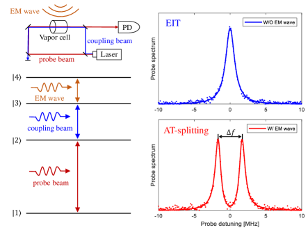
Figure 2: The EIT-AT phenomenon of a four-level system, where $\ket{3}$ and $\ket{4}$ represent the Rydberg states. For example, in literature [12], $\ket{1}$, $\ket{2}$, $\ket{3}$, and $\ket{4}$ correspond to the energy levels $6S_{1/2}$, $6P_{3/2}$, $47S_{1/2}$, and $47P_{1/2}$ for measuring $37.4065\>{\rm GHz}$ electromagnetic wave.

II-E Implementation of Atomic Receiver

Despite the elegant mathematical representation of Rabi oscillation in (5), observing this phenomenon in practice is quite challenging due to various external disturbances that can destroy the coherence of a quantum state, such as spontaneous emission [25]. Fortunately, the data-bearing effective Rabi frequency is still measurable, as it can induce two other quantum phenomena, namely electromagnetically induced transparency (EIT) and Autler-Townes (AT) splitting [5]. As shown in Fig. 2, the EIT-AT phenomenon involves a four-level system denoted by quantum states $\ket{1}$, $\ket{2}$, $\ket{3}$, and $\ket{4}$, where $\ket{3}$ and $\ket{4}$ represent the Rydberg states we studied before. Recall that when preparing a Rydberg state, two laser beams, the probe beam and coupling beam, are needed to excite the electron from $\ket{1}$ to $\ket{2}$ and then from $\ket{2}$ to $\ket{3}$. In practice, a PD is deployed to receive the probe beam and illustrate its spectrum for observing the Rabi frequency. When the incident electromagnetic wave is turned off and the probe beam is turned resonant with the transition $\ket{1}\rightarrow\ket{2}$, the EIT phenomenon occurs such that the probe beam penetrates through the vapor cell nearly without absorption loss. What reflects on its spectrum is that one peak appears at the resonant frequency (see the upper sub-figure of Fig. 2). On the other hand, when the incident electromagnetic wave is turned on, the two Rydberg states $\ket{3}$ and $\ket{4}$ are coupled by the Rabi frequency. As a result, the AT splitting phenomenon is induced, which splits the peak of the spectrum of the probe beam into two as depicted in the lower sub-figure of Fig. 2. As physicists have demonstrated, the splitting interval $\Delta f$ of the two peaks is linearly proportional to the effective Rabi frequency [7]:

$$\Delta f=\frac{\lambda_{c}}{\lambda_{p}}\frac{\Omega}{2\pi},$$ (6)

where $\lambda_{c}$ and $\lambda_{p}$ denote the wavelengths of the coupling and probe beams, respectively. Then, measuring $\Delta f$, the effective Rabi frequency, $\Omega=2\pi\frac{\lambda_{p}}{\lambda_{c}}\Delta f$, can be read out to infer the transmitted symbol.

III Overview of Atomic MIMO Receiver

In the preceding section, we introduce the principles of atomic SISO receiver. In this section, building on these principles, we propose the atomic MIMO receiver for multi-user communications. First, its architecture and principles are presented. Then, the problem of atomic-MIMO detection is formulated, which is solved in the next section.

III-A Architecture and Principles of Atomic MIMO Receiver

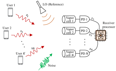
Figure 3: Schematic diagram of the atomic MIMO receiver. One atomic receiver employing $N$ atomic antennas is measuring signals from $K$-single antenna users together with one reference source, polluted by external noise.

Consider the multi-user communication system illustrated in Fig. 3, where $K$ single-antenna users communicate with one atomic MIMO receiver. Its architecture comprises $N$ vapor cells filled with Rydberg atoms and an equal number of PDs. Each vapor cell acts as an atomic antenna for measuring electromagnetic waves, while the PDs read out the measurement results (i.e., the splitting interval, $\Delta_{f}$, and the Rabi frequency, $\Omega_{R}$) and aggregate them to the digital processor for signal detection. The simultaneous users share the same carrier frequency $\omega$, while all atoms are triggered to the uniform Rydberg states $\hbar\omega_{g}$ and $\hbar\omega_{e}$ (e.g., $52D_{5/2}$ and $53P_{3/2}$) in response to the carrier frequency (e.g., $\omega=5$ GHz). As a result, the resonance case with $\omega=\omega_{eg}$ is created. The principles and operations of the receiver are described in the sequel.

Consider an arbitrary user, say the $k$-th user. Its phase modulated symbol is denoted as $s_{k}=|s_{k}|e^{i\gamma_{k}}\in\mathcal{S}$, where the quadrature amplitude modulation (QAM) is adopted and the set $\mathcal{S}$ corresponds to the QAM constellation. The average power of $s_{k}$ is normalized as $\mathsf{E}(\|s_{k}\|^{2})=1$. Then, the transmit RF signal is given as $x_{k}(t)=\sqrt{P_{k}}|s_{k}|\cos(\omega t+\gamma_{k})$. The simultaneous transmissions from all users result in the received vector-form electromagnetic wave at the $n$-th vapor cell given as

$${\mathbf{E}}_{n}(t)=\sum_{k=1}^{K}\bm{\epsilon}_{n,k}\sqrt{P_{k}}\rho_{n,k}|s_{k}|\cos(\omega t+\varphi_{n,k}+\gamma_{k}),$$ (7)

where the variables $\bm{\epsilon}_{n,k}$, $\rho_{n,k}$, and $\varphi_{n,k}$ represent the polarization, path loss, and phase shift of the propagation from the $k$-th user to the $n$-th antenna.

Next, consider an arbitrary vapor cell, say the $n$-th cell at the receiver. For each atom inside this cell, its quantum state can be expressed as $\ket{\psi(t)}_{n}=\alpha_{g,n}(t)\ket{g}+\alpha_{e,n}(t)\ket{e}=[\alpha_{e,n}(t),\alpha_{g,n}(t)]^{T}$. Similarly as in the SISO case, the evolution of $\ket{\psi(t)}_{n}$ is governed by the Schrödinger equation

$$i\hbar\frac{\partial\ket{\psi(t)}_{n}}{\partial t}=(\hat{H}_{n}+\hat{V}_{n})\ket{\psi(t)}_{n}.$$ (8)

As all atoms are exited to the uniform Rydberg states, the free Hamiltonian $\hat{H}_{n}$ is the same as that in Appendix A, i.e., $\hat{H}_{n}=\mathrm{diag}\{\hbar\omega_{e},\hbar\omega_{g}\}$. On the other hand, the interaction Hamiltonian $\hat{V}_{n}$ requires the expression of the incident wave ${\mathbf{E}}_{n}(t)$ and the position operator $\hat{{\mathbf{r}}}_{n}$. Similar to the discussion in Appendix A, the interaction Hamiltonian is given as $\hat{V}_{n}=q\hat{{\mathbf{r}}}_{n}^{T}{\mathbf{E}}_{n}(t)=\sum_{k=1}^{K}(\hat{{\mathbf{r}}}_{n}^{T}\bm{\epsilon}_{n,k})q\sqrt{P_{k}}\rho_{n,k}|s_{k}|\cos(\omega t+\varphi_{n,k}+\gamma_{k})$. Then, expanding the position operator $\hat{{\mathbf{r}}}_{n}$ on the basis $\{\ket{g},\ket{e}\}$ as $\hat{{\mathbf{r}}}_{n}=\bra{e}\hat{{\mathbf{r}}}_{n}\ket{g}(\ket{e}\bra{g}+\ket{g}\bra{e})$, we can get the matrix-form expression: $\hat{V}_{n}=\xi_{n}(t)(\ket{e}\bra{g}+\ket{g}\bra{e})$, where

$$\xi_{n}(t){=}\sum_{k=1}^{K}{{\mathbf{r}}}_{eg}^{T}\bm{\epsilon}_{n,k}q\sqrt{P_{k}}\rho_{n,k}|s_{k}|\cos(\omega t+\varphi_{n,k}+\gamma_{k}).$$ (9)

Last, substituting $\hat{H}_{n}$ and $\hat{V}_{n}$ into Schrödinger equation and applying the rotating wave approximation, we can derive the probability amplitude based on the initial state $\alpha_{e,n}(0)=0$:

$$|\alpha_{e,n}(t)|^{2}=\sin^{2}\left(\frac{\Omega_{R,n}}{2}t\right),$$ (10)

where the Rabi frequency is given as

$$\Omega_{R,n}=\left|\sum_{k=1}^{K}\frac{1}{\hbar}({{\mathbf{r}}}_{eg}^{T}\bm{\epsilon}_{n,k})q\sqrt{P_{k}}\rho_{n,k}|s_{k}|e^{i(\varphi_{n,k}+\gamma_{k})}\right|.$$ (11)

Note that the detuning factor, $\delta$, vanishes since $\delta=\omega_{eg}-\omega=0$. The preceding formula characterizes the quantum-jump behavior of the $n$-th atomic antenna as triggered by $K$ sources, where multi-user symbols, $\{s_{k}\}$, are encoded in the Rabi frequencies, $\{\Omega_{R,n}\}$.

The goal of atomic-MIMO receiver is to read the values of $\{\Omega_{R,n}\}$ and infer $\{s_{k}\}$ from $\{\Omega_{R,n}\}$. To this end, according to the principle of EIT-AT discussed in Section II-E, the Rabi frequency, $\Omega_{R,n}$, can be measured by the splitting interval, $\Delta f_{n}$, of the probe-beam spectrum since $\Omega_{R,n}=2\pi\frac{\lambda_{p}}{\lambda_{c}}\Delta f_{n}$. For ease of exposition, let the measurement of $\Omega_{R,n}$ be denoted as $z_{n}$, which is the equivalent received signal at the $n$-th antenna. To facilitate the detector design, a compact matrix form of $\{z_{n}\}$ is derived as follows. We define ${\mathbf{s}}=[s_{1},s_{2},\cdots,s_{K}]^{T}$ and ${\mathbf{a}}_{n}=[a_{n,1},a_{n,2},\cdots,a_{n,K}]^{T}$, where $a_{n,k}=\frac{1}{\hbar}({{\mathbf{r}}}_{eg}^{T}\bm{\epsilon}_{n,k})q\sqrt{P_{k}}\rho_{n,k}e^{-i\varphi_{n,k}}$. It is straightforward to obtain that $z_{n}=\left|{\mathbf{a}}_{n}^{H}{\mathbf{s}}\right|$. We further define the received vector-form signal as ${\mathbf{z}}=[z_{1},z_{2},\cdots,z_{N}]^{T}$ and the observation matrix as ${\mathbf{A}}=[{\mathbf{a}}_{1},{\mathbf{a}}_{2},\cdots,{\mathbf{a}}_{N}]\in\mathbb{C}^{K\times N}$. It follows that

$${\mathbf{z}}=|{\mathbf{A}}^{H}{\mathbf{s}}|,$$ (12)

where the operator $|{\mathbf{x}}|$ takes the magnitude of each element of the vector, ${\mathbf{x}}$. A crucial conclusion is drawn from (12) that the transmit symbols in ${\mathbf{s}}$ are embedded in the observed amplitude vector ${\mathbf{z}}=|{\mathbf{A}}^{H}{\mathbf{s}}|$, where the observation matrix ${\mathbf{A}}$ can be treated as an effective MIMO channel. As opposed to the linear model adopted in conventional MIMO communications, the atomic MIMO receiver features a non-linear model based on amplitude detection. This is equivalent to the well-known PR model in the realm of optical imaging [26].

Before delving into this PR problem, two factors, which are part of the proposed framework and affecting the receiver effectiveness, are described as follows.

• Reference signal: To begin with, as shown in Fig. 3, a measurement scheme called holographic phase-sensing, where a LO sends a known reference signal, $s_{b}$, to the atomic receiver, is often employed to detect QAM symbols [15]. To be specific, as the phase information is erased in (12), the absolute phase $e^{i\angle{\mathbf{s}}}$ of ${\mathbf{s}}$ is undetectable. However, with the help of the known reference signal $s_{b}$, one can infer the absolute phase, $e^{i\angle{\mathbf{s}}}$, by estimating the phase difference between ${\mathbf{s}}$ and $s_{b}$, thereby enabling QAM detection. Let the reference signal have the same carrier frequency $\omega$. Then, following the same steps as (7) to (12), we can arrive at the modified received signal: ${\mathbf{z}}=|{\mathbf{A}}^{H}{\mathbf{s}}+{\mathbf{b}}|$, where ${\mathbf{b}}=[b_{1},b_{2},\cdots,b_{N}]^{T}$, $b_{n}=\frac{s_{b}}{\hbar}({{\mathbf{r}}}_{eg}^{T}\bm{\epsilon}_{b,n})q\sqrt{P_{b}}\rho_{b,n}e^{-i\varphi_{b,n}}$, and $P_{b}$, $\rho_{b,n}$, $\varphi_{b,n}$, and ${\mathbf{\epsilon}}_{b,n}$ represent the transmit power, path loss, phase shift, and polarization pertaining to the reference signal, respectively.

• Noise model: The noise perturbing the atomic MIMO receiver is attributed to multiple sources including internal thermal noise, photon shot noise, and external interference [7]. The aggregation of sources allow us to invoke the law-of-large-number to model the noise as an additive Gaussian random vector, ${\mathbf{w}}\sim\mathcal{CN}(0,\sigma^{2}{\mathbf{I}})$.

By adding the reference signal and noise into (12), we obtain the following input-output relationship for the atomic MIMO systems as

$${\mathbf{z}}=|{\mathbf{A}}^{H}{\mathbf{s}}+{\mathbf{b}}+{\mathbf{w}}|.$$ (13)

Due to the presence of reference signal ${\mathbf{b}}$, (13) is called a biased PR model as opposed to the typical PR model without this reference signal.

III-B Atomic-MIMO Detection Problems

The problem of atomic-MIMO detection is to estimate the multi-user data vector, ${\mathbf{s}}$, from the received signal, ${\mathbf{z}}$, in (13). Two problem formulations are provided below.

III-B1 Least-Square Criterion

The first formulation follows the typical LS criterion:

$$\min_{{\mathbf{s}}\in\mathcal{S}^{K}}\left\|{\mathbf{z}}-|{\mathbf{A}}^{H}{\mathbf{s}}+{\mathbf{b}}|\right\|_{2}^{2}.$$ (14)

III-B2 Maximum-Likelihood Criterion

It can be proven that each entry of ${\mathbf{z}}$ follows the Rician distribution, i.e.,

$$p(z_{n};{\mathbf{s}})=\frac{2z_{n}}{\sigma^{2}}\exp\left(-\frac{z_{n}^{2}+|\lambda_{n}|^{2}}{\sigma^{2}}\right)I_{0}\left(\kappa_{n}\right),$$ (15)

where $\lambda_{n}\overset{\Delta}{=}{\mathbf{a}}_{n}^{H}{\mathbf{s}}+b_{n}$, $\kappa_{n}\overset{\Delta}{=}\frac{2z_{n}|{\mathbf{a}}_{n}^{H}{\mathbf{s}}+b_{n}|}{\sigma^{2}}$, and $I_{0}(x)=\frac{1}{2\pi}\int_{0}^{2\pi}e^{x\cos\theta}\text{d}\theta$ is the modified zero-order Bessel function. Thereby, for any given realization of the effective channel and reference, the ML detection of ${\mathbf{s}}$ is formulated as

$$\max_{{\mathbf{s}}\in\mathcal{S}^{K}}\sum_{n=1}^{N}\log p(z_{n};{\mathbf{s}})\propto\sum_{n=1}^{N}-\frac{|\lambda_{n}|^{2}}{\sigma^{2}}+\log I_{0}\left(\kappa_{n}\right).$$ (16)

Although problems (14) and (16) can be optimally solved by an exhaustive search, the complexity is prohibitive when the users are many and/or the constellation size is large. To this end, two low-complexity algorithms are designed in the next section.

IV Atomic-MIMO Detection Algorithms

In this section, we present two atomic-MIMO detection algorithms to solve the biased PR problems formulated in the preceding section. Their performance and complexity are subsequently analyzed.

IV-A LS Phase Retrieval Algorithm

Consider the biased PR problem in (14) corresponding to LS detection. One of the most popular PR solvers is the Gerchberg-Saxton (GS) algorithm [22]. We transform the classical GS algorithm to a biased GS algorithm to solve the biased PR problem in (14) . The result is summarized in Algorithm 1 and elaborated as follows.

Define ${\mathbf{y}}=[y_{1},y_{2},\cdots,y_{N}]^{T}={\mathbf{A}}^{H}{\mathbf{s}}+{\mathbf{b}}+{\mathbf{w}}$. The fundamental idea of the GS algorithm is that if the true phase $e^{i\bm{\theta}}$ of ${\mathbf{y}}$ is accessible, where $e^{i\bm{\theta}}=[e^{i\angle{y_{1}}},e^{i\angle{y_{2}}},\cdots,e^{i\angle{y_{N}}}]^{T}$, then problem (14) becomes a linear regression problem: $\min_{{\mathbf{s}}}\|{\mathbf{z}}\circ e^{i\bm{\theta}}-{\mathbf{A}}^{H}{\mathbf{s}}-{\mathbf{b}}\|$, whose solution is ${\mathbf{s}}=({\mathbf{A}}{\mathbf{A}}^{H})^{-1}{\mathbf{A}}({\mathbf{z}}\circ e^{i\bm{\theta}}-{\mathbf{b}})$, where $\circ$ denotes the Hadamard product. As the knowledge on $e^{i\bm{\theta}}$ is unavailable, an alternative approach is to jointly optimize $e^{i\bm{\theta}}$ and ${\mathbf{s}}$:

$$\min_{\bm{\theta},{\mathbf{s}}\in\mathcal{S}^{K}}\left\|{\mathbf{z}}\circ e^{i\bm{\theta}}-{\mathbf{A}}^{H}{\mathbf{s}}-{\mathbf{b}}\right\|_{2}^{2}.$$ (17)

Problem (17) is non-convex since $e^{i\bm{\theta}}$ is an oscillating function with respect to (w.r.t) $\bm{\theta}$. Fortunately, this optimization problem can be efficiently solved by the well-known alternating minimization methodology. To be specific, $\bm{\theta}$ and ${\mathbf{s}}$ are iteratively updated as presented in Steps 6-7 of Algorithm 1. During the $t$-th iteration, given the previous estimate ${\mathbf{s}}^{t-1}$, $\bm{\theta}$ can be optimized by extracting the phase of ${\mathbf{A}}^{H}{\mathbf{s}}^{t-1}+{\mathbf{b}}$, that is $\bm{\theta}^{t}=\angle({\mathbf{A}}^{H}{\mathbf{s}}^{t-1}+{\mathbf{b}})$. Furthermore, given $\bm{\theta}^{t}$, the optimal ${\mathbf{s}}$ is determined by the LS rule: ${\mathbf{s}}^{t}=({\mathbf{A}}{\mathbf{A}}^{H})^{-1}{\mathbf{A}}({\mathbf{z}}\circ e^{i\bm{\theta}^{t}}-{\mathbf{b}})$.

Algorithm 1 : Biased GS Algorithm

0:    The equivalent received signal ${\mathbf{z}}$, the equivalent channel matrix ${\mathbf{A}}$, the reference field ${\mathbf{b}}$, the total number of iterations $t_{0}$.

1:  Construct the augmented observation matrix $\bar{{\mathbf{A}}}=[{\mathbf{A}}^{H},{\mathbf{b}}]^{H}=[\bar{{\mathbf{a}}}_{1},\bar{{\mathbf{a}}}_{2},\cdots\bar{{\mathbf{a}}}_{N}]$

2:  Find the principal eigenvector ${\mathbf{v}}$ of ${\mathbf{M}}=\sum_{n=1}^{N}z_{n}\bar{{\mathbf{a}}}_{n}\bar{{\mathbf{a}}}_{n}^{H}$

3:  Set $\bar{r}=\frac{|{\mathbf{v}}^{H}\bar{{\mathbf{A}}}|{\mathbf{z}}}{\|\bar{{\mathbf{A}}}^{H}{\mathbf{v}}\|_{2}^{2}}$ and $\bar{{\mathbf{s}}}^{0}=\bar{r}{\mathbf{v}}$

4:  Initialize ${\mathbf{s}}^{0}=e^{-i\angle\bar{{\mathbf{s}}}^{0}(K+1)}\bar{{\mathbf{s}}}^{0}(1:K)$

5:  for $t=\{1,2,\cdots,t_{0}\}$ do

6:     Update $\bm{\theta}^{t}=\angle({\mathbf{A}}^{H}{\mathbf{s}}^{t-1}+{\mathbf{b}})$

7:     Update ${\mathbf{s}}^{t}=({\mathbf{A}}{\mathbf{A}}^{H})^{-1}{\mathbf{A}}({\mathbf{z}}\circ e^{i\bm{\theta}^{t}}-{\mathbf{b}})$

8:  end for

8:    The estimated symbol $\tilde{{\mathbf{s}}}={\mathbf{s}}^{t_{0}}$

One issue in the implementation of the biased GS algorithm is its sensitivity to the choice of initial point. Without a proper initial estimate, Algorithm 1 may converge to an undesirable local optimum. To address this issue, the computationally efficient spectral method has been developed to yield good initialization [27]. Specifically, to adopt the spectral method into our model, we first construct an augmented observation matrix $\bar{{\mathbf{A}}}=[{\mathbf{A}}^{H},{\mathbf{b}}]^{H}$ as presented in Step 1. This matrix allows us to treat the user signal and reference signal together: $\bar{{\mathbf{s}}}=[{\mathbf{s}}^{H},1]^{H}$. Thereafter the observed amplitude vector can be rewritten in a reference-free form: ${\mathbf{z}}=|{\mathbf{A}}^{H}{\mathbf{s}}+{\mathbf{b}}+{\mathbf{w}}|=|\bar{{\mathbf{A}}}^{H}\bar{{\mathbf{s}}}+{\mathbf{w}}|$, whose initialization can be performed using the typical spectral method. To elaborate, define the weighted covariance matrix as ${\mathbf{M}}=\sum_{n=1}^{N}z_{n}\bar{{\mathbf{a}}}_{n}\bar{{\mathbf{a}}}_{n}^{H}$, where $\bar{{\mathbf{a}}}_{n}$ denotes the $n$-th column of $\bar{{\mathbf{A}}}$. The direction of the initial value $\bar{{\mathbf{s}}}^{0}$ of $\bar{{\mathbf{s}}}$ is estimated as the principal eigenvector ${\mathbf{v}}$ of ${\mathbf{M}}$. In addition, the magnitude $\bar{r}$ of $\bar{{\mathbf{s}}}^{0}$ is obtained by approaching $|{\mathbf{A}}^{H}\bar{{\mathbf{s}}}^{0}|=|{\mathbf{A}}^{H}\bar{r}{\mathbf{v}}|$ to ${\mathbf{z}}$:

$$\bar{r}=\arg\min_{r^{\prime}}\|{r^{\prime}}|{\mathbf{A}}^{H}{\mathbf{v}}|-{\mathbf{z}}\|_{2}^{2}=\frac{|{\mathbf{v}}^{H}\bar{{\mathbf{A}}}|{\mathbf{z}}}{\|\bar{{\mathbf{A}}}^{H}{\mathbf{v}}\|_{2}^{2}}.$$ (18)

Thereafter, $\bar{{\mathbf{s}}}$ is initialized as $\bar{{\mathbf{s}}}^{0}=\bar{r}{\mathbf{v}}$. Recall that only the first $K$ entries of $\bar{{\mathbf{s}}}$ are the wanted symbols from users, while the last entry of $\bar{{\mathbf{s}}}$ refers to the known value 1 with a zero phase. Hence, ${\mathbf{s}}^{0}$ is initialized by forcing the phase of the last entry of $\bar{{\mathbf{s}}}^{0}$ to zero:

$${\mathbf{s}}^{0}=e^{-i\angle\bar{{\mathbf{s}}}^{0}(K+1)}\bar{{\mathbf{s}}}^{0}(1:K),$$ (19)

which completes the initialization. After carrying out the initialization and $t_{0}$-step iterations, the final estimate is obtained as $\tilde{{\mathbf{s}}}={\mathbf{s}}^{t_{0}}$. Last, one can project each entry of $\tilde{{\mathbf{s}}}$ to the nearest point of the QAM constellation to perform demapping, i.e., $\hat{s}_{k}=\arg\min_{s\in\mathcal{S}}\|\tilde{s}_{k}-s\|$.

The main limitation of the LS based biased GS algorithm arises as it fails to consider the distribution of the received signal, leaving margin for performance improvement. The limitation can be overcome by the ML algorithm in the sequel.

Algorithm 2 : EM-GS Algorithm

0:    The equivalent received signal ${\mathbf{z}}$, the equivalent channel matrix ${\mathbf{A}}$, the reference field ${\mathbf{b}}$, the power density of noise $\sigma$, the number of iterations $t_{0}$.

1:  Construct the augmented observation matrix $\bar{{\mathbf{A}}}=[{\mathbf{A}}^{H},{\mathbf{b}}]^{H}=[\bar{{\mathbf{a}}}_{1},\bar{{\mathbf{a}}}_{2},\cdots\bar{{\mathbf{a}}}_{N}]$

2:  Find the principal eigenvector ${\mathbf{v}}$ of ${\mathbf{M}}=\sum_{n=1}^{N}z_{n}\bar{{\mathbf{a}}}_{n}\bar{{\mathbf{a}}}_{n}^{H}$

3:  Set $\bar{r}=\frac{|{\mathbf{v}}^{H}\bar{{\mathbf{A}}}|{\mathbf{z}}}{\|\bar{{\mathbf{A}}}^{H}{\mathbf{v}}\|_{2}^{2}}$ and $\bar{{\mathbf{s}}}^{0}=\bar{r}{\mathbf{v}}$

4:  Initialize ${\mathbf{s}}^{0}=e^{-i\angle\bar{{\mathbf{s}}}^{0}(K+1)}\bar{{\mathbf{s}}}^{0}(1:K)$

5:  for $t=\{1,2,\cdots,t_{0}\}$ do

6:     Update $\bm{\theta}^{t}=\angle({\mathbf{A}}^{H}{\mathbf{s}}^{t-1}+{\mathbf{b}})$

7:     Update $\bm{\kappa}^{t}=\frac{2}{\sigma^{2}}{\mathbf{z}}\circ|{\mathbf{A}}^{H}{\mathbf{s}}^{t-1}+{\mathbf{b}}|$

8:     Update ${\mathbf{s}}^{t}=({\mathbf{A}}{\mathbf{A}}^{H})^{-1}{\mathbf{A}}({\mathbf{z}}\circ e^{i\bm{\theta}^{t}}\circ R(\bm{\kappa}^{t})-{\mathbf{b}})$

9:  end for

9:    The estimate symbol $\tilde{{\mathbf{s}}}={\mathbf{s}}^{t_{0}}$

IV-B ML Phase Retrieval Algorithm

Consider the ML detection problem in (16). We propose to solve it by integrating the Expectation-Maximization (EM) and aforementioned GS algorithm, termed the EM-GS algorithm. One can observe from (16) that the occurrence of the non-trivial modified Bessel function $I_{0}(\cdot)$ makes the ML detection intractable. To overcome this difficulty, the EM method is employed to create a series of tractable lower-bound surrogate functions to the primal objective in (16), resulting in sequentially updated estimates of ${\mathbf{s}}^{t}$ for $t=1,2,\cdots,t_{0}$ as summarized in Algorithm 2. The detailed EM-GS algorithm is designed as follows.

To begin with, recall the definition ${\mathbf{y}}={\mathbf{A}}^{H}{\mathbf{s}}+{\mathbf{b}}+{\mathbf{w}}={\mathbf{z}}\circ e^{i\bm{\theta}}$. Like the basic idea of the biased GS algorithm, the phase $e^{i\bm{\theta}}$ is an unobserved but crucial variable, the information of which can substantially simplify our problem. This observation motivates us to treat the phase $e^{i\bm{\theta}}$ as a latent variable in our EM algorithm. Based on the Jensen inequality, the EM algorithm states that the loglikelihood function is lower-bounded by the following surrogate function:

$$\sum_{n=1}^{N}\log p(z_{n};{\mathbf{s}}) \geq\sum_{n=1}^{N}\mathsf{E}_{p(\theta_{n}|z_{n},{\mathbf{s}}^{t-1})}\log p(z_{n},\theta_{n};{\mathbf{s}})$$

$$\overset{\Delta}{=}Q({\mathbf{s}}|{\mathbf{s}}^{t-1}),$$ (20)

where ${\mathbf{s}}^{t-1}$ denotes the previous estimate of ${\mathbf{s}}$. The EM algorithm proceeds iteratively by two steps to maximize the loglikelihood. They are the Expectation step (E-step) to derive the surrogate function $Q({\mathbf{s}}|{\mathbf{s}}^{t-1})$ by calculating the expectation in (IV-B), and the Maximization step (M-step) to update ${\mathbf{s}}^{t}$ by maximizing $Q({\mathbf{s}}|{\mathbf{s}}^{t-1})$, i.e., ${\mathbf{s}}^{t}=\arg\max_{{\mathbf{s}}}Q({\mathbf{s}}|{\mathbf{s}}^{t-1})$. These two steps are elaborated below.

• E-step: In (IV-B), the likelihood function $p(z_{n},\theta_{n};{\mathbf{s}})$ stands for the ML estimator to ${\mathbf{s}}$ when both the amplitude $z_{n}$ and phase $\theta_{n}$ are accessible. Clearly, $p(z_{n},\theta_{n};{\mathbf{s}})$ is a Gaussian distribution

  $$p(z_{n},\theta_{n};{\mathbf{s}}) =\frac{1}{\pi\sigma^{2}}\exp\left(-\frac{1}{\sigma^{2}}\left|z_{n}e^{i\theta_{n}}-\lambda_{n}\right|\right),$$ (21)

  where $\lambda_{n}\overset{\Delta}{=}{\mathbf{a}}_{n}^{H}{\mathbf{s}}+b_{n}$. As for the posterior probability $p(\theta_{n}|z_{n},{\mathbf{s}}^{t-1})$, it refers to our current knowledge to the phase $\theta_{n}$ given previous estimate ${\mathbf{s}}^{t-1}$. As shown in [28], $p(\theta_{n}|z_{n},{\mathbf{s}}^{t-1})$ follows the von Mises distribution:

  $$p(\theta_{n}|z_{n},{\mathbf{s}}^{t-1})=\frac{\exp\left(\kappa_{n}^{t}\cos(\theta_{n}-\theta_{n}^{t})\right)}{2\pi I_{0}(\kappa_{n}^{t})},$$ (22)

  where $\theta_{n}^{t}\overset{\Delta}{=}\angle\left({\mathbf{a}}_{n}^{H}{\mathbf{s}}^{t-1}+b_{n}\right)$ and $\kappa_{n}^{t}\overset{\Delta}{=}\frac{2z_{n}|{\mathbf{a}}_{n}^{H}{\mathbf{s}}^{t-1}+b_{n}|}{\sigma^{2}}$. Based on (21) and (22), we derive the following result that defines the E-step.

  Lemma 1.

  The surrogate function is expressed as

  $$Q({\mathbf{s}}|{\mathbf{s}}^{t-1})=-\frac{1}{\sigma^{2}}\|{\mathbf{z}}\circ e^{i\bm{\theta}^{t}}\circ R(\bm{\kappa}^{t})-{\mathbf{A}}^{H}{\mathbf{s}}-{\mathbf{b}}\|_{2}^{2}+C,$$ (23)

  where $e^{i\bm{\theta}^{t}}=[e^{i\theta_{1}^{t}},e^{i\theta_{2}^{t}},\cdots,e^{i\theta_{N}^{t}}]^{T}=e^{i\angle({\mathbf{A}}^{H}{\mathbf{s}}^{t-1}+{\mathbf{b}})}$, $\bm{\kappa}^{t}=[\kappa_{1}^{t},\kappa_{2}^{t},\cdots,\kappa_{N}^{t}]^{T}=\frac{2}{\sigma^{2}}{\mathbf{z}}\circ|{\mathbf{A}}^{H}{\mathbf{s}}^{t-1}+{\mathbf{b}}|$, $R(x)\overset{\Delta}{=}\frac{I_{1}(x)}{I_{0}(x)}$, $I_{1}(x)$ represents the first-order modified Bessel function, and $C$ denotes a constant irrelevant to ${\mathbf{s}}$.

  Proof: (See Appendix B).  $\Box$

M-step: Lemma 1 reveals that the maximization of $Q({\mathbf{s}}|{\mathbf{s}}^{t-1})$ is equivalent to the minimization of $\|{\mathbf{z}}\circ e^{i\bm{\theta}^{t}}\circ R(\bm{\kappa}^{t})-{\mathbf{A}}^{H}{\mathbf{s}}-{\mathbf{b}}\|_{2}^{2}$. In this context, the primal non-convex optimization problem in (16) is converted to a sequence of easily handled linear regression problems. Therefore, as presented in Steps 6-8 of Algorithm 2, the estimate of ${\mathbf{s}}$ is updated successively by

$${\mathbf{s}}^{t}=({\mathbf{A}}{\mathbf{A}}^{H})^{-1}{\mathbf{A}}({\mathbf{z}}\circ e^{i\bm{\theta}^{t}}\circ R(\bm{\kappa}^{t})-{\mathbf{b}}),$$ (24)

where the final estimate is given as $\tilde{{\mathbf{s}}}={\mathbf{s}}^{t_{0}}$.

Moreover, to avoid convergence to a poor local optimum, the spectral method based on the augmented matrix $\bar{{\mathbf{A}}}$ as used in Section IV-A is carried out to obtain an initial estimate ${\mathbf{s}}^{0}$. In the end, after performing the initialization and EM-based iteration, the projection operation $\hat{s}_{k}=\arg\min_{s\in\mathcal{S}}\|\tilde{s}_{k}-s\|$ is applied to complete the constellation demapping.

IV-C Comparison between biased GS and EM-GS algorithms

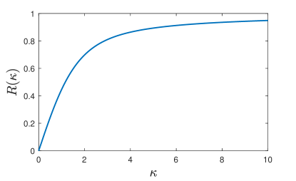
Figure 4: The high-pass filter corresponding to $R(\kappa)$ for $\kappa\in[0,10]$.

Comparing Algorithms 1 and 2, one can discover that the major difference between the proposed EM-GS and biased GS is attributed to the ratio of Bessel functions, $R(\kappa_{n}^{t})=\frac{I_{1}(\kappa_{n}^{t})}{I_{0}(\kappa_{n}^{t})}$. According to the properties of Bessel functions [29], $R(\kappa_{n}^{t})$ is monotonically increasing and bounded between $[0,1]$. As plotted in Fig. 4, the shape of $R(\kappa_{n}^{t})$ resembles that of a high-pass filter. Note that the variable $\kappa_{n}^{t}=\frac{2z_{n}|{\mathbf{a}}_{n}^{H}{\mathbf{s}}^{t-1}+b_{n}|}{\sigma^{2}}$ implicitly represents the SNR at the $n$-th antenna. A stronger received signal energy $z_{n}|{\mathbf{a}}_{n}^{H}{\mathbf{s}}^{t-1}+b_{n}|$ together with a smaller noise power $\sigma^{2}$ leads to a larger value of $\kappa_{n}^{t}$. Therefore, by multiplying $z_{n}$ with $R(\kappa_{n}^{t})$, we can filter out the received signals $z_{n}$ that have a low SNR, while keeping those $z_{n}$ that have a large SNR and contain useful information about the symbol ${\mathbf{s}}$. Consequently, the high-pass nature of $R(\kappa_{n}^{t})$ ensures that the EM-GS outperforms biased GS in the low SNR regime, while the EM-GS will automatically degenerate to biased GS at high SNRs, where $R(\kappa_{n}^{t})\rightarrow 1$ when $\kappa_{n}^{t}\rightarrow+\infty$. Simulation results are provided in Section IV to quantitatively compare the performance of biased GS and EM-GS algorithms.

IV-D Performance Analysis

IV-D1 CRLB Analysis

We now derive the CRLB for evaluating the accuracy of the detected $\tilde{{\mathbf{s}}}$ from Algorithms 1 and 2. CRLB provides a lower bound of $\mathsf{E}(\|{\mathbf{s}}-\tilde{{\mathbf{s}}}\|_{2}^{2})$ for any unbiased estimate. Specifically, the CRLB of the distribution $p({\mathbf{z}};{\mathbf{s}})=\prod_{n=1}^{N}p(z_{n};{\mathbf{s}})$ is expressed as

$${\mathbf{C}}_{{\mathbf{s}}}=\mathsf{E}({\mathbf{s}}-\tilde{{\mathbf{s}}})({\mathbf{s}}-\tilde{{\mathbf{s}}})^{H}\geq{\mathbf{I}}^{-1},$$ (25)

where ${\mathbf{I}}$ denotes the Fisher information matrix, the $(p,q)$-th entry of which is determined by $I_{pq}=-\sum_{n=1}^{N}\mathsf{E}\left(\frac{\partial^{2}}{\partial s_{p}^{*}\partial s_{q}}\log p(z_{n};{\mathbf{s}})\right)$. An explicit expression of ${\mathbf{I}}$ is provided by the following Lemma 2.

Lemma 2.

The Fisher Information matrix for the Rician distribution (15) is given by

$${\mathbf{I}}=\sum_{n=1}^{N}\beta_{n}{\mathbf{a}}_{n}{\mathbf{a}}_{n}^{H},$$ (26)

where $\beta_{n}=\frac{1}{\sigma^{4}}(\mathsf{E}\{z_{n}^{2}R^{2}(\kappa_{n})\}-|\lambda_{n}|^{2})$.

Proof: (See Appendix C).  $\Box$

As a result, the mean square error $\mathsf{E}(\|{\mathbf{s}}-\tilde{{\mathbf{s}}}\|_{2}^{2})$ is lower bounded by $\mathsf{Tr}({\mathbf{I}}^{-1})$, where $\mathsf{Tr}(\cdot)$ denotes the trace operator. In Section V, we numerically show that our proposed algorithms can approach the above CRLB.

IV-D2 Computational Complexity Analysis

It is of interest to compare the computational complexity of the biased GS, EM-GS, and exhaustive search algorithms. Compared to the biased GS algorithm, the EM-GS algorithm only needs the additional computing of $R(\kappa_{n}^{t})$, which can efficiently rely on searching over a lookup table. Hence, these two algorithms share the same order of complexity. Take the EM-GS algorithm as an example. Its complexity is mainly attributed to the initialization and iteration operations. The former requires the eigenvalue decomposition of ${\mathbf{M}}\in\mathbb{C}^{K\times K}$, which has a complexity of $\mathcal{O}(K^{3})$. Moreover, the complexity of solving the linear regression problem in (23) with $t_{0}$ iterations is given as $\mathcal{O}(t_{0}NK^{2})$. As a result, the computational complexity of both the biased GS and EM-GS algorithms is $\mathcal{O}(t_{0}NK^{2}+K^{3})$.

The exhaustive search method has to try all possible symbol combinations for all users from the QAM constellation, $\mathcal{S}$, to optimize (14) and (16). Since the number of combinations is $|\mathcal{S}|^{K}$, the complexity of exhaustive search is $\mathcal{O}(|\mathcal{S}|^{K}NK)$. It is clear that the biased GS and EM-GS algorithms have much lower computational complexity than an exhaustive search.

V Simulation Results

V-A Experimental Settings

The default simulation setups for atomic MIMO receivers are as follows unless specified otherwise. The number of atomic antennas is $N=36$, while the number of single-antenna users is $K=3$. The 4-QAM and 16-QAM modulators are considered. The Rydberg energy levels $52D_{5/2}$ and $53P_{3/2}$ are adopted for detecting the sub-6G signals of frequency $\omega_{eg}=2\pi\times 5$ GHz. Then, the dipole matrix element, i.e., ${\mathbf{r}}_{eg}^{T}\bm{\epsilon}_{n,k}$ in (9), is derived according to the analytical result in [8] as follows. The position operator defined in Appendix A can be rewritten as $\hat{{\mathbf{r}}}=\hat{r}\hat{{\mathbf{u}}}$, where $\hat{r}$ and $\hat{{\mathbf{u}}}$ denote the radial and angular operators [23]. It can be proven that ${\mathbf{r}}_{eg}^{T}\bm{\epsilon}_{n,k}=\bra{e}\hat{{\mathbf{r}}}\ket{g}^{T}\bm{\epsilon}_{n,k}$ is equal to the product of the radial matrix element $r_{eg}=\bra{e}\hat{r}\ket{g}$ and the angular matrix element ${\mathbf{u}}_{eg}^{T}\bm{\epsilon}_{n,k}=\bra{e}\hat{{\mathbf{u}}}\ket{g}^{T}\bm{\epsilon}_{n,k}$ [23], i.e., ${\mathbf{r}}_{eg}^{T}\bm{\epsilon}_{n,k}=r_{eg}{\mathbf{u}}_{eg}^{T}\bm{\epsilon}_{n,k}$. As suggested in [8], $r_{eg}$ is of the order $(0.5\sim 1.5)n^{2}a_{0}$, where $a_{0}=5.292\times 10^{-11}$ m specifies the Bohr radius and $n$ is 52 in our configuration. Thus, the radial matrix element is set as $r_{eg}=52^{2}a_{0}$. Next, since the incident electromagnetic wave has a random polarization direction $\bm{\epsilon}_{n,k}$, we use a Gaussian distribution $\mathcal{N}\left(0,\frac{1}{3}\right)$ to generate the angular matrix element ${\mathbf{u}}_{eg}^{T}\bm{\epsilon}_{n,k}$. In addition, the channel coefficients $\rho_{n,k}e^{\varphi_{n,k}}$ and $\rho_{n,b}e^{\varphi_{n,b}}$ of the incident electromagnetic waves are sampled from complex Gaussian distributions $\mathcal{CN}\left(0,\frac{q^{2}}{\epsilon_{0}^{2}\lambda^{2}r_{u}^{2}}\right)$ and $\mathcal{CN}\left(0,\frac{q^{2}}{\epsilon_{0}^{2}\lambda^{2}r_{b}^{2}}\right)$, respectively, to simulate the electromagnetic field of a dipole antenna source and the small-scale fading of wireless channels. Here, $\lambda=\frac{2\pi c}{\omega}$ is the wavelength, $\epsilon_{0}$ the permittivity, $r_{u}$ the user-to-atomic receiver distance, and $r_{b}$ the LO-to-atomic receiver distance. Furthermore, we assume the transmit power is uniform for all users and fixed as $P_{k}=\frac{1}{K}P_{u}$, with $P_{u}$ being the total transmit power. Accordingly, the received SNR is given as

$${\rm SNR}=\frac{\sum_{k=1}^{K}\mathsf{E}(|a_{nk}s_{k}|^{2})}{\sigma^{2}}=\frac{q^{4}n^{4}a_{0}^{2}P_{u}}{3\hbar^{2}\epsilon_{0}^{2}\lambda^{2}r_{u}^{2}\sigma^{2}}.$$ (27)

Moreover, we define the reference-to-signal ratio (RSR) as

$${\rm RSR}=\frac{\mathsf{E}(|b_{n}|^{2})}{\mathsf{E}(|a_{nk}s_{k}|^{2})}=\frac{KP_{b}r_{u}^{2}}{P_{u}r_{b}^{2}},$$ (28)

which accounts for the relative intensity of the reference source. In our simulations, we set the power of the reference source as $P_{b}=\frac{1}{K}P_{u}$ and control the ratios $\frac{P_{u}}{r_{u}^{2}\sigma^{2}}$ and $\frac{r_{u}^{2}}{r_{b}^{2}}$ to vary SNR from $-5\>{\rm dB}$ to $12\>{\rm dB}$ and RSR from $0\>{\rm dB}$ to $25\>{\rm dB}$. The number of iterations $t_{0}$ is set as 50 for both Algorithms 1 and 2.

Five benchmarking schemes are considered in performance comparison with the proposed biased GS and EM-GS algorithms.

• ZF with known phase: Assume the ideal case where the true phase of ${\mathbf{y}}$ is known in advance. Then the zero-forcing (ZF) detector is employed to recover the data signal, ${\mathbf{s}}$.

• CRLB: We use numerical integration to calculate the normalized CRLB, $\frac{\mathsf{Tr}({\mathbf{I}}^{-1})}{\mathsf{E}(\|{\mathbf{s}}\|_{2}^{2})}=\frac{1}{K}\mathsf{Tr}({\mathbf{I}}^{-1})$. This benchmark is only used for evaluating the NMSE performance, since the normalized CRLB can be regarded as a NMSE lower bound of all PR solvers.

• Exhaustive search (LS): This method, employed for evaluating the BER, exhaustively searches all feasible constellation points to solve the LS problem in (14).

• Exhaustive search (ML): This scheme is similar to the preceding one but aims to solve the ML problem in (16).

• CM-ZF: This method is proposed to infer modulation symbols from channel magnitude (CM) in Internet-of-Things applications [30]. It utilizes an expanded linear MIMO model to approximate the PR model in (12) and addresses it via a ZF detector. We apply this scheme to our biased PR problem.

V-B Evaluation of NMSE Performance

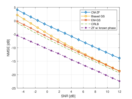
Figure 5: The dependence of NMSE performance on SNR for a 16-QAM modulator under $12\>{\rm dB}$ RSR.

Define the NMSE as $\frac{\mathsf{E}(\|{\mathbf{s}}-\tilde{{\mathbf{s}}}\|^{2}_{2})}{\mathsf{E}(\|{\mathbf{s}}\|_{2}^{2})}=\frac{1}{K}\mathsf{E}(\|{\mathbf{s}}-\tilde{{\mathbf{s}}}\|^{2}_{2})$, where $\tilde{{\mathbf{s}}}$ represents the recovered signal without constellation demapping, e.g., the direct outputs of Algorithms 1 and 2. The curves of NMSE versus SNR are plotted in Fig. 5. The RSR is fixed as $12\>{\rm dB}$ and the 16-QAM modulator is employed. It is observed from Fig. 5 that both the biased GS and the proposed EM-GS algorithms outperform the CM-ZF by $2\sim 5\>{\rm dB}$ in NMSE. Besides, the proposed EM-GS algorithm is always better than the biased GS algorithm, especially in the low SNR regime, e.g., the performance gap is around 2 dB when ${\rm SNR}=-4\>{\rm dB}$. This observation is consistent with the high-pass nature of the function $R(\cdot)$ we analyzed earlier. More importantly, the NMSE performance of EM-GS is close to CRLB, given that the ML estimator is an asymptotic minimum-variance unbiased estimator. The final interesting observation is that the NMSE gap between the ZF with known phase and CRLB approaches $3$ dB as the SNR increases, implying that the vanished phase information imposes a $3$ dB NMSE loss to atomic receivers.

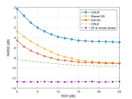
Figure 6: The effect of RSR on the NMSE performance for a 16-QAM modulator under $3\>{\rm dB}$ SNR.

We then investigate the effect of RSR on NMSE as shown in Fig. 6, where the SNR is fixed as $3$ dB and the 16-QAM modulator is adopted. As opposed to a uniform NMSE performance achieved by the ZF with known phase, the NMSE of all PR solvers rapidly declines by $5$ dB as the RSR increases. This result is surprising but still reasonable because the atomic MIMO receiver follows a non-linear model (13). A stronger reference signal makes it easier for PR solvers to estimate the phase difference between ${\mathbf{s}}$ and $s_{b}$, giving rise to a more accurate detection of the true phase of ${\mathbf{s}}$. Furthermore, the large RSR situation is common in practice because a LO can be deployed near the atomic receiver. Taking account of the path loss that decays quadratically with the path length, the strength of the reference signal can be several times greater than the user signal. For example, if the LO-to-atomic receiver distance $r_{b}$ is shorter than a quarter of the user-to-atomic receiver distance $r_{u}$, the RSR is greater than $10\log_{10}4^{2}\approx 12$ dB.

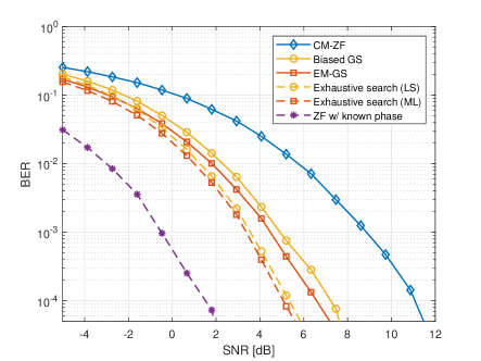
(a) 4-QAM, $N\times K=36\times 3$

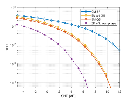
(b) 16-QAM, $N\times K=100\times 6$

Figure 7: The effect of SNR on the BER performance under (a) the small-scale configuration (i.e., $N\times K=36\times 3$, 4-QAM modulator) and (b) the large-scale configuration (i.e., $N\times K=100\times 6$, 16-QAM modulator).

V-C Evaluation of BER Performance

To evaluate the BER performance, the constellation demapping step is introduced to project the recovered signals $\tilde{s}_{k}$ for each user to the nearest constellation point $\hat{s}_{k}$ and then to 0-1 bits. The curves of BER versus SNR are plotted in Fig. 7. The RSR is set as $12$ dB. Fig. 7(a) adopts a small-scale configuration: $N\times K=36\times 3$ with a 4-QAM modulator, while Fig. (b) employs a large-scale configuration: $N\times K=100\times 6$ with a 16-QAM modulator. It can be seen from Fig. 7(a) that the biased GS and the EM-GS algorithms exhibit a remarkable BER reduction compared with CM-ZF and can perform similarly as the exhaustive search method with much lower complexity. Furthermore, the EM-GS algorithm consistently outperforms the biased GS algorithm due to the high-pass filter $R(\cdot)$ (see their comparison in Section IV-C). For the large-scale configuration depicted in Fig. 7(b), the computation of exhaustive search method is prohibitive, so it is excluded from this comparison. We can observe that the SNR gap between the EM-GS algorithm and the ZF method with known phase for realizing the same BER level is between $3\sim 4$ dB. This fact indicates that despite the lack of phase information, our EM-GS based detector can attain a similar BER trend as the ZF detector in the ideal case, demonstrating the effectiveness of multi-user atomic-MIMO detection.

Finally, the influence of RSR on BER performance is illustrated in Fig. 8. The SNR is fixed as $3$ dB and a 4-QAM modulator is adopted. Similar to Fig. 6, one can observe that the increase in RSR can considerably reduce the BER of all PR solvers. Take the proposed EM-GS as an example. More than one order of magnitude reduction in BER is achievable by increasing the RSR from $0$ dB to $20$ dB. Therefore, we can draw the conclusion that a strong received reference signal is necessary for detecting QAM symbols by atomic receivers.

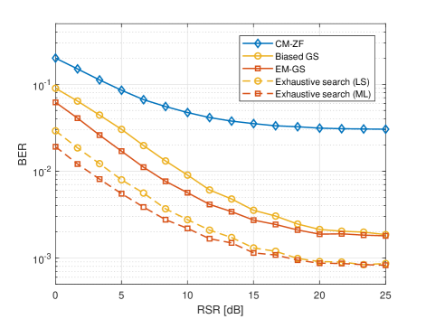
Figure 8: The effect of RSR on the BER performance under different detection algorithms for a 16-QAM modulator under $3\>{\rm dB}$ SNR.

VI Conclusions

In this paper, we have demonstrated the feasibility of atomic MIMO receivers, marking the first attempt to introduce atomic receivers into MIMO communications. Different from the classical linear MIMO model, the signal detection of atomic MIMO receiver is shown to be a non-linear biased PR problem. Accordingly, two algorithms, the biased GS and the EM-GS, are proposed to detect symbols based on the LS and ML criteria, respectively, which are verified to be near-optimal. Comprehensive experiment results validate the efficiency and effectiveness of atomic MIMO receiver.

This work serves as an important step towards advanced atomic wireless receivers for next-generation communication systems. Several unexplained issues warrant follow-up studies, such as theoretically determining the channel capacity of atomic receivers, given that the transmission model is no longer linear and Gaussian. Furthermore, integrating atomic receivers with various modern communication techniques, such as wideband, cell-free, mmWave/THz, and RIS-aided communications, and developing such receivers to enable over-the-air computation, edge learning, and ISAC, are also of interest for 6G research. Furthermore, exploring the potential incorporation of more quantum information technologies into atomic receivers to achieve unprecedented communication capabilities presents a promising research direction. As a preliminary study, this work is expected to inspire more innovations in the development of atomic receivers for advancing wireless communications.

-A Hamiltonian Operators

-A1 Free Hamiltonian

The free Hamiltonian $\hat{H}$ represents the energy of the isolated nucleus-electron system. By acting $\hat{H}$ on the ground state $\ket{g}$ and the excited state $\ket{e}$, we can obtain their energy levels $E_{g}=\hbar\omega_{g}$ and $E_{e}=\hbar\omega_{e}$, respectively. In this context, the free Hamiltonian $\hat{H}$ is expressed by a $2\times 2$ diagonal matrix as follows:

$$\hat{H}=\hbar\omega_{e}\ket{e}\bra{e}+\hbar\omega_{g}\ket{g}\bra{g}=\mathrm{diag}\{\hbar\omega_{e},\hbar\omega_{g}\}.$$ (29)

-A2 Interaction Hamiltonian

The interaction Hamiltonian $\hat{V}$ accounts for the interaction energy of the incident electromagnetic field (2) acting on this two-level system. Using Rutherford–Bohr model, we define the relative position from the nucleus to the electron as ${\mathbf{r}}=r{\mathbf{u}}$, with $r$ the length of ${\mathbf{r}}$ and ${\mathbf{u}}$ the direction of ${\mathbf{r}}$. Then, the interaction energy in classical physics is determined by $V=q{\mathbf{r}}^{T}{\mathbf{E}}(t)$, where $q$ is the charge of an electron and $q{\mathbf{r}}$ is referred to the electric dipole moment. In quantum physics, the position vector ${\mathbf{r}}$ is transformed to a position operator $\hat{{\mathbf{r}}}=[\hat{r}_{x},\hat{r}_{y},\hat{r}_{z}]^{T}$. Each entry of $\hat{{\mathbf{r}}}$ refers to a quantum operator denoted by a $2\times 2$ Hermitian matrix. According to the selection role of electron transition [25], the expansion of $\hat{r}_{d}$, $d\in\{x,y,z\}$ on the basis $\{\ket{e},\ket{g}\}$ is expressed as $\hat{r}_{d}=\bra{e}\hat{r}_{d}\ket{g}(\ket{e}\bra{g}+\ket{g}\bra{e})$, where $\bra{e}\hat{r}_{d}\ket{g}$ is a real-value number. Last, given the position operator $\hat{{\mathbf{r}}}$, the interaction Hamiltonian $\hat{V}=q\hat{{\mathbf{r}}}^{T}{\mathbf{E}}(t)$ is transferred from the interaction energy $V=q{\mathbf{r}}^{T}{\mathbf{E}}(t)$ as

$$\hat{V}=q\sum_{d\in\{x,y,z\}}\hat{r}_{d}E_{d}(t)=\left(\begin{array}[]{cc}0&\xi(t)\\ \xi(t)&0\end{array}\right),$$ (32)

where $\xi(t)\overset{\Delta}{=}({\mathbf{r}}_{eg}^{T}\bm{\epsilon})q\sqrt{P}\rho s\cos(\omega t+\varphi)$ and ${\mathbf{r}}_{eg}=\bra{e}\hat{{\mathbf{r}}}\ket{g}=[\bra{e}\hat{r}_{x}\ket{g},\bra{e}\hat{r}_{y}\ket{g},\bra{e}\hat{r}_{z}\ket{g}]^{T}$ is a real-value vector.

-B Proof of Lemma 1

Substituting (21) and (22) into (IV-B), the surrogate function can be expressed as

$$Q({\mathbf{s}}|{\mathbf{s}}^{t-1}) =\sum_{n=1}^{N}\int_{0}^{2\pi}p(\theta_{n}|z_{n},{\mathbf{s}}^{t-1})\log p(z_{n},\theta_{n};{\mathbf{s}})\text{d}\theta_{n}$$

$$\overset{(a)}{=}-\frac{1}{\sigma^{2}}\sum_{n=1}^{N}(|\lambda_{n}|^{2}-2|\lambda_{n}|z_{n}L_{n})+C,$$ (33)

where $L_{n}=\frac{1}{2\pi I_{0}(\kappa_{n}^{t})}\int_{0}^{2\pi}e^{\kappa_{n}^{t}\cos(\theta_{n}-\theta_{n}^{t})}\cos(\theta_{n}-\angle\lambda_{n})\text{d}\theta_{n}$, and (a) is derived by discarding all terms independent of ${\mathbf{s}}$ into $C$. By changing the integral variable from $\theta_{n}$ to $\theta_{n}-\theta_{n}^{t}$ and applying the periodic property of sinusoidal functions, the integral $L_{n}$ can be presented as

$$L_{n} =\frac{1}{2\pi I_{0}(\kappa_{n}^{t})}\int_{0}^{2\pi}e^{\kappa_{n}^{t}\cos\theta_{n}}\cos(\theta_{n}+\theta_{n}^{t}-\angle\lambda_{n})\text{d}\theta_{n}$$

$$\overset{(b)}{=}\frac{1}{2\pi I_{0}(\kappa_{n}^{t})}\int_{0}^{2\pi}e^{\kappa_{n}^{t}\cos\theta_{n}}\cos\theta_{n}\cos(\theta_{n}^{t}-\angle\lambda_{n})\text{d}\theta_{n}$$

$$\overset{(c)}{=}R(\kappa_{n}^{t})\cos(\theta_{n}^{t}-\angle\lambda_{n}),$$ (34)

where (b) holds due to $\int_{0}^{2\pi}e^{\kappa_{n}^{t}\cos\theta_{n}}\sin\theta_{n}\text{d}\theta_{n}=0$ and (c) holds because of the definition of the first-order modified Bessel function $I_{1}(x)=\frac{1}{2\pi}\int_{0}^{2\pi}e^{x\cos\theta}\cos\theta\text{d}\theta$. Finally, by bringing (-B) back to (-B), we can conclude that

$$Q({\mathbf{s}}|{\mathbf{s}}^{t})$$

$$=-\frac{1}{\sigma^{2}}\sum_{n=1}^{N}\left(|\lambda_{n}|^{2}-2|\lambda_{n}|z_{n}R(\kappa_{n}^{t})\cos(\theta_{n}^{t}-\angle\lambda_{n})\right)+C,$$

$$=-\frac{1}{\sigma^{2}}\sum_{n=1}^{N}\|z_{n}e^{i\theta_{n}^{t}}R(\kappa_{n}^{t})-\lambda_{n}\|_{2}^{2}+C,$$ (35)

which naturally results in the conclusion in Lemma 1.

-C Proof of Lemma 2

The first and second derivatives of $\log p(z_{n};{\mathbf{s}})$ are given by

$$\frac{\partial\log p(z_{n};{\mathbf{s}})}{\partial s_{p}^{*}}=\frac{1}{\sigma^{2}}\left(\frac{z_{n}}{|\lambda_{n}|}R(\kappa_{n})-1\right)\frac{\partial|\lambda_{n}|^{2}}{\partial s_{p}^{*}},$$ (36)

$$\frac{\partial^{2}\log p(z_{n};{\mathbf{s}})}{\partial s_{p}^{*}\partial s_{q}}=\frac{1}{\sigma^{2}}\left(\frac{z_{n}}{|\lambda_{n}|}R(\kappa_{n})-1\right)\frac{\partial^{2}|\lambda_{n}|^{2}}{\partial s_{p}^{*}\partial s_{q}}+$$ (37)

$$\frac{1}{\sigma^{2}|\lambda_{n}|^{2}}\left(-\frac{z_{n}}{|\lambda_{n}|}R(\kappa_{n})+\frac{z_{n}^{2}-z_{n}^{2}R^{2}(\kappa_{n})}{\sigma^{2}}\right)\frac{\partial|\lambda_{n}|^{2}}{\partial s_{p}^{*}}\frac{\partial|\lambda_{n}|^{2}}{\partial s_{q}}.$$

In deriving (36), the property $I_{0}^{\prime}(z)=I_{1}(z)$ is harnessed, while in deriving (36), the property $R^{\prime}(z)=1-R^{2}(z)-\frac{1}{z}R(z)$ is employed [29]. It was proven in [31] that $\mathsf{E}\{z_{n}R(\kappa_{n})\}=|\lambda_{n}|$. Therefore, the expectation of the first derivative is

$$\mathsf{E}\left(\frac{\partial}{\partial s_{p}^{*}}\log p(z_{n};{\mathbf{s}})\right)=0,$$ (38)

implying that the regularity condition of CRLB is satisfied. since the second moment of Rician distribution is $\mathsf{E}(z_{n}^{2})=|\lambda_{n}|^{2}+\sigma^{2}$, the expectation of the second derivative is given as

$$\mathsf{E}\left(\frac{\partial^{2}\log p(z_{n};{\mathbf{s}})}{\partial s_{p}^{*}\partial s_{q}}\right) =\frac{|\lambda_{n}|^{2}-\mathsf{E}\{z_{n}^{2}R^{2}(\kappa_{n})\}}{\sigma^{4}|\lambda_{n}|^{2}}\frac{\partial|\lambda_{n}|^{2}}{\partial s_{p}^{*}}\frac{\partial|\lambda_{n}|^{2}}{\partial s_{q}}$$

$$=-\frac{\beta_{n}}{|\lambda_{n}|^{2}}\frac{\partial|\lambda_{n}|^{2}}{\partial s_{p}^{*}}\frac{\partial|\lambda_{n}|^{2}}{\partial s_{q}},$$ (39)

where $\beta_{n}\overset{\Delta}{=}\frac{\mathsf{E}\{z_{n}^{2}R^{2}(\kappa_{n})\}-|\lambda_{n}|^{2}}{\sigma^{4}}$. Then, the $(p,q)$-th entry of ${\mathbf{I}}$ is derived by $I_{pq}=\sum_{n=1}^{N}\frac{\beta_{n}}{|\lambda_{n}|^{2}}\frac{\partial|\lambda_{n}|^{2}}{\partial s_{p}^{*}}\frac{\partial|\lambda_{n}|^{2}}{\partial s_{q}}$ and thus the Fisher information matrix is constructed by

$${\mathbf{I}}=\sum_{n=1}^{N}\frac{\beta_{n}}{|\lambda_{n}|^{2}}\frac{\partial|\lambda_{n}|^{2}}{\partial{\mathbf{s}}^{*}}\frac{\partial|\lambda_{n}|^{2}}{\partial{\mathbf{s}}^{T}},$$ (40)

where $\frac{\partial|\lambda_{n}|^{2}}{\partial{\mathbf{s}}^{*}}=\frac{\partial|{\mathbf{a}}_{n}^{H}{\mathbf{s}}+b_{n}|^{2}}{\partial{\mathbf{s}}^{*}}={\mathbf{a}}_{n}{\mathbf{a}}_{n}^{H}{\mathbf{s}}+b_{n}{\mathbf{a}}_{n}=\lambda_{n}{\mathbf{a}}_{n}$. Finally, substituting $\frac{\partial|\lambda_{n}|^{2}}{\partial{\mathbf{s}}^{*}}$ into ${\mathbf{I}}$ completes the proof.

References

- [1] Z. Zhang, Y. Xiao, Z. Ma, M. Xiao, Z. Ding, X. Lei, G. K. Karagiannidis, and P. Fan, “6G wireless networks: Vision, requirements, architecture, and key technologies,” IEEE Veh. Technol. Mag., vol. 14, pp. 28–41, Sep. 2019.
- [2] L. Gyongyosi and S. Imre, “A survey on quantum computing technology,” Comput. Sci. Rev., vol. 31, pp. 51–71, Feb. 2019.
- [3] C. Wang and A. Rahman, “Quantum-enabled 6G wireless networks: Opportunities and challenges,” IEEE Wireless Commun., vol. 29, pp. 58–69, Feb. 2022.
- [4] C. L. Degen, F. Reinhard, and P. Cappellaro, “Quantum sensing,” Rev. Mod. Phys., vol. 89, p. 035002, Jul. 2017.
- [5] C. T. Fancher, D. R. Scherer, M. C. S. John, and B. L. S. Marlow, “Rydberg atom electric field sensors for communications and sensing,” IEEE Trans. Quantum Eng., vol. 2, no. 3501313, pp. 1–13, Mar. 2021.
- [6] F. Zhang, B. Jin, Z. Lan, Z. Chang, D. Zhang, Y. Jiao, M. Shi, and J. Xiong, “Quantum wireless sensing: Principle, design and implementation,” in Proc. of the 29th Annual International Conference on Mobile Computing and Networking (ACM MobiCom’23), Oct. 2023, pp. 1–15.
- [7] B. Liu, L. Zhang, Z. Liu, Z. Deng, D. Ding, B. Shi, and G. Guo, “Electric field measurement and application based on Rydberg atoms,” Electromagn. Sci., vol. 1, no. 2, pp. 1–16, Jun. 2023.
- [8] M. Saffman, T. G. Walker, and K. Mølmer, “Quantum information with Rydberg atoms,” Rev. Mod. Phys., vol. 82, no. 3, pp. 2313–2363, Aug. 2010.
- [9] A. Artusio-Glimpse, M. T. Simons, N. Prajapati, and C. L. Holloway, “Modern RF measurements with hot atoms: A technology review of Rydberg atom-based radio frequency field sensors,” IEEE Microw. Mag., vol. 23, no. 5, pp. 44–56, May 2022.
- [10] M. S. Sim, Y.-G. Lim, S. H. Park, L. Dai, and C.-B. Chae, “Deep learning-based mmWave beam selection for 5G NR/6G with sub-6 GHz channel information: Algorithms and prototype validation,” IEEE Access, vol. 8, pp. 51 634–51 646, 2020.
- [11] Y. Du, N. Cong, X. Wei, X. Zhang, W. Luo, J. He, and R. Yang, “Realization of multiband communications using different Rydberg final states,” AIP Adv., vol. 12, no. 6, p. 065118, Jun. 2022.
- [12] D. A. Anderson, R. E. Sapiro, and G. Raithel, “An atomic receiver for AM and FM radio communication,” IEEE Trans. Antennas Propag., vol. 69, no. 5, pp. 2455–2462, May 2021.
- [13] M. T. Simons, A. H. Haddab, J. A. Gordon, and C. L. Holloway, “A Rydberg atom-based mixer: Measuring the phase of a radio frequency wave,” Appl. Phys. Lett., vol. 114, no. 11, p. 114101, Mar. 2019.
- [14] M. Jing, Y. H. Hu, J. Ma, H. Zhang, L. Zhang, L. Xiao, and S. Jia, “Atomic superheterodyne receiver based on microwave-dressed Rydberg spectroscopy,” Nat. Phys., vol. 1, pp. 911–915, Jun. 2020.
- [15] D. A. Anderson, R. E. Sapiro, and G. Raithel, “Rydberg atoms for radio-frequency communications and sensing: Atomic receivers for pulsed RF field and phase detection,” IEEE Aerosp. Electron. Syst. Mag., vol. 35, no. 4, pp. 48–56, 2020.
- [16] D. H. Meyer, K. C. Cox, F. K. Fatemi, and P. D. Kunz, “Digital communication with Rydberg atoms and amplitude-modulated microwave fields,” Appl. Phys. Lett., vol. 112, no. 21, p. 211108, May 2018.
- [17] A. K. Robinson, N. Prajapati, D. Senic, M. T. Simons, and C. L. Holloway, “Determining the angle-of-arrival of a radio-frequency source with a Rydberg atom-based sensor,” Appl. Phys. Lett., vol. 118, no. 11, p. 114001, Mar. 2021.
- [18] D. H. Meyer, J. C. Hill, P. D. Kunz, and K. C. Cox, “Simultaneous multiband demodulation using a rydberg atomic sensor,” Phys. Review Appl., vol. 19, p. 014025, Jan. 2023.
- [19] L. Lu, G. Y. Li, A. L. Swindlehurst, A. Ashikhmin, and R. Zhang, “An overview of massive MIMO: Benefits and challenges,” IEEE J. Selected Top. Signal Process., vol. 8, no. 5, pp. 742–758, Oct. 2014.
- [20] Z. Zhang, L. Dai, X. Chen, C. Liu, F. Yang, R. Schober, and H. V. Poor, “Active RIS vs. passive RIS: Which will prevail in 6G?” IEEE Trans. Commun., vol. 71, no. 3, pp. 1707–1725, Mar. 2023.
- [21] Y. Mao, C. You, J. Zhang, K. Huang, and K. B. Letaief, “A survey on mobile edge computing: The communication perspective,” IEEE Commun. Surv. Tutor., vol. 19, no. 4, pp. 2322–2358, 2017.
- [22] P. Netrapalli, P. Jain, and S. Sanghavi, “Phase retrieval using alternating minimization,” IEEE Trans. Signal Process., vol. 63, no. 18, pp. 4814–4826, Sep. 2015.
- [23] C. J. Foot, Atomic Physics. Oxford University Press, 2005.
- [24] B. Zwiebach, Mastering Quantum Mechanics. MIT Press, 2022.
- [25] M. Fox, Quantum Optics: An Introduction. Oxford University Press, 2006.
- [26] J. Dong, L. Valzania, A. Maillard, T.-a. Pham, S. Gigan, and M. Unser, “Phase retrieval: From computational imaging to machine learning: A tutorial,” IEEE Signal Process. Mag., vol. 40, no. 1, pp. 45–57, Jan. 2023.
- [27] E. J. Candès, X. Li, and M. Soltanolkotabi, “Phase retrieval via Wirtinger flow: Theory and algorithms,” IEEE Trans. Inf. Theory, vol. 61, no. 4, pp. 1985–2007, Apr. 2015.
- [28] R. Gattoa and S. R. Jammalamadaka, “The generalized von Mises distribution,” Stat. Methodol., vol. 4, pp. 341–353, Jul. 2007.
- [29] N. N. Lebedev and R. A. Silverman, Special Functions and Their Applications. USA: Courier Corporation, 1972.
- [30] Y. Li, R. K. Mallik, and R. Murch, “Channel magnitude-based MIMO with energy detection for Internet of Things applications,” IEEE Internet Things J., vol. 6, no. 6, pp. 9893–9907, Dec. 2019.
- [31] J. Zhu, K. Liu, Z. Wan, L. Dai, T. J. Cui, and H. V. Poor, “Sensing RISs: Enabling dimension-independent CSI acquisition for beamforming,” IEEE Trans. Inf. Theory, vol. 69, no. 6, pp. 3795–3813, Jun. 2023.