Demystifying Lazy Training of Neural Networks from a Macroscopic Viewpoint

Abstract

In this paper, we advance the understanding of neural network training dynamics by examining the intricate interplay of various factors introduced by weight parameters in the initialization process. Motivated by the foundational work of Luo et al. (J. Mach. Learn. Res., Vol. 22, Iss. 1, No. 71, pp 3327-3373), we explore the gradient descent dynamics of neural networks through the lens of macroscopic limits, where we analyze its behavior as width $m$ tends to infinity. Our study presents a unified approach with refined techniques designed for multi-layer fully connected neural networks, which can be readily extended to other neural network architectures. Our investigation reveals that gradient descent can rapidly drive deep neural networks to zero training loss, irrespective of the specific initialization schemes employed by weight parameters, provided that the initial scale of the output function $\kappa$ surpasses a certain threshold. This regime, characterized as the theta-lazy area, accentuates the predominant influence of the initial scale $\kappa$ over other factors on the training behavior of neural networks. Furthermore, our approach draws inspiration from the Neural Tangent Kernel (NTK) paradigm, and we expand its applicability. While NTK typically assumes that $\lim_{m\to\infty}\frac{\log\kappa}{\log m}=\frac{1}{2}$, and imposes each weight parameters to scale by the factor $\frac{1}{\sqrt{m}}$, in our theta-lazy regime, we discard the factor and relax the conditions to $\lim_{m\to\infty}\frac{\log\kappa}{\log m}>0$. Similar to NTK, the behavior of overparameterized neural networks within the theta-lazy regime trained by gradient descent can be effectively described by a specific kernel. Through rigorous analysis, our investigation illuminates the pivotal role of $\kappa$ in governing the training dynamics of neural networks.

Keywords— macroscopic limit, multi-layer neural network, dynamical regime, neural tangent kernel, theta-lazy regime

1 Introduction

One intriguing observation in deep learning pertains to the influence of initialization scales on the dynamical behaviors exhibited by Neural Networks (NNs) [30]. Within a specific regime, NNs trained with gradient descent can be interpreted as a kernel regression predictor, termed the Neural Tangent Kernel (NTK) [18, 3, 7], moreover, Chizat et al. [5] identify this regime as the lazy training regime, in which the parameters of NNs hardly vary. However, alternative scaling regimes engender highly nonlinear characteristics in NNs trained via gradient descent, prompting the establishment of mean-field analysis techniques [23, 24, 4, 25] as a means to explore the behavior of infinitely wide two-layer networks under such initialization scales. Additionally, small initialization has been empirically demonstrated to induce a phenomenon known as condensation [21, 20], wherein the weight vectors of NNs concentrate on isolated orientations throughout the training process. This phenomenon is significant as NNs with condensed weight vectors effectively resemble “smaller” NNs with reduced parameterization, thus diminishing the complexity of the output functions they represent. Since generalization error can be bounded in terms of network complexity [1], NNs featuring condensed parameters tend to exhibit superior generalization abilities. In light of these observations, the identification of distinct initialization regimes for NNs represents a crucial step towards unraveling the underlying mechanisms governing the training dynamics of neural networks.

Philosophically, our approach advocated here bears a lot of similarity to that of molecular dynamics [10]. In molecular dynamics, the system is represented by a collection of discrete particles, each embodying certain properties or characteristics of the system. By simulating the behavior of these particles over time, the molecular dynamics endeavors to capture the collective behavior and dynamical intricacies inherent in the system. Similarly, our unified approach has to deal with the myriad parameters in NNs, where several challenges stem directly from the system, including the interactions between weight parameters across different layers, and the intricate dependencies between weight parameters and the output functions. Our goal is to capture the lazy training phenomena occurring at various scales simultaneously. Specifically, as detailed in Section 4.5, our approach focus on the statistical properties of the ‘particles’, such as the relative distance between weight parameters across individual layers, and the initial scale of the output function $\kappa$, to scrutinize the macroscopic behavior of parameters.

Moreover, we draw parallels from other fields to enhance our understanding of the training dynamics. For instance, within the realm of continuum mechanics, the Cauchy-Born rule [9] is derived assuming that materials can be described as continuous media. Hence, the Cauchy-Born rule serves as an example of the macroscopic limit, relating the macroscopic deformation of a material to the underlying microscopic arrangement of atoms in a crystal lattice. Analogously, from the perspective of continuum mechanics, our investigation sheds light on the macroscopic limit of the output function of NNs by considering the width $m$ approaching infinity. In kinetic theory, under the Boltzmann-Grad scaling $N\varepsilon^{2}\equiv 1$, whereas the number of particles $N$ goes to infinity and the characteristic length of interaction $\varepsilon$ simultaneously goes to zero, the Boltzmann equation can be rigorously derived as the mesoscopic limit of systems of three-dimensional hard spheres [11]. In a parallel manner, Mei et al. [23] derived the mean-field limit of two-layer NNs to analyze the behavior of NNs trained under stochastic gradient descent in the limit of infinitely many neurons, with its initial scale satisfying $\lim_{m\to\infty}\frac{\log\kappa}{\log m}=0$. Essentially, the mean-field description approximates the evolution of the weight parameters by an evolution in the space of probability distributions, and this evolution can be defined through a partial differential equation. We conjecture that regardless of the initial scale $\kappa$, the evolution of the weight parameters can always be approximated by an evolution in the space of probability distributions as $m$ tends to infinity. However, due to technical constraints, achieving tractable mathematical descriptions of such evolution is feasible when $\lim_{m\to\infty}\frac{\log\kappa}{\log m}=0$, and discussions on these techniques are beyond the scope of this paper. Furthermore, we emphasize that the mean-field scaling serves as a critical regime in the phase diagram of NNs. It is noteworthy that the $\bm{\theta}$-lazy regime is sub-critical, in that it resides in the entire half-plane of the regime separation line $\lim_{m\to\infty}\frac{\log\kappa}{\log m}=0$.

Technically speaking, by dissecting the initial scale $\kappa$ into its constituent elements determined by the initialization scheme applied to the weight parameters of each individual layer, we uncover the mechanisms underpinning the lazy training phenomenon. This analytical process enables us to disentangle the contributions of each initialization factor to the overall training dynamics, providing clarity on how each element influences the training behavior of neural networks. Specifically, the condition $\lim_{m\to\infty}\frac{\log\kappa}{\log m}>0,~{}\kappa>1,$ (where $m$ represents the width) serves as a key ingredient in our analysis, which enables us to interpret the dynamics of the weight parameters belonging to each individual layer as a kernel regression predictor. It is worth noting that our techniques draw upon prior research [8], and we acknowledge that our approach is also inspired by the NTK. While the NTK conventionally assumes that $\lim_{m\to\infty}\frac{\log\kappa}{\log m}=\frac{1}{2}$, and it involves scaling the weight parameters by a factor $\frac{1}{\sqrt{m}}$, our approach extends its applicability by discarding the factor $\frac{1}{\sqrt{m}}$, and relaxing the condition to $\lim_{m\to\infty}\frac{\log\kappa}{\log m}>0$. Moreover, we propose that this formulation can be readily extended to explore training dynamics across various NN architectures. We postulate that the initial scale $\kappa$ also plays a pivotal role in governing the persistence of weight parameters in $L$-layer Convolutional Neural Networks (CNNs) during training. In summary, through this refined analysis, we offer a more comprehensive understanding of the intricate interplay between initialization strategies and training dynamics in deep learning models.

This paper is the fourth paper in our series of works on the phase diagram of NNs. Our first paper [20] established the phase diagram for the two-layer ReLU neural network at the infinite-width limit, thus providing a comprehensive characterization of its dynamical regimes and its dependence on the hyperparameters related to initialization. Within this phase diagram, we identified three distinct regimes: the linear regime, critical regime, and condensed regime. Building upon this groundwork, our subsequent study [2] elucidated the phase diagram of initial condensation for two-layer neural networks equipped with a wide class of smooth activation functions. Herein, we reveal the mechanism of initial condensation for two-layer NNs, and we identify the directions towards which the weight parameters condense. Furthermore, we initiated our exploration into the realm of multi-layer NNs by empirically presenting the phase diagram for three-layer ReLU NNs with infinite width [31]. Finally, this paper is motivated by a series of recent articles [18, 3, 32, 6, 17, 19] where it is shown that overparameterized multi-layer NNs under the NTK scaling converge linearly to zero training loss with their parameters hardly varying. We contend that this behavior is not peculiar to the NTK scaling, and such behavior is predominantly influenced by the scale of the output function of NNs at initialization, rather than some specific choices of initialization schemes. To substantiate this assertion, we introduce our approach in Section 4, which illustrates that virtually any NN model can be trained in the lazy regime, provided that the initial scale of its output $\kappa$ is sufficiently large ($\lim_{m\to\infty}\frac{\log\kappa}{\log m}>0$, $m$ is the width). This finding underscores the feasibility of fast training for NNs, although at the cost of recovering a linear method. In a subsequent paper in the series, we will extend this approach to the regime of small initialization, where the phenomenon of condensation can be observed. We aim to exploit this methodology to identify the underlying mechanism by which different choices of initialization schemes give rise to distinct dynamical behaviors in NNs.

The organization of the paper is listed as follows. In Section 2, we discuss some related works. In Section 3, we give some preliminary introduction to our problems. In Section 4, we state some proof techniques and give out the outline of proofs for our main results, and conclusions are drawn in Section 5. All the details of the proof are deferred to the Appendix.

2 Related Works

There has been a rich literature on the choice of initialization schemes to facilitate neural network training [12, 14, 23, 25], while most of the work identified width $m$ as a hyperparameter, where the lazy regime is reached when the width grows towards infinity [18, 6], Chizat et al. [5] advocate for the consideration of the initialization scale as the primary hyperparameter of interest, rather than the width parameter $m$. Subsequent investigations by Woodworth et al. [29] focus on the role of initialization scale as a pivotal determinant governing the transition between two different regimes, namely the kernel regime and the rich regime, within the context of matrix factorization problems. Additionally, Williams et al. [28] studied the implicit bias of gradient descent in the approximation of univariate functions using single-hidden layer ReLU networks. Their findings highlights the importance of judiciously selecting initialization strategies to effectively guide the training process of NNs. Furthermore, Mehta et al. [22] conducted an in-depth investigation into the effects of initialization scales on the generalization performance of NNs trained using Stochastic Gradient Descent (SGD). Their study elucidates how augmenting the initialization scale can detrimentally affect the generalization capabilities of NNs, emphasizing the intricate balance required in initializing neural network parameters to achieve better generalization performance. In summary, the selection of appropriate initialization scales emerges as a critical factor in sculpting the training dynamics and generalization performance of NNs, thereby underscoring its significance in the domain of neural network research and application.

3 Preliminaries

3.1 Notations

In this work, $n$ is the number of input samples, and $m$ is the width of the neural network. The set $[n]=\{1,2,\ldots,n\}$ is introduced, and the standard Big-O and Big-Omega notations are respectively represented by $\mathcal{O}(\cdot)$ and $\Omega(\cdot)$. The notation $\mathcal{N}(\bm{\mu},\Sigma)$ specifies the normal distribution characterized by mean $\bm{\mu}$ and covariance $\Sigma$. The norms are defined as follows: the vector $L^{2}$ norm by $\left\lVert\cdot\right\rVert_{2}$, the vector or function $L^{\infty}$ norm by $\left\lVert\cdot\right\rVert_{\infty}$, the matrix operator norm by $\left\lVert\cdot\right\rVert_{2\to 2}$, and the matrix Frobenius norm by $\left\lVert\cdot\right\rVert_{\mathrm{F}}$. For any matrix $\bm{A}$, its smallest eigenvalue is denoted by $\lambda_{\min}(\bm{A})$. The tensor product of two vectors is represented by $\otimes$, and the Hadamard product of two matrices by $\odot$. Additionally, the set of analytic functions $f(\cdot):\mathbb{R}\to\mathbb{R}$ is denoted by $\mathcal{C}^{\omega}(\mathbb{R})$, and the standard inner product is indicated by $\left<\cdot,\cdot\right>$. Finally, we say that an event holds with high probability (see [17]), if it holds with probability at least $1-\exp\left(-m^{\epsilon}\right)$ for some $\epsilon>0$. This terminology and notation set the foundation for the subsequent discussion and analysis within the paper.

3.2 Problem Setup

We consider a NN with $L$ hidden layers, where for any $l\in[L]$,

$$\bm{x}^{[l]} =\sigma(\bm{W}^{[l]}\bm{x}^{[l-1]}),$$ (3.1)

where we identify $\bm{x}^{[0]}:=\bm{x}\in\mathbb{R}^{d}$, $\bm{W}^{[1]}\in\mathbb{R}^{m\times d}$ and $\bm{W}^{[l]}\in\mathbb{R}^{m\times m}$ are the weight matrices, and $\sigma(\cdot)$ is the activation function. The output of the $L$-layer NN reads

$$f_{\bm{\theta}}(\bm{x}):=f(\bm{x},\bm{\theta})=\bm{a}^{\intercal}\bm{x}^{[L]},$$ (3.2)

where $\bm{a}\in\mathbb{R}^{m}$. We denote the vector containing all parameters by

$$\bm{\theta}:=\mathrm{vec}\left(\bm{a},\bm{W}^{[1]},\bm{W}^{[2]},\dots,\bm{W}^{[L]}\right),$$ (3.3)

and for any $l\in[L]$, we identify

$${\bm{\theta}}_{\bm{W}^{[l]}}:=\mathrm{vec}\left({{\bm{W}}^{[l]}}\right),~{}~{}{\bm{\theta}}_{\bm{a}}:={{\bm{a}}},$$ (3.4)

and $\sigma\left(\bm{W}^{[l]}\bm{x}^{[l-1]}\right)$ as $\sigma_{[l]}(\bm{x})$, and the diagonal matrix generated by the $r$-th derivatives of $\sigma(\cdot)$ applied coordinate-wisely to $\bm{W}^{[l]}\bm{x}^{[l-1]}$., i.e., $\mathrm{diag}\left(\sigma^{(r)}(\bm{W}^{[l]}\bm{x}^{[l-1]})\right),$ by $\bm{\sigma}^{(r)}_{[l]}(\bm{x}),$ where $r\geq 1,$ and the empirical risk reads

$$R_{\mathcal{S}}(\bm{\theta})=\frac{1}{2n}\sum_{i=1}^{n}{(f_{\bm{\theta}}(\bm{x}_{i})-y_{i})}^{2}.$$ (3.5)

As we denote hereafter that for all $i\in[n]$,

$$e_{i}:=e_{i}(\bm{\theta}):=\bm{f}_{\bm{\theta}}(\bm{x}_{i})-y_{i},$$

then the empirical risk also reads $R_{\mathcal{S}}(\bm{\theta})=\frac{1}{2n}\sum_{i=1}^{n}e_{i}^{2}.$ To write out the training dynamics based on gradient descent (GD) at the continuous limit, for any $l\in[L-1]$, we define

$$\bm{E}^{[l]}(\bm{x}):=\bm{\sigma}^{(1)}_{[l]}(\bm{x})\left(\bm{W}^{[l+1]}\right)^{\intercal},$$ (3.6)

then the training dynamics read: For any time $t\geq 0$,

$$\left\{\begin{aligned} \frac{\mathrm{d}\bm{W}^{[l]}}{\mathrm{d}t}&=-\frac{\mathrm{d}R_{\mathcal{S}}(\bm{\theta})}{\mathrm{d}\bm{W}^{[l]}}=-\frac{1}{n}\sum_{i=1}^{n}e_{i}\prod_{k=l}^{L-1}\bm{E}^{[k]}(\bm{x}_{i})\bm{\sigma}_{[L]}^{(1)}\left(\bm{x}_{i}\right)\bm{a}\otimes\bm{x}_{i}^{[l-1]},~{}~{}l\in[L],\\ \frac{\mathrm{d}\bm{a}}{\mathrm{d}t}&=-\frac{\mathrm{d}R_{\mathcal{S}}(\bm{\theta})}{\mathrm{d}\bm{a}}=-\frac{1}{n}\sum_{i=1}^{n}e_{i}\bm{x}_{i}^{[L]}.\end{aligned}\right.$$ (3.7)

We initialize the parameters $\bm{\theta}$ following: For any $l\in[L]$,

$$\bm{W}^{[l]}_{i,j}(0)\sim\mathcal{N}(\bm{0},\beta_{l}^{2}),\quad\bm{a}_{k}(0)\sim\mathcal{N}(0,\beta_{L+1}^{2}),$$ (3.8)

where $\{\beta_{l}\}_{l=1}^{L+1}$ are positive scaling factors, and the parameters can be normalized into

$$\frac{\overline{\bm{W}}^{[l]}}{\sqrt{m}}=\frac{1}{\sqrt{m}\beta_{l}}{\bm{W}}^{[l]},\quad\frac{\bar{\bm{a}}}{\sqrt{m}}=\frac{1}{\sqrt{m}\beta_{L+1}}\bm{a}.$$ (3.9)

Throughout this paper, we refer to all the bar-parameters as the normalized parameters, and we denote further that the vector containing all normalized parameters by

$$\bar{\bm{\theta}}:=\mathrm{vec}\left(\frac{\bar{\bm{a}}}{\sqrt{m}},\frac{\overline{\bm{W}}^{[1]}}{\sqrt{m}},\frac{\overline{\bm{W}}^{[2]}}{\sqrt{m}},\dots,\frac{\overline{\bm{W}}^{[L]}}{\sqrt{m}}\right),$$ (3.10)

Finally, the loss dynamics of the empirical risk reads

$$\frac{\mathrm{d}}{\mathrm{d}t}R_{\mathcal{S}}(\bm{\theta}) =\frac{1}{2n}\sum_{i=1}^{n}\frac{\mathrm{d}e_{i}^{2}}{\mathrm{d}t}=\frac{1}{n}\sum_{i=1}^{n}e_{i}\frac{\mathrm{d}e_{i}}{\mathrm{d}t}$$

$$=-\frac{1}{n}\sum_{i,j=1}^{n}e_{i}\left<\nabla_{\bm{\theta}}f_{\bm{\theta}}(\bm{x}_{i}),\nabla_{\bm{\theta}}f_{\bm{\theta}}(\bm{x}_{j})\right>e_{j}$$

$$\leq-\frac{2}{n}\lambda_{\min}\left(\bm{G}(\bm{\theta})\right)R_{\mathcal{S}}(\bm{\theta}),$$

where $\bm{G}(\bm{\theta})$ is the Gram matrix, and we observe that decay rate of the empirical risk is determined by the least eigenvalue of $\bm{G}(\bm{\theta})$, whose components read

$$\bm{G}(\bm{\theta}):=[\bm{G}_{ij}]_{n\times n}:=[\bm{G}(\bm{x}_{i},\bm{x}_{j})]_{n\times n}:=[\left<\nabla_{\bm{\theta}}f_{\bm{\theta}}(\bm{x}_{i}),\nabla_{\bm{\theta}}f_{\bm{\theta}}(\bm{x}_{j})\right>]_{n\times n}.$$

We remark that $\bm{G}(\bm{\theta}):=\sum_{l=1}^{L+1}\bm{G}^{[l]}(\bm{\theta}),$ whereas for $l=L+1$,

$$\bm{G}^{[L+1]}(\bm{\theta}) :=\left[\bm{G}_{ij}^{[L+1]}\right]_{n\times n}:=\left[\bm{G}^{[L+1]}(\bm{x}_{i},\bm{x}_{j})\right]_{n\times n}$$ (3.11)

$$:=[\left<\nabla_{\bm{a}}f_{\bm{\theta}}(\bm{x}_{i}),\nabla_{\bm{a}}f_{\bm{\theta}}(\bm{x}_{j})\right>]_{n\times n}=\left[\left<\bm{x}_{i}^{[L]},\bm{x}_{j}^{[L]}\right>\right]_{n\times n},$$

and for $l=L$,

$$\bm{G}^{[L]}(\bm{\theta}) :=\left[\bm{G}_{ij}^{[L]}\right]_{n\times n}:=\left[\bm{G}^{[L]}(\bm{x}_{i},\bm{x}_{j})\right]_{n\times n}$$ (3.12)

$$:=[\left<\nabla_{\bm{W}^{[L]}}f_{\bm{\theta}}(\bm{x}_{i}),\nabla_{\bm{W}^{[L]}}f_{\bm{\theta}}(\bm{x}_{j})\right>]_{n\times n}$$

$$=\left[\left<\bm{\sigma}_{[L]}^{(1)}\left(\bm{x}_{i}\right)\bm{a},\bm{\sigma}_{[L]}^{(1)}\left(\bm{x}_{j}\right)\bm{a}\right>\left<\bm{x}_{i}^{[L-1]},\bm{x}_{j}^{[L-1]}\right>\right]_{n\times n},$$

and finally, for $l\in[L-1]$,

$$\bm{G}^{[l]}(\bm{\theta}) :=\left[\bm{G}_{ij}^{[l]}\right]_{n\times n}:=\left[\bm{G}^{[l]}(\bm{x}_{i},\bm{x}_{j})\right]_{n\times n}$$ (3.13)

$$:=[\left<\nabla_{\bm{W}^{[l]}}f_{\bm{\theta}}(\bm{x}_{i}),\nabla_{\bm{W}^{[l]}}f_{\bm{\theta}}(\bm{x}_{j})\right>]_{n\times n}$$

$$~{}=\left[\left<\prod_{k=l}^{L-1}\bm{E}^{[k]}(\bm{x}_{i})\bm{\sigma}_{[L]}^{(1)}\left(\bm{x}_{i}\right)\bm{a},\prod_{k=l}^{L-1}\bm{E}^{[k]}(\bm{x}_{j})\bm{\sigma}_{[L]}^{(1)}\left(\bm{x}_{j}\right)\bm{a}\right>\left<\bm{x}_{i}^{[l-1]},\bm{x}_{j}^{[l-1]}\right>\right]_{n\times n}.$$

3.3 Activation Functions and Input Samples

We shall impose some technical conditions on activation, samples and scaling factors.

Assumption 1.

We assume that the activation function $\sigma\in\mathcal{C}^{\omega}(\mathbb{R})$ and is not a polynomial function, and its function value at $0$ satisfy ${\sigma(0)}=0.$ Moreover, there exists a universal constant $C>0$, such that its first and second derivatives satisfy

$${\sigma^{(1)}(0)}=1,\quad\left\lVert\sigma^{(1)}(\cdot)\right\rVert_{\infty}\leq C,\quad\left\lVert\sigma^{(2)}(\cdot)\right\rVert_{\infty}\leq C,$$ (3.14)

and

$$\lim_{z\to-\infty}{\sigma^{(1)}(z)}=a,\quad\lim_{z\to+\infty}{\sigma^{(1)}(z)}=b,$$ (3.15)

where $a\neq b$.

Remark 1.

We remark that Assumption 1 can be satisfied by by using the scaled SiLU activation:

$$\sigma(x)=\frac{2x}{1+\exp(-x)},$$

where $a=0$ and $b=2$.

Some other functions also satisfy this assumption, for instance, the modified scaled softplus activation:

$$\sigma(x)=2\left(\log(1+\exp(x))-\log 2\right),$$

where $a=0$ and $b=2$.

Assumption 2.

We assume that for all $i\in[n]$, there exists constant $c>0$, such that the training inputs and labels $\mathcal{S}=\{(\bm{x}_{i},y_{i})\}_{i=1}^{n}$ satisfy

$$\frac{1}{c}\leq\left\lVert\bm{x}_{i}\right\rVert_{2},\quad\left\lvert y_{i}\right\rvert\leq c,$$

and all training inputs are non-parallel with each other.

Assumption 2 guarantees that the normalized Gram matrices defined in Section 4.1 are strictly positive definite.

Assumption 3.

We assume that for all $l\in[L+1]$, the following limit exists

$${\gamma}_{l}:=\lim_{m\to\infty}-\frac{\log\beta_{l}}{\log m}.$$ (3.16)

Remark 2.

It is noteworthy that in the context of a fully connected layer with $n_{\textrm{in}}$ input units and $n_{\textrm{out}}$ output units, Xavier initialization [12] and He initialization [13] are commonly employed for initializing weights. Xavier initialization initializes weights using a Gaussian distribution with zero mean and variance $\frac{2}{n_{\textrm{in}}+n_{\textrm{out}}}$, while He initialization utilizes a Gaussian distribution with zero mean and variance $\frac{2}{n_{\textrm{in}}}$. In both Xavier and He initialization, choice on the initialization scale is adjusted based on the width $m$. Therefore, in the context of our investigation into the behavior of overparameterized NNs, the assumption of the existence of ${\gamma_{l}}_{l=1}^{L+1}$ as $m$ tends to infinity is a natural extension.

4 Technique Overview and Main Results

In this part, we describe some technical tools and present the sketch of proofs for our theorem. The statement of our theorem can be found in Section 4.6. Before we proceed, several updated notations and definitions are required.

4.1 Normalized Outputs and Gram Matrices

We start by a $L$-layer normalized NN model.

Definition 1 (Normalized NN).

Given a $L$-layer NN, then the normalized NN reads:

$$\left\{\begin{aligned} \bar{\bm{x}}^{[l]}&=\frac{1}{\sqrt{m}}\frac{\sigma\left(\left((\sqrt{m})^{l-1}\prod_{k=1}^{l}\beta_{k}\right)\overline{\bm{W}}^{[l]}\bar{\bm{x}}^{[l-1]}\right)}{(\sqrt{m})^{l-1}\prod_{k=1}^{l}\beta_{k}},~{}~{}l\in[L],\\ \bar{f}_{\bm{\theta}}(\bm{x})&=\left(\frac{\bar{\bm{a}}}{\sqrt{m}}\right)^{\intercal}\bar{\bm{x}}^{[L]}.\end{aligned}\right.$$ (4.1)

It is noteworthy that the condition on the activation function $\sigma(\cdot)$ imposed in Assumption 1 is crucial in that for any $l\in[L]$, it guarantees $\left\lVert\bar{\bm{x}}^{[l]}\right\rVert_{2}\sim\mathcal{O}(1)$.

Given new scaling factors $\{\alpha_{l}\}_{l=1}^{L+1}$ with

$$\alpha_{l}:=\sqrt{m}\beta_{l},$$ (4.2)

and

$$\kappa:=\prod_{k=1}^{L+1}\alpha_{k},$$ (4.3)

thus we have the scaling relations between $\left\{\left\{{\bm{x}}^{[l]}\right\}_{l=1}^{L},{f}_{\bm{\theta}}(\bm{x})\right\}$ and $\left\{\left\{\bar{\bm{x}}^{[l]}\right\}_{l=1}^{L},\bar{f}_{\bm{\theta}}(\bm{x})\right\}$,

$$\left\{\begin{aligned} {\bm{x}}^{[l]}&=\left(\prod_{k=1}^{l}\alpha_{k}\right)\bar{\bm{x}}^{[l]},~{}~{}l\in[L],\\ {f}_{\bm{\theta}}(\bm{x})&=\left(\prod_{k=1}^{L+1}\alpha_{k}\right)\bar{f}_{\bm{\theta}}(\bm{x})=\kappa\bar{f}_{\bm{\theta}}(\bm{x}).\end{aligned}\right.$$ (4.4)

Consequently, to write out the normalized Gram matrices $\left\{\overline{\bm{G}}^{[l]}(\bm{\theta})\right\}_{l=1}^{L+1}$, for any $l\in[L-1]$, we firstly normalize $\bm{E}^{[l]}(\bm{x})$ by

$$\overline{\bm{E}}^{[l]}(\bm{x}):=\bm{\sigma}^{(1)}_{[l]}(\bm{x})\left(\frac{\overline{\bm{W}}^{[l+1]}}{\sqrt{m}}\right)^{\intercal},$$ (4.5)

then we proceed to define the auxiliary matrices $\left\{\overline{\bm{H}}^{[l]}(\bm{\theta})\right\}_{l=1}^{L}$.

Definition 2.

Given sample $\mathcal{S}=\{(\bm{x}_{i},y_{i})\}_{i=1}^{n}$, $\left\{\overline{\bm{H}}^{[l]}(\bm{\theta})\right\}_{l=1}^{L}$ are defined as follows:

$$\left\{\begin{aligned} \overline{\bm{H}}_{ij}^{[L]}(\bm{\theta})&:=\left<\bm{\sigma}_{[L]}^{(1)}\left(\bm{x}_{i}\right)\frac{\bar{\bm{a}}}{\sqrt{m}},\bm{\sigma}_{[L]}^{(1)}\left(\bm{x}_{j}\right)\frac{\bar{\bm{a}}}{\sqrt{m}}\right>,\\ \overline{\bm{H}}_{ij}^{[l]}(\bm{\theta})&:=\left<\prod_{k=l}^{L-1}\overline{\bm{E}}^{[k]}(\bm{x}_{i})\bm{\sigma}_{[L]}^{(1)}\left(\bm{x}_{i}\right)\frac{\bar{\bm{a}}}{\sqrt{m}},\prod_{k=l}^{L-1}\overline{\bm{E}}^{[k]}(\bm{x}_{j})\bm{\sigma}_{[L]}^{(1)}\left(\bm{x}_{j}\right)\frac{\bar{\bm{a}}}{\sqrt{m}}\right>,~{}~{}l\in[L-1].\end{aligned}\right.$$ (4.6)

Hence on the basis of (3.11), (3.12), and (3.13), we obtain that

Definition 3 (Normalized Gram Matrices).

Given sample $\mathcal{S}=\{(\bm{x}_{i},y_{i})\}_{i=1}^{n}$ and $\left\{\overline{\bm{H}}^{[l]}(\bm{\theta})\right\}_{l=1}^{L}$, the normalized Gram matrices $\left\{\overline{\bm{G}}^{[l]}(\bm{\theta})\right\}_{l=1}^{L+1}$ are defined as follows:

$$\left\{\begin{aligned} \overline{\bm{G}}_{ij}^{[L+1]}(\bm{\theta})&:=\left<\bar{\bm{x}}_{i}^{[L]},\bar{\bm{x}}_{j}^{[L]}\right>,\\ \overline{\bm{G}}_{ij}^{[l]}(\bm{\theta})&:=\overline{\bm{H}}_{ij}^{[l]}(\bm{\theta})\left<\bar{\bm{x}}_{i}^{[l-1]},\bar{\bm{x}}_{j}^{[l-1]}\right>,~{}~{}l\in[L].\end{aligned}\right.$$ (4.7)

Most importantly, the scaling relations between the Gram matrices $\left\{{\bm{G}}^{[l]}(\bm{\theta})\right\}_{l=1}^{L+1}$ and the normalized Gram matrices $\left\{\overline{\bm{G}}^{[l]}(\bm{\theta})\right\}_{l=1}^{L+1}$ read

$$\overline{\bm{G}}^{[l]}(\bm{\theta})=\frac{\alpha_{l}^{2}}{\kappa^{2}}{\bm{G}}^{[l]}(\bm{\theta}),~{}~{}l\in[L+1].$$ (4.8)

4.2 Normalized Limiting Gram Matrices

As $m\to\infty$, we define the normalized limiting Gram matrices $\left\{\bm{K}^{[l]}\right\}_{l=1}^{L+1}$ to characterize the limiting behavior of $\left\{\overline{\bm{G}}^{[l]}(\bm{\theta}(t)))\right\}_{l=1}^{L+1}$ at time $t=0$, i.e., $\left\{\overline{\bm{G}}^{[l]}(\bm{\theta}^{0})\right\}_{l=1}^{L+1}$.

Firstly, we remark that definition of the limiting Gram matrix $\bm{K}^{[L+1]}$ depends on the auxiliary matrices $\left\{\widetilde{\bm{K}}^{[l]}\right\}_{l=1}^{L}$ and $\left\{\widetilde{\bm{A}}^{[l]}\right\}_{l=1}^{L}$.

Definition 4.

Given sample $\mathcal{S}=\{(\bm{x}_{i},y_{i})\}_{i=1}^{n}$, $\left\{\widetilde{\bm{K}}^{[l]}\right\}_{l=1}^{L}$ and $\left\{\widetilde{\bm{A}}^{[l]}\right\}_{l=1}^{L}$ are recursively defined as follows:

$$\left\{\begin{aligned} \widetilde{\bm{K}}^{[0]}_{ij}&:=\left<\bm{x}_{i}^{[0]},\bm{x}_{j}^{[0]}\right>:=\left<\bm{x}_{i},\bm{x}_{j}\right>,\\ \widetilde{\bm{A}}^{[l]}_{ij}&:=\begin{pmatrix}\widetilde{\bm{K}}_{ii}^{[l-1]}&\widetilde{\bm{K}}_{ij}^{[l-1]}\\ \widetilde{\bm{K}}_{ji}^{[l-1]}&\widetilde{\bm{K}}_{jj}^{[l-1]}\end{pmatrix},~{}~{}l\in[L],\\ \widetilde{\bm{K}}^{[l]}_{ij}&:=\mathbb{E}_{(u,v)^{\intercal}\sim\mathcal{N}\left(\bm{0},\widetilde{\bm{A}}^{[l]}_{ij}\right)}\frac{\sigma\left(\left(\frac{1}{\sqrt{m}}\prod_{k=1}^{l}\alpha_{k}\right)u\right)}{\frac{1}{\sqrt{m}}\prod_{k=1}^{l}\alpha_{k}}\frac{\sigma\left(\left(\frac{1}{\sqrt{m}}\prod_{k=1}^{l}\alpha_{k}\right)v\right)}{\frac{1}{\sqrt{m}}\prod_{k=1}^{l}\alpha_{k}},~{}~{}l\in[L].\end{aligned}\right.$$ (4.9)

For definition of the rest of the limiting Gram matrices $\left\{\bm{K}^{[l]}\right\}_{l=1}^{L}$, we define the auxiliary matrices $\left\{{\widetilde{\bm{I}}}^{[l]}\right\}_{l=1}^{L}$.

Definition 5.

Given sample $\mathcal{S}=\{(\bm{x}_{i},y_{i})\}_{i=1}^{n}$ and $\left\{\widetilde{\bm{A}}^{[l]}\right\}_{l=1}^{L}$, $\left\{{\widetilde{\bm{I}}}^{[l]}\right\}_{l=1}^{L}$ are defined as follows:

$$\widetilde{\bm{I}}^{[l]}_{ij} :=\mathbb{E}_{(u,v)^{\intercal}\sim\mathcal{N}\left(\bm{0},\widetilde{\bm{A}}^{[l]}_{ij}\right)}{\sigma^{(1)}\left(\left(\frac{1}{\sqrt{m}}\prod_{k=1}^{l}\alpha_{k}\right)u\right)}{\sigma^{(1)}\left(\left(\frac{1}{\sqrt{m}}\prod_{k=1}^{l}\alpha_{k}\right)v\right)},~{}~{}l\in[L].$$ (4.10)

Therefore, we obtain that

Definition 6 (Normalized Limiting Gram Matrices).

Given sample $\mathcal{S}=\{(\bm{x}_{i},y_{i})\}_{i=1}^{n}$, $\left\{\widetilde{\bm{K}}^{[l]}\right\}_{l=1}^{L}$, $\left\{\widetilde{\bm{A}}^{[l]}\right\}_{l=1}^{L}$, and $\left\{{\widetilde{\bm{I}}}^{[l]}\right\}_{l=1}^{L}$, $\left\{{\bm{K}}^{[l]}\right\}_{l=1}^{L+1}$ are defined as follows:

$$\left\{\begin{aligned} \bm{K}_{ij}^{[L+1]}&:=\widetilde{\bm{K}}_{ij}^{[L]},\\ \bm{K}_{ij}^{[l]}&:=\widetilde{\bm{K}}_{ij}^{[l-1]}\prod_{k=l}^{L}\widetilde{\bm{I}}_{ij}^{[k]},~{}~{}l\in[L].\end{aligned}\right.$$ (4.11)

As for the positive-definiteness of $\left\{\bm{K}^{[l]}\right\}_{l=1}^{L+1}$, we have

Proposition 1.

Suppose $\sigma(\cdot)$ satisfies conditions in Assumption 1, and $\mathcal{S}$ satisfies conditions in Assumption 2, then for any $i\in[n]$ and $l\in[L]$, there exist some positive constants $\mu_{1},\mu_{2}>0$, such that

$$\left\{\begin{aligned} \mu_{1}^{L}\leq{\mu_{1}^{l}}&\leq\widetilde{\bm{K}}^{[l]}_{ii}\leq\mu_{2}^{l}\leq\mu_{2}^{L},\\ \mu_{1}&\leq\widetilde{\bm{I}}^{[l]}_{ii}\leq\mu_{2}.\end{aligned}\right.$$ (4.12)

Moreover, as we denote $\lambda_{\mathcal{S}}:=\min_{l\in[L+1]}\lambda_{\min}\left(\bm{K}^{[l]}\right),$ then $\lambda_{\mathcal{S}}>0$.

Proof.

We shall prove relation (4.12) by induction. The case where $l=1$ is exactly relation (A.13) in Lemma 4. Then, assume that we already have

$$\mu_{1}^{L}\leq{\mu_{1}^{l-1}}\leq\widetilde{\bm{K}}^{[l-1]}_{ii}\leq\mu_{2}^{l-1}\leq\mu_{2}^{L},$$

and we observe that

$$\widetilde{\bm{K}}^{[l]}_{ii}=\mathbb{E}_{u\sim\mathcal{N}\left(\bm{0},\widetilde{\bm{K}}^{[l-1]}_{ii}\right)}\left[\frac{\sigma\left(\left(\frac{1}{\sqrt{m}}\prod_{k=1}^{l}\alpha_{k}\right)u\right)}{\frac{1}{\sqrt{m}}\prod_{k=1}^{l}\alpha_{k}}\right]^{2},$$

consequently, as we set $\varepsilon:=\frac{1}{{\sqrt{m}}}\prod_{k=1}^{l}\alpha_{k}$, then based on Lemma 4, we obtain that

$${\mu_{1}^{l}}\leq\mu_{1}\widetilde{\bm{K}}_{ii}^{[l-1]}\leq\widetilde{\bm{K}}^{[l]}_{ii}\leq\mu_{2}\widetilde{\bm{K}}_{ii}^{[l-1]}\leq\mu_{2}^{l},$$ (4.13)

therefore, based on Lemma 1, for any $l\in[L]$, $\lambda_{\min}\left(\widetilde{\bm{K}}^{[l]}\right)>0$, hence $\lambda_{\min}\left({\bm{K}}^{[L+1]}\right)>0$. As for $\bm{I}^{[l]}$, since

$$\widetilde{\bm{I}}_{ii}^{[l]}=\mathbb{E}_{u\sim\mathcal{N}\left(\bm{0},\widetilde{\bm{K}}_{ii}^{[l-1]}\right)}\left[{\sigma^{(1)}\left(\left(\frac{1}{\sqrt{m}}\prod_{k=1}^{l}\alpha_{k}\right)u\right)}\right]^{2},$$

as we set $\varepsilon:=\frac{1}{{\sqrt{m}}}\prod_{k=1}^{l}\alpha_{k}$, and (4.13) guarantees validity of relation (A.12) imposed in Lemma 4, we finish the proof for relation (4.12). As we recall that for any $l\in[L]$,

$$\bm{K}^{[l]}=\widetilde{\bm{K}}^{[l-1]}\odot\widetilde{\bm{I}}^{[l]}\odot\widetilde{\bm{I}}^{[l+1]}\cdots\odot\widetilde{\bm{I}}^{[L]},$$

then based on Lemma 2,

$$\lambda_{\min}\left(\bm{K}^{[l]}\right) \geq\left(\left(\frac{n-1}{n}\right)^{\frac{n-1}{2}}\right)^{L-l+1}\left(\prod_{i=1}^{n}{\widetilde{\bm{I}}_{ii}^{[L]}}\right)\left(\prod_{i=1}^{n}{\widetilde{\bm{I}}_{ii}^{[L-1]}}\right)\cdots\left(\prod_{i=1}^{n}{\widetilde{\bm{I}}_{ii}^{[l]}}\right)\mathrm{det}\left(\widetilde{\bm{K}}^{[l-1]}\right)$$

$$\geq\left(\left(\frac{n-1}{n}\right)^{\frac{n-1}{2}}\mu_{1}^{n}\right)^{L-l+1}\mathrm{det}\left(\widetilde{\bm{K}}^{[l-1]}\right)>0.$$

∎

4.3 Least Eigenvalue of Normalized Gram Matrices at Initial Stage

Our next two propositions serves to demonstrate that the normalized Gram matrix $\overline{\bm{G}}^{[l]}(\bm{\theta}^{0})$ is close to the normalized limiting Gram matrix $\bm{K}^{[l]}$. For notational simplicity, we define $\left\{\widetilde{\bm{B}}^{[l]}(\bm{\theta}^{0})\right\}_{l=1}^{L-1}$,

$$\widetilde{\bm{B}}^{[l]}_{ij}(\bm{\theta}^{0}) :=\begin{pmatrix}\left<\bar{\bm{x}}_{i}^{[l]},\bar{\bm{x}}_{i}^{[l]}\right>&\left<\bar{\bm{x}}_{i}^{[l]},\bar{\bm{x}}_{j}^{[l]}\right>\\ \left<\bar{\bm{x}}_{j}^{[l]},\bar{\bm{x}}_{i}^{[l]}\right>&\left<\bar{\bm{x}}_{j}^{[l]},\bar{\bm{x}}_{j}^{[l]}\right>\end{pmatrix}.$$ (4.14)

Proposition 2.

Suppose $\sigma(\cdot)$ satisfies conditions in Assumption 1, and $\mathcal{S}$ satisfies conditions in Assumption 2, then for any $i,j\in[n]$ and $l\in[L]$, the following holds

$$\mathbb{P}\left(\left\lvert\left<\bar{\bm{x}}_{i}^{[l]},\bar{\bm{x}}_{j}^{[l]}\right>-\widetilde{\bm{K}}^{[l]}_{ij}\right\rvert\geq\eta\right)\leq 2\exp\left(-C_{0}m\eta^{2}\right),$$ (4.15)

for some constant $C_{0}>0$ depending on $L$.

Proof.

We shall prove this by induction. For $l=1$, the inner product $\left<\bar{\bm{x}}_{i}^{[1]},\bar{\bm{x}}_{j}^{[1]}\right>$ reads

$$\left<\bar{\bm{x}}_{i}^{[1]},\bar{\bm{x}}_{j}^{[1]}\right> =\frac{1}{m}\sum_{k^{\prime}=1}^{m}\frac{\sigma\left(\frac{\alpha_{1}}{\sqrt{m}}\bm{w}_{k^{\prime}}^{\intercal}{\bm{x}}_{i}^{[0]}\right)}{\frac{\alpha_{1}}{\sqrt{m}}}\frac{\left(\frac{\alpha_{1}}{\sqrt{m}}\bm{w}_{k^{\prime}}^{\intercal}{\bm{x}}_{j}^{[0]}\right)}{\frac{\alpha_{1}}{\sqrt{m}}},$$

since for any $k^{\prime}\in[m]$, $\bm{w}_{k^{\prime}}\sim\mathcal{N}(\bm{0},\bm{I}_{d})$, then

$$\left\lVert\frac{\sigma\left(\frac{\alpha_{1}}{\sqrt{m}}\bm{w}_{k^{\prime}}^{\intercal}{\bm{x}}_{i}^{[0]}\right)}{\frac{\alpha_{1}}{\sqrt{m}}}\frac{\left(\frac{\alpha_{1}}{\sqrt{m}}\bm{w}_{k^{\prime}}^{\intercal}{\bm{x}}_{j}^{[0]}\right)}{\frac{\alpha_{1}}{\sqrt{m}}}\right\rVert_{\psi} \leq c^{2}\left\lVert\lVert\bm{w}_{k^{\prime}}\rVert_{2}^{2}\right\rVert_{\psi}\leq c^{2}C_{\psi,d},$$

is a sub-exponential random variable, and as we notice that

$$\mathbb{E}_{\bm{w}\sim\mathcal{N}(\bm{0},\bm{I}_{d})}\frac{\sigma\left(\beta_{1}\bm{w}^{\intercal}{\bm{x}}_{i}^{[0]}\right)}{\beta_{1}}\frac{\left(\beta_{1}\bm{w}^{\intercal}{\bm{x}}_{j}^{[0]}\right)}{\beta_{1}}=\mathbb{E}_{(u,v)^{\intercal}\sim\mathcal{N}\left(\bm{0},\widetilde{\bm{A}}^{[l]}_{ij}\right)}\frac{\sigma\left(\frac{\alpha_{1}}{\sqrt{m}}u\right)}{\frac{\alpha_{1}}{\sqrt{m}}}\frac{\sigma\left(\frac{\alpha_{1}}{\sqrt{m}}v\right)}{\frac{\alpha_{1}}{\sqrt{m}}},$$

hence by application of Theorem 2, for some absolute constant $C_{0}>0$,

$$\mathbb{P}\left(\left\lvert\left<\bar{\bm{x}}_{i}^{[1]},\bar{\bm{x}}_{j}^{[1]}\right>-\widetilde{\bm{K}}^{[1]}_{ij}\right\rvert\geq\eta\right)\leq 2\exp\left(-\frac{C_{0}}{c^{2}C_{\psi,d}^{2}}m{\eta^{2}}\right).$$ (4.16)

We assume that relation (4.15) holds for $l^{\prime}<l$, and we proceed to demonstrate that it also holds true for $l^{\prime}=l$. As the inner product $\left<\bar{\bm{x}}_{i}^{[l]},\bar{\bm{x}}_{j}^{[l]}\right>$ reads

$$\left<\bar{\bm{x}}_{i}^{[l]},\bar{\bm{x}}_{j}^{[l]}\right> =\frac{1}{m}\sum_{k^{\prime}=1}^{m}\frac{\sigma\left(\left(\frac{1}{\sqrt{m}}\prod_{k=1}^{l}\alpha_{k}\right)\bm{w}_{k^{\prime}}^{\intercal}{\bm{x}}_{i}^{[l-1]}\right)}{\frac{1}{\sqrt{m}}\prod_{k=1}^{l}\alpha_{k}}\frac{\left(\left(\frac{1}{\sqrt{m}}\prod_{k=1}^{l}\alpha_{k}\right)\bm{w}_{k^{\prime}}^{\intercal}{\bm{x}}_{j}^{[l-1]}\right)}{\frac{1}{\sqrt{m}}\prod_{k=1}^{l}\alpha_{k}},$$

as we set $\varepsilon_{l}:=\frac{1}{\sqrt{m}}\prod_{k=1}^{l}\alpha_{k},$ and since for any $k^{\prime}\in[m]$, $\bm{w}_{k^{\prime}}\sim\mathcal{N}(\bm{0},\bm{I}_{m})$, then

$$\left\lVert\frac{\sigma\left(\varepsilon_{l}\bm{w}_{k^{\prime}}^{\intercal}{\bm{x}}_{i}^{[l-1]}\right)}{\varepsilon_{l}}\frac{\sigma\left(\varepsilon_{l}\bm{w}_{k^{\prime}}^{\intercal}{\bm{x}}_{j}^{[l-1]}\right)}{\varepsilon_{l}}\right\rVert_{\psi} \leq c^{2}\left\lVert\lVert\bm{w}_{k^{\prime}}\rVert_{2}^{2}\right\rVert_{\psi}\leq c^{2}C_{\psi,m},$$

is also a sub-exponential random variable, and as we notice that

$$\mathbb{E}_{\bm{w}\sim\mathcal{N}(\bm{0},\bm{I}_{m})}\frac{\sigma\left(\varepsilon_{l}\bm{w}^{\intercal}\bar{\bm{x}}_{i}^{[l-1]}\right)}{\varepsilon_{l}}\frac{\sigma\left(\varepsilon_{l}\bm{w}^{\intercal}\bar{\bm{x}}_{j}^{[l-1]}\right)}{\varepsilon_{l}}=\mathbb{E}_{(u,v)^{\intercal}\sim\mathcal{N}\left(\bm{0},\widetilde{\bm{B}}^{[l-1]}_{ij}(\bm{\theta}^{0})\right)}\frac{\sigma\left(\varepsilon_{l}u\right)}{\varepsilon_{l}}\frac{\sigma\left(\varepsilon_{l}v\right)}{\varepsilon_{l}},$$

hence by application of Theorem 2, for some absolute constant $C_{0}>0$,

$$\mathbb{P}\left(\left\lvert\left<\bar{\bm{x}}_{i}^{[l]},\bar{\bm{x}}_{j}^{[l]}\right>-\mathbb{E}_{(u,v)^{\intercal}\sim\mathcal{N}\left(\bm{0},\widetilde{\bm{B}}^{[l-1]}_{ij}(\bm{\theta}^{0})\right)}\frac{\sigma\left(\varepsilon_{l}u\right)}{\varepsilon_{l}}\frac{\sigma\left(\varepsilon_{l}v\right)}{\varepsilon_{l}}\right\rvert\geq\eta\right)\leq 2\exp\left(-\frac{C_{0}}{c^{2}C_{\psi,m}^{2}}m{\eta^{2}}\right),$$

then by application of Lemma 3, we obtain that

$$\left\lvert F\left(\widetilde{\bm{B}}^{[l-1]}_{ij}(\bm{\theta}^{0})\right)-F\left(\widetilde{\bm{A}}^{[l]}_{ij}\right)\right\rvert\leq C\left\lVert\widetilde{\bm{B}}^{[l-1]}_{ij}(\bm{\theta}^{0})-\widetilde{\bm{A}}^{[l]}_{ij}\right\rVert_{\infty},$$

thus we have

$$\mathbb{P}\left(\left\lvert F\left(\widetilde{\bm{B}}^{[l-1]}_{ij}(\bm{\theta}^{0})\right)-F\left(\widetilde{\bm{A}}^{[l]}_{ij}\right)\right\rvert\geq\eta\right)$$

$$\leq \mathbb{P}\left(\left\lvert\left<\bar{\bm{x}}_{i}^{[l-1]},\bar{\bm{x}}_{i}^{[l-1]}\right>-\widetilde{\bm{K}}^{[l-1]}_{ii}\right\rvert\geq\frac{\eta}{C}\right)+\mathbb{P}\left(\left\lvert\left<\bar{\bm{x}}_{i}^{[l-1]},\bar{\bm{x}}_{j}^{[l-1]}\right>-\widetilde{\bm{K}}^{[l-1]}_{ij}\right\rvert\geq\frac{\eta}{C}\right)$$

$$+\mathbb{P}\left(\left\lvert\left<\bar{\bm{x}}_{j}^{[l-1]},\bar{\bm{x}}_{i}^{[l-1]}\right>-\widetilde{\bm{K}}^{[l-1]}_{ji}\right\rvert\geq\frac{\eta}{C}\right)+\mathbb{P}\left(\left\lvert\left<\bar{\bm{x}}_{j}^{[l-1]},\bar{\bm{x}}_{j}^{[l-1]}\right>-\widetilde{\bm{K}}^{[l-1]}_{jj}\right\rvert\geq\frac{\eta}{C}\right),$$

and from our induction hypothesis, as the following holds

$$\mathbb{P}\left(\left\lvert\left<\bar{\bm{x}}_{i}^{[l-1]},\bar{\bm{x}}_{j}^{[l-1]}\right>-\widetilde{\bm{K}}^{[l-1]}_{ij}\right\rvert\geq\frac{\eta}{C}\right)\leq 2\exp\left(-\frac{C_{0}}{C^{2}}m\eta^{2}\right),$$

then we obtain that

$$\mathbb{P}\left(\left\lvert\left<\bar{\bm{x}}_{i}^{[l]},\bar{\bm{x}}_{j}^{[l]}\right>-\widetilde{\bm{K}}^{[l]}_{ij}\right\rvert\geq\eta\right)$$ (4.17)

$$\leq \mathbb{P}\left(\left\lvert\left<\bar{\bm{x}}_{i}^{[l]},\bar{\bm{x}}_{j}^{[l]}\right>-\mathbb{E}_{(u,v)^{\intercal}\sim\mathcal{N}\left(\bm{0},\widetilde{\bm{B}}^{[l-1]}_{ij}(\bm{\theta}^{0})\right)}\frac{\sigma\left(\varepsilon_{l}u\right)}{\varepsilon_{l}}\frac{\sigma\left(\varepsilon_{l}v\right)}{\varepsilon_{l}}\right\rvert\geq\frac{\eta}{2}\right)$$

$$+\mathbb{P}\left(\left\lvert F\left(\widetilde{\bm{B}}^{[l-1]}_{ij}(\bm{\theta}^{0})\right)-F\left(\widetilde{\bm{A}}^{[l]}_{ij}\right)\right\rvert\geq\frac{\eta}{2}\right)$$

$$\leq 2\exp\left(-C_{0}m\frac{\eta^{2}}{36}\right)+8\exp\left(-\frac{C_{0}}{C^{2}}m\frac{\eta^{2}}{4}\right)=2\exp\left(-C_{0}m{\eta^{2}}\right).$$

∎

Proposition 3.

Suppose $\sigma(\cdot)$ satisfies conditions in Assumption 1, and $\mathcal{S}$ satisfies conditions in Assumption 2, then for any $i,j\in[n]$ and $l\in[L]$, the following holds

$$\mathbb{P}\left(\left\lvert\overline{\bm{H}}_{ij}^{[l]}(\bm{\theta}^{0})-\prod_{k=l}^{L}\widetilde{\bm{I}}_{ij}^{[k]}\right\rvert\geq\eta\right)\leq 2\exp\left(-C_{0}m\eta^{2}\right),$$ (4.18)

for some constant $C_{0}>0$ depending on $L$.

Proof.

We shall prove this by induction. For $l=L$, as we set $\varepsilon_{L}:=\frac{1}{\sqrt{m}}\prod_{k=1}^{L}\alpha_{k}$,

$$\overline{\bm{H}}_{ij}^{[L]}(\bm{\theta}^{0}) =\left<\bm{\sigma}_{[L]}^{(1)}\left(\bm{x}_{i}\right)\frac{\bar{\bm{a}}}{\sqrt{m}},\bm{\sigma}_{[L]}^{(1)}\left(\bm{x}_{j}\right)\frac{\bar{\bm{a}}}{\sqrt{m}}\right>$$

$$=\frac{1}{m}\sum_{k^{\prime}=1}^{m}a_{k^{\prime}}^{2}{\sigma^{(1)}\left(\varepsilon_{L}\bm{w}_{k^{\prime}}^{\intercal}\bar{\bm{x}}_{i}^{[L-1]}\right)}{\sigma^{(1)}\left(\varepsilon_{L}\bm{w}_{k^{\prime}}^{\intercal}\bar{\bm{x}}_{j}^{[L-1]}\right)},$$

where $a_{k^{\prime}}\sim\mathcal{N}(\bm{0},1)$, and $\bm{w}_{k^{\prime}}\sim\mathcal{N}(\bm{0},\bm{I}_{m})$, and since

$$\left\lVert a_{k^{\prime}}^{2}{\sigma^{(1)}\left(\varepsilon_{L}\bm{w}_{k^{\prime}}^{\intercal}\bar{\bm{x}}_{i}^{[L-1]}\right)}{\sigma^{(1)}\left(\varepsilon_{L}\bm{w}_{k^{\prime}}^{\intercal}\bar{\bm{x}}_{j}^{[L-1]}\right)}\right\rVert_{\psi} \leq c^{2}\left\lVert a_{k^{\prime}}^{2}\right\rVert_{\psi}\leq c^{2}C_{\psi,1},$$

is a sub-exponential random variable, and as we notice that

$$\mathbb{E}_{(a,\bm{w})\sim\mathcal{N}(\bm{0},\bm{I}_{m+1})}a^{2}{\sigma^{(1)}\left(\varepsilon_{L}\bm{w}^{\intercal}\bar{\bm{x}}_{i}^{[L-1]}\right)}{\sigma^{(1)}\left(\varepsilon_{L}\bm{w}^{\intercal}\bar{\bm{x}}_{j}^{[L-1]}\right)}= \mathbb{E}_{(u,v)^{\intercal}\sim\mathcal{N}\left(\bm{0},\widetilde{\bm{B}}^{[L-1]}_{ij}\right)}{\sigma^{(1)}\left(\varepsilon_{L}u\right)}{\sigma^{(1)}\left(\varepsilon_{L}v\right)},$$

hence by application of Theorem 2, for some absolute constant $C_{0}>0$,

$$\mathbb{P}\left(\left\lvert\overline{\bm{H}}_{ij}^{[L]}(\bm{\theta}^{0})-\mathbb{E}_{(u,v)^{\intercal}\sim\mathcal{N}\left(\bm{0},\widetilde{\bm{B}}^{[L-1]}_{ij}\right)}{\sigma^{(1)}\left(\varepsilon_{L}u\right)}{\sigma^{(1)}\left(\varepsilon_{L}v\right)}\right\rvert\geq\eta\right)\leq 2\exp\left(-\frac{C_{0}}{c^{2}C_{\psi,1}^{2}}m{\eta^{2}}\right),$$

then by application of Lemma 3, we obtain that

$$\left\lvert G\left(\widetilde{\bm{B}}^{[L-1]}_{ij}(\bm{\theta}^{0})\right)-G\left(\widetilde{\bm{A}}^{[L]}_{ij}\right)\right\rvert\leq C\left\lVert\widetilde{\bm{B}}^{[L-1]}_{ij}(\bm{\theta}^{0})-\widetilde{\bm{A}}^{[L]}_{ij}\right\rVert_{\infty},$$

thus by similar reasoning in Proposition 2, we obtain that

$$\mathbb{P}\left(\left\lvert\overline{\bm{H}}_{ij}^{[L]}(\bm{\theta}^{0})-\widetilde{\bm{I}}^{[l]}_{ij}\right\rvert\geq\eta\right)$$ (4.19)

$$\leq \mathbb{P}\left(\left\lvert\overline{\bm{H}}_{ij}^{[L]}(\bm{\theta}^{0})-\mathbb{E}_{(u,v)^{\intercal}\sim\mathcal{N}\left(\bm{0},\widetilde{\bm{B}}^{[L-1]}_{ij}\right)}{\sigma^{(1)}\left(\varepsilon_{L}u\right)}{\sigma^{(1)}\left(\varepsilon_{L}v\right)}\right\rvert\geq\frac{\eta}{2}\right)$$

$$+\mathbb{P}\left(\left\lvert G\left(\widetilde{\bm{B}}^{[L-1]}_{ij}(\bm{\theta}^{0})\right)-G\left(\widetilde{\bm{A}}^{[L]}_{ij}\right)\right\rvert\geq\frac{\eta}{2}\right)\leq 2\exp\left(-C_{0}m{\eta^{2}}\right).$$

We assume that relation (4.18) holds for $l^{\prime}>l$, and we proceed to demonstrate that it also holds true for $l^{\prime}=l$. As we recall that

$$\overline{\bm{H}}_{ij}^{[l+1]}(\bm{\theta}^{0})=\left<\prod_{k=l+1}^{L-1}\overline{\bm{E}}^{[k]}(\bm{x}_{i})\bm{\sigma}_{[L]}^{(1)}\left(\bm{x}_{i}\right)\frac{\bar{\bm{a}}}{\sqrt{m}},\prod_{k=l+1}^{L-1}\overline{\bm{E}}^{[k]}(\bm{x}_{j})\bm{\sigma}_{[L]}^{(1)}\left(\bm{x}_{j}\right)\frac{\bar{\bm{a}}}{\sqrt{m}}\right>,$$

and the entries in $\prod_{k=l+1}^{L-1}\overline{\bm{E}}^{[k]}(\bm{x}_{i})\bm{\sigma}_{[L]}^{(1)}\left(\bm{x}_{i}\right)\frac{\bar{\bm{a}}}{\sqrt{m}}$ and $\prod_{k=l+1}^{L-1}\overline{\bm{E}}^{[k]}(\bm{x}_{j})\bm{\sigma}_{[L]}^{(1)}\left(\bm{x}_{j}\right)\frac{\bar{\bm{a}}}{\sqrt{m}}$ read

$$\prod_{k=l+1}^{L-1}\overline{\bm{E}}^{[k]}(\bm{x}_{i})\bm{\sigma}_{[L]}^{(1)}\left(\bm{x}_{i}\right)\frac{\bar{\bm{a}}}{\sqrt{m}}=\left[\frac{s_{r}(i)}{\sqrt{m}}\right]_{m\times 1},~{}~{}\prod_{k=l+1}^{L-1}\overline{\bm{E}}^{[k]}(\bm{x}_{j})\bm{\sigma}_{[L]}^{(1)}\left(\bm{x}_{j}\right)\frac{\bar{\bm{a}}}{\sqrt{m}}=\left[\frac{s_{r}(j)}{\sqrt{m}}\right]_{m\times 1},$$

and the entries in $\bm{\sigma}^{(1)}_{[l]}(\bm{x}_{i})$ and $\bm{\sigma}^{(1)}_{[l]}(\bm{x}_{j})$ read

$$\bm{\sigma}^{(1)}_{[l]}(\bm{x}_{i})=\mathrm{diag}\left([\mu_{p}(i)]_{m\times 1}\right),~{}~{}\bm{\sigma}^{(1)}_{[l]}(\bm{x}_{j})=\mathrm{diag}\left([\mu_{p}(j)]_{m\times 1}\right),$$

the entries in $\left(\frac{\overline{\bm{W}}^{[l+1]}}{\sqrt{m}}\right)^{\intercal}$ by

$$\left(\frac{\overline{\bm{W}}^{[l+1]}}{\sqrt{m}}\right)^{\intercal}=\left[\frac{w_{p,q}}{\sqrt{m}}\right]_{m\times m},$$

therefore,

$$\overline{\bm{H}}_{ij}^{[l]}(\bm{\theta}^{0}) =\left<\prod_{k=l}^{L-1}\overline{\bm{E}}^{[k]}(\bm{x}_{i})\bm{\sigma}_{[L]}^{(1)}\left(\bm{x}_{i}\right)\frac{\bar{\bm{a}}}{\sqrt{m}},\prod_{k=l}^{L-1}\overline{\bm{E}}^{[k]}(\bm{x}_{j})\bm{\sigma}_{[L]}^{(1)}\left(\bm{x}_{j}\right)\frac{\bar{\bm{a}}}{\sqrt{m}}\right>$$

$$=\left<\mathrm{diag}\left([\mu_{p}(i)]\right)\left[\frac{w_{p,q}}{\sqrt{m}}\right]\left[\frac{s_{q}(i)}{\sqrt{m}}\right],\mathrm{diag}\left([\mu_{p}(j)]\right)\left[\frac{w_{p,r}}{\sqrt{m}}\right]\left[\frac{s_{r}(j)}{\sqrt{m}}\right]\right>$$

$$=\sum_{p,q,r=1}^{m}\mu_{p}(i)\frac{w_{p,q}}{\sqrt{m}}\frac{s_{q}(i)}{\sqrt{m}}\mu_{p}(j)\frac{w_{p,r}}{\sqrt{m}}\frac{s_{r}(j)}{\sqrt{m}},$$

it shall be noticed that for the fixed pair $(q,r)$, the coefficients of $\frac{s_{q}(i)}{\sqrt{m}}\frac{s_{r}(j)}{\sqrt{m}}$ read

$$\sum_{p=1}^{m}\mu_{p}(i)\mu_{p}(j)\frac{w_{p,q}}{\sqrt{m}}\frac{w_{p,r}}{\sqrt{m}}=\frac{1}{m}\sum_{p=1}^{m}\mu_{p}(i)\mu_{p}(j)w_{p,q}w_{p,r},$$

where for any fixed $p\in[m]$,

$$\left\lVert\mu_{p}(i)\mu_{p}(j)w_{p,q}w_{p,r}\right\rVert_{\psi}\leq c^{2}\left\lVert w_{p,q}\right\rVert_{\psi}\left\lVert w_{p,r}\right\rVert_{\psi}\leq c^{2}C_{\psi,1},$$

is a sub-exponential random variable, and $w_{p,q},w_{p,r}$ are independent with $\mu_{p}(i),\mu_{p}(j)$.

Moreover, if $q\neq r$, then $w_{p,q},w_{p,r}$ are independent with each other, with expectation

$$\mathbb{E}\mu_{p}(i)\mu_{p}(j)w_{p,q}w_{p,r}=\mathbb{E}\left[\mu_{p}(i)\mu_{p}(j)\right]\mathbb{E}[w_{p,q}]\mathbb{E}[w_{p,r}]=0,$$

if $q=r$, then its expectation reads

$$\mathbb{E}\mu_{p}(i)\mu_{p}(j)w_{p,q}^{2}=\sum_{p=1}^{m}\mathbb{E}\left[\mu_{p}(i)\mu_{p}(j)\right]\mathbb{E}[w_{p,q}^{2}]=\mathbb{E}\left[\mu_{p}(i)\mu_{p}(j)\right],$$

and as we set $\varepsilon_{l}=\frac{1}{\sqrt{m}}\prod_{k=1}^{l}\alpha_{k}$, then

$$\mathbb{E}\left[\mu_{p}(i)\mu_{p}(j)\right] =\mathbb{E}_{\bm{w}\sim\mathcal{N}(\bm{0},\bm{I}_{m})}{\sigma^{(1)}\left(\varepsilon_{l}\bm{w}^{\intercal}\bar{\bm{x}}_{i}^{[l-1]}\right)}{\sigma^{(1)}\left(\varepsilon_{l}\bm{w}^{\intercal}\bar{\bm{x}}_{j}^{[l-1]}\right)}$$

$$=\mathbb{E}_{(u,v)^{\intercal}\sim\mathcal{N}\left(\bm{0},\widetilde{\bm{B}}^{[l-1]}_{ij}(\bm{\theta}^{0})\right)}{\sigma^{(1)}\left(\varepsilon_{l}u\right)}{\sigma^{(1)}\left(\varepsilon_{l}v\right)},$$

therefore, we focus on the case where $q=r,$ and the coefficients of $\frac{s_{q}(i)}{\sqrt{m}}\frac{s_{q}(i)}{\sqrt{m}}$ satisfy

$$\mathbb{P}\left(\left\lvert\frac{1}{m}\sum_{p=1}^{m}\mu_{p}(i)\mu_{p}(j)w_{p,q}^{2}-G\left(\widetilde{\bm{B}}^{[l-1]}_{ij}(\bm{\theta}^{0})\right)\right\rvert\geq\eta\right)\leq 2\exp\left(-C_{0}m\eta^{2}\right),$$

and by similar reasoning in (4.19), we obtain that $G\left(\widetilde{\bm{B}}^{[l-1]}_{ij}(\bm{\theta}^{0})\right)$ is close to $\widetilde{\bm{I}}^{[l]}_{ij}$, then with high probability, the quantity $\sum_{p,q,r=1}^{m}\mu_{p}(i)\frac{w_{p,q}}{\sqrt{m}}\frac{s_{q}(i)}{\sqrt{m}}\mu_{p}(j)\frac{w_{p,r}}{\sqrt{m}}\frac{s_{r}(j)}{\sqrt{m}}$ converges to

$$\widetilde{\bm{I}}^{[l]}_{ij}\left(\sum_{q=1}^{m}\frac{s_{q}(i)s_{q}(j)}{{m}}\right)=\widetilde{\bm{I}}^{[l]}_{ij}\overline{\bm{H}}_{ij}^{[l+1]}(\bm{\theta}^{0}),$$

and based on the induction hypothesis, we finish our proof. ∎

Based on Proposition 2 and Proposition 3, we state a corollary without proof.

Corollary 1.

Suppose $\sigma(\cdot)$ satisfies conditions in Assumption 1, and $\mathcal{S}$ satisfies conditions in Assumption 2, then for any $i,j\in[n]$, and $l\in[L+1]$, the following holds

$$\mathbb{P}\left(\left\lvert\overline{\bm{G}}_{ij}^{[l]}(\bm{\theta}^{0})-{\bm{K}}^{[l]}_{ij}\right\rvert\geq\eta\right)\leq 2\exp\left(-C_{0}m\eta^{2}\right),$$ (4.20)

for some constant $C_{0}>0$ depending on $L$.

As for the least eigenvalue of normalized Gram matrices at $t=0$, i.e., $\left\{\overline{\bm{G}}^{[l]}(\bm{\theta}^{0})\right\}_{l=1}^{L+1}$, we obtain that

Proposition 4.

Suppose $\sigma(\cdot)$ satisfies conditions in Assumption 1, and $\mathcal{S}$ satisfies conditions in Assumption 2, if

$$m=\Omega\left(\frac{n^{2}}{\lambda_{\mathcal{S}}^{2}}\log n\right),$$

where $\lambda_{\mathcal{S}}=\min_{l\in[L+1]}\lambda_{\min}\left(\bm{K}^{[l]}\right)$, then with high probability, for any $l\in[L+1]$

$$\lambda_{\min}\left(\overline{\bm{G}}^{[l]}(\bm{\theta}^{0})\right)\geq\frac{3}{4}\lambda_{\mathcal{S}}.$$ (4.21)

Proof.

For any $\eta>0$ and $l\in[L+1]$, and for all $i,j\in[n]$, we define the events

$$\Omega_{ij}^{[l]} :=\left\{\bm{\theta}^{0}~{}\middle|~{}\left\lvert\overline{\bm{G}}^{[l]}_{ij}\left(\bm{\theta}^{0}\right)-\bm{K}^{[l]}_{ij}\right\rvert\leq\frac{\eta}{n}\right\},$$

By application of Corollary 1, we obtain that for any $\eta>0$ and $l\in[L+1]$,

$$\mathbb{P}(\Omega^{[l]}_{ij}) \geq 1-2\exp\left(-\frac{C_{0}m\eta^{2}}{n^{2}}\right),$$

hence with probability at least $1-4n^{2}\exp\left(-\frac{C_{0}m\eta^{2}}{n^{2}}\right)$ over the choice of $\bm{\theta}^{0}$, we have

$$\left\lVert\overline{\bm{G}}^{[l]}\left(\bm{\theta}^{0}\right)-\bm{K}^{[l]}\right\rVert_{\mathrm{F}} \leq n\left\lVert\overline{\bm{G}}^{[l]}\left(\bm{\theta}^{0}\right)-\bm{K}^{[l]}\right\rVert_{\infty}\leq\eta.$$

By taking $\eta=\frac{\lambda_{\mathcal{S}}}{4}$, we conclude that

$$\lambda_{\min}\left(\overline{\bm{G}}^{[l]}\left(\bm{\theta}^{0}\right)\right) \geq\lambda_{\mathcal{S}}-\left\lVert\overline{\bm{G}}^{[l]}\left(\bm{\theta}^{0}\right)-\bm{K}^{[l]}\right\rVert_{\mathrm{F}}\geq\lambda_{\mathcal{S}}-\frac{\lambda_{\mathcal{S}}}{4}=\frac{3}{4}\lambda_{\mathcal{S}}.$$

∎

4.4 A Unified Approach for Multi-layer NNs

As the dynamics of the normalized parameters read

$$\left\{\begin{aligned} \frac{\mathrm{d}\frac{\overline{\bm{W}}^{[l]}}{\sqrt{m}}}{\mathrm{d}t}&=-\frac{\kappa}{\alpha_{l}^{2}}\frac{1}{n}\sum_{i=1}^{n}e_{i}\left(\prod_{k=l}^{L-1}\overline{\bm{E}}^{[k]}(\bm{x}_{i})\right)\bm{\sigma}_{[L]}^{(1)}\left(\bm{x}_{i}\right)\frac{\bar{\bm{a}}}{\sqrt{m}}\otimes\bar{\bm{x}}_{i}^{[l-1]},~{}~{}l\in[L-1],\\ \frac{\mathrm{d}\frac{\overline{\bm{W}}^{[L]}}{\sqrt{m}}}{\mathrm{d}t}&=-\frac{\kappa}{\alpha_{L}^{2}}\frac{1}{n}\sum_{i=1}^{n}e_{i}\bm{\sigma}_{[L]}^{(1)}\left(\bm{x}_{i}\right)\frac{\bar{\bm{a}}}{\sqrt{m}}\otimes\bar{\bm{x}}_{i}^{[L-1]},\\ \frac{\mathrm{d}\frac{\bar{\bm{a}}}{\sqrt{m}}}{\mathrm{d}t}&=-\frac{\kappa}{\alpha_{L+1}^{2}}\frac{1}{n}\sum_{i=1}^{n}e_{i}\bar{\bm{x}}_{i}^{[L]}.\end{aligned}\right.$$ (4.22)

Based on dynamics (4.22), by taking norm on both sides, we obtain that for any $l\in[L-1]$,

$$\frac{\mathrm{d}\left\lVert\frac{\overline{\bm{W}}^{[l]}}{\sqrt{m}}\right\rVert_{2\to 2}}{\mathrm{d}t} \leq\frac{\sqrt{2}\kappa}{\alpha_{l}^{2}}\left(\prod_{k=1}^{l-1}\left\lVert\frac{\overline{\bm{W}}^{[k]}}{\sqrt{m}}\right\rVert_{2\to 2}\right)\left(\prod_{k=l+1}^{L}\left\lVert\frac{\overline{\bm{W}}^{[k]}}{\sqrt{m}}\right\rVert_{2\to 2}\right)\left\lVert\frac{\bar{\bm{a}}}{\sqrt{m}}\right\rVert_{2}\sqrt{R_{\mathcal{S}}(\bm{\theta})},$$

$$\frac{\mathrm{d}\left\lVert\frac{\overline{\bm{W}}^{[L]}}{\sqrt{m}}\right\rVert_{2\to 2}}{\mathrm{d}t} \leq\frac{\sqrt{2}\kappa}{\alpha_{L}^{2}}\left(\prod_{k=1}^{L-1}\left\lVert\frac{\overline{\bm{W}}^{[k]}}{\sqrt{m}}\right\rVert_{2\to 2}\right)\left\lVert\frac{\bar{\bm{a}}}{\sqrt{m}}\right\rVert_{2}\sqrt{R_{\mathcal{S}}(\bm{\theta})},$$

$$\frac{\mathrm{d}\left\lVert\frac{\bar{\bm{a}}}{\sqrt{m}}\right\rVert_{2}}{\mathrm{d}t} \leq\frac{\sqrt{2}\kappa}{\alpha_{L+1}^{2}}\left(\prod_{k=1}^{L}\left\lVert\frac{\overline{\bm{W}}^{[k]}}{\sqrt{m}}\right\rVert_{2\to 2}\right)\sqrt{R_{\mathcal{S}}(\bm{\theta})}.$$

As we denote that for any $l\in[L]$,

$$p_{l}(t) :=\sup_{s\in[0,t]}\left\lVert\frac{\overline{\bm{W}}^{[l]}(s)}{\sqrt{m}}\right\rVert_{2\to 2},~{}~{}p_{L+1}(t):=\sup_{s\in[0,t]}\left\lVert\frac{\bar{\bm{a}}(s)}{\sqrt{m}}\right\rVert_{2},$$ (4.23)

the above inequality reads

$$\left\{\begin{aligned} \frac{\mathrm{d}p_{l}(t)}{\mathrm{d}t}&\leq\frac{\sqrt{2}\kappa}{\alpha_{l}^{2}}\left(\prod_{k=1}^{l-1}p_{k}(t)\right)\left(\prod_{k=l+1}^{L+1}p_{k}(t)\right)\sqrt{R_{\mathcal{S}}(\bm{\theta})},~{}~{}l\in[L],\\ \frac{\mathrm{d}p_{L+1}(t)}{\mathrm{d}t}&\leq\frac{\sqrt{2}\kappa}{\alpha_{L+1}^{2}}\left(\prod_{k=1}^{L}p_{k}(t)\right)\sqrt{R_{\mathcal{S}}(\bm{\theta})}.\end{aligned}\right.$$ (4.24)

Define the stopping time

$$t^{\ast}=\inf\{t\mid\bm{\theta}(t)\notin\mathcal{N}\left(\bm{\theta}^{0}\right)\},$$ (4.25)

where the event is defined as

$$\mathcal{N}\left(\bm{\theta}^{0}\right):=\left\{\bm{\theta}\mid\left\lVert\bm{G}(\bm{\theta})-\bm{G}\left(\bm{\theta}^{0}\right)\right\rVert_{\mathrm{F}}\leq\left(\sum_{l=1}^{L+1}\frac{\kappa^{2}}{\alpha_{l}^{2}}\right)\frac{\lambda_{\mathcal{S}}}{4}\right\},$$

and we observe immediately that the event $\mathcal{N}\left(\bm{\theta}^{0}\right)\neq\varnothing$, since $\bm{\theta}^{0}\in\mathcal{N}\left(\bm{\theta}^{0}\right)$.

Proposition 5.

Suppose $\sigma(\cdot)$ satisfies conditions in Assumption 1, and $\mathcal{S}$ satisfies conditions in Assumption 2, if $\sum_{k=1}^{L+1}\gamma_{k}<\frac{L+1}{2}$, i.e., $\lim_{m\to\infty}\frac{\log\kappa}{\log m}>0$, and

$$m=\Omega\left(\frac{n^{2}}{\lambda_{\mathcal{S}}^{2}}\log n\right),$$

where $\lambda_{\mathcal{S}}=\min_{l\in[L+1]}\lambda_{\min}\left(\bm{K}^{[l]}\right)$, then with high probability, for any time $t\in[0,t^{\ast})$,

$$R_{\mathcal{S}}(\bm{\theta}(t))\leq\exp\left(-\frac{1}{n}\left[\left(\sum_{l=1}^{L+1}\frac{\kappa^{2}}{\alpha_{l}^{2}}\right){\lambda_{\mathcal{S}}}\right]t\right)R_{\mathcal{S}}(\bm{\theta}(0)).$$ (4.26)

Proof.

As we notice that

$$\bm{G}(\bm{\theta})=\sum_{l=1}^{L+1}\bm{G}^{[l]}(\bm{\theta})=\sum_{l=1}^{L+1}\frac{\kappa^{2}}{\alpha_{l}^{2}}\overline{\bm{G}}^{[l]}(\bm{\theta}),$$

therefore, based on Proposition 4, with high probability

$$\lambda_{\min}\left(\bm{G}(\bm{\theta}^{0})\right)\geq\sum_{l=1}^{L+1}\lambda_{\min}\left(\bm{G}^{[l]}(\bm{\theta}^{0})\right)\geq\left(\sum_{l=1}^{L+1}\frac{\kappa^{2}}{\alpha_{l}^{2}}\right)\frac{3}{4}\lambda_{\mathcal{S}},$$ (4.27)

and for any $\bm{\theta}\in\mathcal{N}\left(\bm{\theta}^{0}\right)$,

$$\lambda_{\min}\left(\bm{G}(\bm{\theta})\right) \geq\lambda_{\min}\left(\bm{G}\left(\bm{\theta}^{0}\right)\right)-\lVert\bm{G}(\bm{\theta})-\bm{G}\left(\bm{\theta}^{0}\right)\rVert_{\mathrm{F}}$$

$$\geq\left(\sum_{l=1}^{L+1}\frac{\kappa^{2}}{\alpha_{l}^{2}}\right)\frac{3}{4}\lambda_{\mathcal{S}}-\left(\sum_{l=1}^{L+1}\frac{\kappa^{2}}{\alpha_{l}^{2}}\right)\frac{\lambda_{\mathcal{S}}}{4}=\left(\sum_{l=1}^{L+1}\frac{\kappa^{2}}{\alpha_{l}^{2}}\right)\frac{\lambda_{\mathcal{S}}}{2}.$$

Finally, we obtain that

$$\frac{\mathrm{d}}{\mathrm{d}t}R_{\mathcal{S}}(\bm{\theta}) =\frac{\mathrm{d}}{\mathrm{d}t}\left(\frac{1}{2n}\sum_{i=1}^{n}e_{i}^{2}\right)=\frac{1}{n}\sum_{i=1}^{n}e_{i}\frac{\mathrm{d}e_{i}}{\mathrm{d}t}=-\frac{1}{n^{2}}\sum_{i=1}^{n}e_{i}\left(\sum_{l=1}^{L+1}\frac{\kappa^{2}}{\alpha_{l}^{2}}\overline{\bm{G}}^{[l]}(\bm{\theta})\right)e_{j}$$

$$\leq-\frac{2}{n}\lambda_{\min}\left(\sum_{l=1}^{L+1}\frac{\kappa^{2}}{\alpha_{l}^{2}}\overline{\bm{G}}^{[l]}\right)\frac{1}{2n}\sum_{i=1}^{n}e_{i}^{2}\leq-\frac{1}{n}\left[\left(\sum_{l=1}^{L+1}\frac{\kappa^{2}}{\alpha_{l}^{2}}\right){\lambda_{\mathcal{S}}}\right]R_{\mathcal{S}}(\bm{\theta}),$$

and immediate integration yields the result. ∎

Since relation (4.26) holds for any time $t\in[0,t^{\ast})$, we obtain that

$$\sqrt{R_{\mathcal{S}}(\bm{\theta})} \leq\exp\left(-\frac{1}{2n}\left[\sum_{l=1}^{L+1}\frac{\kappa^{2}}{\alpha_{l}^{2}}\lambda_{\mathcal{S}}\right]t\right)\sqrt{R_{\mathcal{S}}(\bm{\theta}(0))}.$$

Therefore, we have for any $l\in[L]$ and time $t\in[0,t^{\ast})$,

$$p_{l}(t) \leq p_{l}(0)+\frac{\sqrt{2}\kappa}{\alpha_{l}^{2}}\left(\prod_{k=1}^{l-1}p_{k}(t)\right)\left(\prod_{k=l+1}^{L+1}p_{k}(t)\right)\int_{0}^{t}\sqrt{R_{\mathcal{S}}(\bm{\theta}(s))}\mathrm{d}s$$

$$\leq p_{l}(0)+\frac{\sqrt{2}\kappa\sqrt{R_{\mathcal{S}}(\bm{\theta}(0))}}{\alpha_{l}^{2}}\left(\prod_{k=1}^{l-1}p_{k}(t)\right)\left(\prod_{k=l+1}^{L+1}p_{k}(t)\right)\int_{0}^{+\infty}\exp\left(-\frac{1}{2n}\left[\sum_{l=1}^{L+1}\frac{\kappa^{2}}{\alpha_{l}^{2}}\lambda_{\mathcal{S}}\right]s\right)\mathrm{d}s$$

$$\leq p_{l}(0)+\frac{\sqrt{2}\kappa}{\alpha_{l}^{2}}\frac{2n\sqrt{R_{\mathcal{S}}(\bm{\theta}(0))}}{\left(\sum_{l=1}^{L+1}\frac{\kappa^{2}}{\alpha_{l}^{2}}\right){\lambda_{\mathcal{S}}}}\left(\prod_{k=1}^{l-1}p_{k}(t)\right)\left(\prod_{k=l+1}^{L+1}p_{k}(t)\right),$$

and by similar reasoning

$$p_{L+1}(t) \leq p_{L+1}(0)+\frac{\sqrt{2}\kappa}{\alpha_{L+1}^{2}}\frac{2n\sqrt{R_{\mathcal{S}}(\bm{\theta}(0))}}{\left(\sum_{l=1}^{L+1}\frac{\kappa^{2}}{\alpha_{l}^{2}}\right){\lambda_{\mathcal{S}}}}\left(\prod_{k=1}^{L}p_{k}(t)\right).$$

Since $\lim_{m\to\infty}\frac{\log\kappa}{\log m}>0$, then $\kappa>1$, and for any $l\in[L+1]$,

$$\frac{\sqrt{2}\kappa}{\alpha_{l}^{2}}\frac{2n\sqrt{R_{\mathcal{S}}(\bm{\theta}(0))}}{\left(\sum_{l=1}^{L+1}\frac{\kappa^{2}}{\alpha_{l}^{2}}\right){\lambda_{\mathcal{S}}}}\leq\frac{2\sqrt{2}n\sqrt{R_{\mathcal{S}}(\bm{\theta}(0))}}{\kappa\lambda_{\mathcal{S}}},$$

therefore, we obtain that

$$\left\{\begin{aligned} p_{l}(t)&\leq p_{l}(0)+\frac{2\sqrt{2}n\sqrt{R_{\mathcal{S}}(\bm{\theta}(0))}}{\kappa\lambda_{\mathcal{S}}}\left(\prod_{k=1}^{l-1}p_{k}(t)\right)\left(\prod_{k=l+1}^{L+1}p_{k}(t)\right),~{}~{}l\in[L],\\ p_{L+1}(t)&\leq p_{L+1}(0)+\frac{2\sqrt{2}n\sqrt{R_{\mathcal{S}}(\bm{\theta}(0))}}{\kappa\lambda_{\mathcal{S}}}\left(\prod_{k=1}^{L}p_{k}(t)\right),\end{aligned}\right.$$ (4.28)

and if we choose $m$ large enough, then $\frac{1}{\kappa}\to 0$, hence $p_{l}(t)$ hardly varies for time $t\in[0,t^{\ast})$. Consequently, we state Proposition 6, whose rigorous proof can be found in Appendix B.1.

Proposition 6.

Suppose $\sigma(\cdot)$ satisfies conditions in Assumption 1, and $\mathcal{S}$ satisfies conditions in Assumption 2, if $\sum_{k=1}^{L+1}\gamma_{k}<\frac{L+1}{2}$, i.e., $\lim_{m\to\infty}\frac{\log\kappa}{\log m}>0$, and

$$m=\max\left\{\Omega\left(\frac{n^{2}}{\lambda_{\mathcal{S}}^{2}}\log n\right),\Omega\left(\left(\frac{n}{\lambda_{\mathcal{S}}}\right)^{\frac{1}{\frac{L+1}{2}-\sum_{k=1}^{L+1}\gamma_{k}}}\right)\right\},$$

where $\lambda_{\mathcal{S}}=\min_{l\in[L+1]}\lambda_{\min}\left(\bm{K}^{[l]}\right)$, then with high probability, for any $l\in[L]$ and $t\in[0,t^{\ast})$,

$$\left\lVert\frac{\bar{\bm{a}}(t)}{\sqrt{m}}-\frac{\bar{\bm{a}}(0)}{\sqrt{m}}\right\rVert_{2} \leq\frac{2\sqrt{2}n\sqrt{R_{\mathcal{S}}(\bm{\theta}^{0})}}{\kappa\lambda_{\mathcal{S}}}4^{L},$$ (4.29)

$$\left\lVert\frac{\overline{\bm{W}}^{[l]}(t)}{\sqrt{m}}-\frac{\overline{\bm{W}}^{[l]}(0)}{\sqrt{m}}\right\rVert_{2\to 2} \leq\frac{2\sqrt{2}n\sqrt{R_{\mathcal{S}}(\bm{\theta}^{0})}}{\kappa\lambda_{\mathcal{S}}}4^{L}.$$

Finally, we remark that since for any $l\in[L]$, the dynamics of $\frac{\overline{\bm{W}}^{[l]}}{\sqrt{m}}$ always takes the form

$$\frac{\mathrm{d}\frac{\overline{\bm{W}}^{[l]}}{\sqrt{m}}}{\mathrm{d}t}=\bm{u}\otimes\bm{z},$$

for some vector $\bm{u}$ and $\bm{z}$. Therefore, the following estimates hold true regardless of the choice of operator norm or Frobenius norm,

$$\frac{\mathrm{d}\left\lVert\frac{\overline{\bm{W}}^{[l]}}{\sqrt{m}}\right\rVert_{2\to 2}}{\mathrm{d}t} \leq\lVert\bm{u}\rVert_{2}\lVert\bm{z}\rVert_{2},$$

$$\frac{\mathrm{d}\left\lVert\frac{\overline{\bm{W}}^{[l]}}{\sqrt{m}}\right\rVert_{\mathrm{F}}}{\mathrm{d}t} \leq\lVert\bm{u}\rVert_{2}\lVert\bm{z}\rVert_{2},$$

hence the variation of $\left\lVert\frac{\overline{\bm{W}}^{[l]}(\cdot)}{\sqrt{m}}\right\rVert_{\mathrm{F}}$ shares the same upper bound as the variation of $\left\lVert\frac{\overline{\bm{W}}^{[l]}(\cdot)}{\sqrt{m}}\right\rVert_{2\to 2}$. Thus, a corollary is immediately obtained as follows.

Corollary 2.

Suppose $\sigma(\cdot)$ satisfies conditions in Assumption 1, and $\mathcal{S}$ satisfies conditions in Assumption 2, if $\sum_{k=1}^{L+1}\gamma_{k}<\frac{L+1}{2}$, i.e., $\lim_{m\to\infty}\frac{\log\kappa}{\log m}>0$, and

$$m=\max\left\{\Omega\left(\frac{n^{2}}{\lambda_{\mathcal{S}}^{2}}\log n\right),\Omega\left(\left(\frac{n}{\lambda_{\mathcal{S}}}\right)^{\frac{1}{\frac{L+1}{2}-\sum_{k=1}^{L+1}\gamma_{k}}}\right)\right\},$$

where $\lambda_{\mathcal{S}}=\min_{l\in[L+1]}\lambda_{\min}\left(\bm{K}^{[l]}\right)$, then with high probability, for any $l\in[L]$ and $t\in[0,t^{\ast})$,

$$\left\lVert\frac{\overline{\bm{W}}^{[l]}(t)}{\sqrt{m}}-\frac{\overline{\bm{W}}^{[l]}(0)}{\sqrt{m}}\right\rVert_{\mathrm{F}} \leq\frac{2\sqrt{2}n\sqrt{R_{\mathcal{S}}(\bm{\theta}^{0})}}{\kappa\lambda_{\mathcal{S}}}4^{L}.$$ (4.30)

Proof.

By taking Frobenius norm into dynamics (4.22), then for any $l\in[L-1]$,

$$\frac{\mathrm{d}\left\lVert\frac{\overline{\bm{W}}^{[l]}}{\sqrt{m}}\right\rVert_{\mathrm{F}}}{\mathrm{d}t} \leq\frac{\sqrt{2}\kappa}{\alpha_{l}^{2}}\left(\prod_{k=1}^{l-1}\left\lVert\frac{\overline{\bm{W}}^{[k]}}{\sqrt{m}}\right\rVert_{2\to 2}\right)\left(\prod_{k=l+1}^{L}\left\lVert\frac{\overline{\bm{W}}^{[k]}}{\sqrt{m}}\right\rVert_{2\to 2}\right)\left\lVert\frac{\bar{\bm{a}}}{\sqrt{m}}\right\rVert_{2}\sqrt{R_{\mathcal{S}}(\bm{\theta})},$$

$$\frac{\mathrm{d}\left\lVert\frac{\overline{\bm{W}}^{[L]}}{\sqrt{m}}\right\rVert_{\mathrm{F}}}{\mathrm{d}t} \leq\frac{\sqrt{2}\kappa}{\alpha_{L}^{2}}\left(\prod_{k=1}^{L-1}\left\lVert\frac{\overline{\bm{W}}^{[k]}}{\sqrt{m}}\right\rVert_{2\to 2}\right)\left\lVert\frac{\bar{\bm{a}}}{\sqrt{m}}\right\rVert_{2}\sqrt{R_{\mathcal{S}}(\bm{\theta})},$$

and we obtain immediately that for any $l\in[L]$ and time $t\in[0,t^{*})$,

$$\left\lVert\frac{\overline{\bm{W}}^{[l]}(t)}{\sqrt{m}}-\frac{\overline{\bm{W}}^{[l]}(0)}{\sqrt{m}}\right\rVert_{\mathrm{F}} \leq\frac{2\sqrt{2}n\sqrt{R_{\mathcal{S}}(\bm{\theta}^{0})}}{\kappa\lambda_{\mathcal{S}}}\left(\prod_{k=1}^{l-1}p_{k}(t)\right)\left(\prod_{k=l+1}^{L+1}p_{k}(t)\right)$$

$$\leq\frac{2\sqrt{2}n\sqrt{R_{\mathcal{S}}(\bm{\theta}^{0})}}{\kappa\lambda_{\mathcal{S}}}4^{L}.$$

∎

4.5 Theta-lazy Regime

It is known that the output function of $L$-layer NNs is linear with respect to $\bm{\theta}_{a}$, hence for any $l\in[L]$, if the set of parameters $\bm{\theta}_{\bm{W}^{[l]}}$ remain stuck to its initialization throughout the whole training process, then the training dynamics of $L$-layer NNs can be linearized around the initialization. The $\bm{\theta}$-lazy regime area precisely corresponds to the region where the output function of $L$-layer NNs can be well approximated by its linearized model, i.e.,

$$f_{\bm{\theta}}(\bm{x}) \approx f\left(\bm{x},\bm{\theta}(0)\right)+\left<\nabla_{\bm{a}}f\left(\bm{x},\bm{\theta}(0)\right),\bm{\theta}_{a}(t)-\bm{\theta}_{a}(0)\right>$$ (4.31)

$$~{}~{}~{}~{}~{}~{}~{}~{}~{}~{}~{}~{}~{}~{}~{}~{}~{}~{}+\sum_{l=1}^{L}\left<\nabla_{{\bm{W}^{[l]}}}f\left(\bm{x},\bm{\theta}(0)\right),\bm{\theta}_{\bm{W}^{[l]}}(t)-\bm{\theta}_{\bm{W}^{[l]}}(0)\right>.$$

In general, this linear approximation holds valid only when $\bm{\theta}_{\bm{W}^{[l]}}(t)$ remains within a small neighbourhood of $\bm{\theta}_{\bm{W}^{[l]}}(0)$ for every $l\in[L]$. Since the size of this neighbourhood scales with $\left\lVert\bm{\theta}_{\bm{W}^{[l]}}(0)\right\rVert_{2}$, and as shown in relation (3.4), $\bm{\theta}_{\bm{W}^{[l]}}$ is the vectorized form of $\bm{W}^{[l]}$, hence it shall be noted that for any $l\in[L]$,

$$\left\lVert{\bm{\theta}}_{\bm{W}^{[l]}}\right\rVert_{2}=\left\lVert{{\bm{W}}^{[l]}}\right\rVert_{\mathrm{F}},$$

and the following quantity is employed to characterize how far $\bm{\theta}_{\bm{W}^{[l]}}(t)$ deviates away from $\bm{\theta}_{\bm{W}^{[l]}}(0)$,

$$\mathrm{RD}\left({\bm{W}^{[l]}}\right)(t):=\frac{\left\lVert\bm{\theta}_{\bm{W}^{[l]}}(t)-\bm{\theta}_{\bm{W}^{[l]}}(0)\right\rVert_{2}}{\left\lVert\bm{\theta}_{\bm{W}^{[l]}}(0)\right\rVert_{2}}=\frac{\left\lVert\bm{W}^{[l]}(t)-\bm{W}^{[l]}(0)\right\rVert_{\mathrm{F}}}{\left\lVert\bm{W}^{[l]}(0)\right\rVert_{\mathrm{F}}}.$$ (4.32)

Hence for any $l\in[L]$, we firstly identify the parameters

$$\bar{\bm{\theta}}_{\bm{W}^{[l]}}:=\mathrm{vec}\left(\frac{\overline{\bm{W}}^{[l]}}{\sqrt{m}}\right),~{}~{}\bar{\bm{\theta}}_{\bm{a}}:=\frac{\bar{\bm{a}}}{\sqrt{m}},$$ (4.33)

and it also shall be noted that for any $l\in[L]$,

$$\left\lVert\bar{\bm{\theta}}_{\bm{W}^{[l]}}\right\rVert_{2}=\left\lVert\frac{\overline{\bm{W}}^{[l]}}{\sqrt{m}}\right\rVert_{\mathrm{F}}.$$

More importantly, we observe that

$$\mathrm{RD}\left({\bm{W}^{[l]}}\right)(t)=\frac{\left\lVert\bm{W}^{[l]}(t)-\bm{W}^{[l]}(0)\right\rVert_{\mathrm{F}}}{\left\lVert\bm{W}^{[l]}(0)\right\rVert_{\mathrm{F}}}=\frac{\left\lVert\frac{\overline{\bm{W}}^{[l]}(t)}{\sqrt{m}}-\frac{\overline{\bm{W}}^{[l]}(0)}{\sqrt{m}}\right\rVert_{\mathrm{F}}}{\left\lVert\frac{\overline{\bm{W}}^{[l]}(0)}{\sqrt{m}}\right\rVert_{\mathrm{F}}}.$$

We shall provide some estimates on the upper and lower bounds of initial parameters $\bar{\bm{\theta}}^{0}$.

Proposition 7 (Upper and lower bounds of initial parameters).

With high probability over the choice of $\bm{\theta}^{0}$, for any $l\in[L]$,

$$\sqrt{\frac{1}{2}} \leq\left\lVert\frac{\bar{\bm{a}}(0)}{\sqrt{m}}\right\rVert_{2}\leq\sqrt{\frac{3}{2}},$$ (4.34)

$${\frac{1}{2}} \leq\left\lVert\frac{\overline{\bm{W}}^{[l]}(0)}{\sqrt{m}}\right\rVert_{2\to 2}\leq 2.$$

Moreover, for any $l\in[2:L]$,

$$\sqrt{\frac{md}{2}} \leq\left\lVert{\overline{\bm{W}}^{[1]}(0)}\right\rVert_{\mathrm{F}}\leq\sqrt{\frac{3md}{2}},$$ (4.35)

$$\sqrt{\frac{1}{2}}m \leq\left\lVert{\overline{\bm{W}}^{[l]}(0)}\right\rVert_{\mathrm{F}}\leq\sqrt{\frac{3}{2}}m.$$

Proof.

Establishment of relation (4.34) arises directly from Lemma 5 and Lemma 6. As for relation (4.35), we observe that for $l=1$, since

$$\left(\overline{\bm{W}}^{[1]}_{1,1}(0)\right)^{2},\cdots\left(\overline{\bm{W}}^{[l]}_{1,d}(0)\right)^{2};\left(\overline{\bm{W}}^{[l]}_{2,1}(0)\right)^{2},\cdots,\left(\overline{\bm{W}}^{[l]}_{2,d}(0)\right)^{2};\cdots\left(\overline{\bm{W}}^{[l]}_{m,d}(0)\right)^{2}\sim\chi^{2}(1),$$

are i.i.d. sub-exponential random variables with $\mathbb{E}\left(\overline{\bm{W}}^{[1]}_{1,1}(0)\right)^{2}=1.$ By application of Theorem 2, we have

$$\mathbb{P}\left(\left\lvert\frac{1}{md}\sum_{i=1}^{m}\sum_{j=1}^{d}\left(\overline{\bm{W}}^{[1]}_{i,j}(0)\right)^{2}-1\right\rvert\geq\eta\right)\leq 2\exp\left(-\frac{C_{0}m^{2}\eta^{2}}{C^{2}_{\psi,1}}\right),$$

as we set $\eta=\frac{1}{2}$, then with high probability over the choice of $\bm{\theta}^{0}$, we obtain that

$$\sqrt{\frac{md}{2}}\leq\left\lVert{\overline{\bm{W}}^{[1]}(0)}\right\rVert_{\mathrm{F}}\leq\sqrt{\frac{3md}{2}},$$

and for any $l\in[2:L]$, by similar reasoning we obtain that

$$\sqrt{\frac{1}{2}}m\leq\left\lVert{\overline{\bm{W}}^{[l]}(0)}\right\rVert_{\mathrm{F}}\leq\sqrt{\frac{3}{2}}m.$$

∎

Therefore, we obtain that

$$\sup\limits_{t\in[0,t^{*})}\mathrm{RD}\left({\bm{W}^{[1]}}\right)(t) =\frac{\left\lVert\frac{\overline{\bm{W}}^{[1]}(t)}{\sqrt{m}}-\frac{\overline{\bm{W}}^{[1]}(0)}{\sqrt{m}}\right\rVert_{\mathrm{F}}}{\left\lVert\frac{\overline{\bm{W}}^{[1]}(0)}{\sqrt{m}}\right\rVert_{\mathrm{F}}}\lesssim\frac{1}{m^{\frac{L+1}{2}-\sum_{k=1}^{L+1}\gamma_{k}}}\frac{4n}{\lambda_{\mathcal{S}}}\sqrt{\frac{R_{\mathcal{S}}(\bm{\theta}^{0})}{d}}4^{L},$$

and for $l\in[2:L]$, we have

$$\sup\limits_{t\in[0,t^{*})}\mathrm{RD}\left({\bm{W}^{[l]}}\right)(t) =\frac{\left\lVert\frac{\overline{\bm{W}}^{[l]}(t)}{\sqrt{m}}-\frac{\overline{\bm{W}}^{[l]}(0)}{\sqrt{m}}\right\rVert_{\mathrm{F}}}{\left\lVert\frac{\overline{\bm{W}}^{[l]}(0)}{\sqrt{m}}\right\rVert_{\mathrm{F}}}\lesssim\frac{1}{m^{\frac{L+2}{2}-\sum_{k=1}^{L+1}\gamma_{k}}}\frac{4n\sqrt{{R_{\mathcal{S}}(\bm{\theta}^{0})}}}{\lambda_{\mathcal{S}}}4^{L},$$

and finally, we have

$$\sup\limits_{t\in[0,t^{*})}\mathrm{RD}({\bm{a}})(t) =\frac{\left\lVert\frac{\bar{\bm{a}}(t)}{\sqrt{m}}-\frac{\bar{\bm{a}}(0)}{\sqrt{m}}\right\rVert_{2}}{\left\lVert\frac{\bar{\bm{a}}(0)}{\sqrt{m}}\right\rVert_{2}}\lesssim\frac{1}{m^{\frac{L+1}{2}-\sum_{k=1}^{L+1}\gamma_{k}}}\frac{4n\sqrt{{R_{\mathcal{S}}(\bm{\theta}^{0})}}}{\lambda_{\mathcal{S}}}4^{L}.$$

Our above analysis reveals that as $\sum_{k=1}^{L+1}\gamma_{k}<\frac{L+1}{2}$, i.e., $\lim_{m\to\infty}\frac{\log\kappa}{\log m}>0$, then for large enough $m$, all entries of $\bar{\bm{\theta}}$, the vector containing all normalized parameters, vary slightly during the training period $[0,t^{*})$. It is noteworthy that for $l\in[2:L]$, it is more difficult to observe the variation of $\bar{\bm{\theta}}_{\bm{W}^{[l]}}$, whose vector $2$-norm at time $t=0$ is of order $m$, i.e.,

$$\left\lVert\bar{\bm{\theta}}_{\bm{W}^{[l]}}(0)\right\rVert_{2}=\left\lVert\frac{\overline{\bm{W}}^{[l]}(0)}{\sqrt{m}}\right\rVert_{\mathrm{F}}\sim\mathcal{O}(m),$$

while the vector $2$-norm of $\bar{\bm{\theta}}_{\bm{W}^{[1]}}$ and $\bar{\bm{\theta}}_{\bm{a}}(t)$ are both of order $\sqrt{m}$, i.e.,

$$\left\lVert\bar{\bm{\theta}}_{\bm{W}^{[1]}}(0)\right\rVert_{2}=\left\lVert\frac{\overline{\bm{W}}^{[1]}(0)}{\sqrt{m}}\right\rVert_{\mathrm{F}}\sim\mathcal{O}(\sqrt{m}),\quad\left\lVert\bar{\bm{\theta}}_{\bm{a}}(0)\right\rVert_{2}={\left\lVert\frac{\bar{\bm{a}}(0)}{\sqrt{m}}\right\rVert_{2}}\sim\mathcal{O}(\sqrt{m}).$$

Finally, Theorem 1 demonstrates that the stopping time $t^{*}=+\infty$, thus indicating that the following holds for all time $t>0$: For any $l\in[L+1]$,

$$\lambda_{\min}\left(\overline{\bm{G}}^{[l]}(\bm{\theta}(t))\right)\geq\frac{1}{2}\lambda_{\mathcal{S}},$$

and

$$R_{\mathcal{S}}(\bm{\theta}(t))\leq\exp\left(-\frac{1}{n}\left[\sum_{l=1}^{L+1}\frac{\kappa^{2}}{\alpha_{l}^{2}}\lambda_{\mathcal{S}}\right]t\right)R_{\mathcal{S}}(\bm{\theta}(0)),$$

and most importantly, the vector $\bar{\bm{\theta}}$ containing all normalized parameters varies slightly throughout the whole training process. Therefore, we remark that the NN training dynamics fall into the $\bm{\theta}$-lazy regime, and

$$\left\{\begin{aligned} \sup\limits_{t\in[0,+\infty)}\mathrm{RD}\left({\bm{W}^{[l]}}\right)(t)&=\frac{\left\lVert\frac{\overline{\bm{W}}^{[l]}(t)}{\sqrt{m}}-\frac{\overline{\bm{W}}^{[l]}(0)}{\sqrt{m}}\right\rVert_{\mathrm{F}}}{\left\lVert\frac{\overline{\bm{W}}^{[l]}(0)}{\sqrt{m}}\right\rVert_{\mathrm{F}}}\xrightarrow{m\to\infty}0,~{}~{}l\in[L],\\ \sup\limits_{t\in[0,+\infty)}\mathrm{RD}({\bm{a}})(t)&=\frac{\left\lVert\frac{\bar{\bm{a}}(t)}{\sqrt{m}}-\frac{\bar{\bm{a}}(0)}{\sqrt{m}}\right\rVert_{2}}{\left\lVert\frac{\bar{\bm{a}}(0)}{\sqrt{m}}\right\rVert_{2}}\xrightarrow{m\to\infty}0.\end{aligned}\right.$$ (4.36)

4.6 Statement of the Theorem

Theorem 1 are rigorously stated as follows, and a sketch of proof for Theorem 1 has been provided in Figure 1. Moreover, its detailed proof can be found in Appendix B.2.

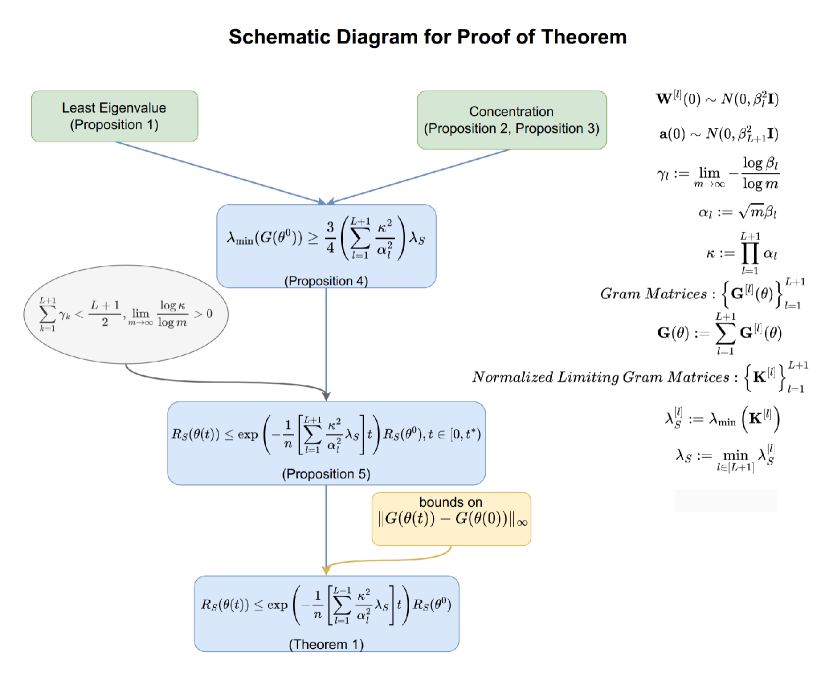
Figure 1: Sketch of proof for Theorem 1.

Theorem 1.

Suppose $\sigma(\cdot)$ satisfies conditions in Assumption 1, and $\mathcal{S}$ satisfies conditions in Assumption 2, if $\sum_{k=1}^{L+1}\gamma_{k}<\frac{L+1}{2}$, i.e., $\lim_{m\to\infty}\frac{\log\kappa}{\log m}>0$, and

$$m=\max\left\{\left(\Omega\left(\frac{n^{2}}{\lambda_{\mathcal{S}}^{2}}\log n\right)\right),\Omega\left(\left(\frac{n}{\lambda_{\mathcal{S}}}\right)^{\frac{1}{\frac{L+1}{2}-\sum_{k=1}^{L+1}\gamma_{k}}}\right),\Omega\left(\left(\frac{n}{\lambda_{\mathcal{S}}}\right)^{\frac{2}{\frac{L+1}{2}-\sum_{k=1}^{L+1}\gamma_{k}}}\right)\right\},$$

where $\lambda_{\mathcal{S}}=\min_{l\in[L+1]}\lambda_{\min}\left(\bm{K}^{[l]}\right)$, then with high probability, for any time $t\geq 0$,

$$R_{\mathcal{S}}(\bm{\theta}(t))\leq\exp\left(-\frac{1}{n}\left[\left(\sum_{l=1}^{L+1}\frac{\kappa^{2}}{\alpha_{l}^{2}}\right){\lambda_{\mathcal{S}}}\right]t\right)R_{\mathcal{S}}(\bm{\theta}(0)).$$ (4.37)

Moreover, for any time $t\geq 0$,

$$\left\{\begin{aligned} \lim_{m\to\infty}\frac{\left\lVert\bm{W}^{[l]}(t)-\bm{W}^{[l]}(0)\right\rVert_{\mathrm{F}}}{\left\lVert\bm{W}^{[l]}(0)\right\rVert_{\mathrm{F}}}=\frac{\left\lVert\frac{\overline{\bm{W}}^{[l]}(t)}{\sqrt{m}}-\frac{\overline{\bm{W}}^{[l]}(0)}{\sqrt{m}}\right\rVert_{\mathrm{F}}}{\left\lVert\frac{\overline{\bm{W}}^{[l]}(0)}{\sqrt{m}}\right\rVert_{\mathrm{F}}}&=0,~{}~{}l\in[L],\\ \lim_{m\to\infty}\frac{\left\lVert{{\bm{a}}(t)}-{{\bm{a}}(0)}\right\rVert_{2}}{\left\lVert{{\bm{a}}(0)}\right\rVert_{2}}=\lim_{m\to\infty}\frac{\left\lVert\frac{\bar{\bm{a}}(t)}{\sqrt{m}}-\frac{\bar{\bm{a}}(0)}{\sqrt{m}}\right\rVert_{2}}{\left\lVert\frac{\bar{\bm{a}}(0)}{\sqrt{m}}\right\rVert_{2}}&=0.\end{aligned}\right.$$ (4.38)

Remark 3.

The high probability specifically reads

• Event (I): Concentration between the normalized Gram matrices $\left\{\overline{\bm{G}}^{[l]}(\bm{\theta}^{0})\right\}_{l=1}^{L+1}$ and the normalized limiting Gram matrices $\left\{\bm{K}^{[l]}\right\}_{l=1}^{L+1}$;

  $$\mathbb{P}(I)\leq 2n^{2}L\exp\left(-\frac{2^{L}m\lambda_{\mathcal{S}}^{2}}{16n^{2}}\right).$$ (4.39)

• Event (II): Initial bounds on $\left\{\left\lVert\frac{\overline{\bm{W}}^{[l]}}{\sqrt{m}}\right\rVert_{2\to 2}\right\}_{l=1}^{L}$, $\left\{\left\lVert\frac{\overline{\bm{W}}^{[l]}}{\sqrt{m}}\right\rVert_{\mathrm{F}}\right\}_{l=1}^{L}$ and $\left\lVert\frac{\bar{\bm{a}}}{\sqrt{m}}\right\rVert_{2}$;

  $$\mathbb{P}(II)\leq 2(L-1)\exp\left(-\frac{m^{2}}{36}\right)+2\exp\left(-\frac{md}{36}\right)+2(L+1)\exp(-m).$$ (4.40)

Based on (4.39) and (4.40), by picking out the event I and II, lower bound of the high probability reads

$$1-\mathbb{P}(I)-\mathbb{P}(II) \geq 1-2n^{2}L\exp\left(-\frac{2^{L}m\lambda_{\mathcal{S}}^{2}}{16n^{2}}\right)$$

$$~{}~{}-\left[2(L-1)\exp\left(-\frac{m^{2}}{36}\right)+2\exp\left(-\frac{md}{36}\right)+2(L+1)\exp(-m)\right].$$

We remark that the establishment of relation (4.39) shall be traced back to Proposition 2 and Proposition 3, and the establishment of relation (4.40) is the combined effort of Lemma 5, Lemma 6, and Proposition 7.

5 Conclusions

In this paper, we propose a unified approach to characterize the theta-lazy regime for the $L$-layer NNs with a wide class of smooth activation functions. Our investigation reveals that the initial scale $\kappa$ of the output function is the pivotal factor for the propensity of the parameter set $\bm{\theta}$ to persist in its initialization state throughout the entire training process. This phenomenon holds true irrespective of the diverse array of initialization schemes employed, indicating the fundamental role played by the initial scale $\kappa$ in shaping the training dynamics of neural networks. In conclusion, our investigation into the statistical properties of the numerous parameters elucidates a macroscopic perspective on the study of neural networks.

One may inquire why the theta-lazy regime, as delineated in [20, 2], resides in the left-half plane of the line $\kappa=1$ rather than $\kappa=0$, as observed in this paper. It is imperative to note that our findings encompass the results in [20, 2]. However, in contrast to the normalization approach employed in [20, 2], wherein the parameters $\mathrm{vec}\left(\bm{a},\bm{W}\right)$ of the two-layer neural networks are normalized to $\mathrm{vec}\left(\bar{\bm{a}},\overline{\bm{W}}\right)$, we adopt a more general strategy designed for multi-layer NNs by normalizing the parameters to $\mathrm{vec}\left(\frac{\bar{\bm{a}}}{\sqrt{m}},\frac{\overline{\bm{W}}}{\sqrt{m}}\right)$. Consequently, in the scenario where $L=1$, corresponding to the case of two-layer NNs, it is reasonable for the threshold of $\kappa$ to shift by a distance of $\frac{1}{2}+\frac{1}{2}=1$. We anticipate that this formalism can be readily extended to the analysis of $L$-layer CNNs, where we hypothesize that the initial scale of the output function also serves as a critical factor for the persistence of weight parameters in their initialization state during training. However, we acknowledge the potential variability in this phenomenon for Residual Neural Networks (ResNet), which may hinge on the specific choice of initialization schemes, owing to their distinctive skip-connection architecture.

In our next paper, we aim to delineate the distinct characteristics exhibited by NNs in the area where $\lim_{m\to\infty}\frac{\log\kappa}{\log m}<0$, and we will provide a complete and detailed analysis for the transition across the boundary. Furthermore, we aspire to reveal the mechanism of initial condensation for multi-layer NNs, and to identify the directions towards which the weight parameters condense. The synthesis of these two papers holds promise in furnishing a nuanced understanding of the implicit regularization effects engendered by weight initialization schemes, thereby serving as a cornerstone upon which future works can be done to provide thorough characterization of the dynamical behavior of general NNs at each of the identified regime.

Appendix A Full Rankness of Gram Matrices

A.1 Some Technical Lemmas

Lemma 1.

Suppose $\sigma(\cdot)$ satisfies conditions in Assumption 1, consider input data $\mathcal{Z}:=\{\bm{z}_{1},\bm{z}_{2},\dots,\bm{z}_{n}\}$ comprising $n$ non-parallel unit samples, given any $\varepsilon>0$, we define

$$\bm{G}_{\varepsilon}(\mathcal{Z}):=\left[\bm{G}_{\varepsilon}(\mathcal{Z})_{ij}\right]:=\left[\mathbb{E}_{\bm{w}\sim\mathcal{N}\left(\bm{0},\bm{I}_{d}\right)}\frac{\sigma(\varepsilon\bm{w}^{\intercal}\bm{z}_{i})}{\varepsilon}\frac{\sigma(\varepsilon\bm{w}^{\intercal}\bm{z}_{j})}{\varepsilon}\right],$$ (A.1)

then there exists constant $\lambda_{\mathcal{Z}}>0$ independent of $\varepsilon$, such that

$$\lambda_{\min}\left(\bm{G}_{\varepsilon}(\mathcal{Z})\right)\geq\lambda_{\mathcal{Z}}.$$ (A.2)

Proof.

We observe that as $\varepsilon\to 0$, the limiting entries of $\bm{G}_{\varepsilon}(\mathcal{Z})$, denoted by $\bm{G}_{0}(\mathcal{Z})$ read

$$\bm{G}_{0}(\mathcal{Z})_{ij} :=\lim_{\varepsilon\to 0}\mathbb{E}_{\bm{w}\sim\mathcal{N}\left(\bm{0},\bm{I}_{d}\right)}\frac{\sigma(\varepsilon\bm{w}^{\intercal}\bm{z}_{i})\sigma(\varepsilon\bm{w}^{\intercal}\bm{z}_{j})}{\varepsilon^{2}}$$

$$=\mathbb{E}_{\bm{w}\sim\mathcal{N}\left(\bm{0},\bm{I}_{d}\right)}\left[(\bm{w}^{\intercal}\bm{z}_{i})(\bm{w}^{\intercal}\bm{z}_{j})\right]=\left<\bm{z}_{i},\bm{z}_{j}\right>,$$

and since $\bm{z}_{i}$ and $\bm{z}_{j}$ are non-parallel with each other, then $\lambda_{0}:=\lambda_{\min}\left(\bm{G}_{0}(\mathcal{Z})\right)>0$, and it depends solely on the data.

In the case where $\varepsilon\to\infty$, as the limit reads

$$\lim_{\varepsilon\to 0}\frac{\sigma(\varepsilon\bm{w}^{\intercal}\bm{z}_{i})\sigma(\varepsilon\bm{w}^{\intercal}\bm{z}_{j})}{\varepsilon^{2}}=(\bm{w}^{\intercal}\bm{z}_{i})(\bm{w}^{\intercal}\bm{z}_{j})\left(a\mathbf{1}_{\bm{w}^{\intercal}\bm{z}_{i}<0}+b\mathbf{1}_{\bm{w}^{\intercal}\bm{z}_{i}>0}\right)\left(a\mathbf{1}_{\bm{w}^{\intercal}\bm{z}_{j}<0}+b\mathbf{1}_{\bm{w}^{\intercal}\bm{z}_{j}>0}\right),$$

then as $\varepsilon\to\infty$, the limiting entries of $\bm{G}_{\varepsilon}(\mathcal{Z})$, denoted by $\bm{G}_{\infty}(\mathcal{Z})$, shares the character of the ReLU NTK. Specifically, if we choose $a=0$ and $b=\sqrt{2}$, then

$$\bm{G}_{\infty}(\mathcal{Z})_{ij} :=\lim_{\varepsilon\to\infty}\mathbb{E}_{\bm{w}\sim\mathcal{N}\left(\bm{0},\bm{I}_{d}\right)}\frac{\sigma(\varepsilon\bm{w}^{\intercal}\bm{z}_{i})\sigma(\varepsilon\bm{w}^{\intercal}\bm{z}_{j})}{\varepsilon^{2}}$$

$$=\frac{1}{\pi}\left(\left<\bm{z}_{i},\bm{z}_{j}\right>(\pi-\arccos{\left<\bm{z}_{i},\bm{z}_{j}\right>})+\sqrt{1-\left<\bm{z}_{i},\bm{z}_{j}\right>^{2}}\right),$$

and since $\bm{z}_{i}$ and $\bm{z}_{j}$ are non-parallel with each other, then $\lambda_{\infty}:=\lambda_{\min}\left(\bm{G}_{\infty}(\mathcal{Z})\right)>0$, and it depends solely on the data and activation function.

Moreover, as $\lambda_{\min}\left(\bm{G}_{\varepsilon}(\mathcal{Z})\right)$ is a continuous function with respect to the entries of $\bm{G}_{\varepsilon}(\mathcal{Z})$, we conclude that there exists $\varepsilon_{1}<1$, such that for any $\varepsilon\in(0,\varepsilon_{1}]$, $\lambda_{\min}\left(\bm{G}_{\varepsilon}(\mathcal{Z})\right)\geq\frac{1}{2}\lambda_{0}.$ Similarly, there also exists $M_{1}>1$, such that for any $\varepsilon\in[M_{1},\infty)$, $\lambda_{\min}\left(\bm{G}_{\varepsilon}(\mathcal{Z})\right)\geq\frac{1}{2}\lambda_{\infty}.$ Finally, Lemma $\mathrm{F.1.}$ in Du et al. [7] guarantees that: For any $\varepsilon\in[\varepsilon_{1},M_{1}]$, $\lambda_{\min}\left(\bm{G}_{\varepsilon}(\mathcal{Z})\right)>0,$ and by choosing

$$\lambda_{\mathcal{Z}}:=\min\left\{\frac{1}{2}\lambda_{0},\frac{1}{2}\lambda_{\infty},\min_{\varepsilon\in[\varepsilon_{1},M_{1}]}\lambda_{\min}\left(\bm{G}_{\varepsilon}(\mathcal{Z})\right)\right\},$$

we finish our proof. ∎

Lemma 2.

If $\bm{A}:=[a_{ij}]_{n\times n}$ is semi-positive definite, and $\bm{B}:=[b_{ij}]_{n\times n}$ is positive definite, then

$$\lambda_{\min}(\bm{A}\odot\bm{B})\geq\left(\frac{n-1}{n}\right)^{\frac{n-1}{2}}\left(\prod_{i=1}^{n}{a_{ii}}\right)\mathrm{det}(\bm{B}).$$ (A.3)

Proof.

By application of Oppenheim inequality [16, Theorem 7.8.16], the following holds

$$\mathrm{det}(\bm{A}\odot\bm{B})\geq\left(\prod_{i=1}^{n}{a_{ii}}\right)\mathrm{det}(\bm{B}).$$

Moreover, Hong and Pan [15] provided a lower bound for the least eigenvalue, wherein for a semi-positive definite matrix $\bm{C}=[c_{ij}]_{n\times n}$, its least eigenvalue yields the following estimate

$$\lambda_{\min}(\bm{C})\geq\left(\frac{n-1}{n}\right)^{\frac{n-1}{2}}\mathrm{det}(\bm{C}),$$

thus we obtain that

$$\lambda_{\min}(\bm{A}\odot\bm{B})\geq\left(\frac{n-1}{n}\right)^{\frac{n-1}{2}}\left(\prod_{i=1}^{n}{a_{ii}}\right)\mathrm{det}(\bm{B}).$$

∎

Lemma 3.

Suppose $\sigma(\cdot)$ satisfies conditions in Assumption 1, and we assume that there exists some constant $c>0$ and $\gamma>0$, such that

$$\bm{A}_{1}:=\left[\begin{array}[]{cc}a_{1}^{2}&\rho_{1}a_{1}b_{1}\\ \rho_{1}a_{1}b_{1}&b_{1}^{2}\end{array}\right],~{}~{}\bm{A}_{2}:=\left[\begin{array}[]{cc}a_{2}^{2}&\rho_{2}a_{2}b_{2}\\ \rho_{2}a_{2}b_{2}&b_{2}^{2}\end{array}\right],$$

where for any $l\in[2]$,

$$\frac{1}{c}\leq\min\{a_{l},b_{l}\},~{}~{}\max\{a_{l},b_{l}\}\leq c,$$ (A.4)

and

$$-1+\gamma\leq\rho_{l}\leq 1-\gamma,$$ (A.5)

then for some fixed $\varepsilon>0$, as we define

$$F(\bm{A}) :=\mathbb{E}_{(u,v)\sim\mathcal{N}(\mathbf{0},\bm{A})}\left[\frac{\sigma(\varepsilon u)}{\varepsilon}\frac{\sigma(\varepsilon v)}{\varepsilon}\right],$$

$$G(\bm{A}) :=\mathbb{E}_{(u,v)\sim\mathcal{N}(\mathbf{0},\bm{A})}\left[{\sigma^{(1)}(\varepsilon u)}{\sigma^{(1)}(\varepsilon v)}\right],$$

the following holds

$$\max\left\{\left\lvert F(\bm{A}_{1})-F(\bm{A}_{2})\right\rvert,\left\lvert G(\bm{A}_{1})-G(\bm{A}_{2})\right\rvert\right\}\leq C\left\lVert\bm{A}_{1}-\bm{A}_{2}\right\rVert_{\infty},$$ (A.6)

for some constant $C>0$ that depends sorely on $c$, $\gamma$, and $\sigma(\cdot)$, and independent of $\varepsilon$.

Proof.

Let

$$\bm{A}=\left[\begin{array}[]{cc}a^{2}&\rho ab\\ \rho ab&b^{2}\end{array}\right]$$

with

$$\min\{a_{1},a_{2}\}\leq a\leq\max\{a_{1},a_{2}\},~{}~{}\min\{b_{1},b_{2}\}\leq b\leq\max\{b_{1},b_{2}\}$$

and

$$-1+\gamma\leq\rho\leq 1-\gamma,$$

then

$$F(\bm{A}) =\mathbb{E}_{(z_{1},z_{2})\sim\mathcal{N}(\mathbf{0},\bm{B})}\left[\frac{\sigma(\varepsilon az_{1})}{\varepsilon}\frac{\sigma(\varepsilon bz_{2})}{\varepsilon}\right],$$

$$G(\bm{A}) =\mathbb{E}_{(z_{1},z_{2})\sim\mathcal{N}(\mathbf{0},\bm{B})}\left[{\sigma^{(1)}(\varepsilon az_{1})}{\sigma^{(1)}(\varepsilon bz_{2})}\right],$$

with

$$\bm{B}:=\left[\begin{array}[]{cc}1&\rho\\ \rho&1\end{array}\right].$$

Then, we obtain that

$$\left\lvert\frac{\partial F(\bm{A})}{\partial a}\right\rvert =\left\lvert\mathbb{E}_{(z_{1},z_{2})\sim\mathcal{N}(\mathbf{0},\bm{B})}\left[\sigma^{(1)}(\varepsilon az_{1})z_{1}\frac{\sigma(\varepsilon bz_{2})}{\varepsilon}\right]\right\rvert$$

$$\leq\left[\mathbb{E}_{z_{1}\sim\mathcal{N}(0,1)}\left(\sigma^{(1)}(\varepsilon az_{1})\right)^{2}z_{1}^{2}\right]^{1/2}\left[\mathbb{E}_{z_{2}\sim\mathcal{N}(0,1)}\left(\frac{\sigma(\varepsilon bz_{2})}{\varepsilon}\right)^{2}\right]^{1/2}$$

$$\leq C(\mathbb{E}_{z_{1}\sim\mathcal{N}(0,1)}z_{1}^{2})^{1/2}\left[\mathbb{E}_{z_{2}\sim\mathcal{N}(0,1)}\left(\sigma^{(1)}(\varepsilon\theta bz_{2})\right)^{2}b^{2}z_{2}^{2}\right]^{1/2}\leq C^{2}b\leq C^{2}c,$$

and by similar reasoning, $\left\lvert\frac{\partial F(\bm{A})}{\partial b}\right\rvert\leq C^{2}c$. As for the estimate of $\left\lvert\frac{\partial F(\bm{A})}{\partial\rho}\right\rvert$, we observe that

$$\left\lvert F(\bm{A})\right\rvert =\left\lvert\mathbb{E}_{(z_{1},z_{2})\sim\mathcal{N}(\mathbf{0},\bm{B})}\left[\frac{\sigma(\varepsilon az_{1})}{\varepsilon}\frac{\sigma(\varepsilon bz_{2})}{\varepsilon}\right]\right\rvert$$ (A.7)

$$\leq\left[\mathbb{E}_{z_{1}\sim\mathcal{N}(0,1)}\left(\frac{\sigma(\varepsilon az_{1})}{\varepsilon}\right)^{2}\right]^{1/2}\left[\mathbb{E}_{z_{2}\sim\mathcal{N}(0,1)}\left(\frac{\sigma(\varepsilon az_{2})}{\varepsilon}\right)^{2}\right]^{1/2}\leq C^{2}c^{2},$$

and for any $\varepsilon>0$, $\frac{\sigma(\varepsilon az)}{\varepsilon}$ and $\frac{\sigma(\varepsilon bz)}{\varepsilon}$ belong to the Gaussian function space

$$\mathcal{L}^{2}\left(\mathbb{R},\exp\left(-\frac{z^{2}}{2}\right)\right):=\left\{f~{}\middle|~{}\int_{\mathbb{R}}f(z)\exp\left(-\frac{z^{2}}{2}\right)\mathrm{d}z<\infty\right\},$$ (A.8)

with the Hermite expansion of $\frac{\sigma(\varepsilon az_{1})}{\varepsilon}$ reads

$$\frac{\sigma(\varepsilon az_{1})}{\varepsilon}:=\sum_{k=0}^{\infty}\alpha_{k}H_{k}(z_{1}),$$

while the Hermite expansion of $\frac{\sigma(\varepsilon bz_{2})}{\varepsilon}$ reads

$$\frac{\sigma(\varepsilon bz_{2})}{\varepsilon}:=\sum_{k=0}^{\infty}\beta_{k}H_{k}(z_{2}),$$

where $\{H_{k}(\cdot)\}_{k=0}^{\infty}$ are the probabilist’s Hermite polynomials, and $\{\alpha_{k}\}_{k=0}^{\infty}$ and $\{\beta_{k}\}_{k=0}^{\infty}$ depend on the choice of $\varepsilon$. Then, we obtain that

$$F(\bm{A}) =\mathbb{E}_{(z_{1},z_{2})\sim\mathcal{N}(\mathbf{0},\bm{B})}\left[\frac{\sigma(\varepsilon az_{1})}{\varepsilon}\frac{\sigma(\varepsilon bz_{2})}{\varepsilon}\right]$$

$$=\mathbb{E}\left[\left(\sum_{k=0}^{\infty}\alpha_{k}H_{k}(z_{1})\right)\left(\sum_{l=0}^{\infty}\beta_{l}H_{l}(z_{2})\right)\right]$$

$$=\mathbb{E}\left[\sum_{k,l=0}^{\infty}\alpha_{k}\beta_{l}H_{k}(z_{1})H_{l}(z_{2})\right]=\sum_{k,l=0}^{\infty}\alpha_{k}\beta_{l}k!\left(\mathbb{E}\left[z_{1}z_{2}\right]\right)^{k}\delta_{k}^{l}=\sum_{k=0}^{\infty}\alpha_{k}\beta_{k}k!\rho^{k}.$$

As is shown by relation (A.7), the power series $F(\bm{A})=\sum_{k=0}^{\infty}\alpha_{k}\beta_{k}k!\rho^{k}$ is absolute convergent for any $\rho\in(-1,1)$, hence by differentiation, the power series

$$\sum_{k=0}^{\infty}\alpha_{k+1}\beta_{k+1}(k+1)!(k+1)\rho^{k}$$

is absolute convergent for any $\rho\in(-1,1)$, and it converges uniformly to $\frac{\partial F(\bm{A})}{\partial\rho}$, thus we obtain that for any $\rho\in[-1+\gamma,1-\gamma]$, $\left\lvert\frac{\partial F(\bm{A})}{\partial\rho}\right\rvert\leq C.$

As for $\bm{G}(\bm{A})$, we remark that for any $\varepsilon>0$,

$$\left\lvert G(\bm{A})\right\rvert=\left\lvert\mathbb{E}_{(z_{1},z_{2})\sim\mathcal{N}(\mathbf{0},\bm{B})}\left[{\sigma^{(1)}(\varepsilon az_{1})}{\sigma^{(1)}(\varepsilon bz_{2})}\right]\right\rvert\leq C^{2},$$ (A.9)

as we send $\varepsilon\to 0$,

$$\lim_{\varepsilon\to 0}G(\bm{A})=\lim_{\varepsilon\to 0}\mathbb{E}_{(z_{1},z_{2})\sim\mathcal{N}(\mathbf{0},\bm{B})}\left[{\sigma^{(1)}(\varepsilon az_{1})}{\sigma^{(1)}(\varepsilon bz_{2})}\right]=\mathbb{E}_{(z_{1},z_{2})\sim\mathcal{N}(\mathbf{0},\bm{B})}\left[{\sigma^{(1)}(0)}\right]^{2}=1,$$

and as we send $\varepsilon\to\infty$,

$$\lim_{\varepsilon\to\infty}G(\bm{A}) =\lim_{\varepsilon\to\infty}\mathbb{E}_{(z_{1},z_{2})\sim\mathcal{N}(\mathbf{0},\bm{B})}\left[{\sigma^{(1)}(\varepsilon az_{1})}{\sigma^{(1)}(\varepsilon bz_{2})}\right]$$

$$=\mathbb{E}_{(z_{1},z_{2})\sim\mathcal{N}(\mathbf{0},\bm{B})}\left[\left(a\mathbf{1}_{z_{1}<0}+b\mathbf{1}_{z_{1}>0}\right)\left(a\mathbf{1}_{z_{2}<0}+b\mathbf{1}_{z_{2}>0}\right)\right]$$

$$=a^{2}\mathbb{E}_{(z_{1},z_{2})\sim\mathcal{N}(\mathbf{0},\bm{B})}\mathbf{1}_{z_{1}<0,z_{2}<0}+ab\mathbb{E}_{(z_{1},z_{2})\sim\mathcal{N}(\mathbf{0},\bm{B})}\mathbf{1}_{z_{1}<0,z_{2}>0}$$

$$~{}~{}+ab\mathbb{E}_{(z_{1},z_{2})\sim\mathcal{N}(\mathbf{0},\bm{B})}\mathbf{1}_{z_{1}>0,z_{2}<0}+b^{2}\mathbb{E}_{(z_{1},z_{2})\sim\mathcal{N}(\mathbf{0},\bm{B})}\mathbf{1}_{z_{1}>0,z_{2}>0}$$

$$=\frac{a^{2}+b^{2}}{2\pi}\left(\pi-\arccos{\rho}\right)+\frac{ab}{\pi}\arccos{\rho},$$

hence by dominated convergence theorem, as $-1+\gamma\leq\rho\leq 1-\gamma,$ we obtain that

$$\lim_{\varepsilon\to 0}\left\lvert G(\bm{A}_{1})-G(\bm{A}_{2})\right\rvert =0,$$

$$\lim_{\varepsilon\to\infty}\left\lvert G(\bm{A}_{1})-G(\bm{A}_{2})\right\rvert \leq C\left\lvert\rho_{1}-\rho_{2}\right\rvert\leq C\left\lVert\bm{A}_{1}-\bm{A}_{2}\right\rVert_{\infty}.$$

Since $G(\bm{A})$ is continuous in $\varepsilon$, then there exists $\varepsilon_{1}<1$, such that for any $\varepsilon\in(0,\varepsilon_{1}]$,

$$\left\lvert G(\bm{A}_{1})-G(\bm{A}_{2})\right\rvert\leq\left\lVert\bm{A}_{1}-\bm{A}_{2}\right\rVert_{\infty},$$ (A.10)

by similar reasoning, there also exists $M_{1}>1$, such that for any $\varepsilon\in[M_{1},\infty)$,

$$\left\lvert G(\bm{A}_{1})-G(\bm{A}_{2})\right\rvert\leq 2C\left\lVert\bm{A}_{1}-\bm{A}_{2}\right\rVert_{\infty}.$$ (A.11)

Finally, for any $\varepsilon\in[\varepsilon_{1},M_{1}]$,

$$\left\lvert\frac{\partial G(\bm{A})}{\partial a}\right\rvert =\left\lvert\mathbb{E}_{(z_{1},z_{2})\sim\mathcal{N}(\mathbf{0},\bm{B})}\left[{\sigma^{(2)}(\varepsilon az_{1})}\varepsilon z_{1}{\sigma^{(1)}(\varepsilon bz_{2})}\right]\right\rvert$$

$$\leq C\left\lvert\mathbb{E}_{z_{1}\sim\mathcal{N}(0,1)}\varepsilon z_{1}\right\rvert\leq 2CM_{1},$$

and

$$\left\lvert\frac{\partial G(\bm{A})}{\partial b}\right\rvert =\left\lvert\mathbb{E}_{(z_{1},z_{2})\sim\mathcal{N}(\mathbf{0},\bm{B})}\left[{\sigma^{(1)}(\varepsilon az_{1})}{\sigma^{(1)}(\varepsilon bz_{2})\varepsilon z_{1}}\right]\right\rvert$$

$$\leq C\left\lvert\mathbb{E}_{z_{2}\sim\mathcal{N}(0,1)}\varepsilon z_{2}\right\rvert\leq 2CM_{1}.$$

Moreover, for any $\varepsilon>0$, ${\sigma^{(1)}(\varepsilon az_{1})}$ and ${\sigma^{(1)}(\varepsilon bz_{2})}$ belong to the Gaussian function space demonstrated in (A.8), then by similar reasoning, as we expand $G(\bm{A})$ in the power series of $\rho$, since the power is absolute convergent for any $\rho\in(-1,1)$, then its differentiation is also absolute convergent for any $\rho\in(-1,1)$, and it converges uniformly to $\frac{\partial G(\bm{A})}{\partial\rho}$. Thus, we obtain that for any $\rho\in[-1+\gamma,1-\gamma]$, $\left\lvert\frac{\partial G(\bm{A})}{\partial\rho}\right\rvert\leq C.$

We remark that as relation (A.10) and (A.11) partially finish the proof of relation (A.6), therefore, we focus on $F(\bm{A})$ for any $\varepsilon>0$, and $G(\bm{A})$ for any $\varepsilon\in[\varepsilon_{1},M_{1}]$. There exists $C>0$ independent of $a$, $b$ and $\rho$, such that

$$\left\lvert\frac{\partial F(\bm{A})}{\partial a}\right\rvert \leq C,~{}~{}\left\lvert\frac{\partial F(\bm{A})}{\partial b}\right\rvert\leq C,~{}~{}\left\lvert\frac{\partial F(\bm{A})}{\partial\rho}\right\rvert\leq C,$$

$$\left\lvert\frac{\partial G(\bm{A})}{\partial a}\right\rvert \leq C,~{}~{}\left\lvert\frac{\partial G(\bm{A})}{\partial b}\right\rvert\leq C,~{}~{}\left\lvert\frac{\partial G(\bm{A})}{\partial\rho}\right\rvert\leq C,$$

and we proceed to bound $\nabla_{\bm{A}}F(\bm{A})$ and $\nabla_{\bm{A}}G(\bm{A})$. Since for the set

$$\mathcal{M}:=\left\{(a,b,\rho):\frac{1}{c}\leq a\leq c,~{}~{}\frac{1}{c}\leq b\leq c,~{}~{}-1+\gamma\leq\rho\leq 1-\gamma\right\},$$

there exists a $\mathcal{C}^{\infty}$-mapping $\bm{\phi}(\cdot):\mathcal{M}\to\mathbb{R}^{3}$, where

$$\bm{\phi}(a,b,\rho)=[a^{2},b^{2},\rho ab]^{\intercal},$$

as the Jacobian of $\bm{\phi}$ at any point $\bm{z}:=(a,b,\rho)\in\mathcal{M}$ reads

$$J_{\bm{\phi}}(\bm{z})=\mathrm{det}\left[\frac{\partial\bm{\phi}(\bm{z})}{\partial(a,b,\rho)}\right]=\mathrm{det}\left[\begin{array}[]{ccc}2a&0&0\\ 0&2b&0\\ \rho b&\rho a&ab\end{array}\right]=4a^{2}b^{2}>0,$$

indicating that $\bm{\phi}(\cdot)$ is a $1$-$1$ mapping on the domain $\mathcal{M}$. Moreover, since we have

$$\nabla_{\bm{A}}F(\bm{A})=\left[\frac{\partial\bm{\phi}(\bm{z})}{\partial(a,b,\rho)}\right]^{-1}\nabla_{\bm{z}}F(\bm{A}),~{}~{}\nabla_{\bm{A}}G(\bm{A})=\left[\frac{\partial\bm{\phi}(\bm{z})}{\partial(a,b,\rho)}\right]^{-1}\nabla_{\bm{z}}G(\bm{A}),$$

and as $\max\left\{\left\lVert\nabla_{\bm{z}}F(\bm{A})\right\rVert_{\infty},\left\lVert\nabla_{\bm{z}}G(\bm{A})\right\rVert_{\infty}\right\}\leq C$, then the following holds

$$\max\left\{\left\lVert\nabla_{\bm{A}}F(\bm{A})\right\rVert_{2},\left\lVert\nabla_{\bm{A}}G(\bm{A})\right\rVert_{2}\right\} \leq\left\lVert\left[\frac{\partial\bm{\phi}(\bm{z})}{\partial(a,b,\rho)}\right]^{-1}\right\rVert_{2\to 2}\max\left\{\left\lVert\nabla_{\bm{z}}F(\bm{A})\right\rVert_{2},\left\lVert\nabla_{\bm{z}}G(\bm{A})\right\rVert_{2}\right\}$$

$$\leq\max\left\{\frac{1}{2a},~{}~{}\frac{1}{2b},~{}~{}\frac{1}{ab}\right\}\sqrt{3}C\leq cC,$$

and as all norms are equivalent in finite dimensional vector spaces, we finish the proof. ∎

Our next lemma aims to demonstrate validity of relation (A.4) imposed in Lemma 3.

Lemma 4.

Suppose $\sigma(\cdot)$ satisfies conditions in Assumption 1, and given

$$\frac{1}{c}\leq x_{0}\leq c,$$ (A.12)

for some constant $c>0$, then for any $\varepsilon>0$, there exist some constants $\mu_{1},\mu_{2}>0$ satisfying

$$\left\{\begin{aligned} \mu_{1}x_{0}^{2}&\leq\mathbb{E}_{u\sim\mathcal{N}(0,x_{0}^{2})}\left[\frac{\sigma(\varepsilon u)}{\varepsilon}\right]^{2}\leq\mu_{2}x_{0}^{2},\\ \mu_{1}&\leq\mathbb{E}_{u\sim\mathcal{N}(0,x_{0}^{2})}\left[\sigma^{(1)}(\varepsilon u)\right]^{2}\leq\mu_{2},\end{aligned}\right.$$ (A.13)

where $\mu_{1}$ and $\mu_{2}$ are independent of $\varepsilon$.

Proof.

Directly from Assumption 1, we obtain that

$$\frac{\sigma(\varepsilon u)}{\varepsilon}\leq Cu,~{}~{}\sigma^{(1)}(\varepsilon u)\leq C,$$

where $C$ is the Lipschitz constant in Assumption 1, by taking expectations

$$\mathbb{E}_{u\sim\mathcal{N}(0,x_{0}^{2})}\left[\frac{\sigma(\varepsilon u)}{\varepsilon}\right]^{2} \leq C^{2}\mathbb{E}_{u\sim\mathcal{N}(0,x_{0}^{2})}u^{2}=C^{2}x_{0}^{2},$$

$$\mathbb{E}_{u\sim\mathcal{N}(0,x_{0}^{2})}\left[\sigma^{(1)}(\varepsilon u)\right]^{2} \leq C^{2},$$

as we set $\mu_{2}:=C$, we partially finish the proof for relation (A.13).

As for $\mu_{1}$, we define auxiliary functions $F(\cdot;x_{0}):[0,+\infty)\to\mathbb{R}$,

$$F(\varepsilon;x_{0}):=\left\{\begin{array}[]{ll}\mathbb{E}_{u\sim\mathcal{N}(0,x_{0}^{2})}\left[\frac{\sigma(\varepsilon u)}{\varepsilon}\right]^{2},&\varepsilon\neq 0,\\ \mathbb{E}_{u\sim\mathcal{N}(0,x_{0}^{2})}u^{2},&\varepsilon=0,\end{array}\right.$$ (A.14)

where $x_{0}>0$ is a fixed constant. For function $F(\cdot;x_{0})$, as $\varepsilon\to 0^{+}$,

$$\lim_{\varepsilon\to 0^{+}}\frac{\sigma(\varepsilon u)}{\varepsilon}=\lim_{\varepsilon\to 0^{+}}\frac{\left[\sigma(0)+\sigma^{(1)}(0)\varepsilon u+o(\varepsilon)\right]}{\varepsilon}=u,$$

by taking expectation on both sides, we obtain that

$$\lim_{\varepsilon\to 0^{+}}\mathbb{E}_{u\sim\mathcal{N}(0,x_{0}^{2})}\left[\frac{\sigma(\varepsilon u)}{\varepsilon}\right]^{2}=\mathbb{E}_{u\sim\mathcal{N}(0,x_{0}^{2})}u^{2}=x_{0}^{2}.$$ (A.15)

$F(\cdot;x_{0})$ is continuous on $[0,+\infty)$, and there exists $\varepsilon_{1}<1$, such that for any $\varepsilon\in(0,\varepsilon_{1}]$,

$$\mathbb{E}_{u\sim\mathcal{N}(0,x_{0}^{2})}\left[\frac{\sigma(\varepsilon u)}{\varepsilon}\right]^{2}\geq\frac{1}{2}x_{0}^{2}.$$ (A.16)

Moreover, as $\varepsilon\to\infty$,

$$\lim_{\varepsilon\to+\infty}\frac{\sigma(\varepsilon u)}{\varepsilon}=\left\{\begin{array}[]{ll}a,&u<0,\\ 0,&u=0,\\ b,&u>0,\end{array}\right.$$

then by taking expectation on both sides, we obtain that

$$\lim_{\varepsilon\to+\infty}\mathbb{E}_{u\sim\mathcal{N}(0,x_{0}^{2})}\left[\frac{\sigma(\varepsilon u)}{\varepsilon}\right]^{2} =\mathbb{E}_{u\sim\mathcal{N}(0,x_{0}^{2})}\left[a^{2}u^{2}\mathbf{1}_{u<0}\right]+\mathbb{E}_{u\sim\mathcal{N}(0,x_{0}^{2})}\left[b^{2}u^{2}\mathbf{1}_{u>0}\right]$$ (A.17)

$$=\frac{a^{2}x_{0}^{2}}{2}+\frac{b^{2}x_{0}^{2}}{2}=\left(\frac{a^{2}+b^{2}}{2}\right)x_{0}^{2}.$$

By similar reasoning, there also exists $M_{1}>1$, such that for any $\varepsilon\in[M_{1},\infty)$,

$$\mathbb{E}_{u\sim\mathcal{N}(0,x_{0}^{2})}\left[\frac{\sigma(\varepsilon u)}{\varepsilon}\right]^{2}\geq\left(\frac{a^{2}+b^{2}}{4}\right)x_{0}^{2}.$$ (A.18)

Finally, as $\sigma^{(1)}(0)=1$ and $\sigma^{(1)}(\cdot)$ is continuous on $\mathbb{R}$, there exists $\widetilde{M}>0$, such that for any $s\in[-\widetilde{M},\widetilde{M}]$, $\sigma^{(1)}(s)\geq\frac{1}{2}.$ Then, for any $u\in\left[-\frac{\widetilde{M}}{M_{1}},\frac{\widetilde{M}}{M_{1}}\right]$ and $\varepsilon\in[\varepsilon_{1},M_{1}]$,

$$\mathbb{E}_{u\sim\mathcal{N}(0,x_{0}^{2})}\left[\frac{\sigma(\varepsilon u)}{\varepsilon}\right]^{2} \geq\mathbb{E}_{u\sim\mathcal{N}(0,x_{0}^{2})}\left[\frac{\sigma(\varepsilon u)}{\varepsilon}\mathbf{1}_{-\frac{\widetilde{M}}{M_{1}}\leq u\leq\frac{\widetilde{M}}{M_{1}}}\right]^{2}$$ (A.19)

$$\geq\frac{1}{4}\mathbb{E}_{u\sim\mathcal{N}(0,x_{0}^{2})}u^{2}\mathbf{1}_{-\frac{\widetilde{M}}{M_{1}}\leq u\leq\frac{\widetilde{M}}{M_{1}}}$$

$$\geq\left(\frac{1}{4}\mathbb{E}_{z\sim\mathcal{N}(0,1)}z^{2}\mathbf{1}_{-\frac{\widetilde{M}}{cM_{1}}\leq z\leq\frac{\widetilde{M}}{cM_{1}}}\right)x_{0}^{2}.$$

We define another auxiliary function $G(\cdot;x_{0}):[0,+\infty)\to\mathbb{R}$,

$$G(\varepsilon;x_{0}):=\left\{\begin{array}[]{ll}\mathbb{E}_{u\sim\mathcal{N}(0,x_{0}^{2})}\left[\sigma^{(1)}(\varepsilon u)\right]^{2},&\varepsilon\neq 0,\\ 1,&\varepsilon=0,\end{array}\right.$$ (A.20)

where $x_{0}>0$ is a fixed constant. For function $G(\cdot;x_{0})$, as $\varepsilon\to 0^{+}$,

$$\lim_{\varepsilon\to 0^{+}}\sigma^{(1)}(\varepsilon u)=\lim_{\varepsilon\to 0^{+}}\sigma^{(1)}(0)=1,$$

by taking expectation on both sides, we obtain that

$$\lim_{\varepsilon\to 0^{+}}\mathbb{E}_{u\sim\mathcal{N}(0,x_{0}^{2})}\left[\sigma^{(1)}(\varepsilon u)\right]^{2}=\mathbb{E}_{u\sim\mathcal{N}(0,x_{0}^{2})}1=1.$$ (A.21)

$G(\cdot;x_{0})$ is continuous on $[0,+\infty)$, and there exists $\varepsilon_{1}<1$, such that for any $\varepsilon\in(0,\varepsilon_{1}]$,

$$\mathbb{E}_{u\sim\mathcal{N}(0,x_{0}^{2})}\left[\sigma^{(1)}(\varepsilon u)\right]^{2}\geq\frac{1}{2}.$$ (A.22)

Moreover, as $\varepsilon\to\infty$,

$$\lim_{\varepsilon\to+\infty}\sigma^{(1)}(\varepsilon u)=\left\{\begin{array}[]{ll}a,&u<0,\\ 1,&u=0,\\ b,&u>0,\end{array}\right.$$

then by taking expectation on both sides, we obtain that

$$\lim_{\varepsilon\to+\infty}\mathbb{E}_{u\sim\mathcal{N}(0,x_{0}^{2})}\left[\sigma^{(1)}(\varepsilon u)\right]^{2} =\mathbb{E}_{u\sim\mathcal{N}(0,x_{0}^{2})}\left[a^{2}\mathbf{1}_{u<0}\right]+\mathbb{E}_{u\sim\mathcal{N}(0,x_{0}^{2})}\left[b^{2}\mathbf{1}_{u>0}\right]$$ (A.23)

$$=\frac{a^{2}+b^{2}}{2}.$$

Then, by similar reasoning, there also exists $M_{1}>1$, such that for any $\varepsilon\in[M_{1},\infty)$,

$$\mathbb{E}_{u\sim\mathcal{N}(0,x_{0}^{2})}\left[\sigma^{(1)}(\varepsilon u)\right]^{2}\geq\frac{a^{2}+b^{2}}{4}.$$ (A.24)

Finally, as $\sigma^{(1)}(0)=1$ and $\sigma^{(1)}(\cdot)$ is continuous on $\mathbb{R}$, there exists $\widetilde{M}>0$, such that for any $s\in[-\widetilde{M},\widetilde{M}]$, $\sigma^{(1)}(s)\geq\frac{1}{2}.$ Then, for any $u\in\left[-\frac{\widetilde{M}}{M_{1}},\frac{\widetilde{M}}{M_{1}}\right]$ and $\varepsilon\in[\varepsilon_{1},M_{1}]$,

$$\mathbb{E}_{u\sim\mathcal{N}(0,x_{0}^{2})}\left[\sigma^{(1)}(\varepsilon u)\right]^{2} \geq\mathbb{E}_{u\sim\mathcal{N}(0,x_{0}^{2})}\left[\sigma^{(1)}(\varepsilon u)\mathbf{1}_{-\frac{\widetilde{M}}{M_{1}}\leq u\leq\frac{\widetilde{M}}{M_{1}}}\right]^{2}$$ (A.25)

$$\geq\frac{1}{4}\mathbb{E}_{u\sim\mathcal{N}(0,x_{0}^{2})}\mathbf{1}_{-\frac{\widetilde{M}}{M_{1}}\leq u\leq\frac{\widetilde{M}}{M_{1}}}$$

$$\geq\left(\frac{1}{4}\mathbb{E}_{z\sim\mathcal{N}(0,1)}\mathbf{1}_{-\frac{\widetilde{M}}{cM_{1}}\leq z\leq\frac{\widetilde{M}}{cM_{1}}}\right),$$

Therefore, we set

$$\mu_{1}:=\min\left\{\frac{1}{2},\frac{a^{2}+b^{2}}{4},\left(\frac{1}{4}\mathbb{E}_{z\sim\mathcal{N}(0,1)}z^{2}\mathbf{1}_{-\frac{\widetilde{M}}{cM_{1}}\leq z\leq\frac{\widetilde{M}}{cM_{1}}}\right)\right\}.$$

∎

We state two lemmas concerning the operator norm of a random matrix, and the vector $2$-norm of a chi-square distribution, whose proofs can be found in [7, 19].

Lemma 5.

Given $\bm{W}\in\mathbb{R}^{m\times cm}$ with i.i.d. entry $\bm{W}_{i,j}\sim\mathcal{N}(0,1),$ then for any $t>0$,

$$\mathbb{P}\left(\left\lVert\bm{W}\right\rVert_{2\to 2}\geq(1+\sqrt{c})\sqrt{m}+t\right)\leq 2\exp\left(-C_{0}t^{2}\right),$$ (A.26)

for some absolute constant $C_{0}>0$.

Lemma 6.

Given $\bm{a}\in\mathbb{R}^{m}$ with i.i.d. entry $\bm{a}_{i}\sim\mathcal{N}(0,1),$ then, for any $t>0$,

$$\mathbb{P}\left(\left\lVert\bm{a}\right\rVert_{2}\geq\sqrt{m}+t\right)\leq\exp({-C_{0}t^{2}}),$$ (A.27)

for some absolute constant $C_{0}>0$.

We shall introduce the sub-exponential norm [26] and the Bernstein’s Inequality [27].

Definition 7.

The sub-exponential norm of a random variable X is defined as

$$\left\lVert\textnormal{X}\right\rVert_{\psi}:=\inf\left\{s>0\mid\mathbb{E}_{\textnormal{X}}\left[\exp\left(\frac{\lvert\textnormal{X}\rvert}{s}\right)\right]\leq 2\right\}.$$ (A.28)

In particular, we denote $\textnormal{Y}:=\chi^{2}(d)$ as a chi-square distribution with $d$ degrees of freedom, and its sub-exponential norm by $C_{\psi,d}:=\lVert\textnormal{Y}\rVert_{\psi},$ and we remark that

$$\frac{2}{1-2^{-\frac{2}{d}}}\leq C_{\psi,d}<3.$$

Theorem 2.

Let $\{\textnormal{X}_{k}\}_{k=1}^{m}$ be i.i.d. sub-exponential random variables satisfying $\mathbb{E}\textnormal{X}_{1}=\mu,$ then for any $\eta>0$, we have

$$\mathbb{P}\left(\left\lvert\frac{1}{m}\sum_{k=1}^{m}\textnormal{X}_{k}-\mu\right\rvert\geq\eta\right)\leq 2\exp\left(-C_{0}m\min\left(\frac{\eta^{2}}{\lVert\textnormal{X}_{1}\rVert^{2}_{\psi}},\frac{\eta}{\lVert\textnormal{X}_{1}\rVert_{\psi}}\right)\right),$$

for some absolute constant $C_{0}$.

Appendix B Detailed Proofs on Several Propositions

B.1 Proof of Proposition 6

Based on dynamics (4.22), by taking norm on both sides, then for any $l\in[L-1]$,

$$\frac{\mathrm{d}\left\lVert\frac{\overline{\bm{W}}^{[l]}}{\sqrt{m}}\right\rVert_{2\to 2}}{\mathrm{d}t} \leq\frac{\kappa}{\alpha_{l}^{2}}\left\lVert\left(\prod_{k=l}^{L-1}\overline{\bm{E}}^{[k]}(\bm{x}_{i})\right)\bm{\sigma}_{[L]}^{(1)}\left(\bm{x}_{i}\right)\frac{\bar{\bm{a}}}{\sqrt{m}}\right\rVert_{2}\left\lVert\bar{\bm{x}}_{i}^{[l-1]}\right\rVert_{2}\sqrt{\frac{\sum_{i=1}^{n}e_{i}^{2}}{n}}$$

$$\leq\frac{\sqrt{2}\kappa}{\alpha_{l}^{2}}\left(\prod_{k=1}^{l-1}\left\lVert\frac{\overline{\bm{W}}^{[k]}}{\sqrt{m}}\right\rVert_{2\to 2}\right)\left(\prod_{k=l+1}^{L}\left\lVert\frac{\overline{\bm{W}}^{[k]}}{\sqrt{m}}\right\rVert_{2\to 2}\right)\left\lVert\frac{\bar{\bm{a}}}{\sqrt{m}}\right\rVert_{2}\sqrt{R_{\mathcal{S}}(\bm{\theta})},$$

$$\frac{\mathrm{d}\left\lVert\frac{\overline{\bm{W}}^{[L]}}{\sqrt{m}}\right\rVert_{2\to 2}}{\mathrm{d}t} \leq\frac{\kappa}{\alpha_{L}^{2}}\left\lVert\bm{\sigma}_{[L]}^{(1)}\left(\bm{x}_{i}\right)\frac{\bar{\bm{a}}}{\sqrt{m}}\right\rVert_{2}\left\lVert\bar{\bm{x}}_{i}^{[L-1]}\right\rVert_{2}\sqrt{\frac{\sum_{i=1}^{n}e_{i}^{2}}{n}}$$

$$\leq\frac{\sqrt{2}\kappa}{\alpha_{L}^{2}}\left(\prod_{k=1}^{L-1}\left\lVert\frac{\overline{\bm{W}}^{[k]}}{\sqrt{m}}\right\rVert_{2\to 2}\right)\left\lVert\frac{\bar{\bm{a}}}{\sqrt{m}}\right\rVert_{2}\sqrt{R_{\mathcal{S}}(\bm{\theta})},$$

$$\frac{\mathrm{d}\left\lVert\frac{\bar{\bm{a}}}{\sqrt{m}}\right\rVert_{2}}{\mathrm{d}t} \leq\frac{\kappa}{\alpha_{L+1}^{2}}\left\lVert\bar{\bm{x}}_{i}^{[L]}\right\rVert_{2}\sqrt{\frac{\sum_{i=1}^{n}e_{i}^{2}}{n}}\leq\frac{\sqrt{2}\kappa}{\alpha_{L+1}^{2}}\left(\prod_{k=1}^{L}\left\lVert\frac{\overline{\bm{W}}^{[k]}}{\sqrt{m}}\right\rVert_{2\to 2}\right)\sqrt{R_{\mathcal{S}}(\bm{\theta})}.$$

Based on Proposition 5, we remark that for any time $t\in[0,t^{*})$,

$$\int_{0}^{t}\sqrt{R_{\mathcal{S}}(\bm{\theta}(s))}\mathrm{d}s \leq\int_{0}^{t}\exp\left(-\frac{1}{2n}\left[\left(\sum_{l=1}^{L+1}\frac{\kappa^{2}}{\alpha_{l}^{2}}\right){\lambda_{\mathcal{S}}}\right]s\right)\sqrt{R_{\mathcal{S}}(\bm{\theta}^{0})}\mathrm{d}s$$

$$\leq\int_{0}^{\infty}\exp\left(-\frac{1}{2n}\left[\left(\sum_{l=1}^{L+1}\frac{\kappa^{2}}{\alpha_{l}^{2}}\right){\lambda_{\mathcal{S}}}\right]s\right)\sqrt{R_{\mathcal{S}}(\bm{\theta}^{0})}\mathrm{d}s=\frac{2n}{\left(\sum_{l=1}^{L+1}\frac{\kappa^{2}}{\alpha_{l}^{2}}\right){\lambda_{\mathcal{S}}}}.$$

Thus, we have for any $l\in[L]$ and time $t\in[0,t^{*})$,

$$\left\lVert\frac{\overline{\bm{W}}^{[l]}(t)}{\sqrt{m}}-\frac{\overline{\bm{W}}^{[l]}(0)}{\sqrt{m}}\right\rVert_{2\to 2} \leq\frac{\sqrt{2}\kappa}{\alpha_{l}^{2}}\left(\prod_{k=1}^{l-1}p_{k}(t)\right)\left(\prod_{k=l+1}^{L+1}p_{k}(t)\right)\int_{0}^{t}\sqrt{R_{\mathcal{S}}(\bm{\theta}(s))}\mathrm{d}s$$

$$\leq\frac{\sqrt{2}\kappa}{\alpha_{l}^{2}}\sqrt{R_{\mathcal{S}}(\bm{\theta}^{0})}\left(\prod_{k=1}^{l-1}p_{k}(t)\right)\left(\prod_{k=l+1}^{L+1}p_{k}(t)\right)\frac{2n}{\left(\sum_{l=1}^{L+1}\frac{\kappa^{2}}{\alpha_{l}^{2}}\right){\lambda_{\mathcal{S}}}}$$

$$\leq\frac{2\sqrt{2}n\sqrt{R_{\mathcal{S}}(\bm{\theta}^{0})}}{\kappa\lambda_{\mathcal{S}}}\left(\prod_{k=1}^{l-1}p_{k}(t)\right)\left(\prod_{k=l+1}^{L+1}p_{k}(t)\right),$$

then by similar reasoning,

$$\left\lVert\frac{\bar{\bm{a}}(t)}{\sqrt{m}}-\frac{\bar{\bm{a}}(0)}{\sqrt{m}}\right\rVert_{2} \leq\frac{2\sqrt{2}n\sqrt{R_{\mathcal{S}}(\bm{\theta}^{0})}}{\kappa\lambda_{\mathcal{S}}}\left(\prod_{k=1}^{L}p_{k}(t)\right).$$

Directly from Proposition 7, for any $l\in[L+1]$,

$$p_{l}(0)\leq 2.$$

Moreover, for any $l\in[L]$ and time $t\in[0,t^{*})$,

$$p_{l}(t) \leq 2+\frac{2\sqrt{2}n\sqrt{R_{\mathcal{S}}(\bm{\theta}^{0})}}{\kappa\lambda_{\mathcal{S}}}\left(\prod_{k=1}^{l-1}p_{k}(t)\right)\left(\prod_{k=l+1}^{L+1}p_{k}(t)\right),$$

$$p_{L+1}(t) \leq 2+\frac{2\sqrt{2}n\sqrt{R_{\mathcal{S}}(\bm{\theta}^{0})}}{\kappa\lambda_{\mathcal{S}}}\left(\prod_{k=1}^{L}p_{k}(t)\right),$$

hence if we choose $m$ large enough, such that

$$m\geq\left(4^{L}\frac{2\sqrt{2}n\sqrt{R_{\mathcal{S}}(\bm{\theta}^{0})}}{\lambda_{\mathcal{S}}}\right)^{\frac{1}{\frac{L+1}{2}-\sum_{k=1}^{L+1}\gamma_{k}}},$$

then the following holds

$$\frac{2\sqrt{2}n\sqrt{R_{\mathcal{S}}(\bm{\theta}^{0})}}{\kappa\lambda_{\mathcal{S}}}\leq\frac{1}{4^{L}}.$$

As we denote

$$p(t):=\max_{l\in[L+1]}p_{l}(t),$$ (B.1)

and we define the time

$$t^{**}=\inf\{t\in[0,t^{*})\mid p(t)>3\},$$ (B.2)

as $p(0)\leq 2$, hence $t^{**}$ is non-empty. Suppose we have $t^{**}<t^{*}$, then as $t\to t^{**}$,

$$p(t^{**})\leq 2+\frac{3^{L}}{4^{L}}\leq\frac{11}{4}<3,$$ (B.3)

which leads to contradiction with the definition of $t^{**}$. Therefore $t^{**}=t^{*}$, and for any $l\in[L+1]$ and $t\in[0,t^{*})$,

$$p_{l}(t)\leq 4.$$

B.2 Proof of Theorem 1

It suffices to show that $t^{*}=\infty$.
(i). Firstly, we demonstrate that for any $i\in[n]$ and time $t\in[0,t^{*})$,

$$\left\lVert\bar{\bm{x}}_{i}^{[l]}(t)\right\rVert_{2} \leq 4^{l},$$ (B.4)

$$\left\lVert\bar{\bm{x}}_{i}^{[l]}(t)-\bar{\bm{x}}_{i}^{[l]}(0)\right\rVert_{2} \leq\frac{2\sqrt{2}n\sqrt{R_{\mathcal{S}}(\bm{\theta}^{0})}}{\kappa\lambda_{\mathcal{S}}}\left(8^{L}\right)^{l}.$$

For $l=1$, as we set $\varepsilon_{1}:=\alpha_{1}$, then for any time $t\in[0,t^{*})$,

$$\left\lVert\bar{\bm{x}}_{i}^{[1]}(t)\right\rVert_{2} =\left\lVert\frac{\sigma\left(\varepsilon_{1}\frac{\overline{\bm{W}}^{[1]}(t)}{\sqrt{m}}\bar{\bm{x}}_{i}^{[0]}\right)}{\varepsilon_{1}}\right\rVert_{2}$$

$$\leq\left\lVert\frac{\overline{\bm{W}}^{[1]}(t)}{\sqrt{m}}\right\rVert_{2\to 2}\left\lVert\bar{\bm{x}}_{j}^{[0]}\right\rVert_{2}\leq p_{1}(t)\leq 4^{1},$$

and

$$\left\lVert\bar{\bm{x}}_{i}^{[1]}(t)-\bar{\bm{x}}_{i}^{[1]}(0)\right\rVert_{2} =\left\lVert\frac{\sigma\left(\varepsilon_{1}\frac{\overline{\bm{W}}^{[1]}(t)}{\sqrt{m}}\bar{\bm{x}}_{i}^{[0]}\right)}{\varepsilon_{1}}-\frac{\sigma\left(\varepsilon_{1}\frac{\overline{\bm{W}}^{[1]}(0)}{\sqrt{m}}\bar{\bm{x}}_{i}^{[0]}\right)}{\varepsilon_{1}}\right\rVert_{2}$$

$$\leq\left\lVert\frac{\overline{\bm{W}}^{[1]}(t)}{\sqrt{m}}-\frac{\overline{\bm{W}}^{[1]}(0)}{\sqrt{m}}\right\rVert_{2\to 2}\left\lVert\bar{\bm{x}}_{i}^{[0]}\right\rVert_{2}\leq\frac{2\sqrt{2}n\sqrt{R_{\mathcal{S}}(\bm{\theta}^{0})}}{\kappa\lambda_{\mathcal{S}}}4^{L}.$$

We assume that (B.4) holds for $l-1$, as we set $\varepsilon_{l}:=\prod_{k=1}^{l}\alpha_{k}$, then for any time $t\in[0,t^{*})$,

$$\left\lVert\bar{\bm{x}}_{i}^{[l]}(t)\right\rVert_{2} =\left\lVert\frac{\sigma\left(\varepsilon_{l}\frac{\overline{\bm{W}}^{[l]}(t)}{\sqrt{m}}\bar{\bm{x}}_{i}^{[l-1]}\right)}{\varepsilon_{l}}\right\rVert_{2}$$

$$\leq\left\lVert\frac{\overline{\bm{W}}^{[l]}(t)}{\sqrt{m}}\right\rVert_{2\to 2}\left\lVert\bar{\bm{x}}_{j}^{[l-1]}\right\rVert_{2}\leq p_{l}(t)4^{l-1}\leq 4^{l},$$

and

$$\left\lVert\bar{\bm{x}}_{i}^{[l]}(t)-\bar{\bm{x}}_{i}^{[l]}(0)\right\rVert_{2} =\left\lVert\frac{\sigma\left(\varepsilon_{l}\frac{\overline{\bm{W}}^{[l]}(t)}{\sqrt{m}}\bar{\bm{x}}_{i}^{[l-1]}(t)\right)}{\varepsilon_{l}}-\frac{\sigma\left(\varepsilon_{l}\frac{\overline{\bm{W}}^{[l]}(0)}{\sqrt{m}}\bar{\bm{x}}_{i}^{[l-1]}(0)\right)}{\varepsilon_{l}}\right\rVert_{2}$$

$$\leq\left\lVert\frac{\overline{\bm{W}}^{[l]}(t)}{\sqrt{m}}-\frac{\overline{\bm{W}}^{[l]}(0)}{\sqrt{m}}\right\rVert_{2\to 2}\left\lVert\bar{\bm{x}}_{i}^{[l-1]}(t)\right\rVert_{2}$$

$$~{}~{}+\left\lVert\frac{\overline{\bm{W}}^{[l]}(0)}{\sqrt{m}}\right\rVert_{2\to 2}\left\lVert\bar{\bm{x}}_{i}^{[l-1]}(t)-\bar{\bm{x}}_{i}^{[l-1]}(0)\right\rVert_{2}$$

$$\leq\frac{2\sqrt{2}n\sqrt{R_{\mathcal{S}}(\bm{\theta}^{0})}}{\kappa\lambda_{\mathcal{S}}}4^{L}4^{l-1}+2\frac{2\sqrt{2}n\sqrt{R_{\mathcal{S}}(\bm{\theta}^{0})}}{\kappa\lambda_{\mathcal{S}}}\left(8^{L}\right)^{l-1}$$

$$\leq\frac{2\sqrt{2}n\sqrt{R_{\mathcal{S}}(\bm{\theta}^{0})}}{\kappa\lambda_{\mathcal{S}}}\left(8^{L}\right)^{l}.$$

(ii). As we recall that

$$\overline{\bm{H}}_{ij}^{[L]}(\bm{\theta}) :=\left<\bm{\sigma}_{[L]}^{(1)}\left(\bm{x}_{i}\right)\frac{\bar{\bm{a}}}{\sqrt{m}},\bm{\sigma}_{[L]}^{(1)}\left(\bm{x}_{j}\right)\frac{\bar{\bm{a}}}{\sqrt{m}}\right>,$$ (B.5)

$$\overline{\bm{H}}_{ij}^{[l]}(\bm{\theta}) :=\left<\prod_{k=l}^{L-1}\overline{\bm{E}}^{[k]}(\bm{x}_{i})\bm{\sigma}_{[L]}^{(1)}\left(\bm{x}_{i}\right)\frac{\bar{\bm{a}}}{\sqrt{m}},\prod_{k=l}^{L-1}\overline{\bm{E}}^{[k]}(\bm{x}_{j})\bm{\sigma}_{[L]}^{(1)}\left(\bm{x}_{j}\right)\frac{\bar{\bm{a}}}{\sqrt{m}}\right>,$$

and for any $i\in[n]$ and $l\in[L]$, $\left\{\bm{\lambda}_{i}^{[l]}(t)\right\}_{l=1}^{L}$ are inductively defined as follows

$$\bm{\lambda}_{i}^{[L]}(t) =\bm{\sigma}_{[L]}^{(1)}\left(\bm{x}_{i}(t)\right)\frac{\bar{\bm{a}}(t)}{\sqrt{m}},$$ (B.6)

$$\bm{\lambda}_{i}^{[l]}(t) =\overline{\bm{E}}^{[l]}(\bm{x}_{i})\bm{\lambda}_{i}^{[l+1]}(t)=\bm{\sigma}_{[l]}^{(1)}\left({\bm{x}}_{i}(t)\right)\left(\frac{\overline{\bm{W}}^{[l+1]}(t)}{\sqrt{m}}\right)^{\intercal}\bm{\lambda}_{i}^{[l+1]}(t),$$

therefore, we have that for any $l\in[L]$

$$\overline{\bm{H}}_{ij}^{[l]}(\bm{\theta}(t)) =\left<\bm{\lambda}_{i}^{[l]}(t),\bm{\lambda}_{j}^{[l]}(t)\right>,$$

$$\overline{\bm{G}}_{ij}^{[l]}(\bm{\theta}(t)) =\overline{\bm{H}}_{ij}^{[l]}(\bm{\theta}(t))\left<\bar{\bm{x}}_{i}^{[l-1]}(t),\bar{\bm{x}}_{j}^{[l-1]}(t)\right>.$$

and for any $i\in[n]$, $l\in[L]$, and any time $t\in[0,t^{*})$,

$$\left\lVert\bm{\lambda}_{i}^{[l]}(t)\right\rVert_{2} \leq\prod_{k=l+1}^{L+1}p_{k}(t)\leq 4^{L-l+1},$$

and we demonstrate that for any $i,j\in[n]$, $l\in[L]$, and any time $t\in[0,t^{*})$,

$$\left\lvert\overline{\bm{H}}_{ij}^{[l]}(\bm{\theta}(t))-\overline{\bm{H}}_{ij}^{[l]}(\bm{\theta}(0))\right\rvert\leq\frac{2\sqrt{2}n\sqrt{R_{\mathcal{S}}(\bm{\theta}^{0})}}{\kappa\lambda_{\mathcal{S}}}\left(1024^{L}\right)^{2L-l}.$$ (B.7)

For $l=L$, we demonstrate that (B.7) holds for $L$. Since we have

$$\left\lvert\overline{\bm{H}}_{ij}^{[L]}(\bm{\theta}(t))-\overline{\bm{H}}_{ij}^{[L]}(\bm{\theta}(0))\right\rvert$$

$$= \left\lvert\left<\bm{\sigma}_{[L]}^{(1)}\left(\bm{x}_{i}(t)\right)\frac{\bar{\bm{a}}(t)}{\sqrt{m}},\bm{\sigma}_{[L]}^{(1)}\left(\bm{x}_{j}(t)\right)\frac{\bar{\bm{a}}(t)}{\sqrt{m}}\right>-\left<\bm{\sigma}_{[L]}^{(1)}\left(\bm{x}_{i}(0)\right)\frac{\bar{\bm{a}}(0)}{\sqrt{m}},\bm{\sigma}_{[L]}^{(1)}\left(\bm{x}_{j}(0)\right)\frac{\bar{\bm{a}}(0)}{\sqrt{m}}\right>\right\rvert$$

$$\leq \left\lvert\left<\bm{\sigma}_{[L]}^{(1)}\left(\bm{x}_{i}(t)\right)\frac{\bar{\bm{a}}(t)}{\sqrt{m}},\bm{\sigma}_{[L]}^{(1)}\left(\bm{x}_{j}(t)\right)\frac{\bar{\bm{a}}(t)}{\sqrt{m}}\right>-\left<\bm{\sigma}_{[L]}^{(1)}\left(\bm{x}_{i}(t)\right)\frac{\bar{\bm{a}}(0)}{\sqrt{m}},\bm{\sigma}_{[L]}^{(1)}\left(\bm{x}_{j}(t)\right)\frac{\bar{\bm{a}}(0)}{\sqrt{m}}\right>\right\rvert$$

$$+\left\lvert\left<\bm{\sigma}_{[L]}^{(1)}\left(\bm{x}_{i}(t)\right)\frac{\bar{\bm{a}}(0)}{\sqrt{m}},\bm{\sigma}_{[L]}^{(1)}\left(\bm{x}_{j}(t)\right)\frac{\bar{\bm{a}}(0)}{\sqrt{m}}\right>-\left<\bm{\sigma}_{[L]}^{(1)}\left(\bm{x}_{i}(0)\right)\frac{\bar{\bm{a}}(0)}{\sqrt{m}},\bm{\sigma}_{[L]}^{(1)}\left(\bm{x}_{j}(0)\right)\frac{\bar{\bm{a}}(0)}{\sqrt{m}}\right>\right\rvert,$$

estimate on the first term reads

$$\left\lvert\left<\bm{\sigma}_{[L]}^{(1)}\left(\bm{x}_{i}(t)\right)\frac{\bar{\bm{a}}(t)}{\sqrt{m}},\bm{\sigma}_{[L]}^{(1)}\left(\bm{x}_{j}(t)\right)\frac{\bar{\bm{a}}(t)}{\sqrt{m}}\right>-\left<\bm{\sigma}_{[L]}^{(1)}\left(\bm{x}_{i}(t)\right)\frac{\bar{\bm{a}}(0)}{\sqrt{m}},\bm{\sigma}_{[L]}^{(1)}\left(\bm{x}_{j}(t)\right)\frac{\bar{\bm{a}}(0)}{\sqrt{m}}\right>\right\rvert$$

$$\leq \left\lvert\left<\frac{\bar{\bm{a}}(t)}{\sqrt{m}},\frac{\bar{\bm{a}}(t)}{\sqrt{m}}\right>-\left<\frac{\bar{\bm{a}}(0)}{\sqrt{m}},\frac{\bar{\bm{a}}(0)}{\sqrt{m}}\right>\right\rvert\leq\left\lvert\left\lVert\frac{\bar{\bm{a}}(t)}{\sqrt{m}}\right\rVert_{2}-\left\lVert\frac{\bar{\bm{a}}(0)}{\sqrt{m}}\right\rVert_{2}\right\rvert\left(\left\lVert\frac{\bar{\bm{a}}(t)}{\sqrt{m}}\right\rVert_{2}+\left\lVert\frac{\bar{\bm{a}}(0)}{\sqrt{m}}\right\rVert_{2}\right)$$

$$\leq 2p_{L+1}(t)\left\lvert\left\lVert\frac{\bar{\bm{a}}(t)}{\sqrt{m}}\right\rVert_{2}-\left\lVert\frac{\bar{\bm{a}}(0)}{\sqrt{m}}\right\rVert_{2}\right\rvert\leq 8\left\lVert\frac{\bar{\bm{a}}(t)}{\sqrt{m}}-\frac{\bar{\bm{a}}(0)}{\sqrt{m}}\right\rVert_{2}\leq\frac{16\sqrt{2}n\sqrt{R_{\mathcal{S}}(\bm{\theta}^{0})}}{\kappa\lambda_{\mathcal{S}}}4^{L},$$

and for the second term, as we set $\varepsilon_{L}:=\prod_{k=1}^{L}\alpha_{k}$, we only need to focus on the case where $\varepsilon_{L}>1$, and since the entries in $\bm{\sigma}^{(1)}_{[L]}(\bm{x}_{i}(t))$ and $\bm{\sigma}^{(1)}_{[L]}(\bm{x}_{j}(t))$ read

$$\bm{\sigma}^{(1)}_{[L]}(\bm{x}_{i}(t))=\mathrm{diag}\left([\mu_{p}^{i}(t)]_{m\times 1}\right),~{}~{}\bm{\sigma}^{(1)}_{[L]}(\bm{x}_{j}(t))=\mathrm{diag}\left([\mu_{p}^{j}(t)]_{m\times 1}\right),$$

we obtain that the second term reads

$$\left\lvert\left<\bm{\sigma}_{[L]}^{(1)}\left(\bm{x}_{i}(t)\right)\frac{\bar{\bm{a}}(0)}{\sqrt{m}},\bm{\sigma}_{[L]}^{(1)}\left(\bm{x}_{j}(t)\right)\frac{\bar{\bm{a}}(0)}{\sqrt{m}}\right>-\left<\bm{\sigma}_{[L]}^{(1)}\left(\bm{x}_{i}(0)\right)\frac{\bar{\bm{a}}(0)}{\sqrt{m}},\bm{\sigma}_{[L]}^{(1)}\left(\bm{x}_{j}(0)\right)\frac{\bar{\bm{a}}(0)}{\sqrt{m}}\right>\right\rvert$$

$$= \left\lvert\frac{1}{m}\sum_{p=1}^{m}\bar{\bm{a}}_{p}^{2}(0)\left(\mu_{p}^{i}(t)\mu_{p}^{j}(t)-\mu_{p}^{i}(0)\mu_{p}^{j}(0)\right)\right\rvert$$

$$\leq \left\lvert\frac{1}{m}\sum_{p=1}^{m}\bar{\bm{a}}_{p}^{2}(0)\left(\mu_{p}^{i}(t)-\mu_{p}^{i}(0)\right)\right\rvert\max_{p\in[m]}\left\lvert\mu_{p}^{j}(t)\right\rvert+\left\lvert\frac{1}{m}\sum_{p=1}^{m}\bar{\bm{a}}_{p}^{2}(0)\left(\mu_{p}^{j}(t)-\mu_{p}^{j}(0)\right)\right\rvert\max_{p\in[m]}\left\lvert\mu_{p}^{i}(0)\right\rvert$$

$$\leq \left\lvert\frac{1}{m}\sum_{p=1}^{m}\bar{\bm{a}}_{p}^{2}(0)\left(\mu_{p}^{i}(t)-\mu_{p}^{i}(0)\right)\right\rvert+\left\lvert\frac{1}{m}\sum_{p=1}^{m}\bar{\bm{a}}_{p}^{2}(0)\left(\mu_{p}^{j}(t)-\mu_{p}^{j}(0)\right)\right\rvert,$$

as we write $\frac{\overline{\bm{W}}^{[L]}(t)}{\sqrt{m}}$ into

$$\frac{\overline{\bm{W}}^{[L]}(t)}{\sqrt{m}}:=\begin{pmatrix}\left(\frac{\bar{\bm{w}}_{L,1}(t)}{\sqrt{m}}\right)^{\intercal}\\ \left(\frac{\bar{\bm{w}}_{L,2}(t)}{\sqrt{m}}\right)^{\intercal}\\ \vdots\\ \left(\frac{\bar{\bm{w}}_{L,m}(t)}{\sqrt{m}}\right)^{\intercal}\end{pmatrix},$$

and we define the following events: For any $i\in[n]$ and $k^{\prime}\in[m]$,

$$\mathbb{A}_{i,L,k^{\prime}}(R_{k^{\prime}}):=\Bigg{\{} \left\lvert\left<\frac{\bar{\bm{w}}_{L,k^{\prime}}(t)}{\sqrt{m}},\bar{\bm{x}}_{i}^{[L-1]}(t)\right>-\left<\frac{\bar{\bm{w}}_{L,k^{\prime}}(0)}{\sqrt{m}},\bar{\bm{x}}_{i}^{[L-1]}(0)\right>\right\rvert=R_{k^{\prime}},$$ (B.8)

$$~{}\mathbf{1}_{\left<\frac{\bar{\bm{w}}_{L,k^{\prime}}(t)}{\sqrt{m}},~{}\bar{\bm{x}}_{i}^{[L-1]}(t)\right>>0}\neq\mathbf{1}_{\left<\frac{\bar{\bm{w}}_{L,k^{\prime}}(0)}{\sqrt{m}},~{}\bar{\bm{x}}_{i}^{[L-1]}(0)\right>>0}~{}~{}~{}~{}~{}~{}~{}~{}~{}\Bigg{\}}.$$

More importantly, given that

$$\left\lvert\left<\frac{\bar{\bm{w}}_{L,k^{\prime}}(0)}{\sqrt{m}},\bar{\bm{x}}_{i}^{[L-1]}(0)\right>\right\rvert>2R_{k^{\prime}},$$

then the event $\mathbb{A}_{i,L,k^{\prime}}(R_{k^{\prime}})$ would never happen. Hence, estimates on probability $\mathbb{P}\left(\mathbb{A}_{i,L,k^{\prime}}(R_{k^{\prime}})\right)$ reads

$$\mathbb{P}\left(\mathbb{A}_{i,L,k^{\prime}}(R_{k^{\prime}})\right) \leq\mathbb{P}\left(\left\lvert\left<\frac{\bar{\bm{w}}_{L,k^{\prime}}(0)}{\sqrt{m}},\bar{\bm{x}}_{i}^{[L-1]}(0)\right>\right\rvert\leq 2R_{k^{\prime}}\right)$$ (B.9)

$$\leq 2\int_{0}^{\frac{2R_{k^{\prime}}\sqrt{m}}{\left\lVert\bar{\bm{x}}_{i}^{[L-1]}(0)\right\rVert_{2}}}\frac{1}{\sqrt{2\pi}}\exp\left(-\frac{y^{2}}{2}\right)\mathrm{d}y$$

$$\leq\frac{2}{\sqrt{2\pi}}\frac{2R_{k^{\prime}}\sqrt{m}}{\left\lVert\bar{\bm{x}}_{i}^{[L-1]}(0)\right\rVert_{2}}\leq R_{k^{\prime}}\sqrt{m}8^{L-1}.$$

Then, estimate on the second term reads,

$$\left\lvert\left<\bm{\sigma}_{[L]}^{(1)}\left(\bm{x}_{i}(t)\right)\frac{\bar{\bm{a}}(0)}{\sqrt{m}},\bm{\sigma}_{[L]}^{(1)}\left(\bm{x}_{j}(t)\right)\frac{\bar{\bm{a}}(0)}{\sqrt{m}}\right>-\left<\bm{\sigma}_{[L]}^{(1)}\left(\bm{x}_{i}(0)\right)\frac{\bar{\bm{a}}(0)}{\sqrt{m}},\bm{\sigma}_{[L]}^{(1)}\left(\bm{x}_{j}(0)\right)\frac{\bar{\bm{a}}(0)}{\sqrt{m}}\right>\right\rvert$$

$$\leq \left\lvert\frac{1}{m}\sum_{p=1}^{m}\bar{\bm{a}}_{p}^{2}(0)\left(\mu_{p}^{i}(t)-\mu_{p}^{i}(0)\right)\right\rvert+\left\lvert\frac{1}{m}\sum_{p=1}^{m}\bar{\bm{a}}_{p}^{2}(0)\left(\mu_{p}^{j}(t)-\mu_{p}^{j}(0)\right)\right\rvert$$

$$\leq \left\lvert b-a\right\rvert\left\lvert\frac{1}{m}\sum_{p=1}^{m}\bar{\bm{a}}_{p}^{2}(0)\left\lvert\mathbf{1}_{\left<\frac{\bar{\bm{w}}_{L,p}(t)}{\sqrt{m}},~{}\bar{\bm{x}}_{i}^{[L-1]}(t)\right>>0}-\mathbf{1}_{\left<\frac{\bar{\bm{w}}_{L,p}(0)}{\sqrt{m}},~{}\bar{\bm{x}}_{i}^{[L-1]}(0)\right>>0}\right\rvert\right\rvert$$

$$+\left\lvert b-a\right\rvert\left\lvert\frac{1}{m}\sum_{p=1}^{m}\bar{\bm{a}}_{p}^{2}(0)\left\lvert\mathbf{1}_{\left<\frac{\bar{\bm{w}}_{L,p}(t)}{\sqrt{m}},~{}\bar{\bm{x}}_{j}^{[L-1]}(t)\right>>0}-\mathbf{1}_{\left<\frac{\bar{\bm{w}}_{L,p}(0)}{\sqrt{m}},~{}\bar{\bm{x}}_{j}^{[L-1]}(0)\right>>0}\right\rvert\right\rvert$$

$$\leq 2\left\lvert b-a\right\rvert\left\lvert\frac{1}{m}\sum_{p=1}^{m}\bar{\bm{a}}_{p}^{2}(0)\left\lvert\mathbf{1}_{\left<\frac{\bar{\bm{w}}_{L,p}(t)}{\sqrt{m}},~{}\bar{\bm{x}}_{i}^{[L-1]}(t)\right>>0}-\mathbf{1}_{\left<\frac{\bar{\bm{w}}_{L,p}(0)}{\sqrt{m}},~{}\bar{\bm{x}}_{i}^{[L-1]}(0)\right>>0}\right\rvert\right\rvert,$$

we omit the term $\left\lvert b-a\right\rvert$ for simplicity, then for any $p\in[m]$ and $i\in[n]$, we observe that

$$\left\lVert\bar{\bm{a}}_{p}^{2}(0)\left\lvert\mathbf{1}_{\left<\frac{\bar{\bm{w}}_{L,p}(t)}{\sqrt{m}},~{}\bar{\bm{x}}_{i}^{[L-1]}(t)\right>>0}-\mathbf{1}_{\left<\frac{\bar{\bm{w}}_{L,p}(0)}{\sqrt{m}},~{}\bar{\bm{x}}_{i}^{[L-1]}(0)\right>>0}\right\rvert\right\rVert_{\psi}\leq\left\lVert\bar{\bm{a}}_{p}^{2}(0)\right\rVert_{\psi}\leq C_{\psi,1},$$

is a sub-exponential random variable, and as we notice that

$$\mathbb{E}\left[\frac{1}{m}\sum_{p=1}^{m}\bar{\bm{a}}_{p}^{2}(0)\left\lvert\mathbf{1}_{\left<\frac{\bar{\bm{w}}_{L,p}(t)}{\sqrt{m}},~{}\bar{\bm{x}}_{i}^{[L-1]}(t)\right>>0}-\mathbf{1}_{\left<\frac{\bar{\bm{w}}_{L,p}(0)}{\sqrt{m}},~{}\bar{\bm{x}}_{i}^{[L-1]}(0)\right>>0}\right\rvert\right]$$

$$= \frac{1}{m}\sum_{p=1}^{m}\mathbb{E}\left[\bar{\bm{a}}_{p}^{2}(0)\right]\mathbb{E}\left[\left\lvert\mathbf{1}_{\left<\frac{\bar{\bm{w}}_{L,p}(t)}{\sqrt{m}},~{}\bar{\bm{x}}_{i}^{[L-1]}(t)\right>>0}-\mathbf{1}_{\left<\frac{\bar{\bm{w}}_{L,p}(0)}{\sqrt{m}},~{}\bar{\bm{x}}_{i}^{[L-1]}(0)\right>>0}\right\rvert\right]$$

$$\leq \frac{1}{m}\sum_{p=1}^{m}\mathbb{P}\left(\mathbb{A}_{i,L,p}(R_{p})\right)\leq\frac{1}{m}\sum_{p=1}^{m}R_{p}\sqrt{m}8^{L-1},$$

whose estimate reads,

$$\frac{1}{m}\sum_{p=1}^{m}R_{p}\sqrt{m}=\frac{1}{m}\sum_{p=1}^{m}\sqrt{m}\left\lvert\left<\frac{\bar{\bm{w}}_{L,p}(t)}{\sqrt{m}},\bar{\bm{x}}_{i}^{[L-1]}(t)\right>-\left<\frac{\bar{\bm{w}}_{L,p}(0)}{\sqrt{m}},\bar{\bm{x}}_{i}^{[L-1]}(0)\right>\right\rvert$$

$$\leq \frac{1}{m}\sum_{p=1}^{m}\sqrt{m}\left(\left\lVert\frac{\bar{\bm{w}}_{L,p}(t)}{\sqrt{m}}-\frac{\bar{\bm{w}}_{L,p}(0)}{\sqrt{m}}\right\rVert_{2}\left\lVert\bar{\bm{x}}_{i}^{[L-1]}(t)\right\rVert_{2}+\left\lvert\left<\frac{\bar{\bm{w}}_{L,p}(0)}{\sqrt{m}},\bar{\bm{x}}_{i}^{[L-1]}(t)-\bar{\bm{x}}_{i}^{[L-1]}(0)\right>\right\rvert\right)$$

$$\leq \sqrt{\sum_{p=1}^{m}\left(2\left\lVert\frac{\bar{\bm{w}}_{L,p}(t)}{\sqrt{m}}-\frac{\bar{\bm{w}}_{L,p}(0)}{\sqrt{m}}\right\rVert_{2}^{2}\left\lVert\bar{\bm{x}}_{i}^{[L-1]}(t)\right\rVert_{2}^{2}+2\left\lvert\left<\frac{\bar{\bm{w}}_{L,p}(0)}{\sqrt{m}},\bar{\bm{x}}_{i}^{[L-1]}(t)-\bar{\bm{x}}_{i}^{[L-1]}(0)\right>\right\rvert_{2}^{2}\right)}$$

$$= \sqrt{2\left\lVert\frac{\overline{\bm{W}}^{[L]}(t)}{\sqrt{m}}-\frac{\overline{\bm{W}}^{[L]}(0)}{\sqrt{m}}\right\rVert_{\mathrm{F}}^{2}16^{L-1}+2\left\lVert\frac{\overline{\bm{W}}^{[L]}(0)}{\sqrt{m}}\left(\bar{\bm{x}}_{i}^{[L-1]}(t)-\bar{\bm{x}}_{i}^{[L-1]}(0)\right)\right\rVert_{2}^{2}}$$

$$\leq \sqrt{2\left\lVert\frac{\overline{\bm{W}}^{[L]}(t)}{\sqrt{m}}-\frac{\overline{\bm{W}}^{[L]}(0)}{\sqrt{m}}\right\rVert_{\mathrm{F}}^{2}16^{L-1}+2\left\lVert\frac{\overline{\bm{W}}^{[L]}(0)}{\sqrt{m}}\right\rVert_{2}^{2}\left\lVert\bar{\bm{x}}_{i}^{[L-1]}(t)-\bar{\bm{x}}_{i}^{[L-1]}(0)\right\rVert_{2}^{2}}$$

$$\leq 8^{L-1}\left(\left\lVert\frac{\overline{\bm{W}}^{[L]}(t)}{\sqrt{m}}-\frac{\overline{\bm{W}}^{[L]}(0)}{\sqrt{m}}\right\rVert_{\mathrm{F}}+\left\lVert\bar{\bm{x}}_{i}^{[L-1]}(t)-\bar{\bm{x}}_{i}^{[L-1]}(0)\right\rVert_{2}\right)$$

$$\leq 8^{L-1}\left(\frac{2\sqrt{2}n\sqrt{R_{\mathcal{S}}(\bm{\theta}^{0})}}{\kappa\lambda_{\mathcal{S}}}4^{L}+\frac{2\sqrt{2}n\sqrt{R_{\mathcal{S}}(\bm{\theta}^{0})}}{\kappa\lambda_{\mathcal{S}}}\left(8^{L}\right)^{L-1}\right)\leq\frac{2\sqrt{2}n\sqrt{R_{\mathcal{S}}(\bm{\theta}^{0})}}{\kappa\lambda_{\mathcal{S}}}\left(64^{L}\right)^{L-1},$$

then with high probability, the following holds

$$\left\lvert\left<\bm{\sigma}_{[L]}^{(1)}\left(\bm{x}_{i}(t)\right)\frac{\bar{\bm{a}}(0)}{\sqrt{m}},\bm{\sigma}_{[L]}^{(1)}\left(\bm{x}_{j}(t)\right)\frac{\bar{\bm{a}}(0)}{\sqrt{m}}\right>-\left<\bm{\sigma}_{[L]}^{(1)}\left(\bm{x}_{i}(0)\right)\frac{\bar{\bm{a}}(0)}{\sqrt{m}},\bm{\sigma}_{[L]}^{(1)}\left(\bm{x}_{j}(0)\right)\frac{\bar{\bm{a}}(0)}{\sqrt{m}}\right>\right\rvert$$

$$\leq \frac{2}{m}\sum_{p=1}^{m}R_{p}\sqrt{m}8^{L-1}\leq\frac{4\sqrt{2}n\sqrt{R_{\mathcal{S}}(\bm{\theta}^{0})}}{\kappa\lambda_{\mathcal{S}}}\left(64^{L}\right)^{L-1}8^{L-1}\leq\frac{2\sqrt{2}n\sqrt{R_{\mathcal{S}}(\bm{\theta}^{0})}}{\kappa\lambda_{\mathcal{S}}}\left(512^{L}\right)^{L-1},$$

to sum up, we obtain that for any time $t\in[0,t^{*})$

$$\left\lvert\overline{\bm{H}}_{ij}^{[L]}(\bm{\theta}(t))-\overline{\bm{H}}_{ij}^{[L]}(\bm{\theta}(0))\right\rvert \leq\frac{16\sqrt{2}n\sqrt{R_{\mathcal{S}}(\bm{\theta}^{0})}}{\kappa\lambda_{\mathcal{S}}}4^{L}+\frac{2\sqrt{2}n\sqrt{R_{\mathcal{S}}(\bm{\theta}^{0})}}{\kappa\lambda_{\mathcal{S}}}\left(512^{L}\right)^{L-1}$$

$$\leq\frac{2\sqrt{2}n\sqrt{R_{\mathcal{S}}(\bm{\theta}^{0})}}{\kappa\lambda_{\mathcal{S}}}\left(1024^{L}\right)^{L}.$$

We assume that (B.7) holds for $l+1$, and we proceed to demonstrate that (B.7) holds for $l$. Since we have

$$\left\lvert\overline{\bm{H}}_{ij}^{[l]}(\bm{\theta}(t))-\overline{\bm{H}}_{ij}^{[l]}(\bm{\theta}(0))\right\rvert=\left\lvert\left<\bm{\lambda}_{i}^{[l]}(t),\bm{\lambda}_{j}^{[l]}(t)\right>-\left<\bm{\lambda}_{i}^{[l]}(0),\bm{\lambda}_{j}^{[l]}(0)\right>\right\rvert$$

$$\leq \Bigg{|}\left<\bm{\sigma}_{[l]}^{(1)}\left({\bm{x}}_{i}(t)\right)\left(\frac{\overline{\bm{W}}^{[l+1]}(t)}{\sqrt{m}}\right)^{\intercal}\bm{\lambda}_{i}^{[l+1]}(t),\bm{\sigma}_{[l]}^{(1)}\left({\bm{x}}_{j}(t)\right)\left(\frac{\overline{\bm{W}}^{[l+1]}(t)}{\sqrt{m}}\right)^{\intercal}\bm{\lambda}_{j}^{[l+1]}(t)\right>$$

$$~{}~{}-\left<\bm{\sigma}_{[l]}^{(1)}\left({\bm{x}}_{i}(t)\right)\left(\frac{\overline{\bm{W}}^{[l+1]}(0)}{\sqrt{m}}\right)^{\intercal}\bm{\lambda}_{i}^{[l+1]}(t),\bm{\sigma}_{[l]}^{(1)}\left({\bm{x}}_{j}(t)\right)\left(\frac{\overline{\bm{W}}^{[l+1]}(0)}{\sqrt{m}}\right)^{\intercal}\bm{\lambda}_{j}^{[l+1]}(t)\right>\Bigg{|}$$

$$+\Bigg{|}\left<\bm{\sigma}_{[l]}^{(1)}\left({\bm{x}}_{i}(t)\right)\left(\frac{\overline{\bm{W}}^{[l+1]}(0)}{\sqrt{m}}\right)^{\intercal}\bm{\lambda}_{i}^{[l+1]}(t),\bm{\sigma}_{[l]}^{(1)}\left({\bm{x}}_{j}(t)\right)\left(\frac{\overline{\bm{W}}^{[l+1]}(0)}{\sqrt{m}}\right)^{\intercal}\bm{\lambda}_{j}^{[l+1]}(t)\right>$$

$$~{}~{}-\left<\bm{\sigma}_{[l]}^{(1)}\left({\bm{x}}_{i}(t)\right)\left(\frac{\overline{\bm{W}}^{[l+1]}(0)}{\sqrt{m}}\right)^{\intercal}\bm{\lambda}_{i}^{[l+1]}(0),\bm{\sigma}_{[l]}^{(1)}\left({\bm{x}}_{j}(t)\right)\left(\frac{\overline{\bm{W}}^{[l+1]}(0)}{\sqrt{m}}\right)^{\intercal}\bm{\lambda}_{j}^{[l+1]}(0)\right>\Bigg{|}$$

$$+\Bigg{|}\left<\bm{\sigma}_{[l]}^{(1)}\left({\bm{x}}_{i}(t)\right)\left(\frac{\overline{\bm{W}}^{[l+1]}(0)}{\sqrt{m}}\right)^{\intercal}\bm{\lambda}_{i}^{[l+1]}(0),\bm{\sigma}_{[l]}^{(1)}\left({\bm{x}}_{j}(t)\right)\left(\frac{\overline{\bm{W}}^{[l+1]}(0)}{\sqrt{m}}\right)^{\intercal}\bm{\lambda}_{j}^{[l+1]}(0)\right>$$

$$~{}~{}-\left<\bm{\sigma}_{[l]}^{(1)}\left({\bm{x}}_{i}(0)\right)\left(\frac{\overline{\bm{W}}^{[l+1]}(0)}{\sqrt{m}}\right)^{\intercal}\bm{\lambda}_{i}^{[l+1]}(0),\bm{\sigma}_{[l]}^{(1)}\left({\bm{x}}_{j}(0)\right)\left(\frac{\overline{\bm{W}}^{[l+1]}(0)}{\sqrt{m}}\right)^{\intercal}\bm{\lambda}_{j}^{[l+1]}(0)\right>\Bigg{|},$$

so there are three terms to be analyzed, then for the first term, we obtain that

$$\Bigg{|}\left<\bm{\sigma}_{[l]}^{(1)}\left({\bm{x}}_{i}(t)\right)\left(\frac{\overline{\bm{W}}^{[l+1]}(t)}{\sqrt{m}}\right)^{\intercal}\bm{\lambda}_{i}^{[l+1]}(t),\bm{\sigma}_{[l]}^{(1)}\left({\bm{x}}_{j}(t)\right)\left(\frac{\overline{\bm{W}}^{[l+1]}(t)}{\sqrt{m}}\right)^{\intercal}\bm{\lambda}_{j}^{[l+1]}(t)\right>$$

$$~{}~{}-\left<\bm{\sigma}_{[l]}^{(1)}\left({\bm{x}}_{i}(t)\right)\left(\frac{\overline{\bm{W}}^{[l+1]}(0)}{\sqrt{m}}\right)^{\intercal}\bm{\lambda}_{i}^{[l+1]}(t),\bm{\sigma}_{[l]}^{(1)}\left({\bm{x}}_{j}(t)\right)\left(\frac{\overline{\bm{W}}^{[l+1]}(0)}{\sqrt{m}}\right)^{\intercal}\bm{\lambda}_{j}^{[l+1]}(t)\right>\Bigg{|}$$

$$\leq \left\lVert\left(\frac{\overline{\bm{W}}^{[l+1]}(t)}{\sqrt{m}}-\frac{\overline{\bm{W}}^{[l+1]}(0)}{\sqrt{m}}\right)^{\intercal}\right\rVert_{2\to 2}\left\lVert\bm{\lambda}_{i}^{[l+1]}(t)\right\rVert_{2}\left\lVert\left(\frac{\overline{\bm{W}}^{[l+1]}(t)}{\sqrt{m}}\right)^{\intercal}\right\rVert_{2\to 2}\left\lVert\bm{\lambda}_{j}^{[l+1]}(t)\right\rVert_{2}$$

$$~{}~{}+\left\lVert\left(\frac{\overline{\bm{W}}^{[l+1]}(0)}{\sqrt{m}}\right)^{\intercal}\right\rVert_{2\to 2}\left\lVert\bm{\lambda}_{j}^{[l+1]}(t)\right\rVert_{2}\left\lVert\left(\frac{\overline{\bm{W}}^{[l+1]}(t)}{\sqrt{m}}-\frac{\overline{\bm{W}}^{[l+1]}(0)}{\sqrt{m}}\right)^{\intercal}\right\rVert_{2\to 2}\left\lVert\bm{\lambda}_{i}^{[l+1]}(t)\right\rVert_{2}$$

$$\leq 8\left\lVert\frac{\overline{\bm{W}}^{[l+1]}(t)}{\sqrt{m}}-\frac{\overline{\bm{W}}^{[l+1]}(0)}{\sqrt{m}}\right\rVert_{2\to 2}16^{L-l+1}\leq\frac{2\sqrt{2}n\sqrt{R_{\mathcal{S}}(\bm{\theta}^{0})}}{\kappa\lambda_{\mathcal{S}}}64^{L},$$

and for the second term, we obtain that

$$\Bigg{|}\left<\bm{\sigma}_{[l]}^{(1)}\left({\bm{x}}_{i}(t)\right)\left(\frac{\overline{\bm{W}}^{[l+1]}(0)}{\sqrt{m}}\right)^{\intercal}\bm{\lambda}_{i}^{[l+1]}(t),\bm{\sigma}_{[l]}^{(1)}\left({\bm{x}}_{j}(t)\right)\left(\frac{\overline{\bm{W}}^{[l+1]}(0)}{\sqrt{m}}\right)^{\intercal}\bm{\lambda}_{j}^{[l+1]}(t)\right>$$

$$~{}~{}-\left<\bm{\sigma}_{[l]}^{(1)}\left({\bm{x}}_{i}(t)\right)\left(\frac{\overline{\bm{W}}^{[l+1]}(0)}{\sqrt{m}}\right)^{\intercal}\bm{\lambda}_{i}^{[l+1]}(0),\bm{\sigma}_{[l]}^{(1)}\left({\bm{x}}_{j}(t)\right)\left(\frac{\overline{\bm{W}}^{[l+1]}(0)}{\sqrt{m}}\right)^{\intercal}\bm{\lambda}_{j}^{[l+1]}(0)\right>\Bigg{|}$$

$$\leq \Bigg{|}\left<\left(\frac{\overline{\bm{W}}^{[l+1]}(0)}{\sqrt{m}}\right)^{\intercal}\bm{\lambda}_{i}^{[l+1]}(t),\left(\frac{\overline{\bm{W}}^{[l+1]}(0)}{\sqrt{m}}\right)^{\intercal}\bm{\lambda}_{j}^{[l+1]}(t)\right>$$

$$~{}~{}-\left<\left(\frac{\overline{\bm{W}}^{[l+1]}(0)}{\sqrt{m}}\right)^{\intercal}\bm{\lambda}_{i}^{[l+1]}(0),\left(\frac{\overline{\bm{W}}^{[l+1]}(0)}{\sqrt{m}}\right)^{\intercal}\bm{\lambda}_{j}^{[l+1]}(0)\right>\Bigg{|},$$

since the entries in $\left(\frac{\overline{\bm{W}}^{[l+1]}(0)}{\sqrt{m}}\right)^{\intercal}$ reads

$$\left(\frac{\overline{\bm{W}}^{[l+1]}(0)}{\sqrt{m}}\right)^{\intercal}=\left[\frac{w_{p,q}}{\sqrt{m}}\right]_{m\times m},$$

and the entries in $\bm{\lambda}_{i}^{[l+1]}(t)$ and $\bm{\lambda}_{j}^{[l+1]}(t)$ read

$$\bm{\lambda}_{i}^{[l+1]}(t)=\left[\frac{\lambda_{r}^{i}(t)}{\sqrt{m}}\right]_{m\times 1},~{}~{}\bm{\lambda}_{j}^{[l+1]}(t)=\left[\frac{\lambda_{r}^{j}(t)}{\sqrt{m}}\right]_{m\times 1},$$

then

$$\left<\left(\frac{\overline{\bm{W}}^{[l+1]}(0)}{\sqrt{m}}\right)^{\intercal}\bm{\lambda}_{i}^{[l+1]}(t),\left(\frac{\overline{\bm{W}}^{[l+1]}(0)}{\sqrt{m}}\right)^{\intercal}\bm{\lambda}_{j}^{[l+1]}(t)\right>=\frac{1}{m}\sum_{p,q,r=1}^{m}w_{p,q}\frac{\lambda_{q}^{i}(t)}{\sqrt{m}}w_{p,r}\frac{\lambda_{r}^{j}(t)}{\sqrt{m}},$$

and

$$\left<\left(\frac{\overline{\bm{W}}^{[l+1]}(0)}{\sqrt{m}}\right)^{\intercal}\bm{\lambda}_{i}^{[l+1]}(0),\left(\frac{\overline{\bm{W}}^{[l+1]}(0)}{\sqrt{m}}\right)^{\intercal}\bm{\lambda}_{j}^{[l+1]}(0)\right>=\frac{1}{m}\sum_{p,q,r=1}^{m}w_{p,q}\frac{\lambda_{q}^{i}(0)}{\sqrt{m}}w_{p,r}\frac{\lambda_{r}^{j}(0)}{\sqrt{m}}.$$

If $q\neq r$, then $w_{p,q},w_{p,r}$ are independent with each other with expectation zero. Therefore, we focus on the case where $q=r,$ and with high probability, the coefficients of $\frac{\lambda_{q}^{i}(t)}{\sqrt{m}}\frac{\lambda_{q}^{j}(t)}{\sqrt{m}}$ converges to

$$\frac{1}{m}\sum_{p=1}^{m}w_{p,q}^{2}\to 1,$$

therefore, with high probability,

$$\Bigg{|}\left<\bm{\sigma}_{[l]}^{(1)}\left({\bm{x}}_{i}(t)\right)\left(\frac{\overline{\bm{W}}^{[l+1]}(0)}{\sqrt{m}}\right)^{\intercal}\bm{\lambda}_{i}^{[l+1]}(t),\bm{\sigma}_{[l]}^{(1)}\left({\bm{x}}_{j}(t)\right)\left(\frac{\overline{\bm{W}}^{[l+1]}(0)}{\sqrt{m}}\right)^{\intercal}\bm{\lambda}_{j}^{[l+1]}(t)\right>$$

$$~{}~{}-\left<\bm{\sigma}_{[l]}^{(1)}\left({\bm{x}}_{i}(t)\right)\left(\frac{\overline{\bm{W}}^{[l+1]}(0)}{\sqrt{m}}\right)^{\intercal}\bm{\lambda}_{i}^{[l+1]}(0),\bm{\sigma}_{[l]}^{(1)}\left({\bm{x}}_{j}(t)\right)\left(\frac{\overline{\bm{W}}^{[l+1]}(0)}{\sqrt{m}}\right)^{\intercal}\bm{\lambda}_{j}^{[l+1]}(0)\right>\Bigg{|}$$

$$\leq \left\lvert\sum_{q=1}^{m}\left(\frac{\lambda_{q}^{i}(t)}{\sqrt{m}}\frac{\lambda_{q}^{j}(t)}{\sqrt{m}}-\frac{\lambda_{q}^{i}(0)}{\sqrt{m}}\frac{\lambda_{q}^{j}(0)}{\sqrt{m}}\right)\right\rvert=\left\lvert\overline{\bm{H}}_{ij}^{[l+1]}(\bm{\theta}(t))-\overline{\bm{H}}_{ij}^{[l+1]}(\bm{\theta}(0))\right\rvert,$$

and for the third term, as we set $\varepsilon_{l}:=\prod_{k=1}^{l}\alpha_{k}$, we only need to focus on the case where $\varepsilon_{l}>1$, and since the entries in $\bm{\sigma}^{(1)}_{[l]}(\bm{x}_{i}(t))$ and $\bm{\sigma}^{(1)}_{[l]}(\bm{x}_{j}(t))$ read

$$\bm{\sigma}^{(1)}_{[l]}(\bm{x}_{i}(t))=\mathrm{diag}\left([\mu_{p}^{i}(t)]_{m\times 1}\right),~{}~{}\bm{\sigma}^{(1)}_{[l]}(\bm{x}_{j}(t))=\mathrm{diag}\left([\mu_{p}^{j}(t)]_{m\times 1}\right),$$

then the third term reads

$$\Bigg{|}\left<\bm{\sigma}_{[l]}^{(1)}\left({\bm{x}}_{i}(t)\right)\left(\frac{\overline{\bm{W}}^{[l+1]}(0)}{\sqrt{m}}\right)^{\intercal}\bm{\lambda}_{i}^{[l+1]}(0),\bm{\sigma}_{[l]}^{(1)}\left({\bm{x}}_{j}(t)\right)\left(\frac{\overline{\bm{W}}^{[l+1]}(0)}{\sqrt{m}}\right)^{\intercal}\bm{\lambda}_{j}^{[l+1]}(0)\right>$$

$$~{}~{}-\left<\bm{\sigma}_{[l]}^{(1)}\left({\bm{x}}_{i}(0)\right)\left(\frac{\overline{\bm{W}}^{[l+1]}(0)}{\sqrt{m}}\right)^{\intercal}\bm{\lambda}_{i}^{[l+1]}(0),\bm{\sigma}_{[l]}^{(1)}\left({\bm{x}}_{j}(0)\right)\left(\frac{\overline{\bm{W}}^{[l+1]}(0)}{\sqrt{m}}\right)^{\intercal}\bm{\lambda}_{j}^{[l+1]}(0)\right>\Bigg{|}$$

$$= \left\lvert\sum_{p,q,r=1}^{m}\left(\mu_{p}^{i}(t)\frac{w_{p,q}}{\sqrt{m}}\frac{\lambda_{q}^{i}(0)}{\sqrt{m}}\mu_{p}^{j}(t)\frac{w_{p,r}}{\sqrt{m}}\frac{\lambda_{r}^{j}(0)}{\sqrt{m}}-\mu_{p}^{i}(0)\frac{w_{p,q}}{\sqrt{m}}\frac{\lambda_{q}^{i}(0)}{\sqrt{m}}\mu_{p}^{j}(0)\frac{w_{p,r}}{\sqrt{m}}\frac{\lambda_{r}^{j}(0)}{\sqrt{m}}\right)\right\rvert,$$

if $q\neq r$, the quantity converges to zero with high probability, i.e.,

$$\frac{1}{m}\sum_{p=1}^{m}\left(\mu_{p}^{i}(t)\mu_{p}^{j}(t)-\mu_{p}^{i}(0)\mu_{p}^{j}(0)\right)w_{p,q}w_{p,r}\frac{\lambda_{q}^{i}(0)}{\sqrt{m}}\frac{\lambda_{r}^{j}(0)}{\sqrt{m}}\to 0.$$

Therefore, we focus on the case where $q=r,$

$$\left\lvert\frac{1}{m}\sum_{p,q=1}^{m}\left(\mu_{p}^{i}(t)\mu_{p}^{j}(t)-\mu_{p}^{i}(0)\mu_{p}^{j}(0)\right)w_{p,q}^{2}\frac{\lambda_{q}^{i}(0)}{\sqrt{m}}\frac{\lambda_{q}^{j}(0)}{\sqrt{m}}\right\rvert$$

$$\leq \frac{1}{m}\sum_{p,q=1}^{m}\left\lvert\frac{\lambda_{q}^{i}(0)}{\sqrt{m}}\frac{\lambda_{q}^{j}(0)}{\sqrt{m}}\right\rvert w_{p,q}^{2}\left\lvert\mu_{p}^{i}(t)\mu_{p}^{j}(t)-\mu_{p}^{i}(0)\mu_{p}^{j}(0)\right\rvert,$$

then for any $p\in[m]$,

$$\left\lVert\sum_{q=1}^{m}\left\lvert\frac{\lambda_{q}^{i}(0)}{\sqrt{m}}\frac{\lambda_{q}^{j}(0)}{\sqrt{m}}\right\rvert w_{p,q}^{2}\left\lvert\mu_{p}^{i}(t)\mu_{p}^{j}(t)-\mu_{p}^{i}(0)\mu_{p}^{j}(0)\right\rvert\right\rVert_{\psi}\leq\left\lVert\sum_{q=1}^{m}w_{p,q}^{2}\right\rVert_{\psi}=C_{\psi,m},$$

is a sub-exponential random variable, and as we write $\frac{\overline{\bm{W}}^{[l]}(t)}{\sqrt{m}}$ into

$$\frac{\overline{\bm{W}}^{[l]}(t)}{\sqrt{m}}:=\begin{pmatrix}\left(\frac{\bar{\bm{w}}_{l,1}(t)}{\sqrt{m}}\right)^{\intercal}\\ \left(\frac{\bar{\bm{w}}_{l,2}(t)}{\sqrt{m}}\right)^{\intercal}\\ \vdots\\ \left(\frac{\bar{\bm{w}}_{l,m}(t)}{\sqrt{m}}\right)^{\intercal}\end{pmatrix}.$$

and we define the following events: For any $i\in[n]$, and $k^{\prime}\in[m]$,

$$\mathbb{A}_{i,l,k^{\prime}}(R_{k^{\prime}}):=\Bigg{\{} \left\lvert\left<\frac{\bar{\bm{w}}_{l,k^{\prime}}(t)}{\sqrt{m}},\bar{\bm{x}}_{i}^{[l-1]}(t)\right>-\left<\frac{\bar{\bm{w}}_{l,k^{\prime}}(0)}{\sqrt{m}},\bar{\bm{x}}_{i}^{[l-1]}(0)\right>\right\rvert=R_{k^{\prime}},$$ (B.10)

$$~{}\mathbf{1}_{\left<\frac{\bar{\bm{w}}_{l,k^{\prime}}(t)}{\sqrt{m}},~{}\bar{\bm{x}}_{i}^{[l-1]}(t)\right>>0}\neq\mathbf{1}_{\left<\frac{\bar{\bm{w}}_{l,k^{\prime}}(0)}{\sqrt{m}},~{}\bar{\bm{x}}_{i}^{[l-1]}(0)\right>>0}~{}~{}~{}~{}~{}~{}~{}~{}~{}\Bigg{\}}.$$

As we notice that

$$\mathbb{E}\left[\frac{1}{m}\sum_{p,q=1}^{m}\left\lvert\frac{\lambda_{q}^{i}(0)}{\sqrt{m}}\frac{\lambda_{q}^{j}(0)}{\sqrt{m}}\right\rvert w_{p,q}^{2}\left\lvert\mu_{p}^{i}(t)\mu_{p}^{j}(t)-\mu_{p}^{i}(0)\mu_{p}^{j}(0)\right\rvert\right]$$

$$\leq 2\left\lvert b-a\right\rvert\frac{\left\lvert\overline{\bm{H}}_{ij}^{[l+1]}(\bm{\theta}(0))\right\rvert}{m}\sum_{p=1}^{m}\mathbb{E}\left[w_{p,q}^{2}\right]\mathbb{E}\left[\left\lvert\mathbf{1}_{\left<\frac{\bar{\bm{w}}_{l,p}(t)}{\sqrt{m}},~{}\bar{\bm{x}}_{i}^{[l-1]}(t)\right>>0}-\mathbf{1}_{\left<\frac{\bar{\bm{w}}_{l,p}(0)}{\sqrt{m}},~{}\bar{\bm{x}}_{i}^{[l-1]}(0)\right>>0}\right\rvert\right]$$

$$\leq 16^{L-l+1}\frac{2\left\lvert b-a\right\rvert}{m}\sum_{p=1}^{m}\mathbb{P}\left(\mathbb{A}_{i,l,p}(R_{p})\right)\leq\frac{2\left\lvert b-a\right\rvert}{m}\sum_{p=1}^{m}R_{p}\sqrt{m}16^{L-l+1},$$

we omit the term $\left\lvert b-a\right\rvert$ for simplicity, and as the following estimate holds,

$$\frac{1}{m}\sum_{p=1}^{m}R_{p}\sqrt{m}=\frac{1}{m}\sum_{p=1}^{m}\sqrt{m}\left\lvert\left<\frac{\bar{\bm{w}}_{l,p}(t)}{\sqrt{m}},\bar{\bm{x}}_{i}^{[l-1]}(t)\right>-\left<\frac{\bar{\bm{w}}_{l,p}(0)}{\sqrt{m}},\bar{\bm{x}}_{i}^{[l-1]}(0)\right>\right\rvert$$

$$\leq \frac{1}{m}\sum_{p=1}^{m}\sqrt{m}\left(\left\lVert\frac{\bar{\bm{w}}_{l,p}(t)}{\sqrt{m}}-\frac{\bar{\bm{w}}_{l,p}(0)}{\sqrt{m}}\right\rVert_{2}\left\lVert\bar{\bm{x}}_{i}^{[l-1]}(t)\right\rVert_{2}+\left\lvert\left<\frac{\bar{\bm{w}}_{l,p}(0)}{\sqrt{m}},\bar{\bm{x}}_{i}^{[l-1]}(t)-\bar{\bm{x}}_{i}^{[l-1]}(0)\right>\right\rvert\right)$$

$$\leq 8^{l-1}\left(\left\lVert\frac{\overline{\bm{W}}^{[l]}(t)}{\sqrt{m}}-\frac{\overline{\bm{W}}^{[l]}(0)}{\sqrt{m}}\right\rVert_{\mathrm{F}}+\left\lVert\bar{\bm{x}}_{i}^{[l-1]}(t)-\bar{\bm{x}}_{i}^{[l-1]}(0)\right\rVert_{2}\right)$$

$$\leq 8^{l-1}\left(\frac{2\sqrt{2}n\sqrt{R_{\mathcal{S}}(\bm{\theta}^{0})}}{\kappa\lambda_{\mathcal{S}}}4^{L}+\frac{2\sqrt{2}n\sqrt{R_{\mathcal{S}}(\bm{\theta}^{0})}}{\kappa\lambda_{\mathcal{S}}}\left(8^{L}\right)^{l-1}\right)\leq\frac{2\sqrt{2}n\sqrt{R_{\mathcal{S}}(\bm{\theta}^{0})}}{\kappa\lambda_{\mathcal{S}}}\left(64^{L}\right)^{l-1},$$

then with high probability, the following holds

$$\Bigg{|}\left<\bm{\sigma}_{[l]}^{(1)}\left({\bm{x}}_{i}(t)\right)\left(\frac{\overline{\bm{W}}^{[l+1]}(0)}{\sqrt{m}}\right)^{\intercal}\bm{\lambda}_{i}^{[l+1]}(0),\bm{\sigma}_{[l]}^{(1)}\left({\bm{x}}_{j}(t)\right)\left(\frac{\overline{\bm{W}}^{[l+1]}(0)}{\sqrt{m}}\right)^{\intercal}\bm{\lambda}_{j}^{[l+1]}(0)\right>$$

$$~{}~{}-\left<\bm{\sigma}_{[l]}^{(1)}\left({\bm{x}}_{i}(0)\right)\left(\frac{\overline{\bm{W}}^{[l+1]}(0)}{\sqrt{m}}\right)^{\intercal}\bm{\lambda}_{i}^{[l+1]}(0),\bm{\sigma}_{[l]}^{(1)}\left({\bm{x}}_{j}(0)\right)\left(\frac{\overline{\bm{W}}^{[l+1]}(0)}{\sqrt{m}}\right)^{\intercal}\bm{\lambda}_{j}^{[l+1]}(0)\right>\Bigg{|}$$

$$\leq \frac{2}{m}\sum_{p=1}^{m}R_{p}\sqrt{m}16^{L-l+1}\leq\frac{4\sqrt{2}n\sqrt{R_{\mathcal{S}}(\bm{\theta}^{0})}}{\kappa\lambda_{\mathcal{S}}}\left(64^{L}\right)^{l-1}16^{L-l+1}\leq\frac{2\sqrt{2}n\sqrt{R_{\mathcal{S}}(\bm{\theta}^{0})}}{\kappa\lambda_{\mathcal{S}}}1024^{L},$$

to sum up, we obtain that for any time $t\in[0,t^{*})$,

$$\left\lvert\overline{\bm{H}}_{ij}^{[l]}(\bm{\theta}(t))-\overline{\bm{H}}_{ij}^{[l]}(\bm{\theta}(0))\right\rvert \leq\frac{2\sqrt{2}n\sqrt{R_{\mathcal{S}}(\bm{\theta}^{0})}}{\kappa\lambda_{\mathcal{S}}}64^{L}+\left\lvert\overline{\bm{H}}_{ij}^{[l+1]}(\bm{\theta}(t))-\overline{\bm{H}}_{ij}^{[l+1]}(\bm{\theta}(0))\right\rvert$$

$$~{}~{}+\frac{2\sqrt{2}n\sqrt{R_{\mathcal{S}}(\bm{\theta}^{0})}}{\kappa\lambda_{\mathcal{S}}}1024^{L}$$

$$\leq\frac{2\sqrt{2}n\sqrt{R_{\mathcal{S}}(\bm{\theta}^{0})}}{\kappa\lambda_{\mathcal{S}}}64^{L}+\frac{2\sqrt{2}n\sqrt{R_{\mathcal{S}}(\bm{\theta}^{0})}}{\kappa\lambda_{\mathcal{S}}}\left(1024^{L}\right)^{2L-l-1}$$

$$~{}~{}+\frac{2\sqrt{2}n\sqrt{R_{\mathcal{S}}(\bm{\theta}^{0})}}{\kappa\lambda_{\mathcal{S}}}1024^{L}$$

$$\leq\frac{2\sqrt{2}n\sqrt{R_{\mathcal{S}}(\bm{\theta}^{0})}}{\kappa\lambda_{\mathcal{S}}}\left(1024^{L}\right)^{2L-l}.$$

(iii). Based on the relations (B.4) and (B.7), we obtain that for any $l=L+1$,

$$\left\lvert\overline{\bm{G}}_{ij}^{[L+1]}(\bm{\theta}(t))-\overline{\bm{G}}_{ij}^{[L+1]}(\bm{\theta}(0))\right\rvert$$

$$\leq \left\lVert\bar{\bm{x}}_{i}^{[L]}(t)-\bar{\bm{x}}_{i}^{[L]}(0)\right\rVert_{2}\left\lVert\bar{\bm{x}}_{j}^{[L]}(t)\right\rVert_{2}+\left\lVert\bar{\bm{x}}_{i}^{[L]}(0)\right\rVert_{2}\left\lVert\bar{\bm{x}}_{j}^{[L]}(t)-\bar{\bm{x}}_{j}^{[L]}(0)\right\rVert_{2}$$

$$\leq \frac{2\sqrt{2}n\sqrt{R_{\mathcal{S}}(\bm{\theta}^{0})}}{\kappa\lambda_{\mathcal{S}}}\left(8^{L}\right)^{L}4^{L}+\frac{2\sqrt{2}n\sqrt{R_{\mathcal{S}}(\bm{\theta}^{0})}}{\kappa\lambda_{\mathcal{S}}}\left(8^{L}\right)^{L}4^{L}\leq\frac{2\sqrt{2}n\sqrt{R_{\mathcal{S}}(\bm{\theta}^{0})}}{\kappa\lambda_{\mathcal{S}}}\left(64^{L}\right)^{L},$$

and for any $l\in[L]$,

$$\left\lvert\overline{\bm{G}}_{ij}^{[l]}(\bm{\theta}(t))-\overline{\bm{G}}_{ij}^{[l]}(\bm{\theta}(0))\right\rvert$$

$$\leq \left\lvert\overline{\bm{H}}_{ij}^{[l]}(\bm{\theta}(t))-\overline{\bm{H}}_{ij}^{[l]}(\bm{\theta}(0))\right\rvert\left\lVert\bar{\bm{x}}_{i}^{[l-1]}(t)\right\rVert_{2}\left\lVert\bar{\bm{x}}_{j}^{[l-1]}(t)\right\rVert_{2}$$

$$+\left\lvert\overline{\bm{H}}_{ij}^{[l]}(\bm{\theta}(0))\right\rvert\left\lvert\left<\bar{\bm{x}}_{i}^{[l-1]}(t),\bar{\bm{x}}_{j}^{[l-1]}(t)\right>-\left<\bar{\bm{x}}_{i}^{[l-1]}(0),\bar{\bm{x}}_{j}^{[l-1]}(0)\right>\right\rvert$$

$$\leq \frac{2\sqrt{2}n\sqrt{R_{\mathcal{S}}(\bm{\theta}^{0})}}{\kappa\lambda_{\mathcal{S}}}\left(1024^{L}\right)^{2L-l}16^{l-1}+16^{L-l+1}\frac{4\sqrt{2}n\sqrt{R_{\mathcal{S}}(\bm{\theta}^{0})}}{\kappa\lambda_{\mathcal{S}}}\left(8^{L}\right)^{l-1}4^{l-1}$$

$$\leq \frac{2\sqrt{2}n\sqrt{R_{\mathcal{S}}(\bm{\theta}^{0})}}{\kappa\lambda_{\mathcal{S}}}\left(\left(1024^{2}\right)^{L}\right)^{L}.$$

To sum up, for any $l\in[L+1]$ and time $t\in[0,t^{*})$,

$$\left\lVert\overline{\bm{G}}^{[l]}(\bm{\theta}(t))-\overline{\bm{G}}^{[l]}(\bm{\theta}(0))\right\rVert_{\infty}\leq\frac{2\sqrt{2}n\sqrt{R_{\mathcal{S}}(\bm{\theta}^{0})}}{\kappa\lambda_{\mathcal{S}}}\left(\left(1024^{2}\right)^{L}\right)^{L},$$ (B.11)

then for any time $t\in[0,t^{*})$,

$$\left\lVert\bm{G}(\bm{\theta}(t))-\bm{G}\left(\bm{\theta}(0)\right)\right\rVert_{\mathrm{F}}$$

$$\leq \left\lVert\sum_{l=1}^{L+1}\left(\bm{G}^{[l]}(\bm{\theta}(t))-\bm{G}^{[l]}(\bm{\theta}(0))\right)\right\rVert_{\mathrm{F}}\leq\sum_{l=1}^{L+1}\left\lVert\bm{G}^{[l]}(\bm{\theta}(t))-\bm{G}^{[l]}(\bm{\theta}(0))\right\rVert_{\mathrm{F}}$$

$$= \sum_{l=1}^{L+1}\frac{\kappa^{2}}{\alpha_{l}^{2}}\left\lVert\overline{\bm{G}}^{[l]}(\bm{\theta}(t))-\overline{\bm{G}}^{[l]}(\bm{\theta}(0))\right\rVert_{\mathrm{F}}\leq\sum_{l=1}^{L+1}\frac{\kappa^{2}}{\alpha_{l}^{2}}n\left\lVert\overline{\bm{G}}^{[l]}(\bm{\theta}(t))-\overline{\bm{G}}^{[l]}(\bm{\theta}(0))\right\rVert_{\infty}$$

$$\leq \sum_{l=1}^{L+1}\frac{\kappa^{2}}{\alpha_{l}^{2}}\frac{2\sqrt{2}n^{2}\sqrt{R_{\mathcal{S}}(\bm{\theta}^{0})}}{\kappa\lambda_{\mathcal{S}}}\left(\left(1024^{2}\right)^{L}\right)^{L}.$$

As we choose $m$ large enough, i.e., if

$$m\geq\left(\left(\left(1024^{2}\right)^{L}\right)^{L}{8\sqrt{2}\sqrt{R_{\mathcal{S}}(\bm{\theta}^{0})}}\left(\frac{n}{\lambda_{\mathcal{S}}}\right)^{2}\right)^{\frac{1}{\frac{L+1}{2}-\sum_{k=1}^{L+1}\gamma_{k}}},$$

then

$$\frac{2\sqrt{2}n^{2}\sqrt{R_{\mathcal{S}}(\bm{\theta}^{0})}}{\kappa\lambda_{\mathcal{S}}}\left(\left(1024^{2}\right)^{L}\right)^{L}\leq\frac{\lambda_{\mathcal{S}}}{4},$$

hence for any time $t\in[0,t^{*})$, we have

$$\left\lVert\bm{G}(\bm{\theta}(t))-\bm{G}\left(\bm{\theta}(0)\right)\right\rVert_{\mathrm{F}}\leq\left\lVert\sum_{l=1}^{L+1}\left(\bm{G}^{[l]}(\bm{\theta}(t))-\bm{G}^{[l]}(\bm{\theta}(0))\right)\right\rVert_{\mathrm{F}}\leq\left(\sum_{l=1}^{L+1}\frac{\kappa^{2}}{\alpha_{l}^{2}}\right)\frac{\lambda_{\mathcal{S}}}{4}.$$ (B.12)

Suppose we have $t^{*}<+\infty$, then by sending $t\to t^{*}$ would lead to contradiction with the definition of $t^{*}$. Therefore $t^{*}=+\infty$, and with high probability, for any time $t\geq 0$,

$$R_{\mathcal{S}}(\bm{\theta}(t))\leq\exp\left(-\frac{1}{n}\left[\left(\sum_{l=1}^{L+1}\frac{\kappa^{2}}{\alpha_{l}^{2}}\right){\lambda_{\mathcal{S}}}\right]t\right)R_{\mathcal{S}}(\bm{\theta}(0)).$$ (B.13)

We only need to prove relation (4.38). Based on Proposition 7, for any $l\in[2:L]$, and time $t\geq 0$,

$$\frac{\left\lVert\bar{\bm{\theta}}_{\bm{W}^{[1]}}(t)-\bar{\bm{\theta}}_{\bm{W}^{[1]}}(0)\right\rVert_{2}}{\left\lVert\bar{\bm{\theta}}_{\bm{W}^{[1]}}(0)\right\rVert_{2}} =\frac{\left\lVert\frac{\overline{\bm{W}}^{[1]}(t)}{\sqrt{m}}-\frac{\overline{\bm{W}}^{[1]}(0)}{\sqrt{m}}\right\rVert_{\mathrm{F}}}{\left\lVert\frac{\overline{\bm{W}}^{[1]}(0)}{\sqrt{m}}\right\rVert_{\mathrm{F}}}\leq\sqrt{\frac{2}{d}}\frac{2\sqrt{2}n\sqrt{R_{\mathcal{S}}(\bm{\theta}^{0})}}{\kappa\lambda_{\mathcal{S}}}4^{L},$$

$$\frac{\left\lVert\bar{\bm{\theta}}_{\bm{W}^{[l]}}(t)-\bar{\bm{\theta}}_{\bm{W}^{[l]}}(0)\right\rVert_{2}}{\left\lVert\bar{\bm{\theta}}_{\bm{W}^{[l]}}(0)\right\rVert_{2}} =\frac{\left\lVert\frac{\overline{\bm{W}}^{[l]}(t)}{\sqrt{m}}-\frac{\overline{\bm{W}}^{[l]}(0)}{\sqrt{m}}\right\rVert_{\mathrm{F}}}{\left\lVert\frac{\overline{\bm{W}}^{[l]}(0)}{\sqrt{m}}\right\rVert_{\mathrm{F}}}\leq\sqrt{\frac{2}{m}}\frac{2\sqrt{2}n\sqrt{R_{\mathcal{S}}(\bm{\theta}^{0})}}{\kappa\lambda_{\mathcal{S}}}4^{L},$$

$$\frac{\left\lVert\bar{\bm{\theta}}_{\bm{a}}(t)-\bar{\bm{\theta}}_{\bm{a}}(0)\right\rVert_{2}}{\left\lVert\bar{\bm{\theta}}_{\bm{a}}(0)\right\rVert_{2}} =\frac{\left\lVert\frac{\bar{\bm{a}}(t)}{\sqrt{m}}-\frac{\bar{\bm{a}}(0)}{\sqrt{m}}\right\rVert_{2}}{\left\lVert\frac{\bar{\bm{a}}(0)}{\sqrt{m}}\right\rVert_{2}}\leq\sqrt{2}\frac{2\sqrt{2}n\sqrt{R_{\mathcal{S}}(\bm{\theta}^{0})}}{\kappa\lambda_{\mathcal{S}}}4^{L},$$

as $\sum_{k=1}^{L+1}\gamma_{k}<\frac{L+1}{2}$, then for any time $t\geq 0$,

$$\frac{\left\lVert\bar{\bm{\theta}}_{\bm{W}^{[1]}}(t)-\bar{\bm{\theta}}_{\bm{W}^{[1]}}(0)\right\rVert_{2}}{\left\lVert\bar{\bm{\theta}}_{\bm{W}^{[1]}}(0)\right\rVert_{2}} \lesssim\frac{1}{m^{\frac{L+1}{2}-\sum_{k=1}^{L+1}\gamma_{k}}}\frac{4n}{\lambda_{\mathcal{S}}}\sqrt{\frac{R_{\mathcal{S}}(\bm{\theta}^{0})}{d}}4^{L},$$

$$\frac{\left\lVert\bar{\bm{\theta}}_{\bm{W}^{[l]}}(t)-\bar{\bm{\theta}}_{\bm{W}^{[l]}}(0)\right\rVert_{2}}{\left\lVert\bar{\bm{\theta}}_{\bm{W}^{[l]}}(0)\right\rVert_{2}} \lesssim\frac{1}{m^{\frac{L+2}{2}-\sum_{k=1}^{L+1}\gamma_{k}}}\frac{4n\sqrt{{R_{\mathcal{S}}(\bm{\theta}^{0})}}}{\lambda_{\mathcal{S}}}4^{L},$$

$$\frac{\left\lVert\bar{\bm{\theta}}_{\bm{a}}(t)-\bar{\bm{\theta}}_{\bm{a}}(0)\right\rVert_{2}}{\left\lVert\bar{\bm{\theta}}_{\bm{a}}(0)\right\rVert_{2}} \lesssim\frac{1}{m^{\frac{L+1}{2}-\sum_{k=1}^{L+1}\gamma_{k}}}\frac{4n\sqrt{{R_{\mathcal{S}}(\bm{\theta}^{0})}}}{\lambda_{\mathcal{S}}}4^{L},$$

which finishes the proof.

References

- [1] Peter L Bartlett and Shahar Mendelson. Rademacher and gaussian complexities: Risk bounds and structural results. Journal of Machine Learning Research, 3(Nov):463–482, 2002.
- [2] Zheng-an Chen, Yuqing Li, Tao Luo, Zhangchen Zhou, and Zhi-Qin John Xu. Phase diagram of initial condensation for two-layer neural networks. arXiv preprint arXiv:2303.06561, 2023.
- [3] Zixiang Chen, Yuan Cao, Quanquan Gu, and Tong Zhang. A generalized neural tangent kernel analysis for two-layer neural networks. Advances in Neural Information Processing Systems, 33:13363–13373, 2020.
- [4] Lenaic Chizat and Francis Bach. On the global convergence of gradient descent for over-parameterized models using optimal transport. Advances in neural information processing systems, 31, 2018.
- [5] Lenaic Chizat, Edouard Oyallon, and Francis Bach. On lazy training in differentiable programming. Advances in Neural Information Processing Systems, 32, 2019.
- [6] Simon Du, Jason Lee, Haochuan Li, Liwei Wang, and Xiyu Zhai. Gradient descent finds global minima of deep neural networks. In International conference on machine learning, pages 1675–1685. PMLR, 2019.
- [7] Simon Du, Xiyu Zhai, Barnabas Poczos, and Aarti Singh. Gradient descent provably optimizes over-parameterized neural networks. In International Conference on Learning Representations, 2019.
- [8] Weinan E, Chao Ma, and Lei Wu. A comparative analysis of optimization and generalization properties of two-layer neural network and random feature models under gradient descent dynamics. Science China Mathematics, 63(7):1235–1258, 2020.
- [9] Jerrold E. Ericksen. On the cauchy-born rule. Mathematics and mechanics of solids, 13(3-4):199–220, 2008.
- [10] Daan Frenkel and Berend Smit. Understanding Molecular Simulation: From Algorithms to Applications. Academic Press, Inc., USA, 1st edition, 1996.
- [11] Isabelle Gallagher, Laure Saint-Raymond, and Benjamin Texier. From Newton to Boltzmann: hard spheres and short-range potentials. European Mathematical Society Zürich, Switzerland, 2013.
- [12] Xavier Glorot and Yoshua Bengio. Understanding the difficulty of training deep feedforward neural networks. In Proceedings of the thirteenth international conference on artificial intelligence and statistics, pages 249–256. JMLR Workshop and Conference Proceedings, 2010.
- [13] Kaiming He, Xiangyu Zhang, Shaoqing Ren, and Jian Sun. Delving deep into rectifiers: Surpassing human-level performance on imagenet classification. In Proceedings of the IEEE international conference on computer vision, pages 1026–1034, 2015.
- [14] Kaiming He, Xiangyu Zhang, Shaoqing Ren, and Jian Sun. Deep residual learning for image recognition. In Proceedings of the IEEE conference on computer vision and pattern recognition, pages 770–778, 2016.
- [15] Y.P. Hong and C.-T. Pan. A lower bound for the smallest singular value. Linear Algebra and its Applications, 172:27–32, 1992.
- [16] Roger A Horn and Charles R Johnson. Matrix analysis. Cambridge university press, 2012.
- [17] Jiaoyang Huang and Horng-Tzer Yau. Dynamics of deep neural networks and neural tangent hierarchy. In Hal Daumé III and Aarti Singh, editors, Proceedings of the 37th International Conference on Machine Learning, volume 119 of Proceedings of Machine Learning Research, pages 4542–4551. PMLR, 13–18 Jul 2020.
- [18] Arthur Jacot, Franck Gabriel, and Clément Hongler. Neural Tangent Kernel: Convergence and Generalization in Neural Networks. In Advances in neural information processing systems, pages 8571–8580, 2018.
- [19] Yuqing Li, Tao Luo, and Nung Kwan Yip. Towards an understanding of residual networks using neural tangent hierarchy (nth). CSIAM Transactions on Applied Mathematics, 3(4):692–760, 2022.
- [20] Tao Luo, Zhi-Qin John Xu, Zheng Ma, and Yaoyu Zhang. Phase diagram for two-layer relu neural networks at infinite-width limit. Journal of Machine Learning Research, 22(71):1–47, 2021.
- [21] Hartmut Maennel, Olivier Bousquet, and Sylvain Gelly. Gradient descent quantizes relu network features. arXiv preprint arXiv:1803.08367, 2018.
- [22] Harsh Mehta, Ashok Cutkosky, and Behnam Neyshabur. Extreme memorization via scale of initialization. In International Conference on Learning Representations, 2021.
- [23] Song Mei, Andrea Montanari, and Phan-Minh Nguyen. A Mean Field View of the Landscape of Two-layer Neural Networks. Proceedings of the National Academy of Sciences, 115(33):E7665–E7671, 2018.
- [24] Grant Rotskoff and Eric Vanden-Eijnden. Parameters as interacting particles: long time convergence and asymptotic error scaling of neural networks. Advances in neural information processing systems, 31, 2018.
- [25] Justin Sirignano and Konstantinos Spiliopoulos. Mean field analysis of neural networks: A central limit theorem. Stochastic Processes and their Applications, 130(3):1820–1852, 2020.
- [26] Roman Vershynin. Introduction to the Non-asymptotic Analysis of Random Matrices. arXiv preprint arXiv:1011.3027, 2010.
- [27] Roman Vershynin. High-dimensional probability: An introduction with applications in data science, volume 47. Cambridge university press, 2018.
- [28] Francis Williams, Matthew Trager, Daniele Panozzo, Claudio Silva, Denis Zorin, and Joan Bruna. Gradient dynamics of shallow univariate relu networks. Advances in Neural Information Processing Systems, 32, 2019.
- [29] Blake Woodworth, Suriya Gunasekar, Jason D Lee, Edward Moroshko, Pedro Savarese, Itay Golan, Daniel Soudry, and Nathan Srebro. Kernel and rich regimes in overparametrized models. In Conference on Learning Theory, pages 3635–3673. PMLR, 2020.
- [30] Chiyuan Zhang, Samy Bengio, Moritz Hardt, Benjamin Recht, and Oriol Vinyals. Understanding deep learning (still) requires rethinking generalization. Communications of the ACM, 64(3):107–115, 2021.
- [31] Hanxu Zhou, Zhou Qixuan, Zhenyuan Jin, Tao Luo, Yaoyu Zhang, and Zhi-Qin Xu. Empirical phase diagram for three-layer neural networks with infinite width. In S. Koyejo, S. Mohamed, A. Agarwal, D. Belgrave, K. Cho, and A. Oh, editors, Advances in Neural Information Processing Systems, volume 35, pages 26021–26033. Curran Associates, Inc., 2022.
- [32] Difan Zou, Yuan Cao, Dongruo Zhou, and Quanquan Gu. Gradient descent optimizes over-parameterized deep relu networks. Machine learning, 109:467–492, 2020.