Inference-Time Rule Eraser: Distilling and Removing Biased Rules to Mitigate Bias in Deployed Models

Abstract

Machine learning models often make predictions based on biased features such as gender, race, and other social attributes, posing significant fairness risks, especially in societal applications, such as hiring, banking, and criminal justice. Traditional approaches to addressing this issue involve retraining or fine-tuning neural networks with fairness-aware optimization objectives. However, these methods can be impractical due to significant computational resources, complex industrial tests, and the associated CO2 footprint. Additionally, regular users aiming to use fair models often lack access to model parameters. In this paper, we introduce Inference-Time Rule Eraser (Eraser), a novel method focused on removing biased decision-making rules during inference to address fairness concerns without modifying model weights. We begin by establishing a theoretical foundation for modifying model outputs to eliminate biased rules through Bayesian analysis. Next, we present a specific implementation of Eraser that involves two stages: (1) querying the model to distill biased rules into a patched model, and (2) excluding these biased rules during inference. Extensive experiments validate the effectiveness of our approach, showcasing its superior performance in addressing fairness concerns in AI systems.

1 Introduction

Artificial intelligence (AI) systems have become increasingly prevalent in real-world and are even widely deployed in many high-stakes applications such as face recognition and recruitment. However, machine learning models optimized to capture statistical properties of training data may inadvertently learn social biases present in the data. This can lead to unequal treatment of individuals based on protected attributes such as gender and race [1, 2, 3, 4]. For example, the popular COMPAS algorithm for recidivism prediction exhibited bias against Black inmates and made unfair sentencing decisions [5]. Similarly, Microsoft’s face recognition system showed gender bias in classifying face attributes [6]. The prevalence of AI unfairness has surged in recent years, emphasizing the need to prioritize fairness alongside accuracy.

Mainstream solutions to fairness issues often involve incorporating fairness-aware constraints into training algorithms, such as fair contrastive learning [7] and adversarial debiasing [8]. However, these approaches typically require retraining or fine-tuning the deployed model, which can be impractical in real-world scenarios due to substantial computational costs and the associated CO2 footprint. Additionally, machine learning models are often deployed as black-box services, making it difficult for regular users and third parties to access or modify the model’s parameters. Alternative approaches, such as optimizing the transformation function attached to the model output [9, 10], have been explored to debias models without retraining. However, these methods rely on access to the protected attribute of the test sample and often lead to undesirable accuracy reduction, posing challenges in real-world applications. Other techniques [11, 12] involve introducing additional pixel perturbations using separate perturbation networks, but this approach requires This approach requires the deployed model to be a white box for training the perturbation network.

Debiasing deployed black-box models remains a challenging and urgent issue in practical scenarios. In this paper, we aim to address the problem of debiasing deployed models in practical scenarios, focusing on situations where only the model’s output can be obtained. Ideal bias mitigation for the deployed model should meet two objectives: (1) eliminate the biased rule, which is unintentionally learned due to biased training data, such as making predictions based on protected attributes like gender or race and (2) preserve the target rule, which aligns with the model’s intended goals, such as predicting candidates’ suitability based on their skills in a recruitment model. Hence here come our research questions: Can we exclusively remove biased rules in deployed models when we can only obtain the model’s output? If so, why and how can we remove them?

We present the answer is “Yes”, by looking into model unfairness from the perspective of Bayesian analysis. Specifically, we initially employ Bayesian theory to separately explain the conditional probability $p(y|x)$ (i.e., the probability of the model prediction input $x$ is $y$)) corresponding to models containing mixed rules (both target and biased rules) and models containing only target rules. Based on this understanding, we then derive the theoretical foundation of the proposed Inference-Time Rule Eraser (Eraser) for removing biased rules: we need only to subtract the response of biased rules (i.e., $p(y|b)$) from the original output of the deployed model to get the repaired fair decision. This method of removing biased rules solely from model output ensures that we do not need to access or modify the model parameters.

Although the theoretical foundation of Eraser has indeed provided a direction for debiasing deployed models, obtaining $p(y|b)$, the response of biased rules in the model, at the inference stage is challenging. This is primarily due to our interaction with the model being limited to probing its output, $p(y|x)$, which is a mixed result of both target and biased rules, rather than a pure bias rule. To address this issue, we propose a specific implementation of the proposed Eraser, which involves two stages: Distill and Remove, as illustrated in Figure 1. The Distill stage is essentially a preparatory phase for obtaining biased rules, while the Remove stage involves the direct application of the remove strategy from Rule Eraser during the inference process. In the distill stage, we introduce rule distillation learning that distills biased rules from a mix of multiple rules in the model and imparts the distilled biased rules to an additional patch model. Specifically, we start by utilizing a small amount of supervised data from a small holdout set. We construct various contrastive pairs of samples and employ the idea of causal intervention from causal analysis [13] to distill the biased rules in the model based on the output of these sample pairs (refer to Sec. 4.2 for details). The underlying mechanism of causal intervention is to eliminate the confounding effect brought about by target rules. Since obtaining $p(y|b)$ by analyzing model outputs for different sample pairs is unfeasible during the inference stage, as we lack prior information about the test sample, we utilize an additional small model, referred to as the patch model, to learn the distilled biased rules. In the subsequent remove stage, the patch model is capable of extracting $p(y|b)$ for unseen test samples. We then subtract the logarithmic value of $p(y|b)$ from the model’s logit output to obtain the final unbiased result. The collaboration between the two stages, facilitated by the patch model as an intermediary, enables the debiasing of deployed models.

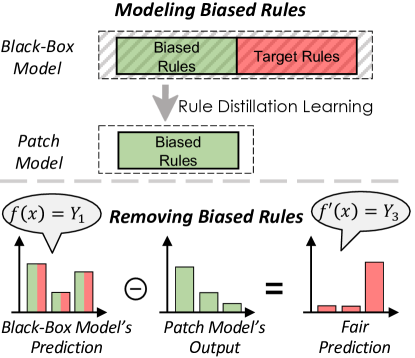
Figure 1: Illustration of the proposed Eraser. In the Distill stage, biased rules are distilled and imparted to the patch model. In the Remove stage, the bias response extracted by the patch model is removed from the model output.

Inference-Time Rule Eraser, by removing model rules from model output, accomplishes the debiasing of deployed models. Extensive experimental evaluations demonstrate that Eraser has superior debiasing performance for deployed models, even outperforming those methods that incorporate fairness constraints into the training algorithm for retraining. Furthermore, While Eraser’s primary focus is on fairness issues, its effectiveness in addressing general bias concerns has also been validated. This highlights the adaptability and practicality of Eraser in addressing problems instigated by spurious prediction rules.

The contributions of this paper are summarized as follows:

• We theoretically analyzed and verified the feasibility of removing biased rules and retaining target rules based on model output, without the need for access to model parameters, to obtain unbiased results. Then, our theoretical analysis led to the derivation of Inference-Time Rule Eraser (Eraser), a straightforward yet effective method for eliminating biased rules.

• We further propose Rule Distillation Learning, which employs a small number of queries to distill biased rules from a black-box model. These distilled biased rules are stored in a patch model to capture the responses of biased rules about test samples.

• To the best of our knowledge, we are the first in the field of machine learning, not just limited to fairness, to explicitly edit the predictive rules from the model output without modifying the model parameters.

2 Related Works

This section provides an overview of the most relevant research to our study, including fairness in machine learning, existing model rule editing approaches, and causal intervention.

2.1 Fairness in Machine Learning

Fairness in machine learning (ML) has become a major research focus. Methods for measuring bias, such as Equalodds [10], have revealed that AI models can exhibit societal bias towards specific demographic groups, including gender and race [14, 15]. Strategies to promote fairness can be broadly classified into pre-processing, in-processing, and post-processing methods [16], which correspond to interventions on the training data, the training algorithm, and the trained model, respectively. Among them, in-processing has received the most research attention and has demonstrated the most effective debiasing performance, while post-processing methods have been the least studied.

Pre-processing methods are designed to modify the distribution of training data, making it difficult for the training algorithm to establish a statistical correlation between bias attributes and tasks [17, 18, 19]. For example, study [17] suggests adjusting the distribution of training data to construct unbiased training data. Another study [18] proposes the generation of new samples to modify the distribution of training data through data augmentation. These strategies aim to decouple the target variable in the training data from the bias variable, thereby preventing the learning of bias in the training of the target task. In-processing methods focus on incorporating additional fairness-aware constraints during ML training [8, 7, 20, 21, 22, 21]. For instance, research [8] introduces adversarial fairness penalty terms, which minimize the learning of features related to bias variables during the learning process of the target task, thereby mitigating bias. Some studies [7, 20] propose fairness-aware contrastive learning loss that brings samples with different protected attributes closer in feature space, thereby reducing differential treatment by the model. Despite their effectiveness, these methods generally do not extend to debiasing deployed models without retraining.

The field of post-processing is primarily concerned with the calibration of pre-trained machine learning models to ensure fairness [11, 12]. A common approach in this area involves adjusting the predictions of models to align with established fairness benchmarks[10, 9]. For instance, some methods modify model outputs directly to satisfy the Equalodds standard by solving an optimization problem [9]. The study by Hardt et al. proposes the learning of distinct classification thresholds for various groups or alterations in output labels to fulfill fairness criteria [10]. However, these techniques necessitate explicit bias labels during testing as the thresholds and output transformation probabilities are group-specific. An alternative approach [23] approximates the impact of fine-tuning models through optimizing parameters added to the model. A study [24] suggests modifying the weight of neurons, identified by causality-based fault localization, to eliminate model bias. Another study [25] employs reweighted features to fine-tune the last layer of parameters, thereby reducing reliance on biased features. However, these methods necessitate modifying model parameters. In addition,  [26] suggests adjusting model predictions by identifying bias in model outputs and modifying protected attributes accordingly, which aids in achieving individual and group fairness standards on tabular data. Nevertheless, this method requires altering protected attributes of test examples during testing, a task that poses challenges for computer vision data. Recent research introduces a pixel perturbation network that adds extra pixel perturbations to the input image to minimize bias [11, 12]. However, this method requires additional access to the model’s parameters to perform gradient backpropagation for training the perturbation network.

Our approach diverges from existing post-processing methods as we view the biased rules in the model as rules that can be removed. We investigate a method for model rule editing that relies solely on model output, without requiring access to model parameters or any labels of test samples. This novel approach allows us to systematically and flexibly eliminate bias in black-box models.

2.2 Rule Editing

Rule Editing [27] provides a lightweight approach to modifying the rules or knowledge embedded in pre-trained models, bypassing the need for full retraining. Existing methods for Rule Editing can be broadly classified into three categories: model fine-tuning, local parameter modification, and structural expansion.

Model fine-tuning is a straightforward approach to rule editing. It involves using data that complies with the desired rules to fine-tune the model. For instance, some studies [28] fine-tune pre-trained language models to correct inaccuracies in their knowledge, significantly reducing the computational costs compared to retraining. Other research [29] suggests further reducing costs by adjusting eigenvalues after performing singular value decomposition (SVD) on the backbone network. Research [27] proposes generating counterfactuals for erroneous rules in training data and using them for fine-tuning to correct the model’s rules. Local parameter modification [30, 24, 31] focuses on adjusting specific model parameters related to the rules to be edited. These methods first identify the relevant parameters by comparing neuron activation differences between rule-aligned and rule-conflicting samples, then retrain these parameters. In addition to fine-tuning the identified local parameters, other research [32] proposes directly reversing the neural activation encoded by the located parameters without training. Structural expansion is another approach to address model editing. Research [33] leverages the properties of ReLU and proposes a theoretically guaranteed repair technique.

However, these rule editing techniques require adjustments to the structure or parameter weights of white-box models, presenting challenges when editing rules in black-box scenarios. In contrast, the Eraser method we propose only requires modifying the model’s output to indirectly edit its rules, providing a more flexible approach for black-box models.

2.3 Causal Inference

Causal inference, as established by Pearl [13], has been a cornerstone in various disciplines such as economics, politics, and epidemiology for many years [34, 35, 36]. Recently, it has gained considerable interest within the machine learning community. Causal inference not only provides an interpretive framework that uncovers the inherent causal relationships within models, but it also guides the elimination of spurious associations, thereby revealing the desired model effects through the pursuit of genuine causal relationships. In recent years, causal inference has been successfully applied to computer vision to eliminate confounding effects caused by dataset confounders in domain-specific applications, such as visual question answering [37], visual common sense reasoning [38], object grounding [39], and long-tailed visual recognition [40]. Causal intervention, a key aspect of causal inference, aims to sever the association between parent and child nodes that may have a confounding effect by intervening child nodes with external forces. This practice is represented as do operation. However, not all scenarios can use do operation to forcibly sever the association between nodes. For instance, in medical experiments, we cannot use a do operation to forcibly modify patients into a population with certain diseases. Backdoor adjustment [41] provides an indirect way to perform do operations and is one of the most widely used implementations of causal intervention. For example, research [42, 43] utilizes causal intervention to eliminate confounding factors in small-sample classification and weakly supervised segmentation. Other research [44] has employed causal intervention to train feature extractors with common sense knowledge. Unlike these existing works that apply causal inference to guide training during the training stage, our work applies causal inference to an already-trained black-box model, to eliminate the influence of confounder (target) rules in the model output and solely distill pure biased rules.

3 Inference-Time Rule Eraser

In this section, we take a close look at the deployed model from the perspective of Bayesian inference, focusing on the manifestation patterns of biased rules within the model output. We then introduce Inference-Time Rule Eraser, a flexible method conceived from an output probabilistic standpoint, aimed at removing biased rules from the model’s output without necessitating any alterations to the model parameters.

3.1 Problem Formulation

The problem of debiasing deployed models can be formally defined as follows: Given an already-trained deployed model, denoted as $\mathcal{M}_{\theta}$ with model parameters $\theta$, which has been trained on a large dataset $\mathcal{D}_{L}$. This model $\mathcal{M}_{\theta}$ serves as a black-box machine learning service that takes an input $x\in\mathbb{X}$ and produces an output $\mathcal{M}_{\theta}(x)$. The training dataset $\mathcal{D}_{L}$ and the model parameters $\theta$ are inaccessible. To perform debiasing on $\mathcal{M}_{\theta}$, we are provided with a small-scale dataset called the calibration dataset $\mathcal{D}_{S}=\{\mathbf{x}_{i},y_{i},b_{i}\}_{i=1:N},|\mathcal{D}_{S}|\ll|\mathcal{D}_{L}|$. Here $\mathbf{x}_{i}\in\mathcal{X}_{S}$ denotes the $i^{th}$ input feature, $y_{i}\in\mathbb{Y}$ denotes its target label, $b_{i}\in\mathbb{B}$ denotes its bias label, and $|\mathcal{D}_{S}|\ll|\mathcal{D}_{L}|$ represents the size of $\mathcal{D}_{S}$ is significantly smaller than the training set of the deployed model $\mathcal{D}_{L}$. Under the premise of not modifying the model parameters $\theta$, the goal of debiasing for deployed models is to achieve unbiased outputs that exclusively respond to the target rules within the model $\mathcal{M}_{\theta}$, devoid of any influence from biased rules.

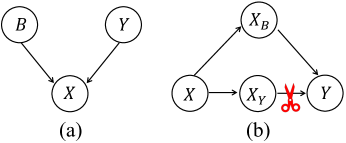
Figure 2: The causal graph. (a) The generation process of data $X$. (b) The inference process of the biased model, where input $X$ produces output $Y$. The red scissor symbolizes the causal intervention we impose.

3.1.1 Bayesian Inference

The issue of fairness fundamentally involves two variables: the target variable $Y$ and the bias variable $B$. Both variables shape the generation of data $X$, as demonstrated in Fig. 2(a). For instance, image data $x$ may contain both the target feature $x_{y}$ (i.e., the feature representing the target variable $y$) and the bias feature $x_{b}$ (i.e., the feature representing the bias variable $b$, such as gender).

Fair machine learning models should base predictions of $y$ exclusively on the target feature $x_{y}$ of the input $x$. However, the inherent nature of machine learning is to learn all features that are beneficial for optimizing the likelihood $p(y|x)$. In the biased training dataset that has a high correlation between the target variable and the bias variable, i.e., the prior $p(y|b)$ is imbalanced, machine learning models often tend to make decisions based on bias features $x_{b}$ of the input $x$, which causes the model to be biased.

Bayesian Inference of Biased Models.    In machine learning, we are generally interested in estimating the conditional probability $p(y|x)$. From a Bayesian perspective, the conditional probability $p(y|x)$ of biased models can be interpreted as:

$$p(y=j|x)=p(y=j|x,b)=\frac{p(x|y=j,b)}{p(x|b)}p(y|b),$$ (1)

where the conditional probability $p(y|x)$ can be expressed as $p(y|x,b)$. This is because, although $b$ is not directly fed into the model, it can be regarded as an implicit input due to its impact on the generation process of $x$, as illustrated in Fig. 2(a). The probabilities $p(y|b)$ and $p(x|b)$ represent the unknown data distribution of the biased model’s training set $\mathcal{D}_{L}$.

Bayesian Inference of Fair Models.    Fair machine learning models, on the other hand, aim to rely solely on target features $x_{t}$ strive to optimize the model towards a fair data distribution, denoted as $\hat{p}(x,y,b)$. This distribution maintains a uniform correlation between $y$ and $b$, i.e., $\hat{p}(y|b)=1/k$, where $k$ is the number of classes in the target variable. This uniform correlation indicates that there is no statistical association between $y$ and $b$. For $\hat{p}(x,y,b)$, the conditional probability of $y$ given $x$, denoted as $\hat{p}(y=j|x)$, can be decomposed using Bayesian interpretation:

$$\hat{p}(y=j|x)=\hat{p}(y=j|x,b)=\frac{\hat{p}(x|y=j,b)}{\hat{p}(x|b)}\hat{p}(y|b),$$ (2)

$$\hat{p}(y|b)=1/k.$$

The reason $\hat{p}(y|b)=1/k$ is because fair machine learning aims to optimize towards a data distribution where the target variable $y$ and bias variable $b$ are independent of each other. These modeling requirements of fair machine learning can be observed in fairness metrics such as Equalodds [10].

Assuming that all instances in the training dataset of the biased model and the fair data distribution are generated from the same process $p(x|y,b)$, i.e., $p(x|y,b)=\hat{p}(x|y,b)$, there can still be a discrepancy between the training set of biased models and the fair data distribution due to differences in the conditional distribution $p(y|b)$ and evidence $p(x|b)$. This discrepancy in the two Bayesian interpretations reflects the influence of the bias rule in the biased model. By eliminating the difference in the two Bayesian interpretations while retaining the learning of biased models for $p(x|y,b)$, we can remove the biased rule from the biased model and retain the target rule. To achieve this, we introduce the Inference-Time Rule Eraser in the following section.

3.2 Inference-Time Rule Eraser

In machine learning, the model’s inference for input sample $x$ is essentially an estimation of the conditional probability $p(y|x)$. This conditional probability can be modeled as a multinomial distribution $\phi$:

$$\phi=\phi_{1}^{\mathbf{1}\{y=1\}}\phi_{2}^{\mathbf{1}\{y=2\}}\cdots\phi_{k}^{\mathbf{1}\{y=k\}};$$ (3)

$$\quad\phi_{j}=\frac{e^{\eta_{j}}}{\sum_{i=1}^{k}e^{\eta_{i}}};\quad\sum_{j=1}^{k}\phi_{j}=1$$

where $\mathbf{1}\{\cdot\}$ denotes the indicator function. The Softmax function maps the model’s class-$j$ logits output, denoted as $\eta_{j}$, to the conditional probability $\phi_{j}$.

From a Bayesian inference perspective, $\phi_{j}$ can be interpreted according to the Bayes theorem as presented in Eq. 1. To distinguish between the outputs of biased models and fair models, we use $\eta_{j}$ and $\phi_{j}$ to represent the logit for class-$j$ and conditional probability $p(y=j|x)$ for biased models’ outputs, respectively. Similarly, we use $\hat{\eta}_{j}$ and $\hat{\phi}_{j}$ to represent the logit for class-$j$ and conditional probability $\hat{p}(y=j|x)$ for fair models’ outputs, respectively.

To remove bias rule and retain only the target rule in the outputs, we introduce the Inference-Time Rule Eraser:

Theorem 1.

(Inference-Time Rule Eraser) Assume $\hat{\phi}$ to be the conditional probability of the fair models that without bias rule, with the form $\hat{\phi}_{j}=\hat{p}(y=j|x)=\hat{p}(y=j|x)=\frac{p(x|y=j)}{{p}(x)}\frac{1}{k}$, and $\phi$ to be the conditional probability of the biased (deployed) model that with bias rule, with the form $\phi_{j}=p(y=j|x)=\frac{p(x|y=j)}{p(x)}\frac{n_{j}}{\sum_{i=1}^{k}n_{i}}$. If $\phi$ is expressed by the standard Softmax function of model output $\eta$, then $\hat{\phi}$ can be expressed as

$$\hat{\phi_{j}}=\frac{e^{log(\phi_{j})-log(p(y=j|b))}}{\sum_{i=1}^{k}e^{log(\phi_{i})-log(p(y=i|b))}}$$ (4)

Proof. The conditional probability of a categorical distribution can be parameterized as an exponential family. It gives us a standard Softmax function as an inverse parameter mapping:

$$\quad\phi_{j}=\frac{e^{\eta_{j}}}{\sum_{i=1}^{k}e^{\eta_{i}}},\quad\hat{\phi_{j}}=\frac{e^{\hat{\eta_{j}}}}{\sum_{i=1}^{k}e^{\hat{\eta_{i}}}}$$ (5)

and also the canonical link function:

$$\eta_{j}=\log\frac{\phi_{j}}{\phi_{k}},\hat{\eta}_{j}=\log\frac{\hat{\phi}_{j}}{\hat{\phi}_{k}}$$ (6)

Given that all instances in the data distribution of biased models and fair models are generated from the same process $p(x|y,b)$, i.e., $p(x|y,b)=\hat{p}(x|y,b)$. Thus we can combine Equ. 1 and Equ. 2:

$$\hat{\phi}_{j}=\phi_{j}\cdot\frac{p(y=j|b)}{\hat{p}(y=j|b)}\cdot\frac{\hat{p}(x|b)}{p(x|b)}$$ (7)

where $\hat{p}(y=j|b)=1/K$.

Subsequently, we apply Equ. 7 to Equ. 6:

$$\hat{\eta}_{j}=\log\frac{\phi_{j}\cdot p(y=j|b)\cdot K\cdot\hat{p}(x|b)}{\hat{\phi}_{k}\cdot p(x|b)}$$ (8)

Then, combining Eqn.  and Eqn. , we have:

$$\hat{\phi_{j}}=\frac{e^{\eta_{j}-\log p(y=j|b)-\log\frac{p(x|b)}{k\cdot\hat{p}(x|b)}}}{\sum_{i=1}^{k}e^{\eta_{i}-\log p(y=i|b)-\log\frac{p(x|b)}{k\cdot\hat{p}(x|b)}}}=\frac{e^{\eta_{j}-\log p(y=j|b)}}{\sum_{i=1}^{k}e^{\eta_{i}-\log p(y=i|b)}}$$ (9)

and since $\eta_{j}=\log\frac{\phi_{j}}{\phi_{k}}$, we have:

$$\hat{\phi_{j}}=\frac{e^{log(\phi_{j})-log(Pr(y=j|b))}}{\sum_{i=1}^{k}e^{log(\phi_{i})-log(Pr(y=i|b))}}$$ (10)

Theorem 1 (Inference-Time Rule Eraser) shows that debiasing deployed models can be accomplished through adjustments to the model output. It proposes that the influence of biased decision rules $p(y|b)$ can be removed by subtracting them in logarithmic ($log$) space from the model outputs, enabling debiasing without requiring access to the model parameters. While the Inference-Time Rule Eraser indeed illuminated the path towards debiasing for deployed models, deriving $p(y|b)$ from the unknown training data distribution of the deployed model presents a challenge due to our lack of access to these data distributions. Essentially, the deployed model is a parameterized representation of the conditional probability $p(y|x)$ in training data distribution. Given that the bias feature about $b$ is a component of $x$, as illustrated by the generation process in Fig. 2(a), the deployed model implicitly models $p(y|b)$. The deployed model’s ability to receive inputs and produce outputs offers us a potential solution to this problem. In the following section, we will explore how to obtain $p(y|b)$ from the deployed model and apply the Inference-Time Rule Eraser.

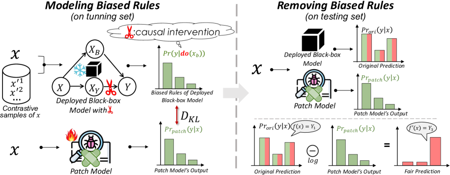
Figure 3: The debiasing performance and the capability to uncover bias under different degrees of data balance ($\alpha$). Larger $\alpha$ indicates that the training set is more balanced.

4 The Proposed Implementation

4.1 Overview

The Inference-Time Rule Eraser mitigates bias in deployed models by removing the bias rule $p(y|b)$ from the log space of the model’s output. However, obtaining $p(y|b)$ from the deployed model during inference is a challenge, which is a prerequisite for the Inference-Time Rule Eraser. This difficulty arises because the model’s behavior can only be understood through its outputs for specific input queries, which contain mixed rules rather than isolated biased rules $p(y|b)$.

To address this challenge, we propose a rule distillation learning approach. This method involves extracting the bias rule from the deployed model by leveraging concepts from causal inference and learning it into a supplementary small model called a patch model. This patch model can process input test samples $x$ to generate outputs reflecting pure biased rules $p(y|b)$. Consequently, as illustrated in Figure X, the complete bias mitigation method consists of two stages, both involving the patch model as an intermediary: (1) In the preparation stage, rule distillation learning is applied to extract pure biased rules from the deployed model and transfer them to the patch model, as explained in Section 4.2. (2) In the bias rule removal stage, the trained patch model provides $p(y|b)$ to adjust the original outputs of test samples, following the Inference-Time Rule Eraser method to eliminate biased rules. This process will be introduced in Sec. 4.3.

4.2 Rule Distillation learning

To obtain the response of the bias rule $p(y|b)$ of the deployed model for test samples, a straightforward idea is to create an additional model that purely encapsulates the bias rule of the deployed model and obtain its response for test samples. For this purpose, we suggest Rule Distillation learning which aims to distill the bias rule from the deployed model and learn it into a small-scale model, referred to as a patch model. This patch model is designed to accept test samples x as input and generate the bias rule response $p(y|b)$. We will elaborate on the distillation and learning aspects of Rule Distillation learning in the following.

Rule Distillation    We begin by visiting the causal relationship between the input feature $x\in X$ and model output $y\in Y$ within the deployed model. The causal graph of the inference process of the deployed model is represented in Figure XX(a), where the model’s output $y\in Y$ relies on both features $x_{y}\in X_{Y}$ pertaining to target label $y\in Y$ and features $x_{b}\in X_{B}$ associated with bias label $b\in B$ in input $x\in X$. Here, $X_{B}\rightarrow Y$ represents the contribution of bias information to the target output $p(y|x_{b})$, where $p(y|x_{b})$ is equivalent to $p(y|b)$ because the deployed model’s use of bias information b can only be through $x_{b}$. For subsequent bias removal, $p(y|x_{b})$ is of interest. However, since $x_{t}$ acts as a confounder creating the backdoor path (confounding effect) $x_{t}\rightarrow y$ to $x_{b}\rightarrow y$, our direct observation of the deployed model’s output y is a blend of two paths rather than purely the path $x_{b}\rightarrow y$, i.e., $p(y|x_{b})$.

We address this issue by providing only $x_{b}$ to the model and not including $x_{t}$, which interrupts the backdoor path from $x_{t}$ to $y$. In particular, given the challenge of editing samples in non-tabular data, we use contrasting sample pairs to interpolate at the representation layer, simulating the state of only supplying $x_{b}$ to the model. Our strategy is driven by the intriguing observation made by recent work showing that the features deep in a network are usually linearized [45, 46]. As shown in Figure xx, taking a target class number K=2 as an example, there exists a semantic direction in the deep feature space, i.e., the model’s representation layer $h(\cdot)$, such that moving a data sample along this direction in the feature space results in a feature representation corresponding to another sample with a different target label but the same bias label. As such, we propose translating the sample’s representation $h(x)$ along this direction until the sample is no longer close to any target class. The translated representation is denoted as $h(\overline{x})$, which is in a state of maximum uncertainty regarding target class information and will only contain information about $x_{b}$.

Given that this direction is not known, we locate a sample $x\prime$ in the dataset for the sample $x$ that shares the same bias label but has a different target label. We then calculate:

$$h(\overline{x})=\frac{1}{k}(h(x)+h(x\prime)$$ (11)

where $h(\overline{x})$ does not lean towards any particular target class and exhibits maximum uncertainty regarding the target class. Similarly, this can be generalized to situations where the target class number K¿2:

$$~{}h(\overline{x})=\frac{1}{K}(h(x)+\sum_{x\prime\in J(x)}h(x\prime)$$ (12)

where $J(x)$ represents the contrastive set about $x$ searched from the $\mathcal{D}_{S}$. There exist $K-1$ samples in $J(x)$, each of which shares the same bias attribute as $x$, but has a different target label from $x$, and the target labels of samples in J$(x)$ are also different from each other.

For deployed models $\mathcal{M}_{\theta}$, $p(y|x_{b})$ is the result of $h(\overline{x})$ after passing through the linear classifier $f(\cdot)$ stacked on top of it and the softmax mapping:

$$p(y|b)$$ (13)

$$=p(y|x_{b})$$

$$=softmax(f(h(\overline{x})))$$

$$=softmax(f(\frac{1}{K}(h(x)+\sum_{x\prime\in J(x)}h(x\prime)))$$

$$=softmax(\frac{1}{K}(f(h(x))+\sum_{x\prime\in J(x)}f(h(x\prime)))$$

Due to the canonical link function, Then:

$$p(y|x_{b})=softmax(\frac{1}{K}log\mathcal{M}_{\theta}(x)+\sum_{x\prime\in J(x)}log(\mathcal{M}_{\theta}(x\prime)))$$ (14)

Hence, we don’t require access to the model parameters. By just obtaining the model’s output for the sample $x$ and its contrast sample $x\prime$, we can derive $p(y|x_{b})$, i.e. p(y—b). We formal this process as follows:

Proposition 1.

Given a model $\mathcal{M}_{\theta}$, a sample $x$, and a sample set $J(x)$, where $|J(x)|=K-1$. If for $\forall x_{i},x_{j}\in J(x)\cup{x}$, $x_{i}$ and $x_{j}$ have the same bias attributes but different target attributes, then the bias rule in model $\mathcal{M}_{\theta}$ regarding to $x$ can be approximately computed as $softmax(\frac{1}{K}log\mathcal{M}_{\theta}(x)+\sum_{x\prime\in J(x)}log(\mathcal{M}_{\theta}(x\prime)))$.

Although our proposition appears heuristic, it is readily proven by the theory of causal intervention. Causal intervention [13] aims to eliminate the confusion caused by confounding factors on the desired causal relationship. In our problem, causal intervention is applicable for eliminating confusion brought about by information $X_{T}$ on the causal relationship $p(y|x_{b})$ between modeling $x_{b}$ and $y$. As depicted in causal graph 5.4(b), to remove the causal relationship $X_{Y}\rightarrow Y$, the causal relationship $X_{B}\rightarrow Y$, i.e., $P(y|do(x_{b}))$ can be modeled by severing $X\rightarrow X_{B}$ using the do operation based on causal intervention. Backdoor adjustment, a specific method of do, deliberately forces $X_{B}$ to fairly incorporate every $x_{t}$, subject to its prior $p(x_{y})$ rather than being subject to spurious correlation between $x_{t}$ and $x_{b}$, into Y’s prediction:

$$p(y\mid do(x_{b}))=\sum_{x_{y}}p(y\mid x_{b},x_{y})p(x_{y})$$ (15)

Due to the NWGM linear approximation of softmax proved in [47]:

$$p(y\mid do(x_{b}))\approx p(y\mid x_{b},\sum_{x_{y}}x_{y}\cdot p(x_{y}))$$ (16)

where $x_{y}$ is a continuous variable, but we can discretize it into $k=k$ different values according to the target label, and $p(x_{y})=1/K$ represents that it follows a normal distribution:

$$p(y\mid do(x_{b}))\approx p(y\mid x_{b},\sum_{i=1}^{K}x_{y}^{y=i}\cdot\frac{1}{K})$$ (17)

where $\sum_{i=1}^{K}x_{y}^{y=i}\cdot\frac{1}{K}$ approximates the average of different target features $x_{t}$ corresponding to different target classes in Equ. 12. Hence, Equ. 12 and the subsequent derivations have taken the correct step.

Multiple Contrastive Samples    However, modeling biased rules by constructing sample pairs in Equ. (LABEL:contrastive) is not entirely accurate. For instance, the bias feature $x_{b}$ of the observed sample $x$ and the bias feature $x_{b}^{\prime}$ of the contrastive sample $x\prime$ differ significantly. Furthermore, the conspicuousness of the target feature (whether it is easily distinguishable) is inconsistent. These discrepancies result in the introduction of noise in the biased rules that the patch model learns via Equ (LABEL:distill).

A natural solution to this issue is to observe multiple contrastive samples instead of single ones:

$$p(y|x_{b})=$$ (18)

$$softmax(\frac{1}{K}( log\mathcal{M}_{\theta}(x)+$$

$$\sum_{i=1,i\neq y_{x}}^{K}\frac{1}{|S_{y=i,b=b_{x}}|}\sum_{x_{s}\in S_{y=i,b=b_{x}}}log(\mathcal{M}_{\theta}(x_{s})))$$

where $y_{x}$ and $b_{x}$ denote the target label and bias label of the sample $x$, respectively, and $S_{y=i,b=b_{x}}$ represents the subset of samples that have a target label of $i$ and a bias label of $b_{x}$. By observing a sample set $S_{y=i,b=b_{x}}$ for each target class, this avoids the noise brought about by merely observing a single sample in Equ.x.

Rule Learning    The rule distillation method outlined in the preceding section necessitates the availability of sample label information. However, this information is not accessible for test samples during the application phase. To obtain biased rules about the test sample during the application phase without any label knowledge about the test sample, we propose the use of an additional patch model, which we refer to as the patch mode, $\mathcal{P}_{\theta}$, to store the biased rules $p(y|x_{b})$ that we have distilled from the deployed model. This enables $\mathcal{P}_{\theta}$ to directly provide the biased rules for the test sample during the application phase.

Using the small-scale dataset $\mathcal{D}_{S}$ that is used for rule removal, we employ the biased rules $p(y|x_{b})$ about x, distilled from the deployed model, as soft labels. Then, we minimize the KL distance $\mathcal{D}_{KL}$ between the output of the patch model and soft labels to store biased rules into patch models:

$$\mathcal{P}_{\theta}=\underset{\mathcal{P}_{\theta}}{\operatorname{argmin}}\mathcal{D}_{KL}\left(\mathcal{P}_{\theta}(x)\,\|\,p\left(y|do(x_{b})\right)\right)$$ (19)

Group-wise Normalization    In the training process of the patch model, each sample possesses its distinct soft labels. Given the small scale of the dataset DS, samples with similar features of interest may have varying soft labels, potentially disrupting the stability of the patch model training. To alleviate this instability, we introduce Group-wise Normalization as follows:

$$\mathcal{P}_{\theta}^{+}=\underset{\mathcal{P}_{\theta}}{\operatorname{argmin}}\mathcal{D}_{KL}\left(\mathcal{P}_{\theta}(x)\,\|\,\frac{1}{|G|}\sum_{x^{g}\in G}p\left(y|do(x^{g}_{b})\right)\right)$$ (20)

where $G$ denotes the set of samples that have the same target label and bias label as $x$. By averaging the original soft labels of the samples in the set $G$ as the final soft label, we normalize the optimization objective of similar samples for the learning of the patch model. On an experimental basis, we demonstrate that the proposed normalization mitigates the instability of the patch model.

4.3 Rule Removing

Our ultimate goal is to obviate the use of biased rules during model inference. As discussed in the previous section, the patch model has learned the biased rules, $P(y|xb)$, distilled from the deployed black-box model. Consequently, the patch model’s response to the input sample x, $\mathcal{P}_{\theta}(x)$, can take the place of $Pr(y|xb)$ in the Fair Bayesian Repair formula (5.10), as depicted in Figure 5.3.

During the testing stage, we utilize the output from the patch model to rectify the bias present in the deployed black-box model:

$$Pr_{repair}(y=j|x)=\frac{e^{log(\phi_{j})-log(Pr_{patch}(t=j|x))}}{\sum_{i=1}^{k}e^{log(\phi_{i})-log(\mathcal{P}_{\theta}(x))}}$$ (21)

where $Pr_{repair}(y=j|x)$ is the final fair output, adjusted from the original output of the biased black box model. $\phi$ is the original probabilistic output of the black box model, and $\mathcal{P}_{\theta}(x)$ is the probabilistic output of the patch model.

As elucidated by the above equation, the proposed debiasing method for deployed models negates the need for any modification to the parameters of the deployed model. During the testing phase, it merely necessitates the subtraction of the patch model’s output from the probabilistic output of the original black box model, within the log space.

5 Experience

This section presents the experimental results of RuleEraser. We begin by introducing the setup, which includes the evaluation metrics, 8 datasets, baseline methods for comparison, and implementation details. Following this, we present results on existing datasets and our ImageNet-B, which is built based on the industrial-scale dataset, ImageNet [48]. While our experiments are primarily focused on vision tasks, we stress that the core concept and methodology are not limited to them and can efficiently debiasing in structured datasets. Furthermore, we extensively analyze the robustness of our method to the data volume of repair data and model structure, along with an ablation study. Finally, we explore the general bias removal capability of our method, using backdoor elimination as a case study.

5.1 Setup

5.1.1 Points of comparison

In experience, we aim to answer two main questions: (1) How does the performance of models, corrected by RuleEraser, compare with other methods? (2) How does the fairness of these models? To answer the first question, we divide the test set into different groups based on target attributes and biased attributes, and test accuracy on each group, and then report the average group accuracy and the worst group accuracy. To answer the second question, we examine whether the model predictions meet the fairness criterion Equalodds, which measures the changes in model predictions when the biased attributes shift. For example, in blonde (T=0) and non-blonde (T=1) hair color recognition, EqualOdds measures gender bias as follows:

$$\frac{1}{|T|}\sum_{t}\left|\operatorname{Acc}_{\text{group}(T=t,B=b^{0})}-\operatorname{Acc}_{\text{group}(T=t,B=b^{1})}\right|$$ (22)

where $T$ denotes target labels, $B$ denotes bias attributes such as male ($b^{0}$) and female ($b^{1}$). $\operatorname{Acc}_{\text{group}(T=t,B=b^{0})}$ represents the accuracy of the group $T=t,B=b^{0}$ in the test set.

5.1.2 Datasets

We evaluate our method against the baselines across 7 different datasets to ensure comprehensive coverage of various debiasing tasks. Seven of these datasets have been proposed in previous research and include both visual and tabular data. However, given the lack of datasets related to multi-class problems in industrial-scale data, we have additionally constructed ImageNet-B to test the debiasing performance.

CelebA [49] is a large-scale face image recognition dataset comprising 200,000 images, containing 40 attributes for each image, of which Gender is the bias attribute that should be prevented from being uesed for prediction. We chose Attractive, Bignose, and Blonde as target attributes for three recognition tasks to verify our gender debiasing effect, as they exhibit the highest Pearson correlation with gender. UTKface [50] is a dataset that contains around 20k facial images annotated with ethnicity, gender, and age. It is used to validate ethnicity debiasing performance by constructing a biased training set with gender and age as target attributes. Although fairness research typically focuses on binary classification tasks, multi-class scenarios are more practical. Therefore, we also used multi-class dataset Colored-MNIST [51] to evaluate debiasing. Colored-MNIST is a dataset of handwritten digits (0-9) with different background colors, where each digit has a strong correlation with the background color. Debiasing aims to eliminate the spurious dependency on background color information in the digit recognition task. Considering the simplicity of the patterns in Colored-MNIST, we constructed an industrial-scale biased dataset, ImageNet-B(ias), based on the ImageNet [48] to validate debiasing performance on complex data. The details of ImageNet-B will be elucidated later. In addition, we are interested in investigating the debiasing effect of our method when multiple biases coexist. The UrbanCar dataset [52] presents a unique opportunity as it encompasses two bias attributes: background (bg) and co-occurring object (co-obj), with the target attribute being the type of car urban, country. This dataset was constructed by segmenting and subsequently recombining images from three distinct datasets: Stanford Cars [53] for car images, Places [54] for background images, and LVIS [55] for images of co-occurring objects.

In addition to the aforementioned visual datasets, we also evaluated debiasing techniques on two structured/tabular datasets, namely LSAC [56] and COMPAS [57], both of which are extensively utilized in fairness literature. Specifically, we examined the performance of race debiasing in the context of law school admission prediction for LSAC, and in recidivism prediction for COMPAS.

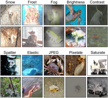
Figure 4: Illustration of majority (95$\%$) samples in ten superclasses in ImageNet-B(ias) dataset.

The construction details of the ImageNet-B(ias) dataset.   Since there exists no off-the-shelf industrial-scale dataset specially designed to analyze the debiasing performance in multi-classification tasks, we propose ImageNet-B(ias), a dataset to facilitate the study of debiasing in complex tasks. Specifically, we utilize ten types of natural noise patterns [58] as bias attributes, including fog, snow, and brightness, among others. We then group semantically similar classes from ImageNet into ten super-classes, derived from WordNet [59], to serve as target attributes. Finally, 95$\%$ of images from each super-class are assigned a a specific type of natural noises, while the remaining 5$\%$ of images are randomly assigned one of the other nine types of noises. As a result, each super-class demonstrates a strong correlation with a specific type of natural noise, as illustrated in Figure 4. For instance, the majority of samples in the super-class of cats predominantly exhibit frost noise.

5.1.3 Baselines

To evaluate the effectiveness of Eraser in debiasing for deployed models, we examined its performance on a range of deployed models with different extents of unfairness. We trained three types of models to serve as the deployed models: the vanilla model, the fair model, and the unfair model. Specifically, (1) The vanilla model was trained using cross-entropy loss without the application of any debiasing technique. (2) The fair model was developed by integrating a constraint about fairness into the model optimization objective. There are two typical methods: AdvDebias, which incorporates fairness-related adversarial regularization terms in the loss function [8]; and ConDebias, which leverages contrastive learning to eradicate bias attribute information from the representation [7, 51]. (3) The unfair model was trained to have the classification ability of both target attributes and bias attributes via multi-task learning [60], thereby further extracting bias features. Furthermore, if we do not consider the specific conditions and resources available during the debiasing process, there are also some methods for debiasing after model training. However, these methods necessitate access to bias labels of test samples or model parameters, requirements not needed by our method. We compared our method with these methods under laboratory conditions, i.e., all conditions required by these methods are met, such as model parameters can be modified. These methods include: (1) Equalodds: Solving a linear program to find probabilities with which to change output labels to optimize equalized odds [10], (2) CalEqualodds: Optimizing over calibrated classifier score outputs to find probabilities with which to change output labels with an equalized odds objective [9], (3) FAAP: Applying perturbations to input images to pollute bias information in the images [11], (4) Repro: Adding learnable padding to all images to optimize the model output to satisfy fairness metrics [12], (5) CARE: Modifying the weight of neurons, identified by causality-based fault localization, to eliminate model bias [24], (6) DFR: Employing reweighted features to fine-tune the last layer of parameters to eliminate the reliance on biased features [25]. Among these, Equalodds and CalEqualodds require known bias labels of test samples. FAAP and Repro need to obtain the model’s gradients by accessing the model’s parameters. CARE and DFR need to modify the weight of partial parameters in the model.

5.1.4 Implementation details

To investigate the debiasing effect on the deployed models, we initially pre-train deployed models. For each target task, we employ four methods (as detailed in Sec. 5.1.3) to train the deployed models, leveraging 60$\%$ of the data from each respective dataset. The backbone of the models is set by default as ResNet-34 [61]. To demonstrate the robustness of our method to the architecture of deployed models, we also employ the ViT-B/32 [62] Transformer as the backbone. The remaining 20$\%$ of the data in each dataset is then used for learning how to debias, such as training the patch model in our method. Subsequently, the remaining 20$\%$ of the data in each dataset is utilized for learning how to debias, such as training the patch model in our method. To be as lightweight as possible, our patch model selects the smaller ResNet-18 [61] as its backbone. Finally, the last 20$\%$ of the dataset is used for testing.

5.2 Quantitative Results

5.2.1 Main Debiasing performance

Table I presents the quantitative results, including accuracy and model bias, of deployed models before and after being embedded with the proposed Eraser on four datasets. For the CelebA dataset, we utilize three commonly used target tasks (refer to Table I(a) to I(c)) for gender debiasing evaluation. For the UTKFace dataset, we evaluate ethnicity debiasing (see Table I(d)). For multi-class datasets, namely C-MNIST and our constructed ImageNet-B, we examined background color debiasing and natural noise debiasing respectively (refer to Table I(e) and I(f)).

For the CelebA and UTKFace datasets, two types of fair training (AdvDebias and ConDebias) can yield a model that is fairer than the Vanilla model, i.e., lower model bias (Equalodds), due to the incorporation of fairness constraints. Not surprisingly, unfair training results in a model that is less fair than the Vanilla. For all four types of models, after applying our method, they consistently show a significant improvement in fairness (reduction in model bias) and an increase in accuracy. The main observations include: (1) For the Vanilla models, after applying our method, the model bias is reduced by more than 70$\%$, reaching up to 89$\%$ at most. For example, in the Attractive task, the model bias is reduced from 20.92 to 2.30. Accompanied by the reduction in model bias, average and worst group accuracy also increase, from 76.85 to 78.76 and from 66.20 to 75.73, respectively. (2) For the two types of fair models, AdvDebias and ConDebias, our method can further improve the fairness and accuracy of these models. For example, for the AdvDebias models in Blonde task, our method still improves fairness (model bias reduction from 11.12 to 5.35) and improves accuracy (from 85.07 to 90.31 and from 61.72 to 85.34 in average and worst group accuracy, respectively). This indicates that our method is compatible with the fairness constraints in training. (3) For unfair model, Eraser can significantly improve its fairness and accuracy. For instance, in the BigNose task, Eraser can decrease model bias to 3.34, while improving average group accuracy to 72.92. (4) Also, given that our method is limited to not modifying model parameters, debiasing during training is more straightforward than our method. However, a comparison of our method versus debiasing during training in Table I reveals that a vanilla model integrated with our method can achieve almost superior fairness and accuracy performance than a model that underwent fair training (e.g., Vanilla model+FAAP has even better accuracy and model bias than Fair model (AdvDebias and ConDebias) in I(a)). This comparison further demonstrates the potential of our method.

For the multi-class datasets, C-MNIST and our constructed ImageNet-B, we present the debiasing performance in Table I(e) and Table I(f), respectively. Similar observations to CelebA and UTKface can be obtained. After the application of our method, four diverse types of deployed models consistently show significant improvements in both accuracy and fairness. This suggests that our method is not confined to binary tasks, which are the current focus of fairness research, but is applicable to more complex multi-class tasks. Furthermore, the debiasing performance on ImageNet-B also attests to the applicability of our method to datasets of industrial magnitude.

TABLE I: Results of deployed models before and after integration with the proposed Eraser on CelebA (Table I(a) to I(c)), UTKFace (Table I(d)), C-MNIST ( Table I(e)) and ImangeNet-B (Table I(f)). For target task performance, we report average group accuracy (in $\%$, $\uparrow$) and Worst group accuracy (in $\%$, $\uparrow$). For model bias, we report Equalodds (in $\%$, $\downarrow$).

CelebA, BigNose	Average ACC $\uparrow$	Worst ACC $\uparrow$	Model Bias $\downarrow$
Vanilla model	69.48$\pm$0.2	36.45$\pm$0.6	23.26$\pm$0.3
Vanilla model + Eraser	75.14$\pm$0.2	71.52$\pm$0.5	3.72$\pm$0.2
Fair model (AdvDebias)	68.41$\pm$0.4	36.21$\pm$0.8	12.59$\pm$0.5
Fair model + Eraser	72.93$\pm$0.4	60.12$\pm$0.5	4.59$\pm$0.4
Fair model (ConDebias)	72.96$\pm$0.2	53.04$\pm$0.6	8.59$\pm$0.5
Fair model + Eraser	75.52$\pm$0.4	72.54$\pm$0.5	6.01$\pm$0.4
Unfair model	69.89$\pm$1.0	42.20$\pm$1.7	20.70$\pm$1.4
Unfair model + Eraser	72.92$\pm$0.7	66.85$\pm$1.0	3.34$\pm$0.7

(a) Results on CelebA when the target label is BigNose

UTKFace	Average ACC $\uparrow$	Worst ACC $\uparrow$	Model Bias $\downarrow$
Vanilla model	86.59$\pm$0.4	72.61$\pm$0.4	18.28$\pm$0.3
Vanilla model + Eraser	90.09$\pm$0.3	85.03$\pm$0.4	5.40$\pm$0.3
Fair model (AdvDebias)	87.91$\pm$1.2	75.62$\pm$1.9	10.82$\pm$1.5
Fair model + Eraser	88.85$\pm$1.0	86.03$\pm$1.4	4.36$\pm$1.1
Fair model (ConDebias)	86.23$\pm$1.0	76.45$\pm$1.5	10.57$\pm$1.3
Fair model + Eraser	88.64$\pm$0.6	85.36$\pm$0.8	6.20$\pm$0.6
Unfair model	84.41$\pm$0.7	70.41$\pm$1.1	22.14$\pm$0.8
Unfair model + Eraser	88.03$\pm$0.5	82.45$\pm$0.9	3.05$\pm$0.6

(d) Results on UTK-face with ethnicity as the bias attribute

CelebA, Blonde	Average ACC $\uparrow$	Worst ACC $\uparrow$	Model Bias $\downarrow$
Vanilla model	82.39$\pm$0.3	46.13$\pm$0.7	22.06$\pm$0.6
Vanilla model + Eraser	91.54$\pm$0.3	85.64$\pm$0.5	6.24$\pm$0.3
Fair model (AdvDebias)	85.07$\pm$0.5	61.72$\pm$0.9	11.12$\pm$0.6
Fair model + Eraser	90.31$\pm$0.5	85.34$\pm$0.7	5.35$\pm$0.7
Fair model (ConDebias)	82.46$\pm$0.3	55.05$\pm$0.7	13.63$\pm$0.4
Fair model + Eraser	90.46$\pm$0.2	80.33$\pm$0.6	5.94$\pm$0.3
Unfair model	80.45$\pm$1.3	38.93$\pm$1.4	25.51$\pm$1.3
Unfair model + Eraser	92.21$\pm$0.7	88.35$\pm$0.8	4.71$\pm$0.8

(b) Results on CelebA when the target label is Blonde

C-MNIST	Average ACC $\uparrow$	Worst ACC $\uparrow$	Model Bias $\downarrow$
Vanilla model	77.90$\pm$0.3	12.91$\pm$2.1	14.46$\pm$1.3
Vanilla model + Eraser	95.88$\pm$0.3	76.35$\pm$1.3	2.50$\pm$0.3
Fair model (AdvDebias)	94.35$\pm$0.3	19.54$\pm$1.7	3.79$\pm$0.8
Fair model + Eraser	96.58$\pm$0.4	74.95$\pm$1.1	2.38$\pm$0.3
Fair model (ConDebias)	96.32$\pm$0.4	89.12$\pm$2.0	2.08$\pm$0.7
Fair model + Eraser	96.45$\pm$0.3	89.88$\pm$1.4	1.77$\pm$0.3
Unfair model	73.65$\pm$0.9	11.90$\pm$2.2	18.65$\pm$1.4
Unfair model + Eraser	94.86$\pm$0.4	57.08$\pm$0.8	3.20$\pm$0.3

(e) Results on Colored-MNIST with background color as the bias attribute

CelebA, Attractive	Average ACC $\uparrow$	Worst ACC $\uparrow$	Model Bias $\downarrow$
Vanilla model	76.85$\pm$0.4	66.20$\pm$0.7	20.92$\pm$0.4
Vanilla model + Eraser	78.76$\pm$0.4	75.73$\pm$0.6	2.30$\pm$0.4
Fair model (AdvDebias)	80.25$\pm$0.7	74.13$\pm$1.3	7.01$\pm$0.9
Fair model + Eraser	80.33$\pm$0.5	76.24$\pm$0.7	5.92$\pm$0.7
Fair model (ConDebias)	78.82$\pm$0.8	72.00$\pm$0.9	11.70$\pm$0.8
Fair model + Eraser	79.78$\pm$0.5	76.23$\pm$0.7	1.45$\pm$0.5
Unfair model	76.45$\pm$1.0	64.74$\pm$1.3	20.13$\pm$1.1
Unfair model + Eraser	78.28$\pm$0.6	77.43$\pm$0.7	1.01$\pm$0.6

(c) Results on CelebA when the target label is Attractive

ImageNet-B	Average ACC $\uparrow$	Worst ACC $\uparrow$	Model Bias $\downarrow$
Vanilla model	61.24$\pm$0.3	26.01$\pm$0.9	13.84$\pm$0.4
Vanilla model + Eraser	75.33$\pm$0.3	49.63$\pm$0.5	6.47$\pm$0.3
Fair model (AdvDebias)	64.51$\pm$0.6	29.38$\pm$0.8	10.62$\pm$0.4
Fair model + Eraser	68.48$\pm$0.2	43.79$\pm$0.5	6.54$\pm$0.2
Fair model (ConDebias)	63.26$\pm$0.4	28.03$\pm$1.0	10.27$\pm$0.7
Fair model + Eraser	67.68$\pm$0.3	42.05$\pm$0.7	6.96$\pm$0.4
UnFair model	56.34$\pm$0.4	18.02$\pm$1.1	15.24$\pm$0.3
UnFair model + Eraser	71.82$\pm$0.5	46.87$\pm$0.6	6.83$\pm$0.3

(f) Results on ImageNet-B with natural noise as the bias attribute

TABLE II: Results of deployed models, both before and after integration with the proposed Eraser, on structured datasets LSAC and COMPAS.

Method		LSAC					COMPAS
		Average ACC $\uparrow$	Worst ACC $\uparrow$	Model Bias $\downarrow$			Average ACC $\uparrow$	Worst ACC $\uparrow$	Model Bias $\downarrow$
Vanilla model		64.44 $\pm$0.5	19.02 $\pm$1.3	26.48 $\pm$0.8			62.35 $\pm$0.6	45.47 $\pm$1.5	19.45 $\pm$0.9
Vanilla model+Eraser		69.01 $\pm$0.6	57.04 $\pm$0.9	4.11 $\pm$0.7			63.59 $\pm$0.4	58.43 $\pm$0.6	2.03 $\pm$0.5
Fair model (AdvDebias)		65.73 $\pm$0.9	46.35 $\pm$1.7	10.59 $\pm$1.3			54.49 $\pm$0.8	41.72 $\pm$1.6	14.78 $\pm$1.2
Fair model+Eraser		69.31 $\pm$0.6	58.61 $\pm$1.0	4.23 $\pm$0.7			59.45 $\pm$0.4	58.32 $\pm$0.9	2.87 $\pm$0.6
Fair model (ConDebias)		64.51 $\pm$1.2	43.82 $\pm$1.6	12.31 $\pm$1.3			59.98 $\pm$0.8	40.45 $\pm$1.4	4.28 $\pm$1.2
Fair model+Eraser		68.66 $\pm$0.6	56.81 $\pm$0.7	3.80 $\pm$0.6			62.97 $\pm$0.6	58.31 $\pm$0.7	2.65 $\pm$0.6
Unfair model		63.60 $\pm$1.4	17.01 $\pm$2.3	29.98 $\pm$1.9			61.38 $\pm$1.2	31.30 $\pm$2.0	38.07 $\pm$1.5
Unfair model+Eraser		66.75 $\pm$0.7	60.92 $\pm$0.8	4.96 $\pm$0.7			62.92 $\pm$0.7	61.82 $\pm$0.9	2.01 $\pm$0.8

5.2.2 Results on structured data.

To demonstrate the versatility of our proposed method, we extended our experimentation beyond image data to include structured datasets. Table II showcases the debiasing performance on two structured datasets, LSAC and COMPAS, both of which are extensively utilized in fairness studies. By integrating our Eraser with the vanilla model, we consistently achieved a marked increase in fairness and accuracy on both datasets. For example, on LSAC dataset, the model bias is reduced from 20.92 to 2.30. Accompanied by the reduction in model bias, average and worst group accuracy increase from 64.44 to 69.01 and from 19.02 to 57.04, respectively. In addition, our method performs consistently on structured datasets with its performance on image datasets, is also compatible with the fair model and can further enhance its fairness and accuracy. Moreover, in line with previous observations, the performance of vanilla model when combined with our method surpasses that of standalone fair models, highlighting the remarkable debiasing capability of our method. These findings on structured datasets indicate that our method is not limited to specific data types or patterns, but is broadly applicable to both images and structured data.

5.2.3 Debiasing with multiple biases.

In the realm of machine learning, it is not uncommon for multiple biases to be present in the training data of deployed models. These biases often find their way into the deployed model, leading to biased predictions. We performed experiments to gauge the effectiveness of our method in simultaneously eliminating multiple biases in a single deployed model. We conducted experiments on the Urbancars dataset, which concurrently exhibits both background (BG) bias and co-occurring object (Co-obj) bias. Initially, we pre-trained the deployed model on the Urbancars dataset using four different training methods. Subsequently, for each deployed model, our method trains two patch models, patch-BG and patch-Co-obj, to counteract the BG and Co-obj biases in the deployed model, respectively. To mitigate multiple biases, we merge the two patch models to debias at the same time, referred to as Eraser${}_{\text{\,BG + o-obj}}$. The final output after debiasing can be formalized as:

$$\frac{e^{log(\phi_{j})-log(Pr_{\text{patch-BG}}(t=j|x))-log(Pr_{\text{patch-Co-obj}}(t=j|x))}}{\sum_{i=1}^{k}e^{log(\phi_{i})-log(Pr_{\text{patch-BG}}(t=i|x))-log(Pr_{\text{patch-Co-obj}}(t=i|x))}}$$ (23)

where the symbols have the same meaning as in Equ 21.

As indicated in Table III, when Eraser${}_{\text{\,bg + co-obj}}$ is used to mitigate the two biases, both biases decreases markedly. For example, for the vanilla model, BG bias reduction from 32.07 to 4.84 and Co-obj bias reduction from 28.01 to 3.25. This suggests that our method can be stacked to reduce multiple biases, making it more suitable for more complex multi-bias scenarios.

TABLE III: Debiasing results for multi-biases on UrbanCars dataset. We report background (BG) bias, co-occurring object (Co-obj) bias, and the average of BG bias and Co-obj bias.

	Method	Accuracy		Model Bias
		Average ACC$\uparrow$	Worst ACC$\uparrow$	BG Bias$\downarrow$	Co-obj Bias$\downarrow$	Avg Bias$\downarrow$
	Vanilla model	77.27 $\pm$0.6	28.05 $\pm$1.4	32.07 $\pm$1.3	28.01 $\pm$2.2	30.04 $\pm$1.6
	Vanilla model + Eraser${}_{\text{\,BG + Co-obj}}$	86.63 $\pm$0.7	77.82 $\pm$1.1	4.84 $\pm$1.2	3.25 $\pm$0.9	4.05 $\pm$0.6
	Fair model (AdvDebias)	82.13 $\pm$1.3	62.42 $\pm$2.5	19.36 $\pm$1.7	10.77 $\pm$1.9	15.06 $\pm$1.8
	Fair model + Eraser${}_{\text{\,BG + Co-obj}}$	86.44 $\pm$0.9	76.56 $\pm$2.1	4.70 $\pm$0.6	3.12 $\pm$0.7	3.91 $\pm$0.7
	Fair model (ConDebias)	84.74 $\pm$1.1	67.25 $\pm$3.4	20.64 $\pm$1.8	8.56 $\pm$1.6	14.6 $\pm$1.7
	Fair model + Eraser${}_{\text{\,BG + Co-obj}}$	87.39 $\pm$0.7	77.62 $\pm$1.2	5.02 $\pm$1.4	4.64 $\pm$0.8	4.83 $\pm$1.2
	Unfair model	75.26 $\pm$1.6	17.62 $\pm$3.1	33.67 $\pm$1.1	38.45 $\pm$2.9	36.06 $\pm$1.9
Car Object	Unfair model + Eraser${}_{\text{\,BG + Co-obj}}$	85.40 $\pm$0.9	67.26 $\pm$1.3	1.20 $\pm$1.4	4.38 $\pm$0.3	2.79 $\pm$0.9

TABLE IV: Debiasing results of different post-training debiasing methods on six tasks under laboratory conditions. The best results are highlighted in bold. The second-best results are underlined. The Equalodds and CalEqualodds are not suitable for multi-classification tasks (indicated by “-”).

	CelebA,BigNose			CelebA,Blonde			CelebA,Attractive			UTKFace			C-MNIST			ImageNe-B
Methods	Avg. ACC $\uparrow$	Worst ACC $\uparrow$	Model Bias $\downarrow$	Avg. ACC $\uparrow$	Worst ACC $\uparrow$	Model Bias $\downarrow$	Avg. ACC $\uparrow$	Worst ACC $\uparrow$	Model Bias $\downarrow$	Avg. ACC $\uparrow$	Worst ACC $\uparrow$	Model Bias $\downarrow$	Avg. ACC $\uparrow$	Worst ACC $\uparrow$	Model Bias $\downarrow$	Avg. ACC $\uparrow$	Worst ACC $\uparrow$	Model Bias $\downarrow$
Vanilla	$69.48$	$36.45$	$23.26$	$82.39$	$46.13$	$22.06$	$76.85$	$66.20$	$20.92$	$86.59$	$72.61$	$18.28$	$77.90$	$12.91$	$14.46$	$61.24$	$26.01$	$13.84$
Equalodds	$64.95$	$42.23$	$\bf{1.50}$	$71.86$	$45.12$	$\bf{0.70}$	$71.74$	$\underline{71.21}$	$\bf{1.06}$	$80.59$	$73.14$	$\bf{1.67}$	$-$	$-$	$-$	$-$	$-$	$-$
CalEqualodds	$57.87$	$36.45$	$20.62$	$68.48$	$29.36$	$8.62$	$77.51$	$69.20$	$16.49$	$76.08$	$42.43$	$17.39$	$-$	$-$	$-$	$-$	$-$	$-$
FAAP	$\underline{72.82}$	$46.74$	$6.97$	$86.98$	$66.45$	$5.24$	$77.76$	$67.23$	$8.26$	$\underline{88.12}$	$\underline{78.13}$	$9.27$	$84.67$	$\underline{36.57}$	$\underline{4.95}$	$\underline{73.67}$	$\underline{44.29}$	$7.89$
Repro	$70.35$	$47.53$	$9.23$	$84.49$	$60.04$	$11.04$	$78.04$	$64.31$	$11.13$	$87.12$	$77.62$	$10.28$	$81.49$	$25.17$	$8.27$	$72.51$	$42.31$	$9.57$
CARE	$71.53$	$46.96$	$19.79$	$86.97$	$77.59$	$13.58$	$\underline{78.53}$	$68.79$	$19.87$	$87.61$	$77.79$	$13.92$	$86.07$	$20.45$	$7.90$	$72.59$	$41.63$	$7.56$
DFR	$70.15$	$\underline{47.64}$	$20.83$	$\underline{89.49}$	$\underline{78.35}$	$12.25$	$77.61$	$68.39$	$18.34$	$87.98$	$78.05$	$11.05$	$\underline{86.43}$	$21.56$	$7.61$	$72.62$	$42.85$	$\underline{7.39}$
Eraser	$\bf{75.14}$	$\bf{71.52}$	$\underline{3.72}$	$\bf{91.54}$	$\bf{85.64}$	$\underline{6.24}$	$\bf{78.76}$	$\bf{75.73}$	$\underline{2.30}$	$\bf{90.09}$	$\bf{85.03}$	$\underline{5.40}$	$\bf{95.88}$	$\bf{76.35}$	$\bf{2.50}$	$\bf{75.33}$	$\bf{49.63}$	$\bf{6.47}$

5.3 Qualitative Evaluation

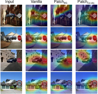
Figure 5: Grad-CAM results of the deployed model and two patch models on UrbanCars dataset.

In our quest to provide a comprehensive understanding of our method, we incorporate the model explanation approach Grad-CAM [63] to illustrate our learned patch model successfully captures the bias present in the deployed model. This is a crucial aspect as it directly influences the efficiency of bias removal from the deployed model using the patch model. For a more granular analysis, we chose the UrbanCars dataset, which is known to contain both types of biases. In Fig. 8, we present attention maps of the deployed model and two patch models, which are designed to capture background (BG) bias and co-occurring object (Co-obj) bias, respectively. It is evident that the deployed model’s focus extends beyond the areas containing cars to include the BG and Co-obj (e.g., traffic signs) areas. The two patch models we trained are focused on the BG and Co-obj areas in the image, respectively, as anticipated. This indicates that the patch model precisely replicates the bias in the deployed model, which substantiates why our method can efficiently eradicate bias without a corresponding decrease in accuracy.

5.4 Comparison Under Laboratory Conditions

There exist additional post-training debiasing techniques that, regrettably, require either access to bias labels of test samples or model parameters. This requisite poses a significant constraint in practical, real-world scenarios. To offer a more comprehensive evaluation of our method, we compared our method with these methods in a controlled laboratory setting, i.e., all conditions required by these methods are met. Table IV presents the quantitative results on image data, where Vanilla represents the deployed model requiring debiasing. Our proposed method exhibits outstanding performance in terms of both fairness and accuracy across all six tasks. Take the Attractive recognition task as an example. The vanilla models exhibit substantial fairness issues (model bias = 20.92), with the average group accuracy being a mere 76.82. However, our proposed Eraser method significantly reduces the model bias to 2.30 and enhances the worst group accuracy to 78.76. Various debiasing techniques exhibit varying degrees of effectiveness in bias alleviation. Different debiasing techniques show varying degrees of effectiveness in bias mitigation. The Equalodds method slightly outperforms our method in terms of fairness (model bias of Equalodds is 1.06 in the Attractive task) but significantly falls behind in average group accuracy (71.74 for Equalodds versus 78.76 for our method). Moreover, the Equalodds model is only applicable to binary classification tasks and is not suitable for multi-classification scenarios. The debiasing capabilities of CARE and DFR are task-dependent. They show limited debiasing performance in the Attractive and BigNose tasks. This could be because the target features and bias features in the deployed model for these tasks are more entangled, making it impossible to achieve debiasing by modifying some parameters. In summary, while our method eliminates the need for additional laboratory conditions, it still achieves state-of-the-art performance when compared to other methods.

5.5 Analysis and discussion

Applicability for scenarios with only little data.    We further investigated the relationship between the amount of data used to train the patch model and the debiasing effect. By merely adjusting the volume of training data for the patch model, the size ratio between the training set of the patch model and the training set of the deployed model was adjusted within a range from 1/1000 to 1/5. A smaller size ratio indicates a smaller amount of data used to train the patch model. For instance, when the size ratio is 1/1000, the data volume is only 160 images. It’s worth noting that there is no overlapping data between the training set of the patch model and the deployed model.

Figure 6 displays the debiasing results at different size ratios. Our method exhibits significant debiasing performance at different size ratios. For example, even when the size ratio is 1/1000, we still achieved a 20$\%$ reduction in bias. Furthermore, the larger the amount of data used to train the patch model (the larger the size ratio), the better the debiasing performance. However, this trend is very weak. For instance, the model bias only differs by 1.3, and the accuracy only differs by 1.3 between size ratios of 1/1000 and 1/5. These results indicate that our proposed Eraser is not sensitive to the amount of data. Even with a very small amount of data (such as only $\sim$ 160 images), our method remains applicable, demonstrating the high practicality of our approach.

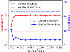
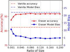
Figure 6: Debiasing performance when using different sizes of data.

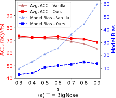
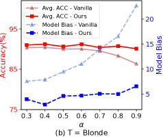
Figure 7: Debiasing performance for deployed models with varying levels of model bias, where different deployed models are trained with data of different bias levels; a larger $\alpha$ indicates a higher degree of data bias.

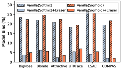
Figure 8: Debiasing performance on deployed models using different probability evaluation functions.

Robustness to Bias Severity in Deployed Models   In real-world scenarios, varying degrees of data imbalance have the potential to introduce biases in deployed models. To assess the effectiveness and robustness of our proposed in debiasing deployed models derived from different levels of data bias, we initially created datasets with diverse degrees of data imbalance using the CelebA dataset. The level of data imbalance, controlled by the $\alpha$, signifies the ratio between the number of minority class samples and majority class samples (with biased labels distinct from the minority class), where a smaller $\alpha$ indicates a higher degree of data imbalance. Subsequently, we trained different deployed models using these datasets with different $\alpha$, and assessed the capability of our approach to mitigate biases in these deployed models.

Figure 4 provides a comprehensive analysis of the relationship among accuracy, model bias, and the data bias level $\alpha$ on the CelebA dataset, focusing on the Attractive target task. As $\alpha$ decreases, the deployed models learn more severe biases. By applying our proposed approach to these diverse deployed models, significant reductions in bias and improvements in accuracy are achieved across all models. Importantly, these improvements are consistent and do not deteriorate as $\alpha$ decreases.

The probability evaluation functions of deployed models.    Our method is derived based on Bayesian analysis. Therefore, it is fundamentally independent of the probability evaluation functions used by the deployed model, despite the theoretical derivation using the softmax probability distribution as an example.

To verify this claim, we present the debiasing results of the deployed model using sigmoid as the probability evaluation function, comparing them with the results obtained when using softmax, in Fig.9. It is evident that our method exhibits consistent bias reduction performance for both the deployed model using softmax and the deployed model using sigmoid. This demonstrates the notion that our approach is independent of the specific choice of probability evaluation functions used in the deployed model and is applicable to sigmoid, not limited to softmax.

TABLE V: Effect of backbone architectures in BigNose on CelebA dataset.

Backbone	Method	Avg. Acc ($\uparrow$)	Worst Acc ($\uparrow$)	Model Bias ($\downarrow$)
Resnet-34	Vanilla	69.48±0.2	36.45±0.6	23.26±0.3
	Eraser	75.14±0.2	71.52±0.5	3.72±0.2
VIT-B/32	Vanilla	60.01±0.1	11.75±0.6	27.53±0.3
	Eraser	66.85±0.1	63.91±0.4	3.75±0.2

Robustness to Network Architectures.    To evaluate the robustness of our method to different backbones of the deployed model, we report its performance using both ResNet-34 [61] and VIT-B/32 [62] as backbones of the deployed model in Table 5. The results demonstrate that our method performs similarly on both Convolutional network and Transformer architectures, two mainstream network architectures, indicating that our method is not sensitive to the model architectures.

6 Conclusion

This paper introduced the Inference-Time Rule Eraser (Rule Eraser), a novel approach to fairness in AI systems. Unlike existing methods, Rule Eraser does not require access to or modification of model weights. It operates by removing biased rules at inference-time, which is achieved by modifying the model’s output. We also proposed a specific implementation, Distill and Remove, which distills biased rules into an additional patched model and removes them during inference time. Our experiments demonstrated the effectiveness and superior performance of Rule Eraser. It also showed broad applicability, with successful validation on model repair problems beyond fairness. This represents a significant advancement in the pursuit of fairness in AI systems, making fairness more accessible in real-world applications.

References

- [1] S. Gong, X. Liu, and A. K. Jain, “Mitigating face recognition bias via group adaptive classifier,” in Proceedings of the IEEE/CVF Conference on Computer Vision and Pattern Recognition (CVPR), June 2021, pp. 3414–3424.
- [2] J. Carpenter, “Google’s algorithm shows prestigious job ads to men, but not to women,” The Independent, vol. 7, 2015.
- [3] J. Dastin, “Amazon scraps secret ai recruiting tool that showed bias against women,” in Ethics of data and analytics. Auerbach Publications, 2022, pp. 296–299.
- [4] M. Raghavan, S. Barocas, J. Kleinberg, and K. Levy, “Mitigating bias in algorithmic hiring: Evaluating claims and practices,” in Proceedings of the 2020 conference on fairness, accountability, and transparency, 2020, pp. 469–481.
- [5] J. Dressel and H. Farid, “The accuracy, fairness, and limits of predicting recidivism,” Science advances, vol. 4, no. 1, p. eaao5580, 2018.
- [6] J. Buolamwini and T. Gebru, “Gender shades: Intersectional accuracy disparities in commercial gender classification,” in Conference on fairness, accountability and transparency. PMLR, 2018, pp. 77–91.
- [7] S. Park, J. Lee, P. Lee, S. Hwang, D. Kim, and H. Byun, “Fair contrastive learning for facial attribute classification,” in Proceedings of the IEEE/CVF Conference on Computer Vision and Pattern Recognition, 2022, pp. 10 389–10 398.
- [8] T. Wang, J. Zhao, M. Yatskar, K.-W. Chang, and V. Ordonez, “Balanced datasets are not enough: Estimating and mitigating gender bias in deep image representations,” in Proceedings of the IEEE/CVF international conference on computer vision, 2019, pp. 5310–5319.
- [9] G. Pleiss, M. Raghavan, F. Wu, J. Kleinberg, and K. Q. Weinberger, “On fairness and calibration,” Advances in neural information processing systems, vol. 30, 2017.
- [10] M. Hardt, E. Price, and N. Srebro, “Equality of opportunity in supervised learning,” Advances in neural information processing systems, vol. 29, 2016.
- [11] Z. Wang, X. Dong, H. Xue, Z. Zhang, W. Chiu, T. Wei, and K. Ren, “Fairness-aware adversarial perturbation towards bias mitigation for deployed deep models,” in Proceedings of the IEEE/CVF Conference on Computer Vision and Pattern Recognition, 2022, pp. 10 379–10 388.
- [12] G. Zhang, Y. Zhang, Y. Zhang, W. Fan, Q. Li, S. Liu, and S. Chang, “Fairness reprogramming,” Advances in Neural Information Processing Systems, vol. 35, pp. 34 347–34 362, 2022.
- [13] J. Pearl, M. Glymour, and N. P. Jewell, Causal inference in statistics: A primer. John Wiley & Sons, 2016.
- [14] S. Yao and B. Huang, “Beyond parity: Fairness objectives for collaborative filtering,” Advances in neural information processing systems, vol. 30, 2017.
- [15] J. Zhao, T. Wang, M. Yatskar, V. Ordonez, and K.-W. Chang, “Men also like shopping: Reducing gender bias amplification using corpus-level constraints,” arXiv preprint arXiv:1707.09457, 2017.
- [16] S. Caton and C. Haas, “Fairness in machine learning: A survey,” ACM Computing Surveys, 2020.
- [17] F. Kamiran and T. Calders, “Data preprocessing techniques for classification without discrimination,” Knowledge and information systems, vol. 33, no. 1, pp. 1–33, 2012.
- [18] V. V. Ramaswamy, S. S. Kim, and O. Russakovsky, “Fair attribute classification through latent space de-biasing,” in Proceedings of the IEEE/CVF conference on computer vision and pattern recognition, 2021, pp. 9301–9310.
- [19] Y. Zhang and J. Sang, “Towards accuracy-fairness paradox: Adversarial example-based data augmentation for visual debiasing,” in Proceedings of the 28th ACM International Conference on Multimedia, 2020, pp. 4346–4354.
- [20] E. Tartaglione, C. A. Barbano, and M. Grangetto, “End: Entangling and disentangling deep representations for bias correction,” in Proceedings of the IEEE/CVF conference on computer vision and pattern recognition, 2021, pp. 13 508–13 517.
- [21] S. Park, S. Hwang, D. Kim, and H. Byun, “Learning disentangled representation for fair facial attribute classification via fairness-aware information alignment,” in Proceedings of the AAAI Conference on Artificial Intelligence, vol. 35, no. 3, 2021, pp. 2403–2411.
- [22] Z. Wang, K. Qinami, I. C. Karakozis, K. Genova, P. Nair, K. Hata, and O. Russakovsky, “Towards fairness in visual recognition: Effective strategies for bias mitigation,” in Proceedings of the IEEE/CVF conference on computer vision and pattern recognition, 2020, pp. 8919–8928.
- [23] M. P. Kim, A. Ghorbani, and J. Zou, “Multiaccuracy: Black-box post-processing for fairness in classification,” in Proceedings of the 2019 AAAI/ACM Conference on AI, Ethics, and Society, 2019, pp. 247–254.
- [24] B. Sun, J. Sun, L. H. Pham, and J. Shi, “Causality-based neural network repair,” in Proceedings of the 44th International Conference on Software Engineering, 2022, pp. 338–349.
- [25] P. Kirichenko, P. Izmailov, and A. G. Wilson, “Last layer re-training is sufficient for robustness to spurious correlations,” in The Eleventh International Conference on Learning Representations, ICLR 2023, Kigali, Rwanda, May 1-5, 2023. OpenReview.net, 2023.
- [26] P. K. Lohia, K. N. Ramamurthy, M. Bhide, D. Saha, K. R. Varshney, and R. Puri, “Bias mitigation post-processing for individual and group fairness,” in Icassp 2019-2019 ieee international conference on acoustics, speech and signal processing (icassp). IEEE, 2019, pp. 2847–2851.
- [27] S. Santurkar, D. Tsipras, M. Elango, D. Bau, A. Torralba, and A. Madry, “Editing a classifier by rewriting its prediction rules,” Advances in Neural Information Processing Systems, vol. 34, pp. 23 359–23 373, 2021.
- [28] N. D. Cao, W. Aziz, and I. Titov, “Editing factual knowledge in language models,” Proceedings of the 2021 Conference on Empirical Methods in Natural Language Processing, vol. 6491–6506, 2021.
- [29] Y. Sun, Q. Chen, X. He, J. Wang, H. Feng, J. Han, E. Ding, J. Cheng, Z. Li, and J. Wang, “Singular value fine-tuning: Few-shot segmentation requires few-parameters fine-tuning,” Advances in Neural Information Processing Systems, vol. 35, pp. 37 484–37 496, 2022.
- [30] M. Usman, D. Gopinath, Y. Sun, Y. Noller, and C. S. Păsăreanu, “Nn repair: Constraint-based repair of neural network classifiers,” in Computer Aided Verification: 33rd International Conference, CAV 2021, Virtual Event, July 20–23, 2021, Proceedings, Part I 33. Springer, 2021, pp. 3–25.
- [31] S. Singla and S. Feizi, “Salient imagenet: How to discover spurious features in deep learning?” in International Conference on Learning Representations, 2022. [Online]. Available: https://openreview.net/forum?id=XVPqLyNxSyh
- [32] Y. Zhao, H. Zhu, K. Chen, and S. Zhang, “Ai-lancet: Locating error-inducing neurons to optimize neural networks,” in Proceedings of the 2021 ACM SIGSAC Conference on Computer and Communications Security, 2021, pp. 141–158.
- [33] F. Fu and W. Li, “Sound and complete neural network repair with minimality and locality guarantees,” in International Conference on Learning Representations, 2022.
- [34] J. G. Brown and I. Ayres, “Economic rationales for mediation,” Va. L. Rev., vol. 80, p. 323, 1994.
- [35] L. Keele, “The statistics of causal inference: A view from political methodology,” Political Analysis, vol. 23, no. 3, pp. 313–335, 2015.
- [36] L. Richiardi, R. Bellocco, and D. Zugna, “Mediation analysis in epidemiology: methods, interpretation and bias,” International journal of epidemiology, vol. 42, no. 5, pp. 1511–1519, 2013.
- [37] Y. Niu, K. Tang, H. Zhang, Z. Lu, X.-S. Hua, and J.-R. Wen, “Counterfactual vqa: A cause-effect look at language bias,” in Proceedings of the IEEE/CVF Conference on Computer Vision and Pattern Recognition, 2021, pp. 12 700–12 710.
- [38] X. Zhang, F. Zhang, and C. Xu, “Multi-level counterfactual contrast for visual commonsense reasoning,” in Proceedings of the 29th ACM International Conference on Multimedia, 2021, pp. 1793–1802.
- [39] W. Wang, J. Gao, and C. Xu, “Weakly-supervised video object grounding via causal intervention,” IEEE Transactions on Pattern Analysis and Machine Intelligence, vol. 45, no. 3, pp. 3933–3948, 2022.
- [40] K. Tang, J. Huang, and H. Zhang, “Long-tailed classification by keeping the good and removing the bad momentum causal effect,” Advances in Neural Information Processing Systems, vol. 33, pp. 1513–1524, 2020.
- [41] J. Pearl, “Interpretation and identification of causal mediation.” Psychological methods, vol. 19, no. 4, p. 459, 2014.
- [42] Z. Yue, H. Zhang, Q. Sun, and X.-S. Hua, “Interventional few-shot learning,” Advances in neural information processing systems, vol. 33, pp. 2734–2746, 2020.
- [43] D. Zhang, H. Zhang, J. Tang, X.-S. Hua, and Q. Sun, “Causal intervention for weakly-supervised semantic segmentation,” Advances in Neural Information Processing Systems, vol. 33, pp. 655–666, 2020.
- [44] T. Wang, J. Huang, H. Zhang, and Q. Sun, “Visual commonsense r-cnn,” in Proceedings of the IEEE/CVF Conference on Computer Vision and Pattern Recognition, 2020, pp. 10 760–10 770.
- [45] P. Upchurch, J. Gardner, G. Pleiss, R. Pless, N. Snavely, K. Bala, and K. Weinberger, “Deep feature interpolation for image content changes,” in Proceedings of the IEEE conference on computer vision and pattern recognition, 2017, pp. 7064–7073.
- [46] Y. Bengio, G. Mesnil, Y. Dauphin, and S. Rifai, “Better mixing via deep representations,” in International conference on machine learning. PMLR, 2013, pp. 552–560.
- [47] K. Xu, J. Ba, R. Kiros, K. Cho, A. Courville, R. Salakhudinov, R. Zemel, and Y. Bengio, “Show, attend and tell: Neural image caption generation with visual attention,” in International conference on machine learning. PMLR, 2015, pp. 2048–2057.
- [48] J. Deng, W. Dong, R. Socher, L.-J. Li, K. Li, and L. Fei-Fei, “Imagenet: A large-scale hierarchical image database,” in 2009 IEEE conference on computer vision and pattern recognition. Ieee, 2009, pp. 248–255.
- [49] Z. Liu, P. Luo, X. Wang, and X. Tang, “Deep learning face attributes in the wild,” in Proceedings of the IEEE international conference on computer vision, 2015, pp. 3730–3738.
- [50] Z. Zhang, Y. Song, and H. Qi, “Age progression/regression by conditional adversarial autoencoder,” in Proceedings of the IEEE conference on computer vision and pattern recognition, 2017, pp. 5810–5818.
- [51] Y. Hong and E. Yang, “Unbiased classification through bias-contrastive and bias-balanced learning,” Advances in Neural Information Processing Systems, vol. 34, pp. 26 449–26 461, 2021.
- [52] Z. Li, I. Evtimov, A. Gordo, C. Hazirbas, T. Hassner, C. C. Ferrer, C. Xu, and M. Ibrahim, “A whac-a-mole dilemma: Shortcuts come in multiples where mitigating one amplifies others,” in Proceedings of the IEEE/CVF Conference on Computer Vision and Pattern Recognition, 2023, pp. 20 071–20 082.
- [53] J. Krause, M. Stark, J. Deng, and L. Fei-Fei, “3d object representations for fine-grained categorization,” in Proceedings of the IEEE international conference on computer vision workshops, 2013, pp. 554–561.
- [54] B. Zhou, A. Lapedriza, A. Khosla, A. Oliva, and A. Torralba, “Places: A 10 million image database for scene recognition,” IEEE transactions on pattern analysis and machine intelligence, vol. 40, no. 6, pp. 1452–1464, 2017.
- [55] A. Gupta, P. Dollar, and R. Girshick, “Lvis: A dataset for large vocabulary instance segmentation,” in Proceedings of the IEEE/CVF conference on computer vision and pattern recognition, 2019, pp. 5356–5364.
- [56] L. F. Wightman, “Lsac national longitudinal bar passage study. lsac research report series.” 1998.
- [57] J. Angwin, J. Larson, S. Mattu, and L. Kirchner, “Machine bias,” in Ethics of data and analytics. Auerbach Publications, 2022, pp. 254–264.
- [58] D. Hendrycks and T. Dietterich, “Benchmarking neural network robustness to common corruptions and perturbations,” Proceedings of the International Conference on Learning Representations, 2019.
- [59] C. Fellbaum, “Wordnet,” in Theory and applications of ontology: computer applications. Springer, 2010, pp. 231–243.
- [60] J. Baxter, “A bayesian/information theoretic model of learning to learn via multiple task sampling,” Machine learning, vol. 28, pp. 7–39, 1997.
- [61] K. He, X. Zhang, S. Ren, and J. Sun, “Deep residual learning for image recognition,” in Proceedings of the IEEE conference on computer vision and pattern recognition, 2016, pp. 770–778.
- [62] A. Kolesnikov, A. Dosovitskiy, D. Weissenborn, G. Heigold, J. Uszkoreit, L. Beyer, M. Minderer, M. Dehghani, N. Houlsby, S. Gelly, T. Unterthiner, and X. Zhai, “An image is worth 16x16 words: Transformers for image recognition at scale,” 2021.
- [63] R. R. Selvaraju, M. Cogswell, A. Das, R. Vedantam, D. Parikh, and D. Batra, “Grad-cam: Visual explanations from deep networks via gradient-based localization,” in Proceedings of the IEEE international conference on computer vision, 2017, pp. 618–626.