Exact Modeling of Power Spectrum Multipole through Spherical Fourier-Bessel Basis

Abstract

The three-dimensional galaxy power spectrum is a powerful probe of primordial non-Gaussianity and additional general relativistic effects, which become important on large scales. At the same time, wide-angle (WA) effects due to differing lines-of-sight (LOS) on the curved sky also become important with large angular separation. In this work, we accurately model WA and Doppler effects using the spherical Fourier-Bessel (SFB) formalism, before transforming the result into the commonly used power spectrum multipoles (PSM). This mapping from the SFB power spectrum to PSM represents a new way to non-perturbatively model WA and GR effects present in the PSM, which we validate with log-normal mocks. Moreover, for the first time, we can compute the analytical PSM Gaussian covariance on large scales, exactly including WA-induced mode-couplings, without resorting to any plane-parallel approximations.

Current and upcoming large-scale structure (LSS) surveys such as DESI Aghamousa et al. (2016), Euclid Amendola et al. (2018), and SPHEREx Doré et al. (2014) will measure the galaxy density field over increasingly larger volume, offering improved constraining power on effects that manifest on large scales, such as the primordial non-Gaussianity (PNG) Komatsu and Spergel (2001); Dalal et al. (2008); Slosar et al. (2008); de Putter and Doré (2017); Rezaie et al. (2023) and general relativistic (GR) effects Yoo et al. (2009); Yoo (2010); Challinor and Lewis (2011); Bonvin and Durrer (2011); Jeong et al. (2012); Elkhashab et al. (2022). With wider angular coverage, the commonly used global plane-parallel approximation, which assumes the same line-of-sight (LOS) for all galaxy pairs, breaks down when the galaxy separation becomes large, and wide-angle (WA) effects become important. Additionally, the Newtonian approximation to redshift space distortion (RSD)– an effect that arise from our measuring the redshifts and not the distances of galaxies – also breaks down as GR effects become important on large scales.

The next best thing to the global plane-parallel approximation is a local one in which each galaxy pair is allowed to have a different LOS. This is achieved by the Yamamoto estimator for measuring the Fourier-space power spectrum multipoles (PSM). An efficient implementation of this is to choose one of the galaxy to be the pair LOS, called the end-point LOS Bianchi et al. (2015); Scoccimarro (2015); Beutler et al. (2019). The signal picked up by this estimator at large scales includes WA effects that are usually modeled either perturbatively as an expansion in the galaxy pair separation Reimberg et al. (2016); Castorina and White (2018); Beutler et al. (2019); Benabou et al. (2024); Beutler and McDonald (2021); Noorikuhani and Scoccimarro (2023); Paul et al. (2023), or non-perturbatively via an exact calculation of the configuration-space correlation function Tansella et al. (2018); Castorina and Di Dio (2022).

In this Letter, we propose an alternative non-perturbative method for calculating the PSM that employs a natural basis for the curved sky: the spherical Fourier-Bessel (SFB) basis, which was proposed in the 90s Binney and Quinn (1991); Lahav (1993) and has recently gained traction Leistedt et al. (2012); Yoo and Desjacques (2013); Nicola et al. (2014); Lanusse et al. (2015); Samushia (2019); Zhang et al. (2021); Grasshorn Gebhardt and Doré (2021); Khek et al. (2022); Grasshorn Gebhardt and Doré (2023). As the eigenfunctions of the Laplacian in the spherical coordinates, the SFB basis preserves the geometry of the curved sky and naturally models the WA effects. Due to the separation of radial and angular modes in spherical coordinates, one can incorporate Newtonian RSD and GR effects more easily for the SFB power spectrum Yoo and Desjacques (2013); Zhang et al. (2021) than for the PSM Castorina and Di Dio (2022).

Despite these advantages, the SFB power spectrum is a less developed formalism compared to the PSM, especially at the mildly non-linear scales ($k\gtrsim 0.05\,h/{\rm Mpc}$). Its estimator also suffers from an increased computational cost due to the large number of modes, and the fact that one cannot employ fast Fourier-transforms as is often used in Cartesian-based estimators Grasshorn Gebhardt and Doré (2021, 2023).

In this work, we build upon Ref. Castorina and White (2018) and fully develop a mapping from the SFB power spectrum to the PSM, which allows us to take advantage of the strengths in both statistics: on large scales we can exactly model WA and GR effects using the SFB power spectrum, before transforming the result into the PSM, to take advantage of its efficient Yamamoto estimator implementation and better developed small-scale modeling. This mapping represents a new way of non-perturbatively modeling WA effects in the PSM, which we validate using log-normal mocks. Moreover, for the first time we obtain an exact analytic covariance for the PSM, handling off-diagonal mode-couplings due to WA effects in the covariance, without resorting to approximations such as those made in Ref. Wadekar and Scoccimarro (2020). Though formulated in the context of galaxy surveys, our results will also have implications for future wide-field intensity mapping surveys Hall et al. (2013); Liu et al. (2016); Viljoen et al. (2021).

Power Spectrum Multipoles–We first briefly review the SFB formalism. The canonical SFB basis is composed of eigenfunctions of the Laplacian in spherical coordinates, namely the spherical Bessel functions of first kind $j_{\ell}(kx)$ and the spherical harmonics $Y^{*}_{\ell m}(\hat{\mathbb{x}})$. The SFB decomposition of the galaxy density field $\delta(\mathbb{x})$ is then:

$$\delta_{\ell m}(k) =\int_{\mathbb{x}}j_{\ell}(kx)Y^{*}_{\ell m}(\hat{\mathbb{x}})\delta(\mathbb{x})\,.$$ (1)

Here, the angular mode $Y_{\ell m}(\hat{\mathbb{x}})$ and the radial mode $j_{\ell}(kx)$ share the same $\ell$, whereas the generalized SFB (gSFB) decomposition Castorina and White (2018) allows for different $L\neq\ell$:

$$\delta_{\ell m}^{L}(k) =\int_{\mathbb{x}}j_{L}(kx)Y^{*}_{\ell m}(\hat{\mathbb{x}})\delta(\mathbb{x})\,.$$ (2)

They form an over-complete basis, but as we shall see, provide a useful bridge for expressing the PSM in the SFB formalism.

The generalized SFB power spectrum is defined as:

$$\langle\delta_{\ell_{1}m_{1}}^{a}(k_{1})\delta_{\ell_{2}m_{2}}^{b*}(k_{2})\rangle=C_{\ell_{1}}^{ab}(k_{1},k_{2})\delta_{\ell_{1}\ell_{2}}^{K}\delta_{m_{1}m_{2}}^{K}\,,$$ (3)

where $\delta^{K}$ is the Dirac-delta. We use the upper indices $a$ and $b$ to indicate the radial modes and the lower index for the angular mode of the gSFB power spectrum. When $a=b=\ell_{1}$, it reduces to the canonical SFB power spectrum $C_{\ell_{1}}(k_{1},k_{2})$. Note that the SFB power spectra adopt two values of $k$, and we call $k_{1}=k_{2}$ diagonal and $k_{1}\neq k_{2}$ off-diagonal.

In a real survey, the observed field $\delta^{{\rm W}}$ contains the survey window function: $\delta^{{\rm W}}(\mathbb{x})=W(\mathbb{x})\delta(\mathbb{x})$. This breaks the azimuthal symmetry, but we can define the azimuthally averaged quantity

$$C_{\ell}^{ab,{\rm W}}(k_{1},k_{2})\equiv\frac{1}{2\ell+1}\sum_{m}\langle\delta_{\ell m}^{a,{\rm W}}(k_{1})\delta_{\ell m}^{b*,{\rm W}}(k_{2})\rangle\,,$$ (4)

which is now similar in form to Eq. 3.

Now the power spectrum multipoles (PSM) $P_{L}(k)$ are defined as, under the end-point LOS Scoccimarro (2015)

$$P_{L}(k) \equiv\frac{(2L+1)}{I_{22}}\int_{\hat{\mathbf{k}}}\int_{\mathbb{x},\mathbb{x}^{\prime}}e^{-i\mathbf{k}\cdot(\mathbb{x}-\mathbb{x}^{\prime})}$$

$$\qquad\langle\delta(\mathbb{x})\delta(\mathbb{x}^{\prime})\rangle W(\mathbb{x})W(\mathbb{x}^{\prime})\mathcal{L}_{L}(\hat{\mathbb{x}}\cdot\hat{\mathbf{k}})\,,$$ (5)

where $\mathcal{L}_{L}(\hat{\mathbb{x}}\cdot\hat{\mathbf{k}})$ is the Legendre polynomial and $I_{22}\equiv\int_{\mathbb{x}}W(\mathbb{x})^{2}$ is the normalization. Using the plane-wave expansion and evaluating the $\hat{\mathbf{k}}$ integral (see full derivation in the Appendix), we find the relationship between the PSM and the gSFB power spectrum:

$$P_{L}(k) =\frac{(4\pi)^{2}(2L+1)}{I_{22}}\sum_{a,b}i^{-a+b}(2a+1)(2b+1)$$

$$\qquad\begin{pmatrix}a&L&b\\ 0&0&0\end{pmatrix}^{2}C_{b}^{ab,{\rm W}}(k,k)\,.$$ (6)

The above equation was first derived in Ref. Castorina and White (2018). Compared to their expression, our Eq. 6 accounts for the window convolution and is expressed in terms of the gSFB power spectrum (Eq. 4) instead of the gSFB mode (Eq. 2). Going beyond Ref. Castorina and White (2018), we will highlight the theoretical importance of Eq. 6 and, for the first time, enable its use for PSM modeling by developing a method to compute the gSFB power spectrum.

Remarkably, the PS monopole is simply

$$P_{0}(k) =\frac{(4\pi)^{2}}{I_{22}}\sum_{b}(2b+1)C_{b}^{{\rm W}}(k,k)\,,$$ (7)

a sum over all the angular modes of the canonical SFB power spectrum. Note that only the diagonal components of the canonical SFB power spectrum are present. These are the only modes that would exist in a homogeneous and isotropic Universe where there were no redshift evolution and LOS-dependent effects like RSD Grasshorn Gebhardt and Doré (2021). This is exactly what the PS monopole is, an average over the orientation of the Fourier mode ${\bf k}$, and it erases the redshift evolution information by integrating over the redshift bin.

Given the above, we would then expect that the off-diagonal components $C_{b}^{W}(k,k^{\prime})$ would be (partially) brought back for the higher multipoles in $P_{L}$. Indeed, this is achieved through the generalized SFB $C_{b}^{ab,\rm W}(k,k)$, where by construction, the off-diagonal information in $C_{b}^{W}(k,k^{\prime})$ is folded into the extra upper radial indices $a$ and $b$, keeping a single $k$ value.

The double sum in Eq. 6 is also weighted by the Wigner-3$j$ symbols, a result of the PSM being a weighted average over the orientation of ${\bf k}$ by the Legendre polynomials. The resulting triangle condition between $a,b$ and $L$ means that, for the commonly-considered PSM $L=0$ to 4, Eq. 6 is effectively reduced to only to a single sum over $b$ (at most a couple hundred of terms for $k\leq 0.1\,h/{\rm Mpc}$) with few terms in $a$, making it computationally efficient. Since WA terms are naturally contained in the gSFB power spectrum, the mapping in Eq. 6 will offer an exact treatment of WA effects in PSM if we can exactly compute the gSFB.

To compute the window-convolved gSFB power spectrum, we first consider the simplest case of a full-sky window with only radial selection $R(x)$. We use the superscript R to indicate this case. Following Refs. Grasshorn Gebhardt and Doré (2021); Khek et al. (2022); Grasshorn Gebhardt and Doré (2023), the radially-convolved gSFB power spectrum can be written as:

$$C_{\ell}^{ab,{\rm R}}(k_{1},k_{2})\equiv\int_{q}\mathcal{W}_{\ell}^{a}(k_{1},q)\mathcal{W}_{\ell}^{b}(k_{2},q)P_{\rm m,0}(q)\,,$$ (8)

where $P_{\rm m,0}(q)$ is the present-day matter power spectrum, $\mathcal{W}_{\ell}^{a}(k,q)$ is the gSFB kernel defined as

$$\mathcal{W}_{\ell}^{a}(k,q)\equiv\sqrt{\frac{2}{\pi}}q\int_{x}x^{2}j_{a}(kx)R(x)\Delta_{\ell}(q,x)\,,$$ (9)

and $\Delta_{\ell}(k,x(z))$ is the angular projection kernel that would contain effects such as RSD, GR Bonvin and Durrer (2011); Challinor and Lewis (2011); Di Dio et al. (2013) and Fingers-of-god (FoG) effects Khek et al. (2022). On linear scales where the FoG effect is small, and in the Newtonian limit, the angular projection kernel becomes

$$\Delta_{\ell}^{\rm RSD}(k,x)=D(x)\left[b_{\rm g}(x)j_{\ell}(kx)-f(x)j_{\ell}^{\prime\prime}(kx)\right]\,,$$ (10)

where $D$ is the growth factor, $b_{g}$ is the linear galaxy bias, and $f$ is the linear growth rate.

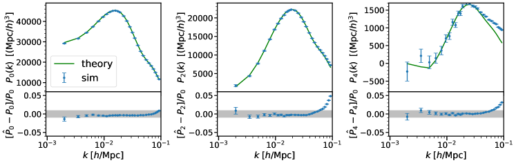
Figure 1: The multipoles $P_{L}(k)$. The green lines show the theoretical results of PSM, and the blue points show the mean and the $1\sigma$ error of the measured multipoles from the 10,000 full-sky mocks for $z=0.2-0.5$. In the lower panels, we show the differences between the measurements and the theoretical results, normalized by the monopole that sets the simulation precision. The grey bands indicate $1\%$ accuracy. Our theoretical results and measurements agree well at large scales.

The integrals in Eq. 8 and 9 can be computed through the procedure introduced in Refs. Khek et al. (2022) and Grasshorn Gebhardt and Doré (2023) where the authors computed the canonical SFB power spectrum. The only change we make is allowing radial and angular modes to have different orders $\ell\neq a$ when computing the gSFB. With this we evaluate the radially-convolved gSFB power spectrum and obtain the PSM using Eq. 6 for an example of the full-sky window (taking $z$ between 0.2 and 0.5). We plot the theory computation for the first five multipoles in solid lines in Fig. 1.

Going beyond the full-sky window, we assume the separability of the window function into angular and radial parts $W(\mathbb{x})=R(x)M(\hat{\mathbb{x}})$. We leave the radial selection $R(x)$ in the gSFB kernel and consider the effects of the angular mask $M(\hat{\mathbb{x}})$. The window-convolved gSFB power spectrum is then:

$$C_{\ell}^{ab,{\rm W}}(k_{1},k_{2})=M_{\ell\ell^{\prime}}C_{\ell^{\prime}}^{ab,{\rm R}}(k_{1},k_{2}),$$ (11)

where $M_{\ell\ell^{\prime}}$ is the angular mode coupling matrix Alonso et al. (2019). This step enables the use of Eq. 6 for realistic surveys.

Validation with Full-sky Mocks– To validate Eq. 6 and showcase its use for modeling WA effects, we compare our theoretical results with measurements from full-sky simulations. In particular, we choose to use the set of log-normal mocks generated in Ref. Benabou et al. (2024). With the goal of studying a perturbative calculation of WA effects, the authors of Ref. Benabou et al. (2024) generated 10,000 full-sky mocks in linear theory with Newtonian RSD, spanning $z=0.2$ to $0.5$. They also provide a new implementation for the following Yamamoto estimator, whose ensemble average is expected to be Eq. 5:

$$\hat{P}_{L}(k)\equiv\frac{(2L+1)}{I_{22}}\int_{\hat{\mathbf{k}}}F_{L}(\mathbf{k})F_{0}(-\mathbf{k})\,,$$ (12)

where

$$F_{L}(\mathbf{k}) \equiv\int_{\mathbb{x}}W(\mathbb{x})e^{-i\mathbf{k}\cdot\mathbb{x}}\mathcal{L}_{L}(\hat{\mathbf{k}}\cdot\hat{\mathbb{x}})\delta(\mathbb{x})\,.$$ (13)

To compare with full-sky mocks under Newtonian RSD, the theoretical modeling of galaxy fluctuation $\delta(\mathbb{x})$ needs to include the canonical Newtonian RSD term, the angular kernel of which is given in Eq. 10. We further need to include an additional velocity contribution scaled with $v/x$, which is generated from the Jacobian associated with the change of coordinates caused by Newtonian RSD Szalay et al. (1998); Pápai and Szapudi (2008); Yoo and Seljak (2015); Raccanelli et al. (2010). This velocity term is usually ignored for mocks or previous surveys with small angular coverage Beutler et al. (2019); Beutler and McDonald (2021); Castorina et al. (2019), but it must be included in the full-sky limit Raccanelli et al. (2010); Benabou et al. (2024). The angular projection kernel corresponding to this velocity term is

$$\Delta^{{\rm v}}_{\ell}(k,x)=-\frac{\alpha(x)}{x}\frac{f(x)}{k}D(x)j_{\ell}^{\prime}(kx)\,$$ (14)

where $\alpha(x)\equiv\partial[\ln x^{2}R(x)]/\partial\ln x$, and it becomes $\alpha=2$ for a uniform radial window in the redshift bin Yoo and Seljak (2015); Castorina and White (2018).

The mocks in Ref. Benabou et al. (2024) are generated with $f=0.71$ and $b_{1}=1.455$, and there is no redshift evolution within the redshift bin for the mocks. All calculations assume a best-fit Planck 2018 cosmology Planck Collaboration VI (2020). The results for the mean of the multipole measurements from the 10,000 mocks with $L$ from 0 to 4 are shown in Fig. 1. We see that our theory predictions agree exceptionally well with the measured multipoles at the largest scales. The disagreements at the small scales ($k\gtrsim 0.06\,h/{\rm Mpc}$) are due to the voxel windows used in the simulations Benabou et al. (2024) which we do not include in our modeling.

Gaussian Covariance– We next express the Gaussian covariance of PSM in terms of the gSFB power spectrum. Compared to Ref. Wadekar and Scoccimarro (2020), which had the state-of-art results for analytical Gaussian covariance of the PSM, we will calculate the exact covariance without resorting to any plane-parallel or LOS approximation. The results in Ref. Wadekar and Scoccimarro (2020) are only applicable in the flat sky limit and on scales where the window function is subdominant, while our expression is exact and can be applied at the largest scales in particular for measuring PNG and GR effects. Using the Yamamoto estimator of Eq. 12, the Gaussian covariance reads Wadekar and Scoccimarro (2020):

$$\textbf{C}^{\textup{G}}_{L_{1}L_{2}}(k_{1},k_{2})=\frac{(2L_{1}+1)(2L_{2}+1)}{I_{22}^{2}}\bigg{[}\int_{\hat{\mathbf{k}}_{1},\hat{\mathbf{k}}_{2}}\langle F_{L_{1}}(\mathbf{k}_{1})F_{0}(-\mathbf{k}_{1})F_{L_{2}}(\mathbf{k}_{2})F_{0}(-\mathbf{k}_{2})\rangle\bigg{]}-\langle\widehat{P}_{L_{1}}(k_{1})\rangle\ \langle\widehat{P}_{L_{2}}(k_{2})\rangle\,.$$ (15)

Using Wick contractions on the 4-point function and expressing $F_{L}(k)$ with Eq. 13, we can follow the same procedure as the PSM case. To simplify the final expression, we further assume the separability of the window function and obtain:

$$\textbf{C}^{\textup{G}}_{L_{1}L_{2}}(k_{1},k_{2})=(4\pi)^{4}\frac{(2L_{1}+1)(2L_{2}+1)}{I_{22}^{2}}\sum_{a,b,c,d,\ell_{1},\ell_{2}}i^{-a-c+b+d}(2a+1)\begin{pmatrix}a&L_{1}&b\\ 0&0&0\end{pmatrix}^{2}\begin{pmatrix}c&L_{2}&d\\ 0&0&0\end{pmatrix}^{2}$$

$$\qquad\Bigg{[}(2c+1)S_{b\ell_{1}d\ell_{2}}+(-1)^{L_{2}}(2d+1)S_{b\ell_{1}c\ell_{2}}\Bigg{]}C_{\ell_{1}}^{ad,{\rm R}}(k_{1},k_{2})C_{\ell_{2}}^{bc,{\rm R}}(k_{1},k_{2})\,,$$ (16)

where we have defined $S_{abcd}$ as the chain of window function (similar to Ref. Grasshorn Gebhardt and Doré (2021)):

$$S_{abcd}\equiv\sum_{m_{a},m_{b},m_{c},m_{d}}M_{am_{a}}^{bm_{b}}M_{bm_{b}}^{cm_{c}}M_{cm_{c}}^{dm_{d}}M_{dm_{d}}^{am_{a}}\,,$$ (17)

and $M_{am_{a}}^{bm_{b}}$ as a double spherical harmonic transform of the angular window $M(\hat{x})$:

$$M_{am_{a}}^{bm_{b}}\equiv\int_{\hat{\mathbb{x}}}M(\hat{\mathbb{x}})Y_{am_{a}}(\hat{\mathbb{x}})Y^{*}_{bm_{b}}(\hat{\mathbb{x}})\,.$$ (18)

Under the separable window assumption, Eq. 16 expressed the PSM covariance as the sum of the product of the radially-convolved gSFB power spectrum. The formula is feasible for numerical computation due to the triangle conditions of the Wigner-3j symbol and $L_{1},L_{2}$ taking only from 0 to 4. In addition, we usually only need to compute covariance once for the cosmological analysis.

Under the full-sky window, the Gaussian auto-covariance of the monopole $\textbf{C}^{\textup{G}}_{00}(k_{1},k_{2})$ simplifies to:

$$\textbf{C}^{\textup{G}}_{00}(k_{1},k_{2}) =\frac{(4\pi)^{4}}{I_{22}^{2}}\sum_{b}2(2b+1)\left[C_{b}^{{\rm R}}(k_{1},k_{2})\right]^{2}\,.$$ (19)

Under the same set-up as our log-normal mocks with full-sky window, we plot an example of the analytical Gaussian covariance matrix using Eqs. 8 and 19 in Fig. 2, which shows prominent off-diagonal components with $k\lessapprox 0.02h/{\rm Mpc}$.

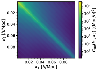
Figure 2: The analytical Gaussian covariance for the PS monopole $\hat{P}_{0}(k)$ evaluated for $z=0.2$ to $0.5$.

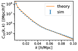
Figure 3: Diagonal elements of the auto-covariance for the monopole $\hat{P}_{0}(k)$ obtained from analytical calculations (orange line, including shot noise) and log-normal mocks (blue points).

Eq. 16 gives the Gaussian covariance for a continuous density field. However, real surveys measure discrete objects (galaxies), which produces a non-negligible shot noise contribution Feldman et al. (1994). To extend Eq. 16 for discrete objects, we can include the shot noise to the gSFB power spectrum following Ref. Grasshorn Gebhardt and Doré (2021), which will then allow validation of analytical covariance with covariance estimated from mocks. We compare the diagonal elements of the auto-covariance for the PS monopole obtained from analytical calculations and log-normal mocks in Fig. 3, and they show good agreement.

Even though the mock-based method of estimating covariance can also include WA effects, it would be computationally expensive to generate a large number of full-sky mocks to achieve the desired accuracy in the covariance. It is also challenging to incorporate GR effects into the mocks, which will require ray-tracing of N-body simulations Borzyszkowski et al. (2017); Lepori et al. (2020) (or even GR N-body simulations Adamek et al. (2016); Bonvin et al. (2023)) of large volumes, so analytical covariance is preferred at large scales. Our result Eq. 16 lays out the foundation for computing exact analytical covariance at the largest scales for upcoming LSS surveys.

Conclusion and discussion– Through Eqs. 6 and 16, the main results of this letter, we have expressed the PSM and its covariance in terms of the generalized SFB power spectrum. The SFB basis naturally incorporates the WA effect present in the PSM without perturbative expansion of galaxy separation. It also provides a new way to do window convolution of the PSM through the SFB basis, without using the effective redshift approximation Castorina et al. (2019); Castorina and Di Dio (2022), which will potentially allow the use of large redshift bin(s) for cosmology with PSM.

Since the mappings in Eqs. 6 and 16 are independent of cosmological models, we can add GR effects by including additional angular projection kernels $\Delta_{L}(k,z)$ Bonvin and Durrer (2011); Di Dio et al. (2013). In fact, the GR Doppler effect, which has the same form as Eq. 14 (just with different coefficients), has already been included in this work. The PSM-SFB mapping offers another non-perturbative method for modeling WA and GR effects on PSM in addition to the correlation function approach outlined in Ref. Castorina and Di Dio (2022).

We are now able to validate the accuracy of the numerical codes for GR effects by comparing results from two different approaches, which will be important for upcoming LSS surveys with the aim to measure $\sigma(f_{\mathrm{NL}})\sim O(1)$ Foglieni et al. (2023). The natural next step for our work will be to add the remaining GR terms to the gSFB power spectrum, which will then enable the computation of the PSM covariance with GR effects, and allow us to forecast the measurability of GR effects and assess their impact on $f_{\mathrm{NL}}$ constraints in the Fourier space for future surveys.

Our result Eq. 6 suggests that PSM serves as a natural compression of the SFB power spectrum. It will be interesting to study the loss of information caused by such compression. Yamamoto-like estimators assume a pair LOS, which causes information loss for galaxies with large angular separations. In contrast, SFB allows for a different LOS for every galaxy and fully preserves the redshift evolution, serving as a more optimal statistic. This motivates a search for better compression schemes of the SFB on large scales to potentially improve upon the PSM.

To apply our formalism for modeling the PSM on realistic data, we have to account for realistic window and efficiently evaluate the generalized SFB power spectrum. We have so far restricted ourselves to separable windows. For non-separable windows where the redshift distribution is anisotropic, we will need to extend Eqs. 11 and 16 and evaluate the window convolution of the SFB mode under the generic case as suggested in Ref. Grasshorn Gebhardt and Doré (2021).

Our mapping Eq. 6 considered the PSM and the gSFB as theoretical quantities. However, it also applies to them as estimators used on data. It will be interesting to explore the use of the mapping at the estimator level to validate the consistency of the measurements of two statistics. As first suggested in Ref. Castorina and White (2018), Eq. 6 can be potentially used to control various systematic effects. In the SFB basis, there is a clear separation between radial and angular scales, so that we can remove any systematic-dominated angular modes from the Yamamoto estimator by removing a few SFB modes.

Furthermore, our work can be extended to the bispectrum. The numerical evaluation of the SFB bispectrum has been recently achieved in Ref. Benabou et al. (2023), which will allow for an accurate modeling of WA, GR and window effects present in the bispectrum multipoles on large scales without taking the perturbative approach typically used in literature Pardede et al. (2022, 2023); Noorikuhani and Scoccimarro (2023).

Acknowledgements– We thank the SPHEREx team for useful discussion. Part of this work was done at Jet Propulsion Laboratory, California Institute of Technology, under a contract with the National Aeronautics and Space Administration (80NM0018D0004).

Appendix– Here we provide a derivation of the PSM-SFB mapping in Eq. 6. We first expand all the exponential terms in Eq. 5 with

$$e^{i\mathbf{k}\cdot\mathbb{x}}=\sum_{\ell}i^{\ell}(2\ell+1)j_{\ell}(kx)\mathcal{L}_{\ell}(\hat{\mathbf{k}}\cdot\hat{\mathbb{x}})\,,$$ (20)

and evaluate the $\hat{\mathbf{k}}$ integral using:

$$\int_{\hat{\mathbf{k}}}\mathcal{L}_{a}(\hat{\mathbf{k}}\cdot\hat{\mathbb{x}})\mathcal{L}_{b}(\hat{\mathbf{k}}\cdot\hat{\mathbb{x}}^{\prime})\mathcal{L}_{\ell}(\hat{\mathbf{k}}\cdot\hat{\mathbb{x}})=\frac{(4\pi)^{2}}{2b+1}\begin{pmatrix}a&\ell&b\\ 0&0&0\end{pmatrix}^{2}\sum_{m_{b}}Y_{bm_{b}}(\hat{\mathbb{x}})Y_{bm_{b}}^{*}(\hat{\mathbb{x}}^{\prime})\,.$$ (21)

Applying the gSFB decomposition of Eq. 2 to the windowed field $\delta^{\rm W}(\mathbb{x})$ and using the windowed gSFB (pseudo) power spectrum in Eq. 4, we have

$$\frac{I_{22}}{(2L+1)}P_{L}(k) =\sum_{a,b}i^{-a+b}(2a+1)(2b+1)\int_{\mathbb{x},\mathbb{x}^{\prime}}j_{a}(kx)j_{b}(kx^{\prime})\langle\delta^{{\rm W}}(\mathbb{x})\delta^{{\rm W}}(\mathbb{x}^{\prime})\rangle\int_{\hat{\mathbf{k}}}\mathcal{L}_{a}(\hat{\mathbf{k}}\cdot\hat{\mathbb{x}})\mathcal{L}_{b}(\hat{\mathbf{k}}\cdot\hat{\mathbb{x}}^{\prime})\mathcal{L}_{L}(\hat{\mathbf{k}}\cdot\hat{\mathbb{x}})$$ (22)

$$=(4\pi)^{2}\sum_{a,b}i^{-a+b}(2a+1)\begin{pmatrix}a&L&b\\ 0&0&0\end{pmatrix}^{2}\sum_{m_{b}}\langle\int_{\mathbb{x}}j_{a}(kx)\delta^{{\rm W}}(\mathbb{x})Y_{bm_{b}}^{*}(\hat{\mathbb{x}})\int_{\mathbb{x}^{\prime}}j_{b}(kx^{\prime})\delta^{{\rm W}}(\mathbb{x}^{\prime})Y_{bm_{b}}(\hat{\mathbb{x}}^{\prime})\rangle\,,$$ (23)

which then becomes Eq. 6.

References

- Aghamousa et al. (2016) A. Aghamousa et al. (DESI), (2016), arXiv:1611.00036 [astro-ph.IM] .
- Amendola et al. (2018) L. Amendola et al., Living Rev. Rel. 21, 2 (2018), arXiv:1606.00180 [astro-ph.CO] .
- Doré et al. (2014) O. Doré, J. Bock, M. Ashby, P. Capak, A. Cooray, R. de Putter, T. Eifler, N. Flagey, Y. Gong, S. Habib, K. Heitmann, C. Hirata, W.-S. Jeong, R. Katti, P. Korngut, E. Krause, D.-H. Lee, D. Masters, P. Mauskopf, G. Melnick, B. Mennesson, H. Nguyen, K. Öberg, A. Pullen, A. Raccanelli, R. Smith, Y.-S. Song, V. Tolls, S. Unwin, T. Venumadhav, M. Viero, M. Werner, and M. Zemcov, arXiv e-prints , arXiv:1412.4872 (2014), arXiv:1412.4872 [astro-ph.CO] .
- Komatsu and Spergel (2001) E. Komatsu and D. N. Spergel, Phys. Rev. D 63, 063002 (2001), arXiv:astro-ph/0005036 [astro-ph] .
- Dalal et al. (2008) N. Dalal, O. Dore, D. Huterer, and A. Shirokov, Phys. Rev. D 77, 123514 (2008), arXiv:0710.4560 [astro-ph] .
- Slosar et al. (2008) A. Slosar, C. Hirata, U. Seljak, S. Ho, and N. Padmanabhan, JCAP 2008, 031 (2008), arXiv:0805.3580 [astro-ph] .
- de Putter and Doré (2017) R. de Putter and O. Doré, Phys. Rev. D 95, 123513 (2017), arXiv:1412.3854 [astro-ph.CO] .
- Rezaie et al. (2023) M. Rezaie, A. J. Ross, H.-J. Seo, and H. Kong, et al., arXiv e-prints , arXiv:2307.01753 (2023), arXiv:2307.01753 [astro-ph.CO] .
- Yoo et al. (2009) J. Yoo, A. L. Fitzpatrick, and M. Zaldarriaga, Phys. Rev. D 80, 083514 (2009), arXiv:0907.0707 [astro-ph.CO] .
- Yoo (2010) J. Yoo, Phys. Rev. D 82, 083508 (2010), arXiv:1009.3021 [astro-ph.CO] .
- Challinor and Lewis (2011) A. Challinor and A. Lewis, Phys. Rev. D 84, 043516 (2011), arXiv:1105.5292 [astro-ph.CO] .
- Bonvin and Durrer (2011) C. Bonvin and R. Durrer, Phys. Rev. D 84, 063505 (2011), arXiv:1105.5280 [astro-ph.CO] .
- Jeong et al. (2012) D. Jeong, F. Schmidt, and C. M. Hirata, Phys. Rev. D 85, 023504 (2012), arXiv:1107.5427 [astro-ph.CO] .
- Elkhashab et al. (2022) M. Y. Elkhashab, C. Porciani, and D. Bertacca, Mon. Not. R. Astron. Soc. 509, 1626 (2022), arXiv:2108.13424 [astro-ph.CO] .
- Bianchi et al. (2015) D. Bianchi, H. Gil-Marín, R. Ruggeri, and W. J. Percival, Monthly Notices of the Royal Astronomical Society: Letters 453, L11–L15 (2015).
- Scoccimarro (2015) R. Scoccimarro, Phys. Rev. D 92, 083532 (2015), arXiv:1506.02729 [astro-ph.CO] .
- Beutler et al. (2019) F. Beutler, E. Castorina, and P. Zhang, JCAP 2019, 040 (2019), arXiv:1810.05051 [astro-ph.CO] .
- Reimberg et al. (2016) P. Reimberg, F. Bernardeau, and C. Pitrou, JCAP 2016, 048 (2016), arXiv:1506.06596 [astro-ph.CO] .
- Castorina and White (2018) E. Castorina and M. White, Mon. Not. R. Astron. Soc. 476, 4403 (2018), arXiv:1709.09730 [astro-ph.CO] .
- Benabou et al. (2024) J. N. Benabou, I. Sands, C. Heinrich, H. S. Grasshorn Gebhardt, and O. Doré, (2024).
- Beutler and McDonald (2021) F. Beutler and P. McDonald, JCAP 2021, 031 (2021), arXiv:2106.06324 [astro-ph.CO] .
- Noorikuhani and Scoccimarro (2023) M. Noorikuhani and R. Scoccimarro, Phys. Rev. D 107, 083528 (2023), arXiv:2207.12383 [astro-ph.CO] .
- Paul et al. (2023) P. Paul, C. Clarkson, and R. Maartens, JCAP 2023, 067 (2023), arXiv:2208.04819 [astro-ph.CO] .
- Tansella et al. (2018) V. Tansella, C. Bonvin, R. Durrer, B. Ghosh, and E. Sellentin, JCAP 2018, 019 (2018), arXiv:1708.00492 [astro-ph.CO] .
- Castorina and Di Dio (2022) E. Castorina and E. Di Dio, JCAP 2022, 061 (2022), arXiv:2106.08857 [astro-ph.CO] .
- Binney and Quinn (1991) J. Binney and T. Quinn, Monthly Notices of the Royal Astronomical Society 249, 678 (1991).
- Lahav (1993) O. Lahav, “Spherical harmonic reconstruction of cosmic density and velocity fields,” (1993), arXiv:astro-ph/9309030 [astro-ph] .
- Leistedt et al. (2012) B. Leistedt, A. Rassat, A. Réfrégier, and J. L. Starck, Astron. Astrophys. 540, A60 (2012), arXiv:1111.3591 [astro-ph.CO] .
- Yoo and Desjacques (2013) J. Yoo and V. Desjacques, Phys. Rev. D 88, 023502 (2013), arXiv:1301.4501 [astro-ph.CO] .
- Nicola et al. (2014) A. Nicola, A. Refregier, A. Amara, and A. Paranjape, Phys. Rev. D 90, 063515 (2014), arXiv:1405.3660 [astro-ph.CO] .
- Lanusse et al. (2015) F. Lanusse, A. Rassat, and J. L. Starck, Astron. Astrophys. 578, A10 (2015), arXiv:1406.5989 [astro-ph.CO] .
- Samushia (2019) L. Samushia, arXiv e-prints , arXiv:1906.05866 (2019), arXiv:1906.05866 [astro-ph.CO] .
- Zhang et al. (2021) Y. Zhang, A. R. Pullen, and A. S. Maniyar, Phys. Rev. D 104, 103523 (2021), arXiv:2110.00872 [astro-ph.CO] .
- Grasshorn Gebhardt and Doré (2021) H. S. Grasshorn Gebhardt and O. Doré, Phys. Rev. D 104, 123548 (2021), arXiv:2102.10079 [astro-ph.CO] .
- Khek et al. (2022) B. Khek, H. S. Grasshorn Gebhardt, and O. Doré, arXiv e-prints , arXiv:2212.05760 (2022), arXiv:2212.05760 [astro-ph.CO] .
- Grasshorn Gebhardt and Doré (2023) H. Grasshorn Gebhardt and O. Doré, arXiv e-prints , arXiv:2310.17677 (2023), arXiv:2310.17677 [astro-ph.IM] .
- Wadekar and Scoccimarro (2020) D. Wadekar and R. Scoccimarro, Phys. Rev. D 102, 123517 (2020), arXiv:1910.02914 [astro-ph.CO] .
- Hall et al. (2013) A. Hall, C. Bonvin, and A. Challinor, Phys. Rev. D 87, 064026 (2013), arXiv:1212.0728 [astro-ph.CO] .
- Liu et al. (2016) A. Liu, Y. Zhang, and A. R. Parsons, Astrophys. J. 833, 242 (2016), arXiv:1609.04401 [astro-ph.CO] .
- Viljoen et al. (2021) J.-A. Viljoen, J. Fonseca, and R. Maartens, JCAP 2021, 010 (2021), arXiv:2107.14057 [astro-ph.CO] .
- Di Dio et al. (2013) E. Di Dio, F. Montanari, J. Lesgourgues, and R. Durrer, JCAP 2013, 044 (2013), arXiv:1307.1459 [astro-ph.CO] .
- Alonso et al. (2019) D. Alonso, J. Sanchez, A. Slosar, and LSST Dark Energy Science Collaboration, Mon. Not. R. Astron. Soc. 484, 4127 (2019), arXiv:1809.09603 [astro-ph.CO] .
- Szalay et al. (1998) A. S. Szalay, T. Matsubara, and S. D. Landy, Astrophys. J. Lett. 498, L1 (1998), arXiv:astro-ph/9712007 [astro-ph] .
- Pápai and Szapudi (2008) P. Pápai and I. Szapudi, Mon. Not. R. Astron. Soc. 389, 292 (2008), arXiv:0802.2940 [astro-ph] .
- Yoo and Seljak (2015) J. Yoo and U. Seljak, Mon. Not. R. Astron. Soc. 447, 1789 (2015), arXiv:1308.1093 [astro-ph.CO] .
- Raccanelli et al. (2010) A. Raccanelli, L. Samushia, and W. J. Percival, Mon. Not. R. Astron. Soc. 409, 1525 (2010), arXiv:1006.1652 [astro-ph.CO] .
- Castorina et al. (2019) E. Castorina, N. Hand, U. Seljak, F. Beutler, C.-H. Chuang, C. Zhao, H. Gil-Marín, W. J. Percival, A. J. Ross, P. D. Choi, K. Dawson, A. de la Macorra, G. Rossi, R. Ruggeri, D. Schneider, and G.-B. Zhao, JCAP 2019, 010 (2019), arXiv:1904.08859 [astro-ph.CO] .
- Planck Collaboration VI (2020) Planck Collaboration VI, Astron. Astrophys. 641, A6 (2020), arXiv:1807.06209 .
- Feldman et al. (1994) H. A. Feldman, N. Kaiser, and J. A. Peacock, Astrophys. J. 426, 23 (1994), arXiv:astro-ph/9304022 [astro-ph] .
- Borzyszkowski et al. (2017) M. Borzyszkowski, D. Bertacca, and C. Porciani, Mon. Not. R. Astron. Soc. 471, 3899 (2017), arXiv:1703.03407 [astro-ph.CO] .
- Lepori et al. (2020) F. Lepori, J. Adamek, R. Durrer, C. Clarkson, and L. Coates, Mon. Not. R. Astron. Soc. 497, 2078 (2020), arXiv:2002.04024 [astro-ph.CO] .
- Adamek et al. (2016) J. Adamek, D. Daverio, R. Durrer, and M. Kunz, JCAP 2016, 053 (2016), arXiv:1604.06065 [astro-ph.CO] .
- Bonvin et al. (2023) C. Bonvin, F. Lepori, S. Schulz, I. Tutusaus, J. Adamek, and P. Fosalba, arXiv e-prints , arXiv:2306.04213 (2023), arXiv:2306.04213 [astro-ph.CO] .
- Foglieni et al. (2023) M. Foglieni, M. Pantiri, E. Di Dio, and E. Castorina, Phys. Rev. Lett. 131, 111201 (2023), arXiv:2303.03142 [astro-ph.CO] .
- Benabou et al. (2023) J. N. Benabou, A. Testa, C. Heinrich, H. S. Grasshorn Gebhardt, and O. Doré, arXiv e-prints , arXiv:2312.15992 (2023), arXiv:2312.15992 [astro-ph.CO] .
- Pardede et al. (2022) K. Pardede, F. Rizzo, M. Biagetti, E. Castorina, E. Sefusatti, and P. Monaco, JCAP 2022, 066 (2022), arXiv:2203.04174 [astro-ph.CO] .
- Pardede et al. (2023) K. Pardede, E. Di Dio, and E. Castorina, JCAP 2023, 030 (2023), arXiv:2302.12789 [astro-ph.CO] .