Logarithmic singularities of Renyi entropy as a sign of chaos?

Abstract

We propose that the logarithmic singularities of the Renyi entropy of local-operator-excited states for replica index $n$ can be a sign of quantum chaos. As concrete examples, we analyze the logarithmic singularities of the Renyi entropy in various two-dimensional conformal field theories. We show that there are always logarithmic singularities of the Renyi entropy in holographic CFTs, but no such singularities in free and rational CFTs. These singularities of the Renyi entropy are also related to the logarithmic time growth of the Renyi entropy at late times.

I Introduction and our proposal

It has been proposed that Krylov complexity for operator growth in chaotic quantum mechanical systems grows exponentially in time Parker et al. (2019). This exponential growth rate of the Krylov complexity is related to pole-structures of two-point functions on the imaginary time axis. Krylov complexity of operators in quantum mechanical systems has been actively investigated, see for instance, Barbón et al. (2019); Avdoshkin and Dymarsky (2020); Dymarsky and Gorsky (2020); Rabinovici et al. (2021); Cao (2021); Jian et al. (2021); Kim et al. (2022); Rabinovici et al. (2022a); Caputa et al. (2022); Patramanis (2022); Trigueros and Lin (2022); Hörnedal et al. (2022); Fan (2022); Heveling et al. (2022); Bhattacharjee et al. (2022a); Mück and Yang (2022); Bhattacharya et al. (2022); Rabinovici et al. (2022b); Liu et al. (2023); He et al. (2022); Bhattacharjee et al. (2023a, b); Alishahiha and Banerjee (2023); Bhattacharjee (2023); Bhattacharya et al. (2023a); Hashimoto et al. (2023); Patramanis and Sybesma (2023); Iizuka and Nishida (2023a); Bhattacharyya et al. (2023); Camargo et al. (2024); Fan (2023); Iizuka and Nishida (2023b); Mohan (2023); Bhattacharjee et al. (2024); Tang (2023); Bhattacharya et al. (2024); Sasaki (2024); Aguilar-Gutierrez (2024); Menzler and Jha (2024); Carolan et al. (2024).

This proposal is problematic in quantum field theories (QFTs) on flat space. Due to continuous degrees of freedom in spatial coordinates, ultraviolet (UV) divergence appears in QFTs. Specifically, two-point functions of operators in QFTs diverge when the two operators are at the same point, whereas there is no such UV divergence in quantum mechanics. For two-point functions in QFTs, inner products between operators shifted in the imaginary time direction are often used. There are theory-independent universal poles in two-point functions on the imaginary time axis due to the UV divergence of QFTs, and hence Krylov complexity grows exponentially in any QFTs. Therefore, the exponential growth of Krylov complexity associated with two-point functions is not suitable for a measure of quantum chaos in QFTs Dymarsky and Smolkin (2021). For other studies of Krylov complexity in QFTs, see Magán and Simón (2020); Kar et al. (2022); Caputa and Datta (2021); Banerjee et al. (2022); Avdoshkin et al. (2022); Camargo et al. (2023); Kundu et al. (2023); Vasli et al. (2024); Anegawa et al. (2024); Li and Liu (2024); Malvimat et al. (2024).

The reason for the above fault is that we focus on pole-structures of two-point functions that do not depend on the details of QFTs. In fact, the pole-structures of two-point functions due to the UV divergence in QFTs are universally determined up to the conformal dimension of operators if QFTs flow from conformal field theories (CFTs) at UV. To examine quantum chaos in QFTs, we should study quantities that depend on the details of QFTs, and then what quantities should we examine?

To find a candidate for such quantities, let us consider a thermofield double (TFD) state, which can describe an eternal black hole Maldacena (2003), with inverse temperature $\beta=1$ unit

$$|\text{TFD}\rangle:=\frac{1}{\sqrt{Z}}\sum_{j}e^{-E_{j}/2}|E_{j}\rangle_{A}|E_{j}\rangle_{B},$$ (1)

where $|E_{j}\rangle_{A,B}$ are energy eigenstates of subsystems $A$ and $B$ with eigenenergy $E_{j}$, and $Z:=\sum_{j}e^{-E_{j}}$ is a thermal partition function. The reduced density matrix $\rho_{A}^{\text{TFD}}$ of $|\text{TFD}\rangle$ is a thermal density matrix as

$$\rho_{A}^{\text{TFD}}:= \,\hbox{Tr}_{B}|\text{TFD}\rangle\langle\text{TFD}|$$

$$= \,\frac{1}{Z}\sum_{j}e^{-E_{j}}|E_{j}\rangle_{A}\langle E_{j}|_{A}=:e^{-H_{A}^{\text{TFD}}},$$ (2)

where we introduce the modular Hamiltonian $H_{A}^{\text{TFD}}$ of $|\text{TFD}\rangle$. We consider a locally excited state $\mathcal{N}\mathcal{O}_{A}|\text{TFD}\rangle$ by an operator $\mathcal{O}_{A}$ on the subsystem $A$, where $\mathcal{N}$ is a normalization factor such that

$$\mathcal{N}^{2}\langle\text{TFD}|\mathcal{O}_{A}^{\dagger}\mathcal{O}_{A}|\text{TFD}\rangle=1.$$ (3)

Its time evolved state by the Hamiltonian $H_{A}^{\text{TFD}}\otimes 1_{B}-1_{A}\otimes H_{B}^{\text{TFD}}$ is

$$e^{-i(H_{A}^{\text{TFD}}\otimes 1_{B}-1_{A}\otimes H_{B}^{\text{TFD}})t}\mathcal{N}\mathcal{O}_{A}|\text{TFD}\rangle.$$ (4)

An inner product between these two states is given by

$$\,\mathcal{N}^{2}\langle\text{TFD}|\mathcal{O}_{A}^{\dagger}e^{-i(H_{A}^{\text{TFD}}\otimes 1_{B}-1_{A}\otimes H_{B}^{\text{TFD}})t}\mathcal{O}_{A}|\text{TFD}\rangle$$ (5)

$$= \,\mathcal{N}^{2}\langle\text{TFD}|\mathcal{O}_{A}^{\dagger}(t)\mathcal{O}_{A}|\text{TFD}\rangle=\mathcal{N}^{2}\hbox{Tr}_{A}\left[\rho_{A}^{\text{TFD}}\mathcal{O}_{A}^{\dagger}(t)\mathcal{O}_{A}\right],$$

which is a thermal two-point function of $\mathcal{O}_{A}$. Here, we use that the TFD state $|\text{TFD}\rangle$ is invariant under $e^{-i(H_{A}^{\text{TFD}}\otimes 1_{B}-1_{A}\otimes H_{B}^{\text{TFD}})t}$. If the system is a quantum mechanical system, the pole-structure of this two-point function can be a measure of chaos regarding Krylov complexity of operators Avdoshkin and Dymarsky (2020). However, if the system is a QFT, this two-point function cannot be a measure of chaos as mentioned above.

Let us consider to modify eq. (5) in such a way that it depends on the details of QFTs. First consider the Hamiltonian $H_{\mathcal{O}_{A}}^{\text{TFD}}\otimes 1_{B}-1_{A}\otimes H_{\mathcal{O}_{B}}^{\text{TFD}}$ instead of $H_{A}^{\text{TFD}}\otimes 1_{B}-1_{A}\otimes H_{B}^{\text{TFD}}$, where $H_{\mathcal{O}_{A}}^{\text{TFD}}$ and $H_{\mathcal{O}_{B}}^{\text{TFD}}$ are the modular Hamiltonians of $\mathcal{N}\mathcal{O}_{A}|\text{TFD}\rangle$ defined by

$$\rho_{\mathcal{O}}^{\text{TFD}}:= \,\mathcal{N}^{2}\mathcal{O}_{A}|\text{TFD}\rangle\langle\text{TFD}|\mathcal{O}_{A}^{\dagger},$$ (6)

$$\rho_{\mathcal{O}_{A}}^{\text{TFD}}:= \,\hbox{Tr}_{B}\,\rho_{\mathcal{O}}^{\text{TFD}}=:e^{-H_{\mathcal{O}_{A}}^{\text{TFD}}},$$ (7)

$$\rho_{\mathcal{O}_{B}}^{\text{TFD}}:= \,\hbox{Tr}_{A}\,\rho_{\mathcal{O}}^{\text{TFD}}=:e^{-H_{\mathcal{O}_{B}}^{\text{TFD}}}.$$ (8)

We emphasize that $\rho_{A}^{\text{TFD}}$ in eq. (2) and $\rho_{\mathcal{O}_{A}}^{\text{TFD}}$ in eq. (7) are different reduced density matrixes due to the insertion of $\mathcal{O}_{A}$. Since $H_{\mathcal{O}_{A}}^{\text{TFD}}$ and $H_{\mathcal{O}_{B}}^{\text{TFD}}$ depend on $\mathcal{O}_{A}$, this modification could constitute a quantity containing information of higher-point correlation functions of $\mathcal{O}_{A}$. However, $H_{\mathcal{O}_{A}}^{\text{TFD}}\otimes 1_{B}-1_{A}\otimes H_{\mathcal{O}_{B}}^{\text{TFD}}$ does not evolve $\mathcal{N}\mathcal{O}_{A}|\text{TFD}\rangle$ as

$$e^{-i(H_{\mathcal{O}_{A}}^{\text{TFD}}\otimes 1_{B}-1_{A}\otimes H_{\mathcal{O}_{B}}^{\text{TFD}})t}\mathcal{N}\mathcal{O}_{A}|\text{TFD}\rangle=\mathcal{N}\mathcal{O}_{A}|\text{TFD}\rangle.$$ (9)

To evolve the state in a modular time, we next consider an evolution by $H_{\mathcal{O}_{A}}^{\text{TFD}}\otimes 1_{B}$. Specifically, the modular time evolution of $\mathcal{N}\mathcal{O}_{A}|\text{TFD}\rangle$ by $H_{\mathcal{O}_{A}}^{\text{TFD}}\otimes 1_{B}$ is given by

$$e^{-i(H_{\mathcal{O}_{A}}^{\text{TFD}}\otimes 1_{B})s}\mathcal{N}\mathcal{O}_{A}|\text{TFD}\rangle,$$ (10)

where $s$ is the modular time. Note that, from eq. (9), eq. (10) is equivalent to the state evolved by the modular Hamiltonian $1_{A}\otimes H_{\mathcal{O}_{B}}^{\text{TFD}}$

$$e^{-i(H_{\mathcal{O}_{A}}^{\text{TFD}}\otimes 1_{B})s}\mathcal{N}\mathcal{O}_{A}|\text{TFD}\rangle=e^{-i(1_{A}\otimes H_{\mathcal{O}_{B}}^{\text{TFD}})s}\mathcal{N}\mathcal{O}_{A}|\text{TFD}\rangle.$$ (11)

An inner product between eq. (11) and $\mathcal{N}\mathcal{O}_{A}|\text{TFD}\rangle$, denoted by $T_{\mathcal{O}}^{\text{TFD}}(s)$, is

$$T_{\mathcal{O}}^{\text{TFD}}(s)= \,\mathcal{N}^{2}\langle\text{TFD}|\mathcal{O}_{A}^{\dagger}e^{-i(H_{\mathcal{O}_{A}}^{\text{TFD}}\otimes 1_{B})s}\mathcal{O}_{A}|\text{TFD}\rangle$$

$$= \,\mathcal{N}^{2}\langle\text{TFD}|\mathcal{O}_{A}^{\dagger}e^{-i(1_{A}\otimes H_{\mathcal{O}_{B}}^{\text{TFD}})s}\mathcal{O}_{A}|\text{TFD}\rangle.$$ (12)

We use subscript $\mathcal{O}$ for $T_{\mathcal{O}}^{\text{TFD}}(s)$ because we focus on the modular time evolution by $H_{\mathcal{O}_{A}}^{\text{TFD}}\otimes 1_{B}$ or $1_{A}\otimes H_{\mathcal{O}_{B}}^{\text{TFD}}$. This inner product can be interpreted as a two-point function of state $\mathcal{N}\mathcal{O}_{A}|\text{TFD}\rangle$ that includes information of higher-point correlation functions of $\mathcal{O}_{A}$ due to the modular Hamiltonians $H_{\mathcal{O}_{A}}^{\text{TFD}}$ and $H_{\mathcal{O}_{B}}^{\text{TFD}}$, which depend on the details of QFTs.

The inner product $T_{\mathcal{O}}^{\text{TFD}}(s)$ is a fundamental ingredient of spread complexity, which is a measure of quantum state complexity Balasubramanian et al. (2022) (see also Caputa and Liu (2022); Bhattacharjee et al. (2022b); Caputa et al. (2023a); Balasubramanian et al. (2023a); Afrasiar et al. (2023); Chattopadhyay et al. (2023); Erdmenger et al. (2023); Pal et al. (2023); Rabinovici et al. (2023); Nandy et al. (2024); Gautam et al. (2024); Balasubramanian et al. (2023b); Bhattacharya et al. (2023b); Huh et al. (2023); Beetar et al. (2023); Mück (2024); Zhou and Chen (2024)), of $\mathcal{N}\mathcal{O}_{A}|\text{TFD}\rangle$ under the modular time evolution by $1_{A}\otimes H_{\mathcal{O}_{B}}^{\text{TFD}}$ Caputa et al. (2023b). As the spectral form factor $|Z(\beta+it)|^{2}$ is examined instead of analytic continued thermal partition function $Z(\beta+it)$, one should focus on $|T_{\mathcal{O}}^{\text{TFD}}(s)|^{2}$ instead of $T_{\mathcal{O}}^{\text{TFD}}(s)$ by ignoring an overall complex phase factor. For Krylov complexity, $|T_{\mathcal{O}}^{\text{TFD}}(s)|^{2}$ is a fundamental ingredient of Krylov complexity of the density matrix operator $\rho_{\mathcal{O}}^{\text{TFD}}$ in eq. (6), under the following modular time evolution

$$\rho_{\mathcal{O}}^{\text{TFD}}(s):= \,e^{-i(1_{A}\otimes H_{\mathcal{O}_{B}}^{\text{TFD}})s}\,\rho_{\mathcal{O}}^{\text{TFD}}\,e^{+i(1_{A}\otimes H_{\mathcal{O}_{B}}^{\text{TFD}})s}.$$ (13)

To see this, one can check Caputa et al. (2024) that $|T_{\mathcal{O}}^{\text{TFD}}(s)|^{2}$ can be interpreted as a two-point function of density matrix $\rho_{\mathcal{O}}^{\text{TFD}}$

$$|T_{\mathcal{O}}^{\text{TFD}}(s)|^{2}= \,\hbox{Tr}\left[\rho_{\mathcal{O}}^{\text{TFD}}(s)\rho_{\mathcal{O}}^{\text{TFD}}\right].$$ (14)

Krylov complexity of operators is a measure of how an initial operator spreads in the Krylov subspace. Krylov basis $\hat{\mathcal{O}}_{n}$, which is an orthonormal basis defined as

$$\hbox{Tr}\left[\hat{\mathcal{O}}_{m}^{\dagger}\hat{\mathcal{O}}_{n}\right]=\delta_{mn},$$ (15)

for Krylov complexity associated to $|T_{\mathcal{O}}^{\text{TFD}}(s)|^{2}$ obeys

$$\hat{\mathcal{O}}_{-1}:= \,0,\;\;\;\hat{\mathcal{O}}_{0}:=\rho_{\mathcal{O}}^{\text{TFD}},$$ (16)

$$[1_{A}\otimes H_{\mathcal{O}_{B}}^{\text{TFD}},\hat{\mathcal{O}}_{n}]= \,b_{n}\hat{\mathcal{O}}_{n-1}+b_{n+1}\hat{\mathcal{O}}_{n+1}\;\;\;(n\geq 0),$$ (17)

where $b_{n}$ is called the Lanczos coefficient. There is a numerical algorithm to determine $b_{n}$ from a given $|T_{\mathcal{O}}^{\text{TFD}}(s)|^{2}$ Viswanath and Müller (1994). Eq. (17) represents how $\hat{\mathcal{O}}_{n}$ spreads to the next basis $\hat{\mathcal{O}}_{n+1}$ by $1_{A}\otimes H_{\mathcal{O}_{B}}^{\text{TFD}}$, and the Krylov complexity is a measure of this spread in the Krylov subspace.

As mentioned at the beginning, the exponential growth of Krylov complexity of operators is related to quantum chaos, and its growth rate is determined by the pole-structure of two-point functions on the imaginary time axis. For the Krylov complexity of $\rho_{\mathcal{O}}^{\text{TFD}}$, the two-point function is $|T_{\mathcal{O}}^{\text{TFD}}(s)|^{2}$ in eq. (14). Therefore, the pole-structure of $T_{\mathcal{O}}^{\text{TFD}}(s)$ with respect to the modular time $s$ is related to chaos under the modular time evolution by $1_{A}\otimes H_{\mathcal{O}_{B}}^{\text{TFD}}$. We note that the modular Hamiltonian $H_{\mathcal{O}_{B}}^{\text{TFD}}$ is different from $H_{B}^{\text{TFD}}$, where $H_{B}^{\text{TFD}}$ is the Hamiltonian without the insertion of $\mathcal{O}_{A}$. Hence chaos under the modular time evolution by $1_{A}\otimes H_{\mathcal{O}_{B}}^{\text{TFD}}$ could be different from usual chaos under the time evolution.

The pole-structure of $T_{\mathcal{O}}^{\text{TFD}}(s)$ is related to the logarithmic singularities of the Renyi entropy. Moreover, this relation can be generalized to a general pure state $|\Psi\rangle$. To see these, we review the relationship between the Renyi entropy and $T_{\mathcal{O}}^{\text{TFD}}(s)$ Caputa et al. (2023b). Let us consider a pure state $|\Psi\rangle$, as a generalization of $\mathcal{N}\mathcal{O}_{A}|\text{TFD}\rangle$, on a total Hilbert space $\mathcal{H}$ and assume that $\mathcal{H}$ can be decomposed into two Hilbert spaces as $\mathcal{H}=\mathcal{H}_{A}\otimes\mathcal{H}_{B}$ for two subsystems $A$ and $B$. Schmidt decomposition of $|\Psi\rangle$ is given by

$$|\Psi\rangle=\sum_{j}\sqrt{\lambda_{j}}|j\rangle_{A}|j\rangle_{B},$$ (19)

where $|j\rangle_{A}$ and $|j\rangle_{B}$ are basis states in $\mathcal{H}_{A}$ and $\mathcal{H}_{B}$, respectively. The reduced density matrix $\rho_{\mathcal{O}_{B}}$ for the subsystem $B$ and its modular Hamiltonian $H_{\mathcal{O}_{B}}$ are

$$\rho_{\mathcal{O}_{B}}:=\hbox{Tr}_{A}|\Psi\rangle\langle\Psi|=\sum_{j}\lambda_{j}|j\rangle_{B}\langle j|_{B}=:e^{-H_{\mathcal{O}_{B}}},$$ (20)

where we use subscript $\mathcal{O}_{B}$ to keep in mind that we will consider a locally excited state as $|\Psi\rangle$ and its reduced density matrix for the subsystem $B$. From this reduced density matrix $\rho_{\mathcal{O}_{B}}$, the Renyi entropy $S_{\mathcal{O}_{B}}^{(n)}$ is defined by

$$S_{\mathcal{O}_{B}}^{(n)}:=\frac{1}{1-n}\log\hbox{Tr}_{B}(\rho_{\mathcal{O}_{B}})^{n}=\frac{1}{1-n}\log\sum_{j}\lambda_{j}^{n},$$ (21)

where $n$ is the replica index.

By using the modular Hamiltonian $1_{A}\otimes H_{\mathcal{O}_{B}}$, we define the modular time evolution of $|\Psi\rangle$ as

$$|\Psi(s)\rangle:=e^{-i(1_{A}\otimes H_{\mathcal{O}_{B}})s}|\Psi\rangle.$$ (22)

As an inner product between $|\Psi(s)\rangle$ and $|\Psi\rangle$, the modular return amplitude $T_{\mathcal{O}}(s)$ with $1_{A}\otimes H_{\mathcal{O}_{B}}$ is defined by

$$T_{\mathcal{O}}(s):=\langle\Psi|\Psi(s)\rangle=\langle\Psi|e^{-i(1_{A}\otimes H_{\mathcal{O}_{B}})s}|\Psi\rangle=\sum_{j}\lambda_{j}^{1+is},$$ (23)

where we use that eigenvalues of $e^{-H_{\mathcal{O}_{B}}}$ are $\lambda_{j}$. This modular return amplitude $T_{\mathcal{O}}(s)$ is a generalization of $T_{\mathcal{O}}^{\text{TFD}}(s)$ in eq. (I). From eqs. (21) and (23) with an analytic continuation of the replica index $n\to 1+is$, we obtain the desired relationship

$$S_{\mathcal{O}_{B}}^{(1+is)}= \frac{i}{s}\log T_{\mathcal{O}}(s).$$ (24)

From this relation, logarithmic singularities of $S_{\mathcal{O}_{B}}^{(1+is)}$ with respect to $s$ come from poles of $T_{\mathcal{O}}(s)$. Therefore, the Renyi entropy $S_{\mathcal{O}_{B}}^{(1+is)}$ has logarithmic singularities on the imaginary axis of $s$ if the modular time evolution by $1_{A}\otimes H_{\mathcal{O}_{B}}$ is chaotic, where $H_{\mathcal{O}_{B}}$ is given by eq. (20). Furthermore, we propose that the chaotic nature by the modular Hamiltonian $1_{A}\otimes H_{\mathcal{O}_{B}}$ is related to the chaotic nature of QFTs. In the rest of the paper, we study several two-dimensional CFT examples and see there are indeed connections between them. Note that the singularities on the imaginary axis of $s$ are equivalent to the singularities on the real axis of the replica index $n=1+is$.

II Two-dimensional CFT examples

We follow the setup in Nozaki et al. (2014); Caputa et al. (2014) for the Renyi entropy of local-operator-excited states in two-dimensional CFTs. We consider a two-dimensional Euclidean space with space coordinate $x$, Euclidean time coordinate $\tau$, and its analytic continuation to Lorentzian time $t$ as follows. Let $\mathcal{O}(0,x_{1})$ be a local operator at $\tau=0$ and $x=x_{1}$. Let us consider the evolution of this operator into Euclidean and Lorentzian time as follows

$$\mathcal{O}(\tau_{1},x_{1})= \,e^{H\tau_{1}}\mathcal{O}(0,x_{1})e^{-H\tau_{1}},$$ (25)

$$\mathcal{O}(\tau_{1}+it_{1},x_{1})= \,e^{iHt_{1}}\mathcal{O}(\tau_{1},x_{1})e^{-iHt_{1}},$$ (26)

where $H$ is the Hamiltonian of CFTs. Since we consider the analytic continuation to real time, $\mathcal{O}(\tau_{1}+it_{1},x_{1})$ depends on three parameters $\tau_{1},t_{1},x_{1}$.

Let us consider a pure state

$$|\Psi\rangle= \,\mathcal{N}e^{-iHt}e^{-\epsilon H}\mathcal{O}(0,-l)|0\rangle=\mathcal{N}\mathcal{O}(-\epsilon-it,-l)|0\rangle.$$ (27)

Here, $|0\rangle$ is the ground state of CFTs, where $H|0\rangle=0$, and $\mathcal{O}(0,-l)$ is an operator located at $\tau=0$ and $x=-l<0$. We introduce a small UV cutoff $\epsilon$, and $\mathcal{N}$ is a normalization factor such that $\langle\Psi|\Psi\rangle=1$. This pure state $|\Psi\rangle$ depends on time $t$, and we call $t\gg l\gg\epsilon$ as late time limit. Note that this Lorentzian time $t$ is different from the modular time $s$. From now, we consider the chaotic nature of the modular time evolution of this $|\Psi\rangle$ and logarithmic singularities of the Renyi entropy in the late time limit $t\gg l\gg\epsilon$.

The density matrix $\rho_{\mathcal{O}}=|\Psi\rangle\langle\Psi|$ of this pure state is given by

$$\rho_{\mathcal{O}}= \,\mathcal{N}^{2}e^{-iHt}e^{-\epsilon H}\mathcal{O}(0,-l)|0\rangle\langle 0|\mathcal{O}^{\dagger}(0,-l)e^{-\epsilon H}e^{+iHt}$$

$$= \,\mathcal{N}^{2}\mathcal{O}(-\epsilon-it,-l)|0\rangle\langle 0|[\mathcal{O}(-\epsilon-it,-l)]^{\dagger}$$

$$= \,\mathcal{N}^{2}\mathcal{O}(-\epsilon-it,-l)|0\rangle\langle 0|\tilde{\mathcal{O}}^{\dagger}(\epsilon-it,-l),$$ (28)

where our notation of Hermitian conjugate is

$$\,[\mathcal{O}(-\epsilon-it,-l)]^{\dagger}=[e^{-\epsilon H}\mathcal{O}(-it,-l)e^{+\epsilon H}]^{\dagger}$$

$$= \,e^{+\epsilon H}\mathcal{O}^{\dagger}(-it,-l)e^{-\epsilon H}=:\tilde{\mathcal{O}}^{\dagger}(\epsilon-it,-l).$$ (29)

Note that $\tilde{\mathcal{O}}^{\dagger}(\epsilon-it,-l)$ is defined by the Euclidean time $\epsilon$ evolution of $\mathcal{O}^{\dagger}(-it,-l)$, thus the sign of $\epsilon$ is flipped.

From now, we write $\mathcal{O}(-\epsilon-it,-l)$ as $\mathcal{O}(w,\bar{w})$ by defining

$$\mathcal{O}(w,\bar{w}):=\mathcal{O}(-\epsilon-it,-l),$$ (30)

where

$$w:=+i(-\epsilon-it)-l,\;\;\;\bar{w}:=-i(-\epsilon-it)-l.$$ (31)

Note that $\bar{w}$ is not complex conjugate of $w$ due to $t$. With this notation, the density matrix $\rho_{\mathcal{O}}$ can be expressed as

$$\rho_{\mathcal{O}}=\mathcal{N}^{2}\mathcal{O}(w_{2},\bar{w}_{2})|0\rangle\langle 0|\tilde{\mathcal{O}}^{\dagger}(w_{1},\bar{w}_{1}),$$ (32)

where new coordinates $w_{i}$ are given by

$$\begin{split}w_{1}=&\,+i(+\epsilon-it)-l,\;\;\;\bar{w}_{1}=-i(+\epsilon-it)-l,\\ w_{2}=&\,+i(-\epsilon-it)-l,\;\;\;\bar{w}_{2}=-i(-\epsilon-it)-l.\end{split}$$ (33)

We choose subsystem $A$ to be a half space $x<0$ in negative direction and subsystem $B$ to be a half space $x>0$ in positive direction. All of our operators are inserted on the subsystem $A$. Then, the reduced density matrix $\rho_{\mathcal{O}_{B}}$ for the subsystem $B$ is defined by $\rho_{\mathcal{O}_{B}}=\hbox{Tr}_{A}\,\rho_{\mathcal{O}}=e^{-H_{\mathcal{O}_{B}}}$.

We define the difference of the Renyi entropy $\Delta S_{B}^{(n)}$ for the subsystem $B$ between the excited state $|\Psi\rangle$ in eq. (27) and the ground state $|0\rangle$ as

$$\Delta S_{B}^{(n)}:= \,\frac{1}{1-n}\log\hbox{Tr}\rho_{\mathcal{O}_{B}}^{n}-\frac{1}{1-n}\log\hbox{Tr}\rho_{B}^{n},$$

$$= \,\frac{1}{1-n}\log\frac{Z_{n}}{(Z_{1})^{n}}-\frac{1}{1-n}\log\frac{Z^{(0)}_{n}}{(Z^{(0)}_{1})^{n}},$$ (34)

where $\rho_{B}$ is the reduced density matrix of the ground state $|0\rangle$. Here, $Z_{n}$ and $Z_{n}^{(0)}$ are the replica partition functions on $\Sigma_{n}$ with and without the insertion of $\mathcal{O}$, respectively, where $\Sigma_{n}$ is the $n$-sheeted replica geometry constructed from $n$ copies of $\Sigma_{1}=\mathbb{R}^{2}$ by gluing them at the subsystem $B$. The reason for taking this difference $\Delta S_{B}^{(n)}$ is to focus on the effect of the modular Hamiltonian $H_{\mathcal{O}_{B}}$ with local excitation by $\mathcal{O}$ on the Renyi entropy, and we analyze logarithmic singularities of $\Delta S_{B}^{(n)}$. By using the replica method, one can express $\Delta S_{B}^{(n)}$ by correlation functions of $\mathcal{O}$ as

$$\Delta S_{B}^{(n)}= \,\frac{1}{1-n}\log\frac{Z_{n}}{Z_{n}^{(0)}}-\frac{1}{1-n}\log\frac{(Z_{1})^{n}}{(Z^{(0)}_{1})^{n}}$$

$$= \,\frac{1}{1-n}\log\frac{\langle\tilde{\mathcal{O}}^{\dagger}(w_{1},\bar{w}_{1})\mathcal{O}(w_{2},\bar{w}_{2})\cdots\mathcal{O}(w_{2n},\bar{w}_{2n}\rangle_{\Sigma_{n}}}{\left(\langle\tilde{\mathcal{O}}^{\dagger}(w_{1},\bar{w}_{1})\mathcal{O}(w_{2},\bar{w}_{2})\rangle_{\Sigma_{1}}\right)^{n}}.$$ (35)

Coordinates $w$ and $\bar{w}$ on $\Sigma_{n}$ can be mapped to coordinates $z$ and $\bar{z}$ on $\Sigma_{1}$ as

$$z=w^{1/n}=e^{(\phi+i\tau)/n},\;\;\;\bar{z}=\bar{w}^{1/n}=e^{(\phi-i\tau)/n}.$$ (36)

We can express positions of operators by using coordinates

$$w_{j}=e^{(\phi_{j}+i\tau_{j})},\;\;\;\bar{w}_{j}=e^{(\phi_{j}-i\tau_{j})},$$ (37)

with the following periodicity

$$\phi_{2k+1}= \phi_{1},\;\;\;\phi_{2k+2}=\phi_{2},$$ (38)

$$\tau_{2k+1}= \tau_{1}+2\pi k,\;\;\;\tau_{2k+2}=\tau_{2}+2\pi k,$$ (39)

where $k+1$ is the label of replica sheet. Here, $\phi_{j}$ and $\tau_{j}$ for $j=1,2$ can be determined by eq. (33), where we choose

$$0\leq\imaginary[\phi_{j}+i\tau_{j}]\leq 2\pi,\;\;\;-2\pi\leq\imaginary[\phi_{j}-i\tau_{j}]\leq 0.$$ (40)

If $t\neq 0$, since $\bar{z}_{j}$ is not complex conjugate of $z_{j}$, $\phi_{j}$ and $\tau_{j}$ are generally complex. One can confirm that $\Delta\phi:=\phi_{2}-\phi_{1}$ is pure imaginary, and $\Delta\tau:=\tau_{2}-\tau_{1}$ is real.

In the late time limit, one can obtain

$$\imaginary(\phi_{1}+i\tau_{1})\sim \,0,\;\;\;\;\;\imaginary(\phi_{1}-i\tau_{1})\sim-\pi,$$ (41)

$$\imaginary(\phi_{2}+i\tau_{2})\sim \,2\pi,\;\;\;\imaginary(\phi_{2}-i\tau_{2})\sim-\pi$$ (42)

and therefore

$$\Delta\phi\sim i\pi,\;\;\;\Delta\tau\sim\pi.$$ (43)

Late-time behavior of $\Delta S_{B}^{(n)}$ with $t\gg l\gg\epsilon$ in various CFTs has been studied by analyzing the correlation function $\langle\tilde{\mathcal{O}}^{\dagger}(w_{1},\bar{w}_{1})\mathcal{O}(w_{2},\bar{w}_{2})\cdots\mathcal{O}(w_{2n},\bar{w}_{2n}\rangle_{\Sigma_{n}}$ He et al. (2014); Nozaki (2014); Caputa et al. (2014); Nozaki et al. (2014); Asplund et al. (2015); Caputa et al. (2015a); Guo and He (2015); Caputa et al. (2015b); Chen et al. (2015); Numasawa (2016); Caputa et al. (2017); Guo et al. (2018); Kusuki and Miyaji (2019); Caputa et al. (2019); Kusuki and Miyaji (2020). We summarize some typical results among them.

II.0.1 Example 1: free massless scalar

Let $\varphi$ be a free massless scalar in two-dimension, and consider

$$\mathcal{O}=:e^{ip\varphi}:+:e^{-ip\varphi}:,$$ (44)

where $p$ is a real constant, and $:\;:$ represents normal ordering. The late-time behavior of $\Delta S_{B}^{(n)}$ with this operator is Nozaki et al. (2014)

$$\Delta S_{B}^{(n)}\sim\log 2,$$ (45)

which does not depend on $n$. Therefore, $\Delta S_{B}^{(n)}$ at late times does not have logarithmic singularities with respect to $n$. Similar computations of free massless scalars in higher-dimension were done in Nozaki et al. (2014); Nozaki (2014).

II.0.2 Example 2: rational CFTs

We consider two-dimensional rational CFTs and a primary operator $\mathcal{O}_{a}$, where $a$ is the label of primary operators. The late-time behavior of $\Delta S_{B}^{(n)}$ is given by He et al. (2014)

$$\Delta S_{B}^{(n)}\sim\log d_{a},$$ (46)

where $d_{a}$ is called quantum dimension that satisfies

$$d_{a}=\frac{1}{F_{00}[a]}=\frac{S_{0a}}{S_{00}},$$ (47)

where $F_{00}[a]$ and $S_{ab}$ are Fusion matrix and modular $S$-matrix in rational CFTs, respectively Moore and Seiberg (1988); Verlinde (1988); Moore and Seiberg (1989). Here, the index $0$ represents the identity operator. As in the case of free massless scalar, $\Delta S_{B}^{(n)}$ at late times is $n$-independent and does not have logarithmic singularities.

II.0.3 Example 3: holographic CFTs

The authors of Caputa et al. (2014) studied the late-time behavior of the Renyi entropy in two-dimensional holographic CFTs with large central charge $c$, where $\mathcal{O}$ is a scalar primary operator with chiral conformal dimension $\Delta_{\mathcal{O}}/c\ll 1$. Under the large $c$ approximation, the late-time behavior of $\Delta S_{B}^{(n)}$ was derived as

$$\Delta S_{B}^{(n)}\sim \,\frac{1}{1-n}\log\left[2\left(\frac{\epsilon}{nt\sin\left(\frac{\pi}{n}\right)}\right)^{2n\Delta_{\mathcal{O}}}\right]$$

$$= \,\frac{2n\Delta_{\mathcal{O}}}{n-1}\log\left[\frac{nt\sin\left(\frac{\pi}{n}\right)}{\epsilon}\right]-\frac{1}{n-1}\log 2.$$ (48)

Note the order of the limits, we first take (1) large $c$ limit, then (2) late time limit $t\gg l\gg\epsilon$. This expression of the Renyi entropy includes $\log\left[\sin\left(\frac{\pi}{n}\right)\right]$, which is quite different from the free and rational CFTs above. With the analytic continuation $n\to 1+is$, $\sin\left(\frac{\pi}{n}\right)=\sin\left(\frac{\pi}{1+is}\right)$ can be zero on the imaginary axis of $s$. Therefore, in two-dimensional holographic CFTs with large $c$, the Renyi entropy $\Delta S_{B}^{(1+is)}$ for local-operator-excited states has logarithmic singularities on the imaginary axis of $s$. This result implies a connection between the chaotic nature of modular Hamiltonian and the chaotic nature of two-dimensional holographic CFTs. Later, we show that there are always logarithmic singularities in holographic CFTs even though we do not take the late time limit.

In the bulk picture, the above Renyi entropy can be computed from a geodesic length on the following three-dimensional Euclidean bulk geometry

$$ds^{2}=f(r)d\tau^{2}+\frac{dr^{2}}{f(r)}+r^{2}d\phi^{2},\;\;\;f(r)=r^{2}-\frac{1}{n^{2}},$$ (49)

where $\phi\in\mathbb{R}$ is non-compact, and the periodicity of $\tau$ is $2\pi n$. These $\phi$ and $\tau$ correspond to boundary coordinates in eq. (36) at $t=0$. For simplicity, we set the AdS radius as $R=1$. The geodesic length between two points on the AdS boundary can be written by a function of $\Delta\phi$ and $\Delta\tau$, which are real variables in Euclidean signature. By using the analytic continuation to complex variables with nonzero $t$, one can calculate the Renyi entropy from the geodesic length, which agrees with eq. (48) Caputa et al. (2014).

III Origin of $\log\left[\sin\left(\frac{\pi}{n}\right)\right]$ in two-dimensional holographic CFTs

Let us see how $\log\left[\sin\left(\frac{\pi}{n}\right)\right]$ appears in two-dimensional holographic CFTs by reviewing the derivation of eq. (48) Caputa et al. (2014). The key property of large $c$ limit in holographic CFTs is the factorization, namely $2n$-point function $\langle\tilde{\mathcal{O}}^{\dagger}(w_{1},\bar{w}_{1})\mathcal{O}(w_{2},\bar{w}_{2})\cdots\mathcal{O}(w_{2n},\bar{w}_{2n}\rangle_{\Sigma_{n}}$ factorizes to products of two-point functions. By using the conformal map in eq. (36), a two-point function on $\Sigma_{n}$ is given by

$$\,\langle\tilde{\mathcal{O}}^{\dagger}(w_{1},\bar{w}_{1})\mathcal{O}(w_{2},\bar{w}_{2})\rangle_{\Sigma_{n}}$$

$$= \,n^{-4\Delta_{\mathcal{O}}}|w_{1}w_{2}|^{\frac{2\Delta_{\mathcal{O}}(1-n)}{n}}|w_{1}^{1/n}-w_{2}^{1/n}|^{-4\Delta_{\mathcal{O}}},$$ (50)

thus,

$$\,\frac{\langle\tilde{\mathcal{O}}^{\dagger}(w_{1},\bar{w}_{1})\mathcal{O}(w_{2},\bar{w}_{2})\rangle_{\Sigma_{n}}}{\langle\tilde{\mathcal{O}}^{\dagger}(w_{1},\bar{w}_{1})\mathcal{O}(w_{2},\bar{w}_{2})\rangle_{\Sigma_{1}}}$$

$$= \,\left(\frac{\cosh(\Delta\phi)-\cos(\Delta\tau)}{n^{2}(\cosh(\Delta\phi/n)-\cos(\Delta\tau/n))}\right)^{2\Delta_{\mathcal{O}}}.$$ (51)

There are various choices of Wick contractions of the $2n$-point function. In the late time limit, two of them are dominant. First one is the contraction of operators on the same replica sheet, where $\Delta\phi=\phi_{2}-\phi_{1}$ and $\Delta\tau=\tau_{2}-\tau_{1}$ are given by eq. (43). Second one is the contraction of operators on the $k$-th sheet and on the $k+1$-th sheet, where $\Delta\phi=\phi_{3}-\phi_{2}$ and $\Delta\tau=\tau_{3}-\tau_{2}$ are given by

$$\Delta\phi\sim-i\pi,\;\;\;\Delta\tau\sim\pi.$$ (52)

Such Wick contractions are dominant contributions because $\cosh(\Delta\phi/n)-\cos(\Delta\tau/n)\sim 0$ holds in the denominator in eq. (51). Thus, the others are suppressed by $\epsilon/t$. Therefore, in the late time limit, the $2n$-point function can be approximated by the above two types of Wick contractions as products of two-point functions

$$\,\frac{\langle\tilde{\mathcal{O}}^{\dagger}(w_{1},\bar{w}_{1})\mathcal{O}(w_{2},\bar{w}_{2})\cdots\mathcal{O}(w_{2n},\bar{w}_{2n}\rangle_{\Sigma_{n}}}{\left(\langle\tilde{\mathcal{O}}^{\dagger}(w_{1},\bar{w}_{1})\mathcal{O}(w_{2},\bar{w}_{2})\rangle_{\Sigma_{1}}\right)^{n}}$$

$$\sim \,2\left(\frac{\langle\tilde{\mathcal{O}}^{\dagger}(w_{1},\bar{w}_{1})\mathcal{O}(w_{2},\bar{w}_{2})\rangle_{\Sigma_{n}}}{\langle\tilde{\mathcal{O}}^{\dagger}(w_{1},\bar{w}_{1})\mathcal{O}(w_{2},\bar{w}_{2})\rangle_{\Sigma_{1}}}\right)^{n}.$$ (53)

From eqs. (II) and (III), logarithmic singularities of $\Delta S_{B}^{(n)}$ comes from poles of the two-point function in eq. (51) with respect to $n$. Specifically, the poles are determined by

$$\cosh(\Delta\phi/n)-\cos(\Delta\tau/n)=0.$$ (54)

Since $\Delta\phi$ is pure imaginary and $\Delta\tau$ is real, the solutions of eq. (54) are

$$\frac{\Delta\tau}{n}=\pm i\frac{\Delta\phi}{n}+2\pi k,$$ (55)

where $k$ is an integer. This gives

$$n=\frac{\Delta\tau\pm i\Delta\phi}{2\pi k}.$$ (56)

Thus, for given $\Delta\phi$ and $\Delta\tau$, there are always poles at real values of $n$ given by eq. (56).

In the late time limit $\frac{t}{\epsilon}\to\infty$, by using eq. (58) in Appendix A, one can evaluate

$$\cosh(\Delta\phi/n)-\cos(\Delta\tau/n)= \,\frac{2\epsilon}{nt}\sin(\pi/n)+O(t^{-2}),$$ (57)

and this is the origin of $\sin\left(\frac{\pi}{n}\right)$ in eq. (48). This is just the result of eq. (56) with late time limit eq. (43). In holographic CFTs, where $c\to\infty$, the $2n$-point functions factorize into products of two-point functions. Even though there are many ways of Wick contractions, note that generically there is a dominant Wick contraction. And for that one, just as we showed in eqs. (III), (54), (56), one can find poles at real values of $n$.

IV Conclusion

We have pointed out a new connection between quantum chaos under the modular time evolution and the logarithmic singularities of the Renyi entropy for replica index $n$. This connection is motivated by the exponential growth of the Krylov complexity of the density matrix operator under the modular time evolution. We have studied the logarithmic singularities in several two-dimensional CFT examples and found a connection between the chaotic nature of the modular Hamiltonian and the chaotic nature of CFTs.

Two-point functions are universal in any two-dimensional CFTs, therefore these by themselves are not enough as measures of chaos in CFTs. However, in holographic CFTs, since $2n$-point functions factorize into products of two-point functions, the logarithmic singularities of the Renyi entropy $\Delta S_{B}^{(n)}$ for $n$ come from the poles of the two-point function in eq. (51). We showed that, in holographic CFTs, there are always poles given by eq. (56) at real values of $n$. These poles result in the logarithmic singularities of the Renyi entropy in holographic CFTs.

From the viewpoint of time evolution in $t$, $\Delta S_{B}^{(n)}$ in two-dimensional holographic CFTs in eq. (48) grows logarithmically as $\log t$, but $\Delta S_{B}^{(n)}$ in free (eq. (45)) and rational (eq. (46)) CFTs becomes a constant at late times. The logarithmic growth of the Renyi entropy in time $t$ seems to be related to the chaotic property of holographic CFTs Asplund et al. (2015); Caputa et al. (2014); Kusuki and Miyaji (2019). In two-dimensional CFTs, our discussion connecting chaos by the modular Hamiltonian and the logarithmic singularities of the Renyi entropy for replica index $n$ is related to the above expectation of the logarithmic growth in $t$, since the logarithmic growth in $t$ and the logarithmic singularities in $n$ from $\log\left[\sin\left(\frac{\pi}{n}\right)\right]$ are connected due to eq. (57).

There are many other Renyi generalizations of quantum information measures such as Renyi mutual information, Renyi divergence, and Renyi reflected entropy. It is interesting to study and formulate connections between their singular structures in the replica index $n$ and quantum chaos. It is also interesting to investigate the connection we discussed in higher-dimensional settings.

Acknowledgments

The work of NI was supported in part by JSPS KAKENHI Grant Number 18K03619, MEXT KAKENHI Grant-in-Aid for Transformative Research Areas A “Extreme Universe” No. 21H05184. M.N. was supported by the Basic Science Research Program through the National Research Foundation of Korea (NRF) funded by the Ministry of Education (RS-2023-00245035).

Appendix A Appendix A: How to determine $\phi_{j}$ and $\tau_{j}$ for $j=1,2$

From eqs. (33) and (37), we obtain

$$\begin{split}e^{2\phi_{1}}=&\,w_{1}\bar{w}_{1}=\epsilon^{2}+l^{2}-t^{2}-2i\epsilon t,\\ e^{2i\tau_{1}}=&\,\frac{w_{1}}{\bar{w}_{1}}=\frac{-\epsilon^{2}+l^{2}-t^{2}-2i\epsilon l}{\epsilon^{2}+(l+t)^{2}},\\ e^{2\phi_{2}}=&\,w_{2}\bar{w}_{2}=\epsilon^{2}+l^{2}-t^{2}+2i\epsilon t,\\ e^{2i\tau_{2}}=&\,\frac{w_{2}}{\bar{w}_{2}}=\frac{-\epsilon^{2}+l^{2}-t^{2}+2i\epsilon l}{\epsilon^{2}+(l+t)^{2}}.\end{split}$$ (58)

Note that $\phi_{j}$ and $\tau_{j}$ are real if $t=0$. One can find solutions of the above equations with

$$-\pi/2\leq\imaginary[\phi_{j}]\leq\pi/2, \;\;\;\pi/2\leq\imaginary[i\tau_{j}]\leq 3\pi/2,$$ (59)

which satisfy eq. (40). However, these solutions may not satisfy eq. (37) because eq. (58) is invariant under

$$w_{j}\to-w_{j},\;\;\;\bar{w}_{j}\to-\bar{w}_{j}.$$ (60)

If they do not satisfy eq. (37), we can construct correct ones with eq. (40) from the solutions with eq. (59) by one of the following shifts for eq. (60):

• If $0\leq\imaginary[\phi_{j}+i\tau_{j}]\leq\pi,-\pi\leq\imaginary[\phi_{j}-i\tau_{j}]\leq 0$,

  shift $\phi_{j}\to\phi_{j},\tau_{j}\to\tau_{j}+\pi$.

• If $\pi\leq\imaginary[\phi_{j}+i\tau_{j}]\leq 2\pi,-2\pi\leq\imaginary[\phi_{j}-i\tau_{j}]\leq-\pi$,

  shift $\phi_{j}\to\phi_{j},\tau_{j}\to\tau_{j}-\pi$.

• If $0\leq\imaginary[\phi_{j}+i\tau_{j}]\leq\pi,-2\pi\leq\imaginary[\phi_{j}-i\tau_{j}]\leq-\pi$,

  shift $\phi_{j}\to\phi_{j}+i\pi,\tau_{j}\to\tau_{j}$.

• If $\pi\leq\imaginary[\phi_{j}+i\tau_{j}]\leq 2\pi,-\pi\leq\imaginary[\phi_{j}-i\tau_{j}]\leq 0$,

  shift $\phi_{j}\to\phi_{j}-i\pi,\tau_{j}\to\tau_{j}$.

Appendix B Appendix B: Numerical plots of eq. (57)

In this appendix, we numerically check the $n$-dependence of eq. (57) in the late time limit to see when eq. (54) holds. FIG. 1 shows numerical plots of eq. (57) with $t=10,l=1,\epsilon=0.1$ . From the upper figure (1(a)), one can see that $\cosh(\Delta\phi/n)-\cos(\Delta\tau/n)$ is zero when $n\sim\pm 1,\pm\frac{1}{2},\pm\frac{1}{3},\cdots$, which shows that eq. (54) holds if $\sin(\pi/n)\sim 0$. The lower figure (1(b)) is an enlarged plot of eq. (57) around $n=1$. We can confirm that the value of $n$ for which $\cosh(\Delta\phi/n)-\cos(\Delta\tau/n)=0$ holds is slightly different from $n=1$. This difference is due to $O(t^{-2})$ terms in eq. (57).

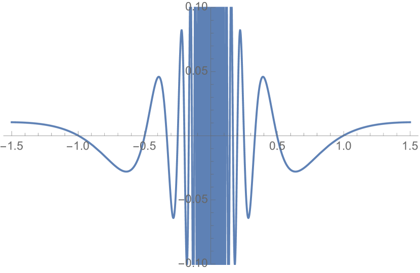
(a) $n$-dependence of $\cosh(\Delta\phi/n)-\cos(\Delta\tau/n)$.

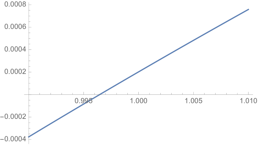
(b) Enlarged plot around $n=1$.

Figure 1: Numerical plots of $\cosh(\Delta\phi/n)-\cos(\Delta\tau/n)$ in eq. (57) with $t=10,l=1,\epsilon=0.1$ .

References

- Parker et al. (2019) D. E. Parker, X. Cao, A. Avdoshkin, T. Scaffidi, and E. Altman, Phys. Rev. X 9, 041017 (2019), arXiv:1812.08657 [cond-mat.stat-mech] .
- Barbón et al. (2019) J. L. F. Barbón, E. Rabinovici, R. Shir, and R. Sinha, JHEP 10, 264, arXiv:1907.05393 [hep-th] .
- Avdoshkin and Dymarsky (2020) A. Avdoshkin and A. Dymarsky, Phys. Rev. Res. 2, 043234 (2020), arXiv:1911.09672 [cond-mat.stat-mech] .
- Dymarsky and Gorsky (2020) A. Dymarsky and A. Gorsky, Phys. Rev. B 102, 085137 (2020), arXiv:1912.12227 [cond-mat.stat-mech] .
- Rabinovici et al. (2021) E. Rabinovici, A. Sánchez-Garrido, R. Shir, and J. Sonner, JHEP 06, 062, arXiv:2009.01862 [hep-th] .
- Cao (2021) X. Cao, J. Phys. A 54, 144001 (2021), arXiv:2012.06544 [cond-mat.stat-mech] .
- Jian et al. (2021) S.-K. Jian, B. Swingle, and Z.-Y. Xian, JHEP 03, 014, arXiv:2008.12274 [hep-th] .
- Kim et al. (2022) J. Kim, J. Murugan, J. Olle, and D. Rosa, Phys. Rev. A 105, L010201 (2022), arXiv:2109.05301 [quant-ph] .
- Rabinovici et al. (2022a) E. Rabinovici, A. Sánchez-Garrido, R. Shir, and J. Sonner, JHEP 03, 211, arXiv:2112.12128 [hep-th] .
- Caputa et al. (2022) P. Caputa, J. M. Magan, and D. Patramanis, Phys. Rev. Res. 4, 013041 (2022), arXiv:2109.03824 [hep-th] .
- Patramanis (2022) D. Patramanis, PTEP 2022, 063A01 (2022), arXiv:2111.03424 [hep-th] .
- Trigueros and Lin (2022) F. B. Trigueros and C.-J. Lin, SciPost Phys. 13, 037 (2022), arXiv:2112.04722 [cond-mat.dis-nn] .
- Hörnedal et al. (2022) N. Hörnedal, N. Carabba, A. S. Matsoukas-Roubeas, and A. del Campo, Commun. Phys. 5, 207 (2022), arXiv:2202.05006 [quant-ph] .
- Fan (2022) Z.-Y. Fan, Phys. Rev. A 105, 062210 (2022), arXiv:2202.07220 [quant-ph] .
- Heveling et al. (2022) R. Heveling, J. Wang, and J. Gemmer, Phys. Rev. E 106, 014152 (2022), arXiv:2203.00533 [cond-mat.stat-mech] .
- Bhattacharjee et al. (2022a) B. Bhattacharjee, X. Cao, P. Nandy, and T. Pathak, JHEP 05, 174, arXiv:2203.03534 [quant-ph] .
- Mück and Yang (2022) W. Mück and Y. Yang, Nucl. Phys. B 984, 115948 (2022), arXiv:2205.12815 [hep-th] .
- Bhattacharya et al. (2022) A. Bhattacharya, P. Nandy, P. P. Nath, and H. Sahu, JHEP 12, 081, arXiv:2207.05347 [quant-ph] .
- Rabinovici et al. (2022b) E. Rabinovici, A. Sánchez-Garrido, R. Shir, and J. Sonner, JHEP 07, 151, arXiv:2207.07701 [hep-th] .
- Liu et al. (2023) C. Liu, H. Tang, and H. Zhai, Phys. Rev. Res. 5, 033085 (2023), arXiv:2207.13603 [cond-mat.str-el] .
- He et al. (2022) S. He, P. H. C. Lau, Z.-Y. Xian, and L. Zhao, JHEP 12, 070, arXiv:2209.14936 [hep-th] .
- Bhattacharjee et al. (2023a) B. Bhattacharjee, P. Nandy, and T. Pathak, JHEP 08, 099, arXiv:2210.02474 [hep-th] .
- Bhattacharjee et al. (2023b) B. Bhattacharjee, X. Cao, P. Nandy, and T. Pathak, JHEP 03, 054, arXiv:2212.06180 [quant-ph] .
- Alishahiha and Banerjee (2023) M. Alishahiha and S. Banerjee, SciPost Phys. 15, 080 (2023), arXiv:2212.10583 [hep-th] .
- Bhattacharjee (2023) B. Bhattacharjee, (2023), arXiv:2302.07228 [quant-ph] .
- Bhattacharya et al. (2023a) A. Bhattacharya, P. Nandy, P. P. Nath, and H. Sahu, JHEP 12, 066, arXiv:2303.04175 [quant-ph] .
- Hashimoto et al. (2023) K. Hashimoto, K. Murata, N. Tanahashi, and R. Watanabe, JHEP 11, 040, arXiv:2305.16669 [hep-th] .
- Patramanis and Sybesma (2023) D. Patramanis and W. Sybesma, (2023), arXiv:2306.03133 [quant-ph] .
- Iizuka and Nishida (2023a) N. Iizuka and M. Nishida, JHEP 11, 065, arXiv:2306.04805 [hep-th] .
- Bhattacharyya et al. (2023) A. Bhattacharyya, D. Ghosh, and P. Nandi, JHEP 12, 112, arXiv:2306.05542 [hep-th] .
- Camargo et al. (2024) H. A. Camargo, V. Jahnke, H.-S. Jeong, K.-Y. Kim, and M. Nishida, Phys. Rev. D 109, 046017 (2024), arXiv:2306.11632 [hep-th] .
- Fan (2023) Z.-Y. Fan, (2023), arXiv:2306.16118 [hep-th] .
- Iizuka and Nishida (2023b) N. Iizuka and M. Nishida, JHEP 11, 096, arXiv:2308.07567 [hep-th] .
- Mohan (2023) V. Mohan, JHEP 11, 222, arXiv:2308.10945 [hep-th] .
- Bhattacharjee et al. (2024) B. Bhattacharjee, P. Nandy, and T. Pathak, JHEP 01, 094, arXiv:2311.00753 [quant-ph] .
- Tang (2023) H. Tang, (2023), arXiv:2312.17416 [hep-th] .
- Bhattacharya et al. (2024) A. Bhattacharya, P. P. Nath, and H. Sahu, (2024), arXiv:2403.03584 [quant-ph] .
- Sasaki (2024) R. Sasaki, (2024), arXiv:2403.06391 [quant-ph] .
- Aguilar-Gutierrez (2024) S. E. Aguilar-Gutierrez, (2024), arXiv:2403.13186 [hep-th] .
- Menzler and Jha (2024) H. G. Menzler and R. Jha, (2024), arXiv:2403.14384 [quant-ph] .
- Carolan et al. (2024) E. Carolan, A. Kiely, S. Campbell, and S. Deffner, (2024), arXiv:2404.03529 [quant-ph] .
- Dymarsky and Smolkin (2021) A. Dymarsky and M. Smolkin, Phys. Rev. D 104, L081702 (2021), arXiv:2104.09514 [hep-th] .
- Magán and Simón (2020) J. M. Magán and J. Simón, JHEP 05, 071, arXiv:2002.03865 [hep-th] .
- Kar et al. (2022) A. Kar, L. Lamprou, M. Rozali, and J. Sully, JHEP 01, 016, arXiv:2106.02046 [hep-th] .
- Caputa and Datta (2021) P. Caputa and S. Datta, JHEP 12, 188, [Erratum: JHEP 09, 113 (2022)], arXiv:2110.10519 [hep-th] .
- Banerjee et al. (2022) A. Banerjee, A. Bhattacharyya, P. Drashni, and S. Pawar, Phys. Rev. D 106, 126022 (2022), arXiv:2205.15338 [hep-th] .
- Avdoshkin et al. (2022) A. Avdoshkin, A. Dymarsky, and M. Smolkin, (2022), arXiv:2212.14429 [hep-th] .
- Camargo et al. (2023) H. A. Camargo, V. Jahnke, K.-Y. Kim, and M. Nishida, JHEP 05, 226, arXiv:2212.14702 [hep-th] .
- Kundu et al. (2023) A. Kundu, V. Malvimat, and R. Sinha, JHEP 09, 011, arXiv:2303.03426 [hep-th] .
- Vasli et al. (2024) M. J. Vasli, K. Babaei Velni, M. R. Mohammadi Mozaffar, A. Mollabashi, and M. Alishahiha, Eur. Phys. J. C 84, 235 (2024), arXiv:2307.08307 [hep-th] .
- Anegawa et al. (2024) T. Anegawa, N. Iizuka, and M. Nishida, (2024), arXiv:2401.04383 [hep-th] .
- Li and Liu (2024) T. Li and L.-H. Liu, (2024), arXiv:2401.09307 [hep-th] .
- Malvimat et al. (2024) V. Malvimat, S. Porey, and B. Roy, (2024), arXiv:2402.15835 [hep-th] .
- Maldacena (2003) J. M. Maldacena, JHEP 04, 021, arXiv:hep-th/0106112 .
- Balasubramanian et al. (2022) V. Balasubramanian, P. Caputa, J. M. Magan, and Q. Wu, Phys. Rev. D 106, 046007 (2022), arXiv:2202.06957 [hep-th] .
- Caputa and Liu (2022) P. Caputa and S. Liu, Phys. Rev. B 106, 195125 (2022), arXiv:2205.05688 [hep-th] .
- Bhattacharjee et al. (2022b) B. Bhattacharjee, S. Sur, and P. Nandy, Phys. Rev. B 106, 205150 (2022b), arXiv:2208.05503 [quant-ph] .
- Caputa et al. (2023a) P. Caputa, N. Gupta, S. S. Haque, S. Liu, J. Murugan, and H. J. R. Van Zyl, JHEP 01, 120, arXiv:2208.06311 [hep-th] .
- Balasubramanian et al. (2023a) V. Balasubramanian, J. M. Magan, and Q. Wu, Phys. Rev. D 107, 126001 (2023a), arXiv:2208.08452 [hep-th] .
- Afrasiar et al. (2023) M. Afrasiar, J. Kumar Basak, B. Dey, K. Pal, and K. Pal, J. Stat. Mech. 2310, 103101 (2023), arXiv:2208.10520 [hep-th] .
- Chattopadhyay et al. (2023) A. Chattopadhyay, A. Mitra, and H. J. R. van Zyl, Phys. Rev. D 108, 025013 (2023), arXiv:2302.10489 [hep-th] .
- Erdmenger et al. (2023) J. Erdmenger, S.-K. Jian, and Z.-Y. Xian, JHEP 08, 176, arXiv:2303.12151 [hep-th] .
- Pal et al. (2023) K. Pal, K. Pal, A. Gill, and T. Sarkar, Phys. Rev. B 108, 104311 (2023), arXiv:2304.09636 [quant-ph] .
- Rabinovici et al. (2023) E. Rabinovici, A. Sánchez-Garrido, R. Shir, and J. Sonner, JHEP 08, 213, arXiv:2305.04355 [hep-th] .
- Nandy et al. (2024) S. Nandy, B. Mukherjee, A. Bhattacharyya, and A. Banerjee, J. Phys. Condens. Matter 36, 155601 (2024), arXiv:2305.13322 [quant-ph] .
- Gautam et al. (2024) M. Gautam, K. Pal, K. Pal, A. Gill, N. Jaiswal, and T. Sarkar, Phys. Rev. B 109, 014312 (2024), arXiv:2308.00636 [quant-ph] .
- Balasubramanian et al. (2023b) V. Balasubramanian, J. M. Magan, and Q. Wu, (2023b), arXiv:2312.03848 [hep-th] .
- Bhattacharya et al. (2023b) A. Bhattacharya, R. N. Das, B. Dey, and J. Erdmenger, (2023b), arXiv:2312.11635 [hep-th] .
- Huh et al. (2023) K.-B. Huh, H.-S. Jeong, and J. F. Pedraza, (2023), arXiv:2312.12593 [hep-th] .
- Beetar et al. (2023) C. Beetar, N. Gupta, S. S. Haque, J. Murugan, and H. J. R. Van Zyl, (2023), arXiv:2312.15790 [hep-th] .
- Mück (2024) W. Mück, (2024), arXiv:2403.05241 [hep-th] .
- Zhou and Chen (2024) B. Zhou and S. Chen, (2024), arXiv:2403.15154 [cond-mat.quant-gas] .
- Caputa et al. (2023b) P. Caputa, J. M. Magan, D. Patramanis, and E. Tonni, (2023b), arXiv:2306.14732 [hep-th] .
- Caputa et al. (2024) P. Caputa, H.-S. Jeong, S. Liu, J. F. Pedraza, and L.-C. Qu, (2024), arXiv:2402.09522 [hep-th] .
- Viswanath and Müller (1994) V. S. Viswanath and G. Müller, The Recursion Method: Application to Many-Body Dynamics (Springer Berlin, Heidelberg, Germany, 1994).
- Nozaki et al. (2014) M. Nozaki, T. Numasawa, and T. Takayanagi, Phys. Rev. Lett. 112, 111602 (2014), arXiv:1401.0539 [hep-th] .
- Caputa et al. (2014) P. Caputa, M. Nozaki, and T. Takayanagi, PTEP 2014, 093B06 (2014), arXiv:1405.5946 [hep-th] .
- He et al. (2014) S. He, T. Numasawa, T. Takayanagi, and K. Watanabe, Phys. Rev. D 90, 041701 (2014), arXiv:1403.0702 [hep-th] .
- Nozaki (2014) M. Nozaki, JHEP 10, 147, arXiv:1405.5875 [hep-th] .
- Asplund et al. (2015) C. T. Asplund, A. Bernamonti, F. Galli, and T. Hartman, JHEP 02, 171, arXiv:1410.1392 [hep-th] .
- Caputa et al. (2015a) P. Caputa, J. Simón, A. Štikonas, and T. Takayanagi, JHEP 01, 102, arXiv:1410.2287 [hep-th] .
- Guo and He (2015) W.-Z. Guo and S. He, JHEP 04, 099, arXiv:1501.00757 [hep-th] .
- Caputa et al. (2015b) P. Caputa, J. Simón, A. Štikonas, T. Takayanagi, and K. Watanabe, JHEP 08, 011, arXiv:1503.08161 [hep-th] .
- Chen et al. (2015) B. Chen, W.-Z. Guo, S. He, and J.-q. Wu, JHEP 10, 173, arXiv:1507.01157 [hep-th] .
- Numasawa (2016) T. Numasawa, JHEP 12, 061, arXiv:1610.06181 [hep-th] .
- Caputa et al. (2017) P. Caputa, Y. Kusuki, T. Takayanagi, and K. Watanabe, J. Phys. A 50, 244001 (2017), arXiv:1701.03110 [hep-th] .
- Guo et al. (2018) W.-Z. Guo, S. He, and Z.-X. Luo, JHEP 05, 154, arXiv:1802.08815 [hep-th] .
- Kusuki and Miyaji (2019) Y. Kusuki and M. Miyaji, JHEP 08, 063, arXiv:1905.02191 [hep-th] .
- Caputa et al. (2019) P. Caputa, T. Numasawa, T. Shimaji, T. Takayanagi, and Z. Wei, JHEP 09, 018, arXiv:1905.08265 [hep-th] .
- Kusuki and Miyaji (2020) Y. Kusuki and M. Miyaji, Phys. Rev. Lett. 124, 061601 (2020), arXiv:1908.03351 [hep-th] .
- Moore and Seiberg (1988) G. W. Moore and N. Seiberg, Phys. Lett. B 212, 451 (1988).
- Verlinde (1988) E. P. Verlinde, Nucl. Phys. B 300, 360 (1988).
- Moore and Seiberg (1989) G. W. Moore and N. Seiberg, Nucl. Phys. B 313, 16 (1989).