Spin-lattice relaxation with non-linear couplings: Comparison between Fermi’s golden rule and extended dissipaton equation of motion

Abstract

Fermi’s golden rule (FGR) offers an empirical framework for understanding the dynamics of spin-lattice relaxation in magnetic molecules, encompassing mechanisms like direct (one-phonon) and Raman (two-phonon) processes. These principles effectively model experimental longitudinal relaxation rates, denoted as $T_{1}^{-1}$. However, under scenarios of increased coupling strength and nonlinear spin-lattice interactions, FGR’s applicability may diminish. This paper numerically evaluates the exact spin-lattice relaxation rate kernels, employing the extended dissipaton equation of motion (DEOM) formalism. Our calculations reveal that when quadratic spin-lattice coupling is considered, the rate kernels exhibit a free induction decay-like feature, and the damping rates depend on the interaction strength. We observe that the temperature dependence predicted by FGR significantly deviates from the exact results since FGR ignores the non-Markovian nature of spin-lattice relaxation. Our methods can be readily applied to other systems with nonlinear spin-lattice interactions and provide valuable insights into the temperature dependence of $T_{1}$ in molecular qubits.

I Introduction

Quantum information technologies, such as quantum computation and quantum sensing, [1, 2] rely on the efficient implementation of qubits. [3, 4] Among various implementations, including superconducting Josephson junctions, [5] photons,[6] and semiconducting quantum dots, [7] paramagnetic coordination complexes stand out due to their inherent synthetic versatility. [8, 9] These molecules possess unpaired electrons, leading to quantized spin states under an applied magnetic field, known as the Zeeman effect. Moreover, metal-organic frameworks (MOFs) and other materials have been utilized to assemble or polymerize these molecules into periodic arrays, enabling chemists to meticulously tune the topology and inter-qubit distance. [10, 11, 12] These techniques provide a systematic way to optimize qubit scalability and performance through chemical design. [3, 4, 13, 14]

In addition to chemical flexibility, molecular qubits offer long coherence times at high temperatures, essential for quantum error correction and fault-tolerant quantum computation. [13, 14] Specifically, the ability of a qubit to execute operations is constrained by its coherence times, determined by both spin phase coherence ($T_{2}$) and longitudinal relaxation ($T_{1}$) times. [15, 13] In applications at low temperatures, $T_{1}$ times notably surpass $T_{2}$, thus exerting minimal influence on qubit performance. [15] However, as temperature rises, $T_{1}$ becomes the primary factor limiting qubit performance. [13] Therefore, a comprehensive understanding of the temperature dependence of $T_{1}$ is crucial for designing qubits suitable for operation under high temperatures.

The key physics behind the $T_{1}$ relaxation time and its temperature dependency are the spin-lattice interactions, i.e., the coupling between the spin system with molecular phonon modes. To understand the relaxation dynamics, the simplest and most widely used models are based on Fermi’s golden rule (FGR). These models are often used to fit the temperature dependence of $T_{1}$ to empirical “processes”, such as the direct (one-phonon) process and Raman (two-phonon) process. [16] However, these empirical models are based on the assumption of weak coupling and Markovian bath, and thus are not always valid. Although there have been exact simulations, such as the hierarchical equations of motion (HEOM) approach, [17, 18] and generalized master equations which take into account non-Markovian baths;[19, 20] these methods all focus on linear spin-lattice interactions, neglecting non-linear couplings. [21] As a result, there is a lack of studies to explore the effects of non-linear spin-lattice interactions and stronger coupling strengths on the temperature dependence of $T_{1}$.

In this study, we address this gap by comparing the FGR predictions with the numerically exact results from the extended dissipaton equation of motion (DEOM) formalism. [22, 21] We demonstrate that the temperature dependence of $T_{1}$ can significantly deviate from the FGR predictions when quadratic spin-lattice interactions are considered. Our results suggest that the temperature dependence of $T_{1}$ is sensitive to the interaction strength and the non-Markovian nature of the spin-lattice relaxation. Our findings provide valuable insights into the temperature dependence of $T_{1}$ in molecular qubits, and can be readily applied to other systems with non-linear spin-lattice interactions.

The rest of the paper is organized as follows. In Sec. II, we introduce the spin-boson model for spin-lattice relaxation, Fermi’s golden rule, and the extended DEOM formalism. In Sec. III, we present the results of our simulations and compare the FGR predictions with the numerically exact results. Finally, in Sec. IV, we conclude our study and discuss the implications of our findings.

II Theory

II.1 Spin-boson model for spin-lattice relaxation

Consider a spin-$\frac{1}{2}$ system interacting with the lattice vibrational modes. The total Hamiltonian reads [23, 24, 25] (We set $\hbar$ as unit.)

$$H_{\text{T}} =\frac{\Delta}{2}\hat{\sigma}_{z}+\frac{1}{2}\sum_{k}\omega_{k}(\hat{p}_{k}^{2}+\hat{q}_{k}^{2})+H_{1}$$

$$=H_{\text{S}}+H_{\text{B}}+H_{1}$$ (1)

with $\Delta$ being the Zeeman energy induced by the static external field and $\{\sigma_{i}\}_{i=x,y,z}$ the Pauli matrices. We consider the spin-lattice coupling Hamiltonian $H_{1}$,

$$H_{1}=\hat{Q}_{\text{S}}(\alpha_{0}+\alpha_{1}\hat{x}_{\text{B}}+\alpha_{2}\hat{x}_{\text{B}}^{2}+\cdots),$$ (2)

where $\hat{Q}_{\text{S}}$ is the spin–subspace operator and $\hat{x}_{\text{B}}\equiv\sum_{k}c_{k}\hat{q}_{k}$ represents the collective lattice mode. The polynomial coefficients $\{\alpha_{0},\alpha_{1},\alpha_{2},\dots\}$ can be parameterized from ab initio calculations. [24]

The influence of the bath on the system dynamics is characterized by the spectral density function,

$$J(\omega)=\frac{\pi}{2}\sum_{k}c_{k}^{2}\delta(\omega-\omega_{k}),\quad\text{for {\hbox{\omega>0}},}$$ (3)

and $J(-\omega)=-J(\omega)$. The spectral density relates to the bare–bath response function $\chi_{\rm B}(t)\equiv i\langle[\hat{x}_{\rm B}(t),\hat{x}_{\rm B}(0)]\rangle_{\rm B}$ via

$$J(\omega)=\frac{1}{2{\rm i}}\int_{-\infty}^{\infty}\!\!{\rm d}t\,e^{\textup{i}\omega t}\chi_{\rm B}(t).$$ (4)

Here, $\hat{x}_{\text{B}}(t)=e^{\textup{i}H_{\text{B}}t}\hat{x}_{\text{B}}e^{-\textup{i}H_{\text{B}}t}$ and $\expectationvalue{(\cdot)}_{\text{B}}\equiv\frac{\tr_{\text{B}}[(\cdot)e^{-\beta H_{\text{B}}}]}{\tr_{\text{B}}[e^{-\beta H_{\text{B}}}]}$ denotes the thermal averages over the bath with $\beta=1/(k_{\text{B}}T)$. We then have the fluctuation–dissipation theorem, [26]

$$\expectationvalue{\hat{x}_{\text{B}}(t)\hat{x}_{\text{B}}(0)}_{\text{B}}=\frac{1}{\pi}\int_{-\infty}^{\infty}\differential{\omega}\frac{e^{-i\omega t}J(\omega)}{1-e^{-\beta\omega}}.$$ (5)

In this work, we use the TLS Hamiltonian in Eq. II.1 to study a simple yet general relaxation process—an out-of-equilibrium spin one-half particle relaxes to equilibrium through the coupling to lattice vibrations. This thermal relaxation process depends on the system operator $\hat{Q}_{\text{s}}$, collective mode $\hat{x}_{\text{B}}$, and the bath polynomial. When $\hat{Q}_{\text{s}}\propto\sigma_{z}$, the TLS becomes the so-called pure decoherence model [27], representing the decoherence contribution from the coupling to lattice vibrations; while $\hat{Q}_{\text{s}}\propto\sigma_{x}\text{ or }\sigma_{y}$ denotes the spin relaxation contribution. Without loss of generality, we will restrict to the case of $\hat{Q}_{\text{s}}\propto\sigma_{x}$ to describe spin-lattice relaxation.

II.2 Fermi’s golden rule rates

In the following, we calculate the thermally averaged FGR rates for the TLS. The FGR rates for the transition from spin state $i$ to $f$ ($i,f=0,1$) are given by [28]

$$k_{f\leftarrow i}(\beta)=\frac{2\pi}{\hbar}\sum_{a}P_{a}(\beta)\sum_{b}\absolutevalue{W_{f,b\leftarrow i,a}}^{2}\delta(E_{f,b}-E_{i,a}).$$ (6)

Here $i,a$ and $f,b$ denote coupled spin-vibrational states $\ket{i,a}$ and $\ket{f,b}$; $P_{a}(\beta)=\exp(-\beta\omega_{a})/Z$ denotes the Boltzmann weight for the $a$-th vibrational state where $Z=\sum_{a}\exp(-\beta\omega_{a})$ is the bare–bath partition function; and $W_{f,b\leftarrow i,a}=\matrixelement{f,b}{H_{1}}{i,a}$ denotes the transition matrix element. For the FGR calculation, we only consider $\hat{Q}_{\text{s}}=\sigma_{x}$, i.e., the relaxation contribution from the spin-lattice interaction. Thus, only two terms are non-vanishing: $W_{f,1\leftarrow i,0}=\matrixelement{1,b}{z(\hat{x}_{\text{B}})}{0,a}$ and $W_{f,0\leftarrow i,1}=\matrixelement{0,b}{z(\hat{x}_{\text{B}})}{1,a}$.

The discrete Eq. 6 for $k_{f\leftarrow i}(T)$ can be recast in terms of correlation function (see Eq. 27):

$$k_{f\leftarrow i}(\beta)=\int_{-\infty}^{\infty}\differential{t}e^{\pm\textup{i}\epsilon t}\expectationvalue{z(\hat{x}_{\text{B}}(t))z(\hat{x}_{\text{B}}(0))}_{\text{B}},$$ (7)

where we use the upper sign ($+$ in this equation) in the exponential denotes the $1\leftarrow 0$ process, and the lower sign ($-$) denotes the $0\leftarrow 1$ process, respectively. The upper and lower sign convention will be consistently applied henceforth. Here, $\epsilon$ denotes the energy difference between states 0 and 1. In other words, the FGR rates depend on the time correlation functions of polynomial $z(\hat{x}_{\text{B}})$. In moderate coupling strength, we are safe to truncate the polynomial up to the second order that $z(x)=\alpha_{0}+\alpha_{1}x+\alpha_{2}x^{2}$. Additionally, we can also absorb the zero-th order interaction $\alpha_{0}$ into the quantum system $H_{\text{s}}$. When $\alpha_{0}=0$, the spin states $\ket{0}$ and $\ket{1}$ are eigen states, hence $\epsilon=\Delta$. Otherwise we have to calculate $\epsilon$ from diagonalize $H_{s}+\alpha_{0}\sigma_{x}$. With these considerations, the calculations of $T^{-1}$ using FGR becomes straightforward, which are outlined in Appendix A. It is noteworthy that two terms,

$$\alpha_{1}^{2}\expectationvalue{\hat{x}_{\text{B}}(t)\hat{x}_{\text{B}}(0)}_{\text{B}},\text{ and }\alpha_{2}^{2}\expectationvalue{\hat{x}_{\text{B}}^{2}(t)\hat{x}_{\text{B}}^{2}(0)}_{\text{B}},$$

prove to be finite, while the cross linear-quadratic terms in the correlation function vanish. After some algebra, we obtain closed expressions for the FGR relaxation rates given by

$$k_{f\leftarrow i}=\alpha_{1}^{2}k_{f\leftarrow i}^{\text{(1)}}+\alpha_{2}^{2}k_{f\leftarrow i}^{\text{(2)}},$$ (8a)

$$k_{f\leftarrow i}^{\text{(1)}}=2\frac{J(\pm\epsilon)}{1-e^{\mp\beta\epsilon}},$$ (8b)

$$k_{f\leftarrow i}^{\text{(2)}}=\frac{4}{\pi}\int_{-\infty}^{\infty}\differential{\omega}\frac{J(\omega)}{1-e^{-\beta\omega}}\frac{J(\omega\pm\epsilon)}{e^{\beta(\omega\pm\epsilon)}-1},$$ (8c)

with superscript $(1)$ and $(2)$ denoting $\hat{x}_{\text{B}}$ and $\hat{x}_{\text{B}}^{2}$ coupling term [24], respectively.

Notably, in the computation of the FGR rate detailed in Appendix A, the quadratic component of $T_{1}^{-1}$ introduces an oscillatory term expressed in Eq.32. However, within the FGR regime, this term cannot converge to a finite value and thus is not included in the final rate calculation. Intriguingly, we do observe oscillating behaviors of the rate kernels in the extended DEOM simulations, as discussed in Sec. III.

II.3 The extended DEOM for both linear and quadratic environments

In the standard HEOM formalism, only the linear coupling to the bath mode $\hat{x}_{\text{B}}$ is considered.[21, 18] However, to accurately model the spin-lattice interaction dynamics requires the explicit considerations of non-linear coupling at least to the second order ($\hat{x}_{\text{B}}^{2}$), since the relaxations with two phonon processes are very common in experiments. Fortunately, the extended dissipaton equation of motion (DEOM) formalism, by R.-X. Xu and colleagues, extends the HEOM methods for non-linear interactions up to the quadratic order.[22, 21, 29] This study employs the extended DEOM formalism to investigate the spin-lattice relaxation. Subsequently, we provide a concise introduction to this method.

Similar to the HEOM formalism, the extended DEOM requires to expand the bath correlation function in finite exponential series,

$$\expectationvalue{\hat{x}_{\text{B}}(t)\hat{x}_{\text{B}}(0)}_{\text{B}}=\sum_{k}^{K}\eta_{k}e^{-\gamma_{k}t},$$ (9)

where $K$ sets of parameters $\eta_{k}$ and $\gamma_{k}$ are generally obtained from fitting or spectral function decomposition such as the Padé decomposition. [30, 31] In contrast to the auxiliary density matrix interpretation of HEOM, DEOM employs a quasi-particle interpretation of such decomposition that leads to the following algebra

$$\hat{x}_{\text{B}}=\sum_{k}^{K}\hat{f}_{k},$$ (10)

$$\expectationvalue{\hat{f}_{k}(t)\hat{f}_{k^{\prime}}(0)}_{\text{B}}=\delta_{kk^{\prime}}\eta_{k}e^{-\gamma_{k}t}.$$ (11)

Here, $\{\hat{f}_{k}\}_{k=1}^{K}$ are the so-called dissipaton operators, where the dissipatons are independent quasi-particles that represent the collective bath.

With the dissipaton operators, we can represent the total system dynamics as a set of equations of motion for the dissipaton density operators (DDOs). To begin, we know the composite system density operator $\rho_{\text{T}}$ satisfies the von Neumann equation

$$\dot{\rho}_{\text{T}}(t)=-\textup{i}\commutator{H_{\text{T}}}{\rho_{\text{T}}(t)}.$$ (12)

The DDOs can be defined as

$$\rho_{\bm{n}}^{(n)}(t)=\rho_{n_{1}\dots n_{K}}^{(n)}(t)=\tr_{\text{B}}[(\hat{f}_{K}^{n_{K}}\dots\hat{f}_{1}^{n_{1}})^{\circ}\rho_{\text{T}}(t)].$$ (13)

Here, index $\bm{n}\equiv\{n_{1},\dots,n_{K}\}$ denotes the configuration, and $n=n_{1}+\dots+n_{K}$ denotes the total number of disspaton exitations. The notation $(\cdots)^{\circ}$ denotes the irreducible representation. For bosonic dissipaton, as is in the case of lattice vibration, we have $(\hat{f}_{k}\hat{f}_{k^{\prime}})^{\circ}=(\hat{f}_{k^{\prime}}\hat{f}_{k})^{\circ}$. With these, we can know the reduced system density operator are given by $\rho_{\text{S}}\equiv\rho_{\bm{0}}^{(0)}$. Refs. [22, 21] show that the reduced system dynamics given by Eq. 2 is obtained by applying the dissipaton algebra, including the generalized generalized Wick’s theorems (GWT-I and GWT-II). The equations of motion of $\{\rho_{\bm{n}}^{(n)}\}$ read

$$\dot{\rho}_{\bm{n}}^{(n)} =-(\textup{i}\mathcal{L}_{\text{s}}+\sum_{k}n_{k}\gamma_{k})\rho_{\bm{n}}^{(n)}-\textup{i}(\alpha_{0}+\alpha_{2}\expectationvalue{\hat{x}_{\text{B}}^{2}}_{\text{B}})\mathcal{A}\rho_{\bm{n}}^{(n)}$$ (14)

$$-\textup{i}\alpha_{1}\sum_{k}(\mathcal{A}\rho_{\bm{n}_{k}^{+}}^{(n+1)}+n_{k}\mathcal{C}_{k}\rho_{\bm{n}_{k}^{-}}^{(n-1)})-2\textup{i}\alpha_{2}\sum_{kk^{\prime}}n_{k}\mathcal{C}_{k}\rho_{\bm{n}_{kk^{\prime}}^{+-}}^{(n)}$$

$$-\textup{i}\alpha_{2}\sum_{kk^{\prime}}\left[\mathcal{A}\rho_{\bm{n}_{kk^{\prime}}^{++}}^{(n-2)}+n_{k}(n_{k^{\prime}}-\delta_{kk^{\prime}})\mathcal{B}_{kk^{\prime}}\rho_{\bm{n}_{kk^{\prime}}^{--}}^{(n-2)}\right],$$

with some of the convenient operators used above defined as the following,

$$\mathcal{L}_{\text{s}}\hat{O}\equiv\commutator{H_{\text{s}}}{\hat{O}},$$ (15a)

$$\mathcal{A}\hat{O}\equiv\commutator{\hat{Q}_{\text{s}}}{\hat{O}},$$ (15b)

$$\mathcal{B}_{kk^{\prime}}\hat{O}\equiv\eta_{k}\eta_{k^{\prime}}\hat{Q}_{\text{s}}\hat{O}-\eta_{\bar{k}}^{*}\eta_{\bar{k}^{\prime}}^{*}\hat{O}\hat{Q}_{\text{s}},$$ (15c)

$$\mathcal{C}_{k}\hat{O}\equiv\eta_{k}\hat{Q}_{\text{s}}\hat{O}-\eta_{\bar{k}}^{*}\hat{O}\hat{Q}_{\text{s}}.$$ (15d)

For later use, we introduce a compact notation,

$$\dot{\bm{\rho}}(t)=-\textup{i}\bm{\mathcal{L}}(t)\bm{\rho}(t).$$ (16)

Here, $\bm{\rho}(t)=\{\rho_{\bm{n}}^{(n)};n=0,1,2,\dots\}$ denotes the set of DDOs. The equations of motion encoded in Eq. 14 are represented by the DEOM-space dynamics generator $\bm{\mathcal{L}}(t)$.

II.4 Rate kernel from the extended DEOM formalism

As introduced in Sec. II.3, DDO equations of motions (Eq. 14) provide a numerically exact recipe for the reduced system dynamics. We can go one step further to extract the rate kernels for the spin-lattice relaxation by applications of the projection operator techniques. [32]

Following  ref. [32], we use the Nakajima-Zwanzig projection operator technique onto the DDOs. [33, 34] For the reduced system density $\rho^{(0)}$, it’s intuitive to define $\mathcal{P}$ and $\mathcal{Q}\equiv\mathrm{1}-\mathcal{P}$ as the following

$$\begin{gathered}\mathcal{P}\rho^{(0)}=P_{0}(t)\outerproduct{0}{0}+P_{1}(t)\outerproduct{1}{1},\\ \mathcal{Q}\rho^{(0)}=\rho^{(0)}_{01}(t)\outerproduct{0}{1}+\rho^{(0)}_{10}(t)\outerproduct{1}{0},\end{gathered}$$ (17)

where $\mathcal{P}$ and $\mathcal{Q}$ represents the population and coherence, respectively. The projection definitions can then be generalized to the full DDO-space by

$$\begin{gathered}\bm{\mathcal{P}}\bm{\rho}(t)=\{\mathcal{P}\rho^{0}(t);0,0,\dots\}\equiv\bm{p}(t),\\ \bm{\mathcal{Q}}\bm{\rho}(t)=\{\mathcal{Q}\rho^{0}(t);\rho^{(n>0)}_{\bm{n}}(t)\}\equiv\bm{\sigma}(t),\end{gathered}$$ (18)

such that Eq. 16 can be recasted into:

$$\begin{pmatrix}\dot{\bm{p}}\\ \dot{\bm{\sigma}}\end{pmatrix}=-\textup{i}\begin{pmatrix}\bm{\mathcal{PLP}}&\bm{\mathcal{PLQ}}\\ \bm{\mathcal{QLP}}&\bm{\mathcal{QLQ}}\end{pmatrix}\begin{pmatrix}\bm{p}\\ \bm{\sigma}\end{pmatrix}.$$ (19)

Formally, one can integrate the equation for the $\bm{\mathcal{Q}}$-space density $\bm{\sigma}$ and obtain solution:

$$\bm{\sigma}(t)=e^{-\textup{i}\bm{\mathcal{QL}}t}\bm{\sigma}(0)-\textup{i}\int_{0}^{t}\differential{\tau}e^{-\textup{i}\bm{\mathcal{QL}}(t-\tau)}\bm{\mathcal{QL}}\bm{p}(\tau).$$ (20)

By inserting this formal solution of $\bm{\sigma}(t)$ to the equations of motion for $\bm{\mathcal{P}}$-space density $\bm{p}$, one obtains:

$$\begin{gathered}\dot{\bm{p}}(t)=-\textup{i}\bm{\mathcal{PL}}e^{-\textup{i}\bm{\mathcal{QL}}t}\bm{\sigma}(0)+\int_{0}^{t}\differential{\tau}\bm{\mathcal{K}}(t-\tau)\bm{p}(\tau),\\ \bm{\mathcal{K}}(t)=-\bm{\mathcal{PL}}e^{-i\bm{\mathcal{QL}}t}\bm{\mathcal{QLP}}.\end{gathered}$$ (21)

In practice, the standard factorization $\bm{\rho}(0)=\rho_{\text{S}}(0)\otimes\rho_{\text{B}}^{\text{eq}}$ of the initial condition is used, meaning $\rho^{(n>0)}_{\bm{n}}(t)=0$. As a result, projected system density $\bm{p}(t)$ satisfies intergo-differential equation

$$\dot{\bm{p}}(t)=\int_{0}^{t}\differential{\tau}\bm{\mathcal{K}}(t-\tau)\bm{p}(\tau).$$ (22)

The rate kernel $\bm{\mathcal{K}}(t)$ encodes the full non-Markovian dynamics of the reduced system, and we can readily extract the $T_{1}^{-1}$ rate from $\bm{\mathcal{K}}(t)$ . In particular, the reduced population of spin state $a$ ($a=0,1$) satisfies the following kinetic equation:

$$\dot{P}_{a}(t)=- \int_{0}^{t}\differential{\tau}\mathcal{K}_{b\leftarrow a}(t-\tau)P_{a}(\tau)+$$ (23)

$$\int_{0}^{t}\differential{\tau}\mathcal{K}_{a\leftarrow b}(t-\tau)P_{b}(\tau).$$

In the Markovian limit, the above kinetic equation becomes simpler: $\dot{P}_{1}(t)=k_{0\leftarrow 1}P_{1}(t)+k_{1\leftarrow 0}P_{0}(t)$, where

$$k_{a\leftarrow b}=\int_{0}^{\infty}\differential{\tau}\mathcal{K}_{a\leftarrow b}(\tau),\quad a,b\in\{0,1\}.$$ (24)

Here, $k_{0\leftarrow 1}$ and $k_{1\leftarrow 0}$ encode the long time behaviour of the rate kernel components $\mathcal{K}_{0\leftarrow 1}$ and $\mathcal{K}_{1\leftarrow 0}$. In the context of spin-lattice relaxation,

$$T_{1}^{-1}=k_{0\leftarrow 1}+k_{1\leftarrow 0}.$$ (25)

III Results and Discussions

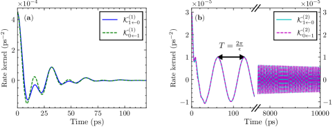
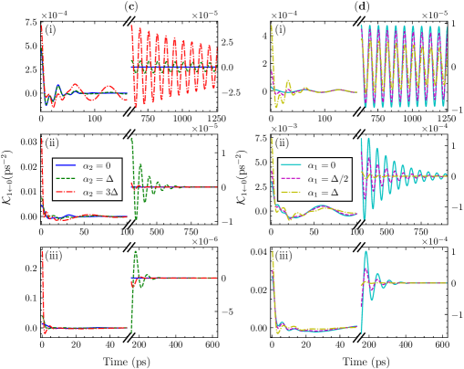
Figure 1: Characteristic rate kernels illustrating $\hat{x}_{\text{B}}$-, $\hat{x}_{\text{B}}^{2}$-, and $\alpha_{1}\hat{x}_{\text{B}}+\alpha_{2}\hat{x}_{\text{B}}^{2}$ spin-lattice interactions. Panel (a) displays the kernel with exclusive $\hat{x}_{\text{B}}$-coupling ($\alpha_{1}=10/3\,\textup{cm}^{-1}$, $\alpha_{2}=0\,\textup{cm}^{-1}$). Panel (b) illustrates the scenario of exclusive $\hat{x}_{\text{B}}^{2}$-coupling ($\alpha_{1}=0\,\textup{cm}^{-1}$, $\alpha_{2}=10/3\,\textup{cm}^{-1}$). Notably, both $\mathcal{K}_{1\leftarrow 0}^{(2)}$ and $\mathcal{K}_{0\leftarrow 1}^{(2)}$ initiate free induction decay like profile with a frequency $\epsilon=\Delta$ after initial dynamics. In panels (a) and (b), $\lambda=0.001$. Panel (c) portrays the impact of $\alpha_{2}$ on $\mathcal{K}^{(1)}$ while keeping $\alpha_{1}=1$. Panel (d) illustrates the influence of $\alpha_{1}$ on $\mathcal{K}^{(2)}$ with $\alpha_{2}=1$. In panels (c) and (d), sub-panels (i-iii) correspond to $\lambda=0.001,0.01,0.03$, respectively. Only the $0\to 1$ rate is plotted for clarity. The following parameters are consistent across all four panels: $\alpha_{0}=0\,\textup{cm}^{-1}$, $\Delta=\zeta=10/3\,\textup{cm}^{-1}$, $\omega_{\text{B}}=10\,\textup{cm}^{-1}$, and temperature $T=53.2\,\mathrm{K}$.

In the following, we calculate the rate kernel for the spin-lattice relaxation dynamics using the extended DEOM formalism described in Sec. II.3 and II.4. Here we consider then rate kernel of solely linear (denoted as $\mathcal{K}^{(1)}$), solely quadratic ($\mathcal{K}^{(2)}$) and general mixed linear-quadratic ($\mathcal{K}$) system-bath coupling, respectively. With the rate kernel results, we evaluate the Markovian limit of the $T_{1}^{-1}$ rates given by Eq. 25, and make a comparison with the FGR rates given by Eqs 8.

We focus on the spin-relaxation through a local lattice vibrational mode with a characteristic frequency of $\omega_{\text{B}}$, meanwhile this characteristic mode couples to all the other lattice vibrations, i.e., the bath modes. This type of system-oscillator-bath is widely applied to study dissipative dynamics, [25, 35, 36] and can be readily mapped to the simple spin-boson model (Eq. II.1) via the well-established canonical transformation [37, 35]. To this end, the local mode relaxation scheme can be described by a Brownian motion spectral function [22] given by

$$J(\omega)=\imaginary\frac{2\lambda\omega_{B}^{2}}{\omega_{B}^{2}-\omega^{2}-i\omega\zeta}.$$ (26)

Here, $\lambda$ denotes the interaction strength, and we assume the friction function $\zeta(\omega)=\zeta$ is frequency independent [36, 29]. With expression Eq. 26 for $J(\omega)$, we construct the extended DEOM by decomposing correlation function Eq. 5 into a few dissipatons using the time-domain Prony fitting method. [31]

III.1 Rate kernels of linear and quadratic coupling

In FIG. 1, we present characteristic rate kernels for the spin-lattice relaxation dynamics. Specifically, we consider a spin with Zeeman energy $\Delta=10/3\,\textup{cm}^{-1}$, of the characteristic energy of W-band ($100\mathrm{GHz}$) Electron Paramagnetic Resonance (EPR) experiment. This spin couples to a characteristic local phonon mode centered at frequency $\omega_{\text{B}}=10\,\textup{cm}^{-1}$.

Notably, the behaviors of the rate kernel as a function of time are drastically different for $\hat{x}_{\text{B}}$- and $\hat{x}_{\text{B}}^{2}$- spin-lattice coupling. The linear kernel $\mathcal{K}^{(1)}$ completely decays (FIG. 1 (a)) within a few picoseconds, which is the typical time it takes for lattice phonon oscillation. In contrast, the quadratic kernels $\mathcal{K}^{(2)}$ continue to oscillate without much decay (FIG. 1 (b)), when the coupling is weak. Moreover, the long time limit of the $\mathcal{K}^{(2)}$ kernels exhibits a free induction decay (FID) like feature, with a frequency $\epsilon=\Delta$, despite the initial dynamics have a more complicated structure.

As we indicated in Sec. II.2, the FGR rates for the $\hat{x}_{\text{B}}^{2}$ coupling indeed contain an oscillating term (Eq. 32), which agrees with the FID-like feature of the $\mathcal{K}^{(2)}$ kernels calculated from extended HEOM. However, the FGR calculations do not capture the decay of the oscillating term, so the oscillating terms cannot convert to a finite value and are thus not included in the final rate calculation. This indicates simple perturbation theories ignore some contributions to the rates. In particular, these ignored interactions can somehow damp the oscillating integral Eq. 32 term. To understand the effect of the neglected contribution, we propose a simple model in Appendix. B. The simple model demonstrates when the decay rate, denoted $\Gamma$, is comparable with the oscillation frequency, the neglected contribution can significantly alter the relaxation rate.

The extended DEOM simulations reveal that the decay rate $\Gamma$ of the FID-like kernel $\mathcal{K}^{(2)}$ depends on the coupling strength $\lambda$, and can be notably enhanced when the quadratic coupling is mixed with linear coupling. As illustrated in FIG. 1 (c.i-iii), the decay rate $\Gamma$ increases with the coupling strength. In addition, panel (d) demonstrates when linear coupling is added to quadratic coupling, the decay rate $\Gamma$ is significantly enhanced when compared with the purely $\hat{x}_{\text{B}}^{2}$-coupling (panel (b)). Notably, the decay is greatly enhanced even for weak coupling ($\lambda=0.001$). Overall, these comparisons indicate the FGR rates ignores 1) all the higher-order terms in the perturbation series, and 2) the interaction between the linear and quadratic coupling term. On the other hand, the numerical exact DEOM simulations capture the higher order terms in the perturbation series and the interaction between the linear and quadratic coupling term (Eq. 14).

Overall, we demonstrate a stronger coupling and a mixed linear quadratic interaction can enhance the relaxation rate of the FID-like rate kernel. As we soon demonstrate in Section III.2, this subtlety becomes a source of contribution that leads to the failure of FGR rate estimations, which can qualitatively alter the temperature dependence of $T_{1}^{-1}$.

III.2 The temperature dependency of $T^{-1}$ rate

With rate kernels readily obtained by the extended DEOM formalism, we are in the position to evaluate the $T_{1}^{-1}$ rate using Eq. 25. In particular, we focus on how $T_{1}^{-1}$ depends on temperature.

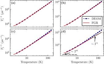
Figure 2: $T_{1}^{-1}$ as a function of temperature in solely $\hat{x}_{\text{B}}$-coupling. Panels (a-d) correspond to interaction strength $\lambda=0.001,0.003,0.01,0.03$, respectively. The following parameters are used: $\alpha_{1}=10/3\,\textup{cm}^{-1}$, $\alpha_{0}=\alpha_{2}=0\,\textup{cm}^{-1}$, $\Delta=\zeta=10/3\,\textup{cm}^{-1}$, $\omega_{\text{B}}=10\,\textup{cm}^{-1}$.

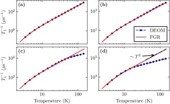
Figure 3: $T_{1}^{-1}$ as a function of temperature in solely $\hat{x}_{\text{B}}^{2}$-coupling. Panels (a-d) correspond to interaction strength $\lambda=0.001,0.003,0.01,0.03$, respectively. The following parameters are used: $\alpha_{2}=10/3\,\textup{cm}^{-1}$, $\alpha_{0}=\alpha_{1}=0\,\textup{cm}^{-1}$, $\Delta=\zeta=10/3\,\textup{cm}^{-1}$, $\omega_{\text{B}}=10\,\textup{cm}^{-1}$.

FIGs. 2 and 3 compare $T_{1}^{-1}$ predicted by the FGR and DEOM for the solely linear and solely quadratic coupling case, respectively. Notably, the FGR results agree with that of DEOM in the weak coupling limits across a wide range of temperatures in both cases, despite the quadratic dynamics clearly show long term memories (FIG. 1). Such agreement indicates when the interaction strength $\lambda$ is small, the higher order terms in the perturbation series, and the damping of the oscillating rate terms are not important. Consequently, in the weak coupling limit, the temperature scaling of $T_{1}^{-1}$ for linear and quadratic coupling are $T$ and $T^{2}$, respectively, to which both the FGR and DEOM results agree.

Nevertheless, FGR rates indeed deviate from DEOM when stronger coupling is present. In particular, panel (c) and (d) of FIGs. 2 and 3 indicate FGR tend to underestimate the $T_{1}^{-1}$ in linear coupling, and overestimate the $T_{1}^{-1}$. These panels demonstrate the well known high temperature scaling laws fails when the coupling is strong. Overall, the quadratic rates tend to have stronger deviations than the linear rates.

Finally, we demonstrate that more dramatic deviations can occur when we consider the case of a mixed linear quadratic spin-lattice relaxation channel. In particular, FIG. 4 demonstrates the FGR overestimates both the values and scaling of $T_{1}^{-1}$ at high-temperature regime, when we add some quadratic coupling when $\alpha_{1}$ is fixed. In comparison, when $\alpha_{2}$ is fixed and some linear character is added to the spin-lattice interaction, we observe a lesser degree of deviation. (FIG. 5)

Overall, we demonstrate when the spin-lattice coupling is strong, we cannot simply treat the dynamics and rates with perturbation theory. In addition, although the linear and quadratic coupling are generally treated as independent in literature, [24] we demonstrate the interactions are very important for the $T_{1}^{-1}$ rates when the coupling is somewhat stronger.

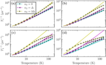
Figure 4: The effect of $\alpha_{2}$ on $T_{1}^{-1}$ as a function of temperature when $\alpha_{1}=10/3\,\textup{cm}^{-1}$ is fixed. Panels (a-d) correspond to interaction strength $\lambda=0.001,0.003,0.01,0.03$, respectively. Other parameters are: $\alpha_{0}=0\,\textup{cm}^{-1}$, $\Delta=\zeta=10/3\,\textup{cm}^{-1}$, $\omega_{\text{B}}=10\,\textup{cm}^{-1}$.

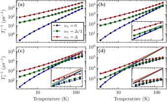
Figure 5: The effect of $\alpha_{1}$ on $T_{1}^{-1}$ as a function of temperature when $\alpha_{2}=10/3\,\textup{cm}^{-1}$ is fixed. Panels (a-d) correspond to interaction strength $\lambda=0.001,0.003,0.01,0.03$, respectively. Other parameters are: $\alpha_{0}=0\,\textup{cm}^{-1}$, $\Delta=\zeta=10/3\,\textup{cm}^{-1}$,$\omega_{\text{B}}=10\,\textup{cm}^{-1}$.

IV Conclusion

In this work, we apply the extend DEOM method to examine the validity of FGR in modeling the dynamics of spin-lattice interaction. The numerical exact DEOM approach reveals the free induction decay (FID) feature of quadratic coupling dynamics. The decay rate of the kernel can be very slow, indicating strong non-Markovian nature for the two-phonon processes encoded in $\hat{x}_{\text{B}}^{2}$-coupling. We demonstrate this damping rate depends on 1) the coupling strength, and 2) the interactions between the one and two phonon processes. Indeed, damping of the rate kernel is completely neglected in perturbation treatments as they are encoded in higer order interactions. Consequently, methods such as FGR and Markovian master equations fail to correctly predict the relaxation dynamics and the temperatures dependencies when the coupling is strong.

Looking forward, these findings as well as the methods presented in this work should be very useful in understand qubits relaxation dynamics in the field of quantum information. One particular applications of this technique can be used to study spin-lattice relaxation of the NV center,[38] which is a three level system that can encode more complicated and interesting dynamics. In addition, the method here can be coupling with data driven methods such as DMD,[39] provide the possibility of studying spin-relaxation dynamics for systems of large dimension. These works are on-going.

Appendix A Fermi’s golden rule calculation of $T_{1}$

The discrete FGR rate (Eq. 6) is recast into integration of continuous correlation function:

$$k_{f\leftarrow i}(\beta) =\int_{-\infty}^{\infty}\differential{t}\sum_{a,b}\frac{e^{-\beta\omega_{a}}}{Z}\matrixelement{a}{z(\hat{x}_{\text{B}})}{b}\matrixelement{b}{z(\hat{x}_{\text{B}})}{a}e^{\textup{i}(E_{b}-E_{a}\mp\epsilon)t},$$ (27)

$$=\int_{-\infty}^{\infty}\differential{t}\frac{e^{\pm\textup{i}\epsilon t}}{Z}\sum_{a}\matrixelement{a}{e^{\textup{i}H_{\text{B}}t}z(\hat{x}_{\text{B}})e^{-\textup{i}H_{\text{B}}t}z(\hat{x}_{\text{B}})e^{-\beta H_{\text{B}}}}{a},$$ (28)

$$=\int_{-\infty}^{\infty}\differential{t}e^{\pm\textup{i}\epsilon t}\expectationvalue{z(\hat{x}_{\text{B}}(t))z(\hat{x}_{\text{B}}(0)}_{\text{B}}.$$ (29)

where $\pm$ signs denote the $1\leftarrow 0$ and $0\leftarrow 1$ process, respectively. Here, $\epsilon$ denotes energy difference between state 0 and 1. When $\alpha_{0}=0$, $\epsilon=\Delta$. Otherwise we diagonalize $H_{\text{s'}}=\frac{\Delta}{2}\sigma_{z}+\alpha_{0}\sigma_{x}$ to obtain $\epsilon$.

In this work, we truncate polynomial to $z(x)=\alpha_{1}x+\alpha_{2}x^{2}$. We now show that many terms in the correlation function vanish. Particularly, terms with odd number of bath operators vanish, e.g., three operator terms like $\expectationvalue{\hat{x}_{\text{B}}^{2}(t)\hat{x}_{\text{B}}(0)}_{\text{B}}$. This is because when taking thermal averages of non-interacting boson operators, three term creation/annihilation operators averages vanish. To demonstrate this, we suppose $\hat{x}_{\text{B}}\equiv\sum_{k}c_{k}\hat{q}_{k}$ and $\hat{q}_{k}=\frac{1}{\sqrt{2}}(\hat{b}^{\dagger}_{k}+\hat{b}_{k})$. For example, correlation function $\expectationvalue{\hat{x}_{\text{B}}^{2}(t)\hat{x}_{\text{B}}(0)}_{\text{B}}$ will consist of three operator term such as

$$\expectationvalue{\hat{b}_{j}\hat{b}_{k}\hat{b}_{l}^{\dagger}}_{\text{B}}\propto\Tr[\hat{b}_{j}\hat{b}_{k}\hat{b}_{l}^{\dagger}e^{-\beta H_{\text{B}}}].$$

Using identities $\hat{b}_{l}^{\dagger}e^{-\beta H_{\text{B}}}=e^{-\beta H_{\text{B}}}e^{\beta H_{\text{B}}}\hat{b}_{l}^{\dagger}e^{-\beta H_{\text{B}}}=e^{\beta\omega_{l}}e^{-\beta H_{\text{B}}}\hat{b}_{l}^{\dagger}$, cyclic property of trace and commutation relations, we can can show these three-operator averages indeed vanishes. Hence, $k_{f\leftarrow i}$ has only two contributions — $\alpha_{1}^{2}\expectationvalue{\hat{x}_{\text{B}}(t)\hat{x}_{\text{B}}(0)}_{\text{B}}$, and $\alpha_{2}^{2}\expectationvalue{\hat{x}_{\text{B}}^{2}(t)\hat{x}_{\text{B}}^{2}(0)}_{\text{B}}$, which we refer to as the linear term ($k_{f\leftarrow i}^{(1)}$) and quadratic term ($k_{f\leftarrow i}^{(2)}$), respectively.

To calculate $k_{f\leftarrow i}^{(1)}$, we just substitute Eq. 5 into Eq. 7 and obtain

$$k_{f\leftarrow i}^{(1)}(\beta)=2\int_{-\infty}^{\infty}\differential{\omega}\frac{J(\omega)}{1-e^{-\beta\omega}}\delta(\omega\pm\epsilon).$$ (30)

Using the fact $J(\omega)$ is an odd function, we conclude the linear term contribution to $T_{1}^{-1}$ is $k_{1\leftarrow 0}^{(1)}+k_{0\leftarrow 1}^{(1)}=2J(\epsilon)\coth{(\frac{\beta\epsilon}{2})}$. It is easy to verify detailed balance $k_{0\leftarrow 1}=e^{-\beta\epsilon}k_{1\leftarrow 0}$ is satisfied for the FGR rates. Notably, we observe the temperature scaling of $k^{(0)}_{f\leftarrow i}$ does not depend on the spectral density: In the high temperature limit ($\beta\epsilon\ll 1$), $T_{1}^{-1}\propto T^{-1}$; In the low temperature limit ($\beta\to\infty$), $T_{1}^{-1}$ become temperature independent that $T_{1}^{-1}\propto T^{0}$.

To calculate $k_{f\leftarrow i}^{(2)}$, we need first evaluate $\expectationvalue{\hat{x}_{\text{B}}^{2}(t)\hat{x}_{\text{B}}^{2}(0)}_{\text{B}}$. Specifically, using $\hat{x}_{\text{B}}(t)=\sum_{j}\frac{c_{j}}{\sqrt{2}}(\hat{b}_{j}^{\dagger}e^{\textup{i}\omega_{j}t}+\hat{b}_{j}e^{-\textup{i}\omega_{j}t})$, definition of the spectral function (Eq. 3), the fact that $J(\omega)$ is a odd function, and Wick’s theorem, we obtain

$$\expectationvalue{\hat{x}_{\text{B}}^{2}(t)\hat{x}_{\text{B}}^{2}(0)}_{\text{B}}= 2\int_{0}^{\infty}\frac{\differential{\omega}}{\pi}\frac{J(\omega)}{e^{\beta\omega}-1}\int_{-\infty}^{\infty}\frac{\differential{\omega^{\prime}}}{\pi}\frac{J(\omega^{\prime})}{1-e^{-\beta\omega^{\prime}}}\exp[\textup{i}(\omega-\omega^{\prime})t]+$$ (31)

$$2\int_{0}^{\infty}\frac{\differential{\omega}}{\pi}\frac{J(\omega)}{1-e^{-\beta\omega}}\int_{-\infty}^{\infty}\frac{\differential{\omega^{\prime}}}{\pi}\frac{J(\omega^{\prime})}{e^{\beta\omega^{\prime}}-1}\exp[-\textup{i}(\omega-\omega^{\prime})t]+$$

$$\left[\int_{0}^{\infty}\frac{\differential{\omega}}{\pi}J(\omega)\coth{\frac{\beta\omega}{2}}\right]^{2}.$$

Substitute this result into Eq. 7, we observe time integration $e^{\pm\textup{i}\epsilon t}$, along with complex phases in the first two terms, yields delta functions. After frequency integration, this results in a finite rate value. However, the last term in the correlation function contributes an oscillating integral that does not converge to a finite value:

$$\left[\int_{0}^{\infty}\frac{\differential{\omega}}{\pi}J(\omega)\coth{\frac{\beta\omega}{2}}\right]^{2}\int_{-\infty}^{\infty}\differential{t}e^{\pm\textup{i}\epsilon t}$$ (32)

Notably, both $0\to 1$ and $1\to 0$ process share the identical oscillating integral with frequency of spin energy difference $\epsilon$.

Despite Eq. 32 yield a oscillating rate, we argue this term can be neglected in the weak coupling limit. In particular, the extended DEOM simulations shows the $\hat{x}_{\text{B}}^{2}$-coupling contribution of the rate kernel has free induction decay like feature (FIG. 1). This indicates higher order interactions ignored in FGR relaxation will introduced relaxation to the oscillating rate term. Appendix. B demonstrates that if the relaxation rate $\Gamma\ll\epsilon$, as is the case of weak coupling, Nonetheless, it suffices to use only the first two finite terms representing the FGR rates, given by

$$k_{f\leftarrow i}^{(2)}=\frac{4}{\pi}\int_{-\infty}^{\infty}\differential{\omega}\frac{J(\omega)}{1-e^{-\beta\omega}}\frac{J(\omega\pm\epsilon)}{e^{\beta(\omega\pm\epsilon)}-1}.$$ (33)

Once again, Eq. 33 suggests the quadratic rates also satisfy the detailed balance. For quadratic system-bath interaction, the general temperature dependency of the $T_{1}^{-1}$ depends on the specific form of $J(\omega)$. Nevertheless, we can conclude $k_{1\leftarrow 0}^{(2)}+k_{0\leftarrow 1}^{(2)}\propto\beta^{-2}$ approximately holds true in the high temperature limit, from $\lim_{\beta\to 0}(1-e^{-\beta\omega})(e^{\beta(\omega\pm\epsilon)}-1)\approx\beta^{2}\omega(\omega\pm\epsilon)$.

Together, Eqs. 30 and 33 are the major analytical results of this work. Respectively, these results correspond to the direct (one-phonon) and Raman (two-phonon) relaxation processes commonly referred by the field.

Appendix B Demonstration: The importance of relaxation mechanism to $T_{1}^{-1}$ rate

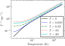
Figure 6: The effect of relaxation parameter $\Gamma$ on the $T^{-1}$ rate. The following parameters are used: $\alpha_{0}=0$, $\Delta=\zeta=10/3\,\textup{cm}^{-1}$, $\omega_{\text{B}}=10\,\textup{cm}^{-1}$, and temperature $T=53.2\,\mathrm{K}$.

The free induction decay like feature of the rate kernel can be modeled by the following equation

$$f(t)=e^{-\Gamma t}\cos(\Omega t),$$ (34)

which has analytical integral: $\int_{0}^{\infty}\differential{t}f(t)=\frac{\Gamma}{\Omega^{2}+\Gamma^{2}}$. Thus, if we consider a relaxation rate to Eq. 32, we would have additional contribution to $T_{1}^{-1}$,

$$\left[\int_{0}^{\infty}\frac{\differential{\omega}}{\pi}J(\omega)\coth{\frac{\beta\omega}{2}}\right]^{2}\frac{2\Gamma}{\Gamma^{2}+\epsilon^{2}}.$$ (35)

Hence, we can neglect the contribution of Eq. 32 to the rate if we have no (FGR) or little (weak coupling regime). Nevertheless, we demonstrate in FIG. 6 that this contribution to the rate cannot be neglected if the relaxation rate $\Gamma$ becomes comparable to $\Omega$. To this end, we argue the FGR treatments for $T_{1}^{-1}$ rate become inadequate when considerable relaxation is introduced by either stronger coupling and/or a mixture of linear and quadratic interaction.

References

- McArdle et al. [2020] S. McArdle, S. Endo, A. Aspuru-Guzik, S. C. Benjamin, and X. Yuan, “Quantum computational chemistry,” Reviews of Modern Physics 92 (2020), 10.1103/revmodphys.92.015003.
- Degen, Reinhard, and Cappellaro [2017] C. Degen, F. Reinhard, and P. Cappellaro, “Quantum sensing,” Reviews of Modern Physics 89 (2017), 10.1103/revmodphys.89.035002.
- Yu et al. [2020a] C.-J. Yu, S. von Kugelgen, M. D. Krzyaniak, W. Ji, W. R. Dichtel, M. R. Wasielewski, and D. E. Freedman, “Spin and phonon design in modular arrays of molecular qubits,” Chemistry of Materials 32, 10200–10206 (2020a).
- Oanta et al. [2022] A. K. Oanta, K. A. Collins, A. M. Evans, S. M. Pratik, L. A. Hall, M. J. Strauss, S. R. Marder, D. M. D’Alessandro, T. Rajh, D. E. Freedman, H. Li, J.-L. Brédas, L. Sun, and W. R. Dichtel, “Electronic spin qubit candidates arrayed within layered two-dimensional polymers,” Journal of the American Chemical Society 145, 689–696 (2022).
- Blais et al. [2021] A. Blais, A. L. Grimsmo, S. Girvin, and A. Wallraff, “Circuit quantum electrodynamics,” Reviews of Modern Physics 93 (2021), 10.1103/revmodphys.93.025005.
- Pelucchi et al. [2021] E. Pelucchi, G. Fagas, I. Aharonovich, D. Englund, E. Figueroa, Q. Gong, H. Hannes, J. Liu, C.-Y. Lu, N. Matsuda, J.-W. Pan, F. Schreck, F. Sciarrino, C. Silberhorn, J. Wang, and K. D. Jöns, “The potential and global outlook of integrated photonics for quantum technologies,” Nature Reviews Physics 4, 194–208 (2021).
- Kloeffel and Loss [2013] C. Kloeffel and D. Loss, “Prospects for spin-based quantum computing in quantum dots,” Annual Review of Condensed Matter Physics 4, 51–81 (2013).
- Aromí et al. [2012] G. Aromí, D. Aguilà, P. Gamez, F. Luis, and O. Roubeau, “Design of magnetic coordination complexes for quantum computing,” Chem. Soc. Rev. 41, 537–546 (2012).
- Coronado [2019] E. Coronado, “Molecular magnetism: from chemical design to spin control in molecules, materials and devices,” Nature Reviews Materials 5, 87–104 (2019).
- Yu et al. [2019] C.-J. Yu, M. D. Krzyaniak, M. S. Fataftah, M. R. Wasielewski, and D. E. Freedman, “A concentrated array of copper porphyrin candidate qubits,” Chemical Science 10, 1702–1708 (2019).
- Yu et al. [2020b] C.-J. Yu, S. von Kugelgen, M. D. Krzyaniak, W. Ji, W. R. Dichtel, M. R. Wasielewski, and D. E. Freedman, “Spin and phonon design in modular arrays of molecular qubits,” Chemistry of Materials 32, 10200–10206 (2020b).
- Moisanu et al. [2023] C. M. Moisanu, R. M. Jacobberger, L. P. Skala, C. L. Stern, M. R. Wasielewski, and W. R. Dichtel, “Crystalline arrays of copper porphyrin qubits based on ion-paired frameworks,” Journal of the American Chemical Society 145, 18447–18454 (2023).
- Graham et al. [2017] M. J. Graham, J. M. Zadrozny, M. S. Fataftah, and D. E. Freedman, “Forging solid-state qubit design principles in a molecular furnace,” Chemistry of Materials 29, 1885–1897 (2017).
- Wasielewski et al. [2020] M. R. Wasielewski, M. D. E. Forbes, N. L. Frank, K. Kowalski, G. D. Scholes, J. Yuen-Zhou, M. A. Baldo, D. E. Freedman, R. H. Goldsmith, T. Goodson, M. L. Kirk, J. K. McCusker, J. P. Ogilvie, D. A. Shultz, S. Stoll, and K. B. Whaley, “Exploiting chemistry and molecular systems for quantum information science,” Nature Reviews Chemistry 4, 490–504 (2020).
- Jarmola et al. [2012] A. Jarmola, V. M. Acosta, K. Jensen, S. Chemerisov, and D. Budker, “Temperature- and magnetic-field-dependent longitudinal spin relaxation in nitrogen-vacancy ensembles in diamond,” Physical Review Letters 108 (2012), 10.1103/physrevlett.108.197601.
- Goldfarb and Stoll [2018] D. Goldfarb and S. Stoll, eds., EPR spectroscopy, eMagRes Books (John Wiley & Sons, Nashville, TN, 2018).
- Tanimura and Kubo [1989] Y. Tanimura and R. Kubo, “Time evolution of a quantum system in contact with a nearly gaussian-markoffian noise bath,” Journal of the Physical Society of Japan 58, 101–114 (1989).
- Tanimura [2020] Y. Tanimura, “Numerically “exact” approach to open quantum dynamics: The hierarchical equations of motion (HEOM),” The Journal of Chemical Physics 153, 020901 (2020).
- Chang and Skinner [1993] T.-M. Chang and J. Skinner, “Non-Markovian population and phase relaxation and absorption lineshape for a two-level system strongly coupled to a harmonic quantum bath,” Physica A: Statistical Mechanics and its Applications 193, 483–539 (1993).
- Blanga and Despósito [1996] L. Blanga and M. Despósito, “Memory effects in the spin relaxation within and without rotating wave approximation,” Physica A: Statistical Mechanics and its Applications 227, 248–261 (1996).
- Xu et al. [2018] R.-X. Xu, Y. Liu, H.-D. Zhang, and Y. Yan, “Theories of quantum dissipation and nonlinear coupling bath descriptors,” The Journal of Chemical Physics 148 (2018), 10.1063/1.4991779.
- xue Xu et al. [2017] R. xue Xu, Y. Liu, H. dao Zhang, and Y. Yan, “Theory of quantum dissipation in a class of non-gaussian environments,” Chinese Journal of Chemical Physics 30, 395–403 (2017).
- Egorov and Skinner [1995] S. A. Egorov and J. L. Skinner, “On the theory of multiphonon relaxation rates in solids,” The Journal of Chemical Physics 103, 1533–1543 (1995).
- Lunghi [2023] A. Lunghi, “Spin-phonon relaxation in magnetic molecules: Theory, predictions and insights,” in Computational Modelling of Molecular Nanomagnets, edited by G. Rajaraman (Springer International Publishing, Cham, 2023) pp. 219–289.
- Leggett et al. [1987] A. J. Leggett, S. Chakravarty, A. T. Dorsey, M. P. A. Fisher, A. Garg, and W. Zwerger, “Dynamics of the dissipative two-state system,” Reviews of Modern Physics 59, 1–85 (1987).
- Yan and Xu [2005] Y. Yan and R. Xu, “QUANTUM MECHANICS OF DISSIPATIVE SYSTEMS,” Annual Review of Physical Chemistry 56, 187–219 (2005).
- Breuer et al. [2016] H.-P. Breuer, E.-M. Laine, J. Piilo, and B. Vacchini, “Colloquium: Non-markovian dynamics in open quantum systems,” Reviews of Modern Physics 88 (2016), 10.1103/revmodphys.88.021002.
- Nitzan [2013] A. Nitzan, Chemical Dynamics in Condensed Phases: Relaxation, Transfer, and Reactions in Condensed Molecular Systems, Oxford Graduate Texts (OUP Oxford, 2013).
- Chen et al. [2023] Z.-H. Chen, Y. Wang, R.-X. Xu, and Y. Yan, “Open quantum systems with nonlinear environmental backactions: Extended dissipaton theory vs core-system hierarchy construction,” The Journal of Chemical Physics 158, 074102 (2023).
- Hu, Xu, and Yan [2010] J. Hu, R.-X. Xu, and Y. Yan, “Communication: Padé spectrum decomposition of fermi function and bose function,” The Journal of Chemical Physics 133 (2010), 10.1063/1.3484491.
- Chen et al. [2022] Z.-H. Chen, Y. Wang, X. Zheng, R.-X. Xu, and Y. Yan, “Universal time-domain prony fitting decomposition for optimized hierarchical quantum master equations,” The Journal of Chemical Physics 156 (2022), 10.1063/5.0095961.
- Zhang and Yan [2016] H.-D. Zhang and Y. Yan, “Kinetic rate kernels via hierarchical liouville–space projection operator approach,” The Journal of Physical Chemistry A 120, 3241–3245 (2016).
- Nakajima [1958] S. Nakajima, “On quantum theory of transport phenomena,” Progress of Theoretical Physics 20, 948–959 (1958).
- Zwanzig [1960] R. Zwanzig, “Ensemble method in the theory of irreversibility,” The Journal of Chemical Physics 33, 1338–1341 (1960).
- Garg, Onuchic, and Ambegaokar [1985] A. Garg, J. N. Onuchic, and V. Ambegaokar, “Effect of friction on electron transfer in biomolecules,” The Journal of Chemical Physics 83, 4491–4503 (1985).
- Tanaka and Tanimura [2009] M. Tanaka and Y. Tanimura, “Quantum dissipative dynamics of electron transfer reaction system: Nonperturbative hierarchy equations approach,” Journal of the Physical Society of Japan 78, 073802 (2009).
- Leggett [1984] A. J. Leggett, “Quantum tunneling in the presence of an arbitrary linear dissipation mechanism,” Physical Review B 30, 1208–1218 (1984).
- Norambuena et al. [2018] A. Norambuena, E. Muñoz, H. T. Dinani, A. Jarmola, P. Maletinsky, D. Budker, and J. R. Maze, “Spin-lattice relaxation of individual solid-state spins,” Physical Review B 97 (2018), 10.1103/physrevb.97.094304.
- Liu et al. [2023] W. Liu, Z.-H. Chen, Y. Su, Y. Wang, and W. Dou, “Predicting rate kernels via dynamic mode decomposition,” The Journal of Chemical Physics 159 (2023), 10.1063/5.0170512.