Range Longest Increasing Subsequence and its Relatives: Beating Quadratic Barrier and Approaching Optimality

Abstract

Longest increasing subsequence ($\mathsf{LIS}$) is a classical textbook problem which is still actively studied in various computational models. In this work, we present a plethora of results for the range longest increasing subsequence problem ($\mathit{Range\mbox{-}LIS}$) and its variants. The input to $\mathit{Range\mbox{-}LIS}$ is a sequence $\mathcal{S}$ of $n$ real numbers and a collection $\mathcal{Q}$ of $m$ query ranges and for each query in $\mathcal{Q}$, the goal is to report the $\mathsf{LIS}$ of the sequence $\mathcal{S}$ restricted to that query. Our two main results are for the following generalizations of the $\mathit{Range\mbox{-}LIS}$ problem:

2D Range Queries:

In this variant of the $\mathit{Range\mbox{-}LIS}$ problem, each query is a pair of ranges, one of indices and the other of values, and we provide an algorithm with running time $\widetilde{O}(mn^{1/2}+n^{3/2}+k)$, where $k$ is the cumulative length of the $m$ output subsequences. This breaks the quadratic barrier of $\widetilde{O}(mn)$ when $m=\Omega(\sqrt{n})$. Previously, the only known result breaking the quadratic barrier was of Tiskin [SODA’10] which could only handle 1D range queries (i.e., each query was a range of indices) and also just outputted the length of the $\mathsf{LIS}$ (instead of reporting the subsequence achieving that length).

Colored Sequences:

In this variant of the $\mathit{Range\mbox{-}LIS}$ problem, each element in $\mathcal{S}$ is colored and for each query in $\mathcal{Q}$, the goal is to report a monochromatic $\mathsf{LIS}$ contained in the sequence $\mathcal{S}$ restricted to that query. For 2D queries, we provide an algorithm for this colored version with running time $\widetilde{O}(mn^{2/3}+n^{5/3}+k)$. Moreover, for 1D queries, we provide an improved algorithm with running time $\widetilde{O}(mn^{1/2}+n^{3/2}+k)$. Thus, we again break the quadratic barrier of $\widetilde{O}(mn)$. Additionally, we prove that assuming the well-known Combinatorial Boolean Matrix Multiplication Hypothesis, that the runtime for 1D queries is essentially tight for combinatorial algorithms.

Our algorithms combine several tools such as dynamic programming (to precompute increasing subsequences with some desirable properties), geometric data structures (to efficiently compute the dynamic programming entries), random sampling (to capture elements which are part of the $\mathsf{LIS}$), classification of query ranges into large $\mathsf{LIS}$ and small $\mathsf{LIS}$, and classification of colors into light and heavy. We believe that our techniques will be of interest to tackle other variants of $\mathsf{LIS}$ problem and other range-searching problems.

1 Introduction

In the longest increasing subsequence ($\mathsf{LIS}$) problem, the input is a sequence of $n$ real numbers $\mathcal{S}=(a_{1},a_{2},\ldots,a_{n})$ and the goal is to report indices $1\leq i_{1}<i_{2}<\cdots<i_{t}\leq n$, for the largest possible value of $t$, such that $a_{i_{1}}<a_{i_{2}}<\cdots<a_{i_{t}}$. The length of the $\mathsf{LIS}$ is then defined to be $t$. For simplicity of discussion, we will assume that all the real numbers in the sequence are distinct. A standard dynamic programming algorithm reports the $\mathsf{LIS}$ in $O(n^{2})$ time, which can be improved to $O(n\log n)$ by performing patience sort [Mal62, Mal63, Arg03, Fre75] or by suitably augmenting a binary search tree which computes each entry in the dynamic programming table in $O(\log n)$ time.

In many applications, such as time-series data analysis, the user might not be interested in the $\mathsf{LIS}$ of the entire sequence. Instead they would like to focus their attention only on a “range” of indices in the sequence. Here are a few examples to illustrate this point.

• Consider a stock $X$ in the trading market. Let the sequence represent the daily price of stock $X$ from 1950 till 2022. Instead of querying for the $\mathsf{LIS}$ of the entire sequence, the user might gain more insights [JMA07, LZZZ17] about the trends of the stock by querying for the $\mathsf{LIS}$ in a range of dates (or time-windows) such as Jan 2020 till March 2020 or Feb 2018 till Dec 2018.

• In modern times, social media platforms are the major source for generating enormous content on the Internet on a minute-to-minute basis. Consider a time-series data with statistics at a fine-grained level (of each minute of the day) about the number of Google searches, number of Tweets posted, number of Amazon purchases, or the number of Instagram posts. Monitoring the $\mathsf{LIS}$ under time-window constraints on such datasets can lead to more insights in understanding the social media usage trends and can also help in detecting abnormalities.

• Popular genome sequencing algorithms identify high scoring segment pairs (HSPs) between a query transcript sequence and a long reference genomic sequence in order to obtain a global alignment, and this amounts to computing the $\mathsf{LIS}$ in the reference genome [AGM⁺90, Zha03, AGH⁺04]. Typically many queries are made (corresponding to various transcripts/proteins) w.r.t. the same reference genomic sequence, and this can be modeled as range queries to compute the $\mathsf{LIS}$.

Recently, in the theoretical computer science community, there has been a lot of interest in the dynamic $\mathsf{LIS}$ problem [MS20, KS21, GJ21b], where the goal is to maintain exact or approximate $\mathsf{LIS}$ under insertion and deletion of elements. Interestingly, an important subroutine which shows up is the computation of $\mathsf{LIS}$ of a given range of elements in the sequence. For example, Gawrychowski and Janczewski [GJ21b] design a dynamic algorithm to quickly compute the approximate $\mathsf{LIS}$ for any range of indices in $\mathcal{S}$. In fact, Gawrychowski and Janczewski go further and design a dynamic algorithm which maintains the approximate $\mathsf{LIS}$ for a special class of dyadic rectangles where the query is an axis-aligned rectangle in 2D and the goal is to compute the approximate $\mathsf{LIS}$ of the 2D points (from the above mapping) which lie inside the rectangle.

Motivated by this, in this paper we study several natural variants of the $\mathsf{LIS}$ problem where the 1D queries impose restriction on the range of the indices and the 2D queries impose range restriction on both the indices and the values in the sequence.

Problem-I: One dimensional range $\mathsf{LIS}$ problem.

The first problem is the 1D range longest increasing subsequence problem ($\mathit{1D\mbox{-}Range\mbox{-}LIS}$). In the $\mathit{1D\mbox{-}Range\mbox{-}LIS}$ problem, we are given as input a sequence $\mathcal{S}=(a_{1},a_{2},\ldots,a_{n})$ of $n$ real numbers and a collection $\mathcal{Q}$ of $m$ query ranges, where each $q\in\mathcal{Q}$ is a range (or an interval) $[x_{1},x_{2}]\subseteq[1,n]$. For each $q=[x_{1},x_{2}]\in\mathcal{Q}$, the goal is to report the $\mathsf{LIS}$ of the sequence $\mathcal{S}\cap[x_{1},x_{2}]=(a_{x_{1}},a_{x_{1}+1}\ldots,a_{x_{2}-1},a_{x_{2}})$ (i.e., the output must be the longest increasing subsequence in $\mathcal{S}\cap[x_{1},x_{2}]$). The length of the $\mathsf{LIS}$ of the sequence $\mathcal{S}\cap q$ is denoted by $\mathsf{LIS}(\mathcal{S}\cap q)$.

A straightforward approach to solve the $\mathit{1D\mbox{-}Range\mbox{-}LIS}$ problem would involve no preprocessing: for each range $[x_{1},x_{2}]$ in $\mathcal{Q}$, we will retrieve the elements $a_{x_{1}},a_{x_{1}+1}\ldots,a_{x_{2}-1},a_{x_{2}}$ and report their $\mathsf{LIS}$. This would require $\Omega(mn\log n)$ time in the worst-case (for instance when many of the ranges in $\mathcal{Q}$ are of $\Omega(n)$ length). This leads to the following natural question of beating the quadratic runtime of $O(mn\log n)$ for $\mathit{1D\mbox{-}Range\mbox{-}LIS}$:

Is there an algorithm that can solve $\mathit{1D\mbox{-}Range\mbox{-}LIS}$ in sub-quadratic runtime?

In a remarkable work, Tiskin [Tis08a, Tis08b, Tis10] broke the quadratic barrier, by designing an $O((n+m)\log n)$ time algorithm, albeit for the computationally easier length version of the $\mathit{1D\mbox{-}Range\mbox{-}LIS}$ problem, in which for all $q\in\mathcal{Q}$, the goal is to only output the length of the $\mathsf{LIS}$ in the range $q$ (i.e., $\mathsf{LIS}(\mathcal{S}\cap q)$). The algorithm designed by Tiskin is tailored to handle the length version of the $\mathit{1D\mbox{-}Range\mbox{-}LIS}$ problem and to the best of our knowledge, does not readily adapt to the reporting version (this is further discussed in Appendix A).

In this paper, we beat the quadratic time barrier for the reporting version of $\mathit{1D\mbox{-}Range\mbox{-}LIS}$ problem when $m$ is roughly $\Omega(\sqrt{n})$. We obtain the following result.

Theorem 1.

There is a randomized algorithm to answer the reporting version of the $\mathit{1D\mbox{-}Range\mbox{-}LIS}$ problem in $O(\sqrt{n}(m+n)(\log n)^{3}+k)$ time, where $k$ is the cumulative length of the $m$ output subsequences. The bound on the running time and the correctness of the solution holds with high probability.

Problem-II: Two dimensional range $\mathsf{LIS}$ problem.

The second problem is the 2D range longest increasing subsequence problem ($\mathit{2D\mbox{-}Range\mbox{-}LIS}$) which is a natural generalization of the $\mathit{1D\mbox{-}Range\mbox{-}LIS}$ problem. As before, we are given as input a sequence $\mathcal{S}=(a_{1},a_{2},\ldots,a_{n})$. Consider a mapping where the $i^{\text{th}}$ element $a_{i}\in\mathcal{S}$ is mapped to a 2D point $p_{i}=(i,a_{i})$. Let $\mathcal{P}=\{p_{1},p_{2},\ldots,p_{n}\}$ be a collection of these $n$ points. We are also given as input a collection $\mathcal{Q}$ of $m$ query ranges, where each range in $\mathcal{Q}$ is an axis-aligned rectangle in 2D. For each $q\in\mathcal{Q}$, the goal is to report the $\mathsf{LIS}$ of $\mathcal{P}\cap q$, i.e., the points of $\mathcal{P}$ lying inside $q$. See Figure 1(a) for an example.

Once again the naive approach to solve the problem would take $O(mn\log n)$ time, where for each range $q\in\mathcal{Q}$, we will scan the points in $\mathcal{P}$ to filter out the points lying inside $q$ and then compute their $\mathsf{LIS}$. One might be tempted to use orthogonal range searching data structures [AAL09, AE98, CLP11, NR23, BCKO08] to efficiently report $\mathcal{P}\cap q$, but in the worst-case we could have many queries with $|\mathcal{P}\cap q|=\Omega(n)$. In this paper, even for the $\mathit{2D\mbox{-}Range\mbox{-}LIS}$ problem, we succeed to beat the quadratic time barrier when $m$ is roughly $\Omega(\sqrt{n})$. We obtain the following result.

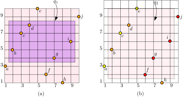
Figure 1: (a) Each element in the sequence $\mathcal{S}=(3,5,7,8,10,2,4,1,6,9)$ is mapped to a 2D point. For example, the element $7$ is mapped to $c=(3,7)$. The $\mathit{2D\mbox{-}Range\mbox{-}LIS}$ of the points lying inside $q_{1}$ is $(b,c,d)$. (b) The same input sequence $\mathcal{S}=(3,5,7,8,10,2,4,1,6,9)$ is shown here. The set of colors $\mathcal{C}=\{\text{orange, yellow, red}\}$. Points $b,d\text{ and }h$ have orange color, points $a,c\text{ and }e$ have yellow color, and points $f,g,i\text{ and }j$ have red color. The $\mathit{Colored\mbox{-}2D\mbox{-}Range\mbox{-}LIS}$ of the points lying inside $q_{2}$ (the shaded region) is red color realized by the sequence $(f,g,i)$.

Theorem 2.

There is a randomized algorithm to answer the reporting version of $\mathit{2D\mbox{-}Range\mbox{-}LIS}$ problem in $O(\sqrt{n}(m+n)(\log n)^{5}+k)$ time, where $k$ is the cumulative length of the $m$ output subsequences. The bound on the running time and the correctness of the solution holds with high probability.

Problem-III: Colored 1D range $\mathsf{LIS}$ problem.

In the geometric data structures literature, colored range searching [KN11, NV13, PTS⁺14, Mut02, LPS08, KSV06, BKMT95, AGM02, GJS95, JL93, LP12, Nek14, SJ05, GJRS18] is a well-studied generalization of traditional range searching problems. In the colored setting, the geometric objects are partitioned into disjoint groups (or colors), and given a query region $q$, the typical goal is to efficiently report [CHN20, CN20, CH21, LvW13], or count [KRSV07], or approximately count [Rah17] the number of colors intersecting $q$, or find the majority color inside $q$ [CDL⁺14, KMS05].

In the same spirit, we study the colored 1D range longest increasing subsequence problem ($\mathit{Colored\mbox{-}1D\mbox{-}Range\mbox{-}LIS}$). In addition to the sequence $\mathcal{S}$ and 1D range queries $\mathcal{Q}$ given as input to the $\mathit{1D\mbox{-}Range\mbox{-}LIS}$ problem, in the $\mathit{Colored\mbox{-}1D\mbox{-}Range\mbox{-}LIS}$ problem we are additionally given a coloring of $\mathcal{S}$ using the color set $\mathcal{C}$. Each element $a_{i}\in\mathcal{S}$ has a color chosen from $\mathcal{C}$ (the corresponding 2D point $p_{i}$ also has the same color). For all $c\in\mathcal{C}$, let $\mathcal{P}_{c}\subseteq\mathcal{P}$ denote the set of points with color $c$ and for any $q\in\mathcal{Q}$, with a slight abuse of notation, we will use $\mathsf{LIS}(\mathcal{P}_{c}\cap q)$ to denote the length of the $\mathsf{LIS}$ of $\mathcal{P}_{c}\cap q$. Moreover, we say a subsequence is monochromatic, if all the elements in the subsequence have the same color. For each $q\in\mathcal{Q}$, the goal is then to report the longest monochromatic increasing subsequence whose length is equal to $\underset{c\in C}{\max}\ \mathsf{LIS}(\mathcal{P}_{c}\cap q)$. See Figure 1(b) for an example in 2D. We obtain the following result.

Theorem 3.

There is a randomized algorithm to answer the reporting version of the $\mathit{Colored\mbox{-}1D\mbox{-}Range\mbox{-}LIS}$ problem in $O(\sqrt{n}(m+n)(\log n)^{3}+k)$ time, where $k$ is the cumulative length of the $m$ output subsequences. The bound on the running time and the correctness of the solution holds with high probability.

We complement the above result with a conditional lower bound that indicates that the above runtime for $\mathit{Colored\mbox{-}1D\mbox{-}Range\mbox{-}LIS}$ might be (near) optimal.

Theorem 4.

Assuming the Combinatorial Boolean Matrix Multiplication Hypothesis, for every $\varepsilon>0$, there is no combinatorial algorithm to answer the reporting version of the $\mathit{Colored\mbox{-}1D\mbox{-}Range\mbox{-}LIS}$ problem in $O(n^{0.5-\varepsilon}\cdot(m+n))$ time. The lower bound continues to hold even when we are only required to report the color of the longest monochromatic increasing subsequence for each range query.

The Combinatorial Boolean Matrix Multiplication Hypothesis ($\mathsf{CBMMH}$) roughly asserts that Boolean matrix multiplication of two $\sqrt{n}\times\sqrt{n}$ matrices cannot be computed by any combinatorial algorithm running in time $n^{1.5-\varepsilon}$, for any constant $\varepsilon>0$ (see Definition 3 for a formal statement). Here “combinatorial algorithm” is typically defined as “non-Strassen-like algorithm” (as defined in [BDHS13]), and this captures all known fast matrix multiplication algorithms.

While $\mathsf{CBMMH}$ is widely explored since the 1990s [Sat94, Lee02], there is no strong consensus in the computer science community about its plausibility. In a recent breakthrough, Abboud et al. [AFK⁺24], have come tantalizingly close to even refuting it. All that said, $\mathsf{CBMMH}$ remains a widely used hypothesis for proving conditional lower bounds [RZ11, AW14, HKNS15]. At the very least, Theorem 4 provides evidence that any algorithm for $\mathit{Colored\mbox{-}1D\mbox{-}Range\mbox{-}LIS}$ that is significantly faster than the runtime given in Theorem 3, must be highly non-trivial!

The proof of Theorem 4 follows as a simple consequence of a $\mathsf{CBMMH}$ based conditional lower bound in [CDL⁺14] for computing the mode of a sequence subject to range queries.

Problem-IV: Colored 2D range $\mathsf{LIS}$ problem.

The most general problem that we study in this paper is the colored 2D range longest increasing subsequence problem ($\mathit{Colored\mbox{-}2D\mbox{-}Range\mbox{-}LIS}$). The queries in $\mathcal{Q}$ will be axis-aligned rectangles. For each $q\in\mathcal{Q}$, the goal is then to report the longest monochromatic increasing subsequence which attains $\underset{c\in C}{\max}\ \mathsf{LIS}(\mathcal{P}_{c}\cap q)$. See Figure 1(b) for an example. We obtain the following result.

Theorem 5.

There is a randomized algorithm to answer the reporting version of the $\mathit{Colored\mbox{-}2D\mbox{-}Range\mbox{-}LIS}$ problem in $O(n^{2/3}(m+n)(\log n)^{5}+k)$ time, where $k$ is the cumulative length of the $m$ output subsequences. The bound on the running time and the correctness of the solution holds with high probability.

We remark that the conditional lower bound of Theorem 4 continues to hold here too.

In Table 1, we have summarized the state-of-the-art upper and (conditional) lower bounds for the various variants of $\mathit{Range\mbox{-}LIS}$ discussed in this paper.

Problem	Upper Bound	Lower Bound
1D-Range LIS	$O(\sqrt{n}(m+n)(\log n)^{3}+k)$	$\Omega(m+n+k)$
	(Theorem 1)	(Trivial)
2D-Range LIS	$O(\sqrt{n}(m+n)(\log n)^{5}+k)$	$\Omega(m+n+k)$
	(Theorem 2)	(Trivial)
Colored 1D-Range LIS	$O(\sqrt{n}(m+n)(\log n)^{3}+k)$	$\Omega\left(n^{1/2-o(1)}(m+n)\right)$
	(Theorem 3)	(Theorem 4)
Colored 2D-Range LIS	$O(n^{2/3}(m+n)(\log n)^{5}+k)$	$\Omega\left(n^{1/2-o(1)}(m+n)\right)$
	(Theorem 5)	(Theorem 4)

Table 1: State-of-the-art upper and lower bounds are listed for the variants of $\mathit{Range\mbox{-}LIS}$ problem considered in this paper. In the table, all upper bounds from this paper are randomized, and all lower bounds from this paper are conditional and only against combinatorial algorithms. Also, recall that $n$ is the length of input sequence, $m$ is the number of range queries, and $k$ is the cumulative size of the $m$ outputs.

1.1 Related Works

To the best of our knowledge, there is no prior work on the reporting version of $\mathit{Range\mbox{-}LIS}$, and we have elaborated in Appendix A the result of Tiskin [Tis08a, Tis08b, Tis10] on the length version of $\mathit{1D\mbox{-}Range\mbox{-}LIS}$ (which to the best of our knowledge, cannot be adpated to efficiently answer the reporting version of $\mathit{Range\mbox{-}LIS}$ problem, which is the focus of this paper). Therefore, for the rest of this subsection, we list works on the $\mathsf{LIS}$ problem in some popular settings/models.

In the Dynamic $\mathsf{LIS}$ problem we need to maintain the length of $\mathsf{LIS}$ of an array under insertion and deletion. The $\mathsf{LIS}$ problem in the dymanic setting was initiated by Mitzenmacher and Seddighin [MS20]. In [GJ21b], an algorithm running in $O(\varepsilon^{-5}(\log n)^{11})$ time and providing $(1+\varepsilon)$-approximation was presented (this approximation algorithm can be adapted to approximate the $\mathit{Range\mbox{-}LIS}$ problem in the dynamic setting), and in [KS21] a randomized exact algorithm with the update and query time $\widetilde{O}(n^{4/5})$ was provided. Finally, in [GJ21a], the authors provide conditional polynomial lower bounds for exactly solving $\mathit{Range\mbox{-}LIS}$ in the dynamic setting.

In the streaming model, computing the $\mathsf{LIS}$ requires $\Omega(n)$ bits of space [GJKK07], so it is natural to resort to approximation algorithms. In [GJKK07] is a deterministic $(1+\varepsilon)$-approximation in $O(\sqrt{n/\varepsilon})$ space for $\mathsf{LIS}$ problem, and this was shown to be optimal [EJ08, GG10]. We remark here that the $\mathsf{LIS}$ problem has also been implicitly studied in the streaming algorithms literature as estimating the sortedness of an array [AJKS02, LNVZ06, GJKK07, SW07].

In the setting of sublinear time algorithms, the authors of [SS17] showed how to approximate the length of the $\mathsf{LIS}$ to within an additive error of $\varepsilon\cdot n$, for an arbitrary $\varepsilon\in(0,1)$, with $(1/\varepsilon)^{1/\varepsilon}\cdot(\log n)^{O(1)}$ queries. Denoting the length of $\mathsf{LIS}$ by $\ell$, in [RSSS19] the authors designed a non-adaptive $O(\lambda^{-3})$-multiplicative factor approximation algorithm, where $\lambda=\ell/n$, with $O(\sqrt{n}/\lambda^{7})$ queries (and also obtained different tradeoffs between the dependency on $\lambda$ and $n$). In [NV21], the authors proved that adaptivity is essential in obtaining polylogarithmic query complexity for the $\mathsf{LIS}$ problem. Recently, for any $\lambda=o(1)$, in [ANSS22] a (randomized) non-adaptive $1/\lambda^{o(1)}$-multiplicative factor approximation algorithm was provided with $n^{o(1)}/\lambda$ running time.

In the read-only random access model, the authors of [KOO⁺18] showed how to find the length of $\mathsf{LIS}$ in $O((n^{2}/s)\log n)$ time and only $O(s)$ space, for any parameter $\sqrt{n}\leq s\leq n$.

Range-aggregate queries have traditionally been well-studied in the database community and the computational geometry community. See the survey papers [AE98, RT19, GJRS18]. In a typical range-aggregate query, the input is a collection of points in a $d$-dimensional space, and the user specifies a range query (such as an axis-aligned rectangle, or a disk, or a halfspace), and the goal is to compute an informative summary of the subset of points which lie inside the range query, such as the top-$k$ points [RT15, RT16, ABZ11, BFGLO09], a random subset of $k$ points [Tao22, HQT14], reporting or counting colors or groups [CN20, CHN20, Rah21], statistics such as mode, median [BGJS11], or sum, the closest pair of points [XLRJ20, XLRJ22], and the skyline points [BL14, RJ12].

In an orthogonal range-max problem, the input is a set $\mathcal{P}$ of $n$ points in $d$-dimensional space. Each point in $\mathcal{P}$ has a weight associated with it. Preprocess $\mathcal{P}$ into a data structure, so that given an axis-parallel box $q$, the goal is to report the point in $\mathcal{P}\cap q$ with the largest weight. In this work, we will use vanilla range trees from the textbook [BCKO08] to answer range-max queries (since the goal of this work is not to shave polylogarithmic factors). The preprocessing time to build a vanilla range tree is $O(n\log^{d}n)$ and the query time is $O(\log^{d}n)$.

1.2 Our first technique: Handling small $\mathsf{LIS}$

We design a general technique to obtain all our upper bounds. For the sake of simplicity, we will give an overview of the general technique for the simplest case of $\mathit{1D\mbox{-}Range\mbox{-}LIS}$ (Theorem 1) which is in 1D and does not involve colors.

Our strategy to solve the $\mathit{1D\mbox{-}Range\mbox{-}LIS}$ problem is the following. Consider an integer parameter $\tau\in[1,n]$. For the $\mathit{1D\mbox{-}Range\mbox{-}LIS}$ problem, $\tau$ is set to $\sqrt{n}$. We will design two different techniques. The first technique is deterministic and reports the correct answer if $\mathsf{LIS}(\mathcal{S}\cap q)\leq\tau$. If $\mathsf{LIS}(\mathcal{S}\cap q)>\tau$, then correctness is not guaranteed. The second technique is randomized and reports the correct answer with high probability if $\mathsf{LIS}(\mathcal{S}\cap q)\geq\tau$. If $\mathsf{LIS}(\mathcal{S}\cap q)<\tau$, then correctness is not guaranteed. As such, for each $q\in\mathcal{Q}$, with high probability, the correct result is obtained by one of the two algorithms.

In this subsection, we will give an overview of the first technique for $\mathit{1D\mbox{-}Range\mbox{-}LIS}$. In our discussion we will use the terms element and point interchangeably. As discussed before, the $i^{\text{th}}$ element in sequence $\mathcal{S}$ is equivalent to the 2D point $(i,a_{i})$ in $\mathcal{P}$. Consider the special case where there is a vertical line with $x$-coordinate $x^{*}$ such that each query range in $\mathcal{Q}$ contains $x^{*}$ (we will show later in Section 2 how to remove the assumption).

Idea-1: Lowest peaks and highest bases.

Please refer to Figure 2(i) where eighteen points are shown. Chain $C_{1}$ and chain $C_{2}$ are increasing sequences to the left of $x^{*}$ and both have length four. Our first observation is that it we are allowed to store either $C_{1}$ or $C_{2}$, then it would be wiser to store $C_{2}$. The reason is that $C_{2}$ can “stitch” itself with chain $C_{3}$ and $C_{4}$, to form an increasing subsequence of length six and eight, respectively. On the other hand, $C_{1}$ cannot stitch itself with $C_{3}$ or $C_{4}$ to form a larger increasing subsequence. Analogously, between chains $C_{4}$ and $C_{5}$, we will prefer $C_{4}$ since it can stitch with $C_{2}$, whereas $C_{5}$ cannot stitch with any chain to the left of $x^{*}$. In fact, the $\mathsf{LIS}$ of the eighteen points is realised by the chain $C_{2}\cup C_{4}$ with length eight. This motivates the definition of lowest peak and highest base.

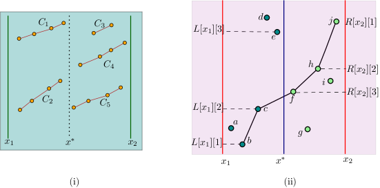
Figure 2: (i) An example with eighteen points and five chains is shown. (ii) An example with ten points. The query is the range $[x_{1},x_{2}]$. In the range $[x_{1},x^{*}]$, the sequence with the lowest peak of length one is $(b)$, of length two is $(b,c)$ or $(a,c)$, of length three is $(b,c,e)$ or $(a,c,e)$. In the range $[x^{*},x_{2}]$, the sequence with the highest base of length one is $(j)$, of length two is $(h,j)$, of length three $(f,h,j)$ or $(f,i,j)$. The $\mathsf{LIS}$ of points in the range $[x_{1},x_{2}]$ is five and the corresponding compatible pair is $(L[x_{1}][2],R[x_{2}][3])$.

For an increasing subsequence $S\in\mathcal{S}$, we define peak (resp., base) to be the last (resp., first) element in $S$. The algorithm will store two $2$-dimensional arrays:

Array $L$:

For all integers $1\leq x_{1}\leq x^{*}$ and for all $1\leq\alpha\leq\tau$, among all increasing subsequences of length $\alpha$ in the range $[x_{1},x^{*}]$, let $S$ be the subsequence with the lowest peak. Then $L[x_{1}][\alpha]$ stores the value of the last element in $S$.

Array $R$:

For all integers $x^{*}<x_{2}\leq n$ and for all $1\leq\beta\leq\tau$, among all increasing sequences of length $\beta$ in the range $(x^{*},x_{2}]$, let $S$ be the subsequence with the highest base. Then $R[x_{2}][\beta]$ stores the value of the first element in $S$.

For example, in Figure 2(i), for the range $[x_{1},x^{*}]$ and $\alpha=4$, the chain $C_{2}$ is the subsequence with the lowest peak; and for $(x^{*},x_{2}]$ and $\alpha=4$, chain $C_{4}$ is the subsequence with the highest base. Efficient computation of the $O(n\tau)$ entries in arrays $L$ and $R$ will be discussed later.

A pair $(L[x_{1}][\alpha],R[x_{2}][\beta])$ is defined to be compatible if $L[x_{1}][\alpha]<R[x_{2}][\beta]$, i.e., it is possible to “stitch” the sequences corresponding to $L[x_{1}][\alpha]$ and $R[x_{2}][\beta]$ to obtain an increasing sequence of length $\alpha+\beta$. For a query range $q=[x_{1},x_{2}]$, our goal is to find the compatible pair $(L[x_{1}][\alpha],R[x_{2}][\beta])$ which maximizes the value of $\alpha+\beta$, i.e.,

$$\mathsf{LIS}(\mathcal{S}\cap[x_{1},x_{2}])=\max_{\alpha,\beta}\{\alpha+\beta\mid L[x_{1}][\alpha]<R[x_{2}][\beta]\}.$$

Idea-2: Monotone property of peaks and bases.

For a given query $q=[x_{1},x_{2}]$, a naive approach is to inspect all pairs of the form $(L[x_{1}][\alpha],R[x_{2}][\beta])$, for all $1\leq\alpha,\beta\leq\tau$, and then pick a compatible pair which maximizes the value of $\alpha+\beta$. The number of pairs inspected is $\Theta(\tau^{2})$ which we cannot afford. However, the following monotone property will help in reducing the number of pairs inspected to $O(\tau\log\tau)$:

• For a fixed value of $x_{1}$, the value of $L[x_{1}][\alpha]$ increases as the value of $\alpha$ increases, i.e., for any $1\leq\alpha\leq\alpha^{\prime}\leq\tau$, we have $L[x_{1}][\alpha]\leq L[x_{1}][\alpha^{\prime}]$.

• Analogously, for a fixed value of $x_{2}$, the value of $R[x_{2}][\beta]$ decreases as the value of $\beta$ increases, i.e., for any $1\leq\beta\leq\beta^{\prime}\leq\tau$, we have $R[x_{2}][\beta]\geq R[x_{2}][\beta^{\prime}]$.

See Figure 2(ii) for an example where $L[x_{1}][\alpha]$ values are increasing with increase in $\alpha$ and $R[x_{2}][\beta]$ values are decreasing with increase in $\beta$. For each $1\leq i\leq\tau$, the largest $\beta_{i}$ for which $(L[x_{1}][i],R[x_{2}][\beta_{i}])$ is compatible can be found in $O(\log\tau)$ time by doing a binary search on the monotone sequence $(R[x_{2}][1],R[x_{2}][2],\ldots,R[x_{2}][\tau])$. Finally, report $\max_{i}(i+\beta_{i})$ as the length of the $\mathsf{LIS}$ for $\mathcal{S}\cap q$. Overall, the time taken to answer the $m$ query ranges will be $O(m\tau\log\tau)$.

Idea-3: Pivot points and dynamic programming.

Now the key task is to design a preprocessing algorithm which can quickly compute each entry in the two-dimensional arrays $L$ and $R$. We will look at $R$ and an analogous discussion will hold for $L$. Assume that we have computed the value of $R[x_{2}-1][\beta]$ and would like to next compute $R[x_{2}][\beta]$. Let $p_{x_{2}}=(x_{2},a_{x_{2}})$ be the point with $x$-coordinate $x_{2}$. which is encountered when we move the vertical line from $x_{2}-1$ to $x_{2}$.

Formally, we claim that the value of $R[x_{2}][\beta]$ is higher than $R[x_{2}-1][\beta]$ if and only if there is an increasing subsequence with the following three properties: (i) the subsequence length is $\beta$, (ii) the base of the subsequence is higher than $R[x_{2}-1][\beta]$, and (iii) the last point in the subsequence is $p_{x_{2}}$. Please refer to Figure 3 for an example.

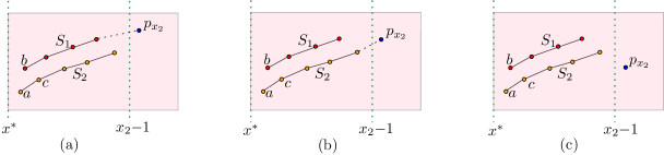
Figure 3: Two sequences $S_{1}$ and $S_{2}$ lie to the left of the vertical line $x_{2}-1$. The value of $R[x_{2}-1][5]$ is realized by the $y$-coordinate of point $a$. In (a) and (b), we have $R[x_{2}][5]>R[x_{2}-1][5]$, and in (c), we have $R[x_{2}][5]=R[x_{2}-1][5]$. In case (a), point $p_{x_{2}}$ stitches with $S_{1}$ to obtain a subsequence of length five with with higher base than $a$. In case (b), by stitching point $p_{x_{2}}$ with $S_{2}$ and removing point $a$, we obtain a subsequence of length five and it has a higher base than $a$.

We define $p_{x_{2}}$ to be a pivot point. Now to efficiently compute $R[x_{2}][\beta]$, we will need the support of another two-dimensional array $B$ defined as follows: among all increasing subsequences of length $\beta$ in the range $(x^{*},x_{2}]$ containing pivot point $p_{x_{2}}$ as the last element, let $S$ be the subsequence with the highest base. Then $B[x_{2}][\beta]$ is defined to be the value of the first element in $S$. In Figure 3(a) and Figure 3(b), $B[x_{2}][5]$ is realized by the $y$-coordinate of $b$ and $c$, respectively. As a result, we can succinctly encode the three properties stated above as follows:

$$R[x_{2}][\beta]\leftarrow\max\{R[x_{2}{-}1][\beta],B[x_{2}][\beta]\}.$$

In other words, an increasing sequence of length $\beta$ in the interval $(x^{*},x_{2}]$ with the highest base will either contain the pivot element $p_{x_{2}}$ or not. The first term (i.e., $R[x_{2}{-}1][\beta]$) captures the case where $p_{x_{2}}$ is not included, whereas the second term (i.e., $B[x_{2}][\beta]$) captures the case where $p_{x_{2}}$ is included. As such, the task of efficiently computing $R$ has been reduced to the task of efficiently computing $B$.

Idea-4: 2D range-max data structure.

The final step is to compute each entry in $B$ in polylogarithmic time. The entries will be computed in increasing values of $\beta$. Assume that the entries corresponding to sequences of length at most $\beta{-}1$ have been computed. Then the entries $B[x_{2}][\beta]$’s can be reduced to entries of $B[\cdot][\beta-1]$’s as follows:

$$B[x_{2}][\beta]=\begin{cases}a_{x_{2}},\quad\text{ if $\beta=1$;}\\ -\infty,\ \ \ \text{if $a_{i}>a_{x_{2}}$ for all $x^{*}<i<x_{2}$;}\\ \max\{B[i][\beta{-}1]\ |\ x^{*}<i<x_{2}\text{ and }a_{i}<a_{x_{2}}\},\quad\text{otherwise}.\end{cases}$$

We will efficiently compute $B[x_{2}][\beta]$’s by constructing a data structure which can answer 2D range-max queries. In a 2D range-max query, we are given $n$ weighted points $\mathcal{P}$ in 2D. Each point is associated with a weight. For each point $p_{i}=(i,a_{i})\in\mathcal{P}$, given a query region of the form $q^{\prime}=(-\infty,i)\times(-\infty,a_{i})$, the goal is to report the point in $\mathcal{P}\cap q^{\prime}$ with the maximum weight. The 2D range-max problem can be solved in $O(n\log n)$ time (via reduction to the so-called 2D orthogonal point location problem [ST86]).

Now with each point $p_{i}\in\mathcal{P}$, we associate the weight $B[i][\beta-1]$ and build a 2D range-max data structure. For each point $p_{x_{2}}=(x_{2},a_{x_{2}})\in\mathcal{P}$, the point in $\mathcal{P}\cap(-\infty,x_{2})\times(-\infty,a_{x_{2}})$ with the maximum weight is reported. If point $p_{i}$ is reported, then set $B[x_{2}][\beta]=B[i][\beta-1]$. The correctness follows from the third case in the above dynamic programming. Since $\beta\leq\tau$, the time taken to construct $B$ is $O(\tau)\times O(n\log n)=O(n\tau\log n)$.

Therefore, the overall time taken by this technique to answer $\mathit{1D\mbox{-}Range\mbox{-}LIS}$ will be $\widetilde{O}(m\tau+n\tau+k)=\widetilde{O}(m\sqrt{n}+n\sqrt{n}+k)$ by setting $\tau\leftarrow\sqrt{n}$.

Idea-5: Generalizing $L$ and $R$ to handle $\mathit{2D\mbox{-}Range\mbox{-}LIS}$.

We briefly describe the challenge arising while handling $\mathit{2D\mbox{-}Range\mbox{-}LIS}$ where the queries are axis-parallel rectangles. The definition of highest bases and lowest peak fail to be directly useful. For example, see Figure 4, where $\mathsf{LIS}(\mathcal{P}\cap q)$ is equal to five, and is realized by stitching $S_{2}$ and $S_{3}$. However, $L[x_{1}][3]$ will correspond to the sequence $S_{1}$ and $R[x_{2}][2]$ will correspond to the sequence $S_{4}$, both of which lie completely outside $q$.

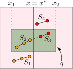
Figure 4: Four increasing subsequences lying in the range $[x_{1},x_{2}]\times(-\infty,+\infty)$.

The key observation in the 2D setting is that for an increasing subsequence $S$ and a query rectangle $q=[x_{1},x_{2}]\times[y_{1},y_{2}]$, if the first and the last point of $S$ lie inside $q$, then all the points of $S$ lie inside $q$. Accordingly, we generalize the definitions of $L$ and $R$. Specifically, in the 2D setting, $R$ takes two arguments, the query $q$ and an integer $\beta$, and is defined as follows:

$$R(q,\beta)\leftarrow\max_{p_{i}=(i,a_{i})}\{B[i][\beta]\mid p_{i}\in q,i>x^{*}\text{ and }B[i][\beta]>y_{1}\}.$$

For example, in Figure 4, the new definition of $R(q,2)$ ensures that the sequence $S_{3}$ gets captured instead of $S_{4}$. We construct $L$ analogously. Note that in the 1D setting, $L$ and $R$ were explicitly computed. However, in the 2D setting, the number of combinatorially different axis-parallel rectangles is significantly more than our time budget. Therefore, $L$ and $R$ cannot be pre-computed and stored. Instead, for all $1\leq\alpha\leq\tau$ (resp., $1\leq\beta\leq\tau$), we will compute $L(q,\alpha)$ (resp., $R(q,\beta)$) during the query algorithm in $O(\tau\cdot\text{polylog }n)$ time.

1.3 Our second technique: Handling large $\mathsf{LIS}$

Now we give an overview of our second technique. If $\mathsf{LIS}(\mathcal{S}\cap q)\geq\tau$, then this technique will report the answer correctly with high probability.

Idea-1: Stitching elements.

One challenge with the $\mathsf{LIS}$ problem is that it is not decomposable. Consider a query range $q=[x_{1},x_{2}]\times(-\infty,+\infty)$ and an $x^{*}$ such that $x_{1}<x^{*}<x_{2}$. Let $q_{\ell}=[x_{1},x^{*}]\times(-\infty,+\infty)$ and $q_{r}=(x^{*},x_{2}]\times(-\infty,+\infty)$ such that $q=q_{\ell}\cup q_{r}$. Then the $\mathsf{LIS}$ of $\mathcal{P}\cap q$ need not be the concatenation of the $\mathsf{LIS}$ of $\mathcal{P}\cap q_{\ell}$ and the $\mathsf{LIS}$ of $\mathcal{P}\cap q_{r}$, since the rightmost point in the $\mathsf{LIS}$ of $\mathcal{P}\cap q_{\ell}$ might have a larger value than the leftmost point in the $\mathsf{LIS}$ of $\mathcal{S}\cap q_{r}$.

However, suppose an oracle reveals that point $p_{i}\in\mathcal{P}$ lies in the $\mathsf{LIS}$ of range $q=[x_{1},x_{2}]\times(-\infty,+\infty)$. Then we claim that the problem becomes decomposable. We will define some notation before proceeding. For a point $p_{i}=(i,a_{i})\in\mathcal{P}$ corresponding to an element $a_{i}\in\mathcal{S}$, define the north-east region of $p_{i}$ as $NE(p_{i})=\{(x,y)\mid x\geq i\text{ and }y\geq a_{i}\}$. Analogously, define the north-west, the south-west and the south-east region of $p_{i}$ which are denoted by $NW(p_{i}),SW(p_{i})\text{ and }SE(p_{i})$, respectively. Then it is easy to observe that,

$$\mathsf{LIS}(\mathcal{P}\cap q)=\mathsf{LIS}(\mathcal{P}\cap q\cap NE(p_{i}))+\mathsf{LIS}(\mathcal{P}\cap q\cap SW(p_{i}))-1.$$ (1)

See Figure 5 for an example. In other words, knowing that $p_{i}$ belongs to the $\mathsf{LIS}$ decomposes the original $\mathsf{LIS}$ problem into two $\mathsf{LIS}$ sub-problems which can be computed independently. In such a case, we refer to point $p_{i}$ as a stitching element, which is formally defined below.

Definition 1.

(Stitching element) For a range $q$, fix any $\mathsf{LIS}$ of $\mathcal{P}\cap q$ and call it $S$. Then each element in $S$ is defined to be a stitching element w.r.t. $q$.

The goal of our algorithm is to:

Construct a small-sized set $\mathcal{R}\subseteq\mathcal{P}$ such that, for any $q\in\mathcal{Q}$, at least one stitching element w.r.t. $q$ is contained in $\mathcal{R}\cap q$.

For each $p_{i}\in\mathcal{R}$, in the preprocessing phase, the two terms on the right hand side of equation 1 can be computed in $O(n\log n)$ time for all possible queries. Therefore, the preprocessing time will be $O(|\mathcal{R}|n\log n)$.

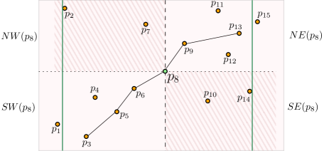
Figure 5: A collection of fifteen elements. Given a query range $q=[2,14]\times(-\infty,+\infty)$, suppose an oracle reveals that $p_{8}$ lies in the $\mathsf{LIS}$ of $\mathcal{P}\cap q$. Then observe that we can discard the points in $SE(p_{8})$ and $NW(p_{8})$ which are shown as shaded regions. The $\mathsf{LIS}$ of $\mathcal{P}\cap q\cap NE(p_{8})$ will be $(p_{8},p_{9},p_{13})$ and and the $\mathsf{LIS}$ of $\mathcal{P}\cap q\cap SW(p_{8})$ will be $(p_{3},p_{5},p_{6},p_{8})$. Therefore, $\mathsf{LIS}$ of $\mathcal{P}\cap q$ will be $(p_{3},p_{5},p_{6},p_{8},p_{9},p_{13})$.

Idea-2: Random sampling.

By using the fact that $\mathsf{LIS}(\mathcal{P}\cap q)\geq\tau$, it is possible to construct a set $\mathcal{R}$ of size roughly $\frac{n\log n}{\tau}\approx\sqrt{n}\log n$ via random sampling. For each $1\leq i\leq n$, sample $p_{i}\in\mathcal{P}$ independently with probability $\frac{c\log n}{\tau}$, where $c$ is a sufficiently large constant. Let $\mathcal{R}\subseteq\mathcal{P}$ be the set of sampled points. Then we can establish the following connection between $\mathcal{R}$ and the stitching elements.

Lemma 1.

For all ranges $q$ such that $\mathsf{LIS}(\mathcal{P}\cap q)\geq\tau$, if $S_{q}$ is one of the $\mathsf{LIS}$ of $\mathcal{P}\cap q$, then with high probability $|\mathcal{R}\cap S_{q}|=\Omega(\log n)$.

This ensures that the preprocessing time will be $O(|\mathcal{R}|n\log n)=O(n^{3/2}\log^{2}n)$. To answer any range $q$, first scan $\mathcal{R}$ to identify the points which lie inside $q$. For each element $p_{i}\in\mathcal{R}\cap q$, compute the right hand side of equation 1 in $O(\log n)$ time. Finally, report the largest value computed. Therefore, the query time is bounded by $O(|\mathcal{Q}|\cdot|\mathcal{R}|\cdot\log n)=O(m\sqrt{n}\log^{2}n)$.

1.4 Our third technique: Handling small cardinality colors

A naive approach.

The $\mathit{Colored\mbox{-}2D\mbox{-}Range\mbox{-}LIS}$ problem is more challenging than the $\mathit{2D\mbox{-}Range\mbox{-}LIS}$ problem. Firstly, the result of Theorem 2 does not really help in answering $\mathit{Colored\mbox{-}2D\mbox{-}Range\mbox{-}LIS}$ since it completely ignores the information about the colors. Secondly, there might be a temptation to solve the problem “independently” for each color class. For example, consider a setting where each color class has roughly equal number of points, i.e., $n/|\mathcal{C}|$ points. Consider a color $c$ and build an instance of Theorem 2 based on the points of color $c$. Then, for each query $q\in\mathcal{Q}$, we have the value of $\mathsf{LIS}(\mathcal{P}_{c}\cap q)$. Repeat this for each color in $\mathcal{C}$. Finally, for each query $q\in\mathcal{Q}$, report the color $c$ for which $\mathsf{LIS}(\mathcal{P}_{c}\cap q)$ is maximized.

Now lets (informally) analyze this algorithm. The running time bound of Theorem 2 has three terms. For now, lets ignore the second and the third term, which represent the time taken to build the data structure and the time taken to report the output of the $m$ queries. The first term is the time taken to answer $m$ queries (which is roughly $\sqrt{n}$ time per query). Adding the first term for each color class, we get

$$\sum_{c}\widetilde{O}(m|\mathcal{P}_{c}|^{1/2})\leq\widetilde{O}(|\mathcal{C}|m(n/|\mathcal{C}|)^{1/2})=\widetilde{O}(m\sqrt{n|\mathcal{C}|}),$$

which is $\widetilde{O}(mn)$ when $|\mathcal{C}|=\Theta(n)$ and $\widetilde{O}(mn^{\frac{1+\varepsilon}{2}})\gg m\sqrt{n}$ when $|\mathcal{C}|=n^{\varepsilon}$, for any $0<\varepsilon\leq 1$. Therefore, in the worst-case this approach does not help achieve our target query time bound.

A technique to handle small cardinality colors.

We will design a third technique which will be helpful to answer $\mathit{Colored\mbox{-}1D\mbox{-}Range\mbox{-}LIS}$ and $\mathit{Colored\mbox{-}2D\mbox{-}Range\mbox{-}LIS}$. The key idea is to handle all the colors in a “combined” manner. The technique will work well when all the colors have small cardinality. Given a parameter $\Delta$, assume that for each color $c$, the value of $|\mathcal{P}|_{c}\leq\Delta$. The key observations made by the algorithm are the following:

• Bounding the number of output subsequences. For a query $q$, let the output $\mathsf{LIS}$ be $S$ of color $c$. Let $p_{i}\in\mathcal{P}_{c}$ (resp., $p_{j}\in\mathcal{P}_{c}$) be the first (resp., last) point on $S$. Call this a pair $(i,j)$. As such, whenever color $c$ is the output, the number of distinct pairs will be $O(|\mathcal{P}_{c}|^{2})$. Adding up over all the colors, the total number of distinct pairs will be:

  $$\sum_{c}O(|\mathcal{P}_{c}|^{2})\leq O\left(\Delta\sum_{c}|\mathcal{P}_{c}|\right)=O(n\Delta).$$

  If $\Delta\ll n$, then this is a significant improvement over the naive bound of $O(n^{2})$ distinct pairs (or distinct output subsequences).

• Reduction to an uncolored problem. For each possible output subsequence $S$ of color $c$ with $p_{i}\in\mathcal{P}_{c}$ (resp., $p_{j}\in\mathcal{P}_{c}$) as the first (resp., last) point point on $S$, we construct an axis-aligned rectangle $R_{c}(i,j)$ with $p_{i}$ (resp., $p_{j}$) as the bottom-left (resp., top-right) corner. A weight $w(R_{c}(i,j))$ is associated with rectangle $R_{c}(i,j)$ which is equal to $\mathsf{LIS}(\mathcal{P}_{c}\cap R_{c}(i,j))$. See Figure 6. Let $\mathcal{R}$ be the collection of $O(n\Delta)$ such weighted rectangles. As a result, the problem of $\mathit{Colored\mbox{-}2D\mbox{-}Range\mbox{-}LIS}$ is now reduced to the rectangle range-max problem, where given an axis-parallel rectangle $q$, among all the rectangles in $\mathcal{R}$ which lie completely inside $q$, the goal is to report the rectangle with the largest weight.

  It is crucial to note that the colored problem has been reduced to a problem on uncolored rectangles for which an efficient data structure exists: the rectangle range-max data structure can be constructed in $\widetilde{O}(|\mathcal{R}|)=\widetilde{O}(n\Delta)$ time and the $m$ range queries can be answered in $\widetilde{O}(m)+O(k)$ time.

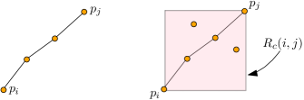
Figure 6: On the left is an increasing subsequence of length four with all four points being of color $c$. On the right is the corresponding rectangle $R_{c}(i,j)$. The $\mathsf{LIS}$ of color $c$ inside $R_{c}(i,j)$ is four (the other two points of color $c$ do not participate in the $\mathsf{LIS}$). Therefore, the weight associated with $R_{c}(i,j)$ is four.

1.5 Putting all the pieces together

As an illustration we will consider the $\mathit{Colored\mbox{-}2D\mbox{-}Range\mbox{-}LIS}$ problem and put together all the three techniques discussed in the previous subsections in a specific manner.

Light and heavy colors.

Define a parameter $\Delta$ which will be set later. A color $c$ is classified as light if $|\mathcal{P}_{c}|\leq\Delta$, otherwise, it is classified as heavy. We will design different algorithms to handle light colors and heavy colors. The advantage with a light color, say $c$, is that we can pre-compute the $\mathsf{LIS}$ for $O(|\mathcal{P}_{c}|^{2})$ 2D axis-parallel ranges and still be within the time budget. On the other hand, the advantage with heavy colors is that there can be only $O(n/\Delta)$ heavy colors.

Handling light colors.

Let $\mathcal{P}_{\ell}\subseteq\mathcal{P}$ be the set of points which belong to a light color. We will use the third technique to answer $\mathit{Colored\mbox{-}2D\mbox{-}Range\mbox{-}LIS}$ on $\mathcal{P}_{\ell}$ and queries $\mathcal{Q}$. From Section 4, it follows that the running time is $\widetilde{O}(m+n\Delta+k)$.

Handling heavy colors and small $\mathsf{LIS}$ queries.

Let $\mathcal{P}_{h}\subseteq\mathcal{P}$ be the set of points which belong to a heavy color. In Section 2, we will prove that for an arbitrary value of $\tau$, the running time of the first technique will be $\widetilde{O}(m\tau+n\tau)$. The first technique as described above only handles un-colored points. In Section 2, we will “generalize” the first technique to answer $\mathit{Colored\mbox{-}2D\mbox{-}Range\mbox{-}LIS}$ problem as well. The running time of this generalized first technique on colored pointset $\mathcal{P}_{h}$ and queries $\mathcal{Q}$ will be $\widetilde{O}\left(\frac{m\tau n}{\Delta}+\frac{n^{2}\tau}{\Delta}+k\right)$, where the number of heavy colors is $O(n/\Delta)$.

Handling heavy colors and large $\mathsf{LIS}$ queries.

In Section 3, we will prove that for an arbitrary $\tau$, the running time of the second technique will be $\widetilde{O}\left(\frac{mn}{\tau}+\frac{n^{2}}{\tau}+k\right)$ for $\mathit{2D\mbox{-}Range\mbox{-}LIS}$ problem. In fact, we will generalize this algorithm to the large $\mathsf{LIS}$ case of $\mathit{Colored\mbox{-}2D\mbox{-}Range\mbox{-}LIS}$ with the same running time (ignoring polylogarithmic factors). The generalized algorithm will answer $\mathit{Colored\mbox{-}2D\mbox{-}Range\mbox{-}LIS}$ on $\mathcal{P}_{h}$ and queries $\mathcal{Q}$.

Combining all the three subroutines, the total running time will be:

$$\widetilde{O}\underbrace{\left(m+\frac{mn}{\tau}+\frac{m\tau n}{\Delta}\right)}_{\text{query time}}+\underbrace{\widetilde{O}\left(\frac{n^{2}}{\tau}+n\Delta+\frac{n^{2}\tau}{\Delta}\right)}_{\text{preprocessing time}}+O\left(k\right)$$

We set the parameters $\tau\leftarrow n^{1/3}$ and $\Delta\leftarrow n^{2/3}$ in the above expression to obtain a running time of $\widetilde{O}(mn^{2/3}+n^{5/3}+k)$.

Organization of the paper.

The rest of the paper is organized as follows. In Section 2, we will discuss our first technique for handling queries in $\mathcal{Q}$ which have small $\mathsf{LIS}$. In Section 3, we will discuss our second technique for handling queries in $\mathcal{Q}$ which have large $\mathsf{LIS}$. In Section 4, we will discuss our final technique for handling colors in $\mathcal{P}$ which are light (cardinality is small). In Section 5, we will put all the techniques together in different ways to derive all the upper bounds. Next, in Section 6 we present our conditional lower bound. Finally, in Section 7, we present some open problems for future research.

2 First technique: Handling small $\mathsf{LIS}$

In this section, we describe a technique which efficiently handles queries with small $\mathsf{LIS}$. Consider a parameter $\tau\in[1,n]$ whose value will be set later.

2.1 2D Range $\mathsf{LIS}$ problem

We will illustrate the technique by first looking at the $\mathit{2D\mbox{-}Range\mbox{-}LIS}$ problem. The following result is obtained.

Theorem 6.

There is an algorithm for $\mathit{2D\mbox{-}Range\mbox{-}LIS}$ problem with running time $O(m\tau\log^{3}n+n\tau\log^{4}n+k)$, where $k$ is the cumulative length of all the output subsequences. For all queries $q\in\mathcal{Q}$ with $\mathsf{LIS}(\mathcal{P}\cap q)\leq\tau$, the algorithm returns the correct solution. For queries $q\in\mathcal{Q}$ with $\mathsf{LIS}(\mathcal{P}\cap q)>\tau$, correctness is not guaranteed.

The preprocessing phase of the algorithm consists of the following steps.

Lowest peaks and highest bases.

Consider the special case where there is a vertical line with $x$-coordinate $x^{*}$ such that each query range in $\mathcal{Q}$ intersects $x^{*}$. Let $\mathcal{P}_{\leq}\subseteq\mathcal{P}$ (resp., $\mathcal{P}_{>}\subseteq\mathcal{P}$) be the set of points with $x$-coordinate less than or equal to (resp., greater than) to $x^{*}$. For an increasing subsequence $S\in\mathcal{P}$, we define peak (resp., base) to be the last (resp., first) element in $S$. We will now define two arrays $A$ and $B$ as follows:

• For all $p_{i}\in\mathcal{P}_{\leq}$ and for all $1\leq\alpha\leq\tau$, among all increasing subsequences of length $\alpha$ in the range $[i,x^{*}]$ which have $p_{i}$ as the first element, let $S$ be the subsequence with the lowest peak. Then $A(p_{i},\alpha)$ stores the value of the last element in $S$.

• For all $p_{i}\in\mathcal{P}_{>}$ and for all $1\leq\beta\leq\tau$, among all increasing subsequences of length $\beta$ in the range $(x^{*},i]$ which have $p_{i}$ as the last element, let $S$ be the subsequence with the highest base. Then $B(p_{i},\beta)$ stores the value of the first element in $S$.

Efficient computation of $B$.

The next step is to compute each entry in $B$ in polylogarithmic time (analogous discussion holds for $A$). The entries will be computed in increasing values of $\beta$. Assume that the entries corresponding to sequences of length at most $\beta{-}1$ have been computed. Then the entries $B(p_{i},\beta)$’s can be reduced to entries of $B(\cdot,\beta-1)$’s as follows:

$$B(p_{i},\beta)=\begin{cases}a_{i},\quad\text{ if $\beta=1$;}\\ -\infty,\ \ \ \text{if $\beta>1$ and $a_{j}>a_{i}$ for all $\mathcal{P}_{>}\cap(x^{*},i)$;}\\ \max\{B(p_{j},\beta{-}1)\mid\ x^{*}<j<i\text{ and }a_{j}<a_{i}\},\quad\text{otherwise}.\end{cases}$$

We will reduce the problem of computing $B(p_{i},\beta)$ to the problem of constructing a data structure which can efficiently answer 2D range-max queries. In a 2D range-max problem, we are given $n$ weighted points $\mathcal{P}_{>}$ in 2D. Each point $p$ is associated with a weight. For each point $p_{i}=(i,a_{i})\in\mathcal{P}_{>}$, given a query region of the form $q^{\prime}=(-\infty,i)\times(-\infty,a_{i})$, the goal is to report the point in $\mathcal{P}_{>}\cap q^{\prime}$ with the maximum weight. The 2D range-max problem can be solved in $O(n\log n)$ time (via reduction to the so-called 2D orthogonal point location problem [ST86]).

Now with each point $p_{j}\in\mathcal{P}_{>}$, we associate weight $B(p_{j},\beta-1)$ and build a 2D range-max data structure. For each point $p_{i}=(i,a_{i})\in\mathcal{P}_{>}$, the point in $\mathcal{P}_{>}\cap((-\infty,i)\times(-\infty,a_{i}))$ with the maximum weight is reported. If point $p_{j}$ is reported, then set $B(p_{i},\beta)=B(p_{j},\beta-1)$. The correctness follows from the third case in the above dynamic programming. Since $\beta\leq\tau$, the time taken to construct $B$ is $O(\tau)\times O(n\log n)=O(n\tau\log n)$.

Data structures to compute $L$ and $R$.

During the query algorithm, we will need to compute some of the entries in two-dimensional arrays $L$ and $R$ which are defined as follows:

Array $L$:

For any $q\in\mathcal{Q}$ and for any $1\leq\alpha\leq\tau$, among all increasing subsequences of length $\alpha$ in $\mathcal{P}_{\leq}\cap q$, let $S$ be the subsequence with the lowest peak. Then $L(q,\alpha)$ is the value of the last element in $S$.

Array $R$:

For any $q\in\mathcal{Q}$ and for any $1\leq\beta\leq\tau$, among all increasing sequences of length $\beta$ in $\mathcal{P}_{>}\cap q$, let $S$ be the subsequence with the highest base. Then $R(q,\beta)$ is the value of the first element in $S$.

Each entry in $R$ is connected to entries in $B$ as follows:

$$R(q,\beta)\leftarrow\max_{p_{i}}\{B(p_{i},\beta)\mid p_{i}\in\mathcal{P}_{>}\cap q\text{ and }B(p_{i},\beta)>y_{1}\}.$$

Analogously, each entry in $L$ is connected to entries in $A$ as follows:

$$L(q,\alpha)\leftarrow\max_{p_{i}}\{A(p_{i},\alpha)\mid p_{i}\in\mathcal{P}_{\leq}\cap q\text{ and }A(p_{i},\alpha)<y_{2}\}.$$

Fix a value of $\beta$. We will now build a data structure to efficiently compute $R(q,\beta)$’s. For each point $p_{i}=(i,a_{i})\in\mathcal{P}_{>}$, map it to a point $p_{i}^{\prime}=(i,a_{i},B(p_{i},\beta))$ with weight $w(p_{i}^{\prime})\leftarrow B(p_{i},\beta)$. Let $\mathcal{P}_{>}^{\prime}$ be the collection of mapped 3D points. Build a 3D vanilla range tree [BCKO08] on $\mathcal{P}_{>}^{\prime}$. Given a query $q\in\mathcal{Q}$, it is transformed to a 3D cuboid $q^{\prime}=q\times(y_{1},+\infty)$ and the point with the maximum weight in $\mathcal{P}_{>}^{\prime}\cap q^{\prime}$ is reported efficiently. The time taken to construct the range tree is $O(n\log^{3}n)$. We will repeat this procedure for all values of $\beta\in[1,\tau]$. Therefore, the total construction time will be $O(n\tau\log^{3}n)$. Analogously, construct a data structure to efficiently compute $L(q,\alpha)$’s.

Recursion.

Let $\mathcal{D}$ be the data structure built above to handle queries in $\mathcal{Q}$ which intersect the vertical line with $x$-coordinate $x^{*}$. We will handle the general case via recursion. Let $x^{*}=n/2$, and let $\mathcal{P}_{\leq}\subseteq\mathcal{P}$ (resp., $\mathcal{P}_{>}\subseteq\mathcal{P}$) be the set of points with $x$-coordinate less than or equal to (resp., greater than) $x^{*}$. Recursively build data structure $\mathcal{D}_{\leq}$ (resp., $\mathcal{D}_{>}$) based on pointset $\mathcal{P}_{\leq}$ (resp., $\mathcal{P}_{>}$). The base case of $|\mathcal{P}|=1$ can be handled trivially. Let $T(n)$ be the total preprocessing time. Then,

$$T(n)\leq 2\cdot T(n/2)+O(n\tau\log^{3}n),$$

which solves to $T(n)=O(n\tau\log^{4}n)$.

Lemma 2.

The preprocessing time of the algorithm is $O(n\tau\log^{4}n)$.

Query algorithm.

The query algorithm consists of the following steps. Let $\mathcal{Q}_{x^{*}}\subseteq\mathcal{Q}$ be the set of queries which intersect the vertical line with $x$-coordinate $x^{*}=n/2$. We will first handle $\mathcal{Q}_{x^{*}}$. For each $q\in\mathcal{Q}_{x^{*}}$, compute $R(q,\beta)$, for all $1\leq\tau\leq\beta$, by querying the corresponding 3D range trees. Analogously, compute $L(q,\alpha)$ for all $1\leq\tau\leq\alpha$.

A pair $\left(L(q,\alpha),R(q,\beta)\right)$ is defined to be compatible if $L(q,\alpha)<R(q,\beta)$, i.e., it is possible to “stitch” the sequences corresponding to $L(q,\alpha)$ and $R(q,\beta)$ to obtain an increasing sequence of length $\alpha+\beta$. For a 2D query range $q$, our goal is to find the compatible pair $\left(L(q,\alpha),R(q,\beta)\right)$ which maximizes the value of $\alpha+\beta$, i.e.,

$$\mathsf{LIS}(\mathcal{P}\cap q)=\max_{\alpha,\beta}\{\alpha+\beta\mid L(q,\alpha)<R(q,\beta)\}.$$ (2)

To efficiently compute $\mathsf{LIS}(\mathcal{P}\cap q)$, we will use the monotonicity property of $R$: for a fixed query $q$, the value of $R(q,\beta)$ decreases as the value of $\beta$ increases, i.e., for any $1\leq\beta\leq\beta^{\prime}\leq\tau$, we have $R(q,\beta)\geq R(q,\beta^{\prime})$. For each $1\leq i\leq\tau$, the largest $\beta_{i}$ for which $(L(q,i),R(q,\beta_{i}))$ is compatible can be found in $O(\log\tau)$ time by doing a binary search on the monotone sequence $(R(q,1),R(q,2),\ldots,R(q,\tau))$. Finally, report $\max_{i}(i+\beta_{i})$ as the length of the $\mathsf{LIS}$ for $\mathcal{P}\cap q$. By appropriate bookkeeping, the corresponding $\mathsf{LIS}$ can be reported in time proportional to its length.

Let $\mathcal{Q}_{<}\subseteq\mathcal{Q}$ (resp., $\mathcal{Q}_{>}\subseteq\mathcal{Q}$) be the set of queries which lie completely to the left (resp., right) of the vertical line with $x$-coordinate $x^{*}$. Finally, recurse on pointset $\mathcal{P}_{\leq}$ and query set $\mathcal{Q}_{<}$, and recurse on pointset $\mathcal{P}_{>}$ and query set $\mathcal{Q}_{>}$.

Lemma 3.

The time taken answer the query ranges in $O(m\tau\log^{3}n+k)$.

Proof.

Fix a query range $q\in\mathcal{Q}$. Querying the 3D range trees takes $O(\log^{3}n)$ time. As such, the time taken to compute $R(q,\beta)$’s and $L(q,\alpha)$’s will be $O(\tau\log^{3}n)$. Next, computing the compatible pair which achieves the quantity $\max_{i}(i+\beta_{i})$ takes $O(\tau\log\tau)$ time. Therefore, the time spent per query is $O(\tau\log^{3}n+\tau\log\tau)=O(\tau\log^{3}n)$.

Assigning queries in $\mathcal{Q}$ to appropriate nodes in the recursion tree takes only $O(m\log n)$ time and is not the dominating term. ∎

2.2 Colored 2D Range $\mathsf{LIS}$ problem

The solution for $\mathit{Colored\mbox{-}2D\mbox{-}Range\mbox{-}LIS}$ is obtained by solving the $\mathit{2D\mbox{-}Range\mbox{-}LIS}$ problem independently for each color. Specifically, for each color $c\in\mathcal{C}$, solve the (uncolored) $\mathit{2D\mbox{-}Range\mbox{-}LIS}$ problem for $\mathcal{P}_{c}$ using Theorem 6. The length version of the $\mathit{2D\mbox{-}Range\mbox{-}LIS}$ problem will output for each $q\in\mathcal{Q}$ and each $c\in\mathcal{C}$, the value of $\mathsf{LIS}(\mathcal{P}_{c}\cap q)$. Then for each $q\in\mathcal{Q}$, report the color $c_{q}$ which maximizes the value of $\mathsf{LIS}(\mathcal{P}_{c_{q}}\cap q)$ and the corresponding $\mathsf{LIS}$. Ignoring the $k$ term, the running time of the algorithm is $|\mathcal{C}|$ times the running time of the $\mathit{2D\mbox{-}Range\mbox{-}LIS}$ problem.

Theorem 7.

There is an algorithm for $\mathit{Colored\mbox{-}2D\mbox{-}Range\mbox{-}LIS}$ problem with running time $O(m\tau|\mathcal{C}|\log^{3}n+n\tau|\mathcal{C}|\log^{4}n+k)$, where $k$ is the cumulative length of all the output subsequences. For all queries $q\in\mathcal{Q}$ with $\mathsf{LIS}(\mathcal{P}_{c_{q}}\cap q)\leq\tau$, the algorithm returns the correct solution. For queries $q\in\mathcal{Q}$ with $\mathsf{LIS}(\mathcal{P}_{c_{q}}\cap q)>\tau$, correctness is not guaranteed.

2.3 1D Range $\mathsf{LIS}$ problem

As discussed in Section 1.2, construction of arrays $A$ and $B$ takes $O(n\tau\log n)$ time. Also, in 1D the arrays $L$ and $R$ can be pre-computed and stored in the preprocessing phase. This takes only $O(n\tau)$ time. As such, the recurrence for the total preprocessing time will be:

$$T(n)\leq 2\cdot T(n/2)+O(n\tau\log n),$$

which solves to $T(n)=O(n\tau\log^{2}n)$.

Given a query range $q$, computing the compatible pair which achieves the quantity $\max_{i}(i+\beta_{i})$ takes $O(\tau\log\tau)=O(\tau\log n)$ time, and hence, the overall query time is $O(m\tau\log n)$.

Theorem 8.

There is an algorithm for $\mathit{1D\mbox{-}Range\mbox{-}LIS}$ problem with running time $O(m\tau\log n+n\tau\log^{2}n+k)$, where $k$ is the cumulative length of all the output subsequences. For all queries $q\in\mathcal{Q}$ with $\mathsf{LIS}(\mathcal{P}\cap q)\leq\tau$, the algorithm returns the correct solution. For queries $q\in\mathcal{Q}$ with $\mathsf{LIS}(\mathcal{P}\cap q)>\tau$, correctness is not guaranteed.

3 Second technique: Handling large $\mathsf{LIS}$

In this section, we describe a technique which efficiently handles queries with large $\mathsf{LIS}$. We will first consider the $\mathit{2D\mbox{-}Range\mbox{-}LIS}$ problem. Consider a parameter $\tau\in[1,n]$ whose value will be set later. The following result is obtained.

Theorem 9.

There is an algorithm for the $\mathit{2D\mbox{-}Range\mbox{-}LIS}$ problem with running time $O\left(\frac{mn}{\tau}\log^{5}n+\frac{n^{2}}{\tau}\log^{4}n+k\right)$, where $k$ is the cumulative length of all the output subsequences. The bound on the running time holds with high probability. For all queries $q\in\mathcal{Q}$ with $\mathsf{LIS}(\mathcal{P}\cap q)\geq\tau$, with high probability, the algorithm returns the correct solution.

Idea-1: Stitching elements.

Suppose an oracle reveals that point $p_{i}\in\mathcal{P}$ lies in the $\mathsf{LIS}$ of range $q=[x_{1},x_{2}]\times(-\infty,+\infty)$. Then we claim that the problem becomes decomposable. We will define some notation before proceeding. For a point $p_{i}=(i,a_{i})\in\mathcal{P}$ corresponding to an element $a_{i}\in\mathcal{S}$, define the north-east region of $p_{i}$ as $NE(p_{i})=\{(x,y)\mid x\geq i\text{ and }y\geq a_{i}\}$. Analogously, define the north-west, the south-west and the south-east region of $p_{i}$ which are denoted by $NW(p_{i}),SW(p_{i})\text{ and }SE(p_{i})$, respectively. Then it is easy to observe that,

$$\mathsf{LIS}(\mathcal{P}\cap q)=\mathsf{LIS}(\mathcal{P}\cap q\cap NE(p_{i}))+\mathsf{LIS}(\mathcal{P}\cap q\cap SW(p_{i}))-1.$$ (3)

See Figure 5 for an example. In other words, knowing that $p_{i}$ belongs to the $\mathsf{LIS}$ decomposes the original $\mathsf{LIS}$ problem into two $\mathsf{LIS}$ sub-problems which can be computed independently. In such a case, we refer to point $p_{i}$ as a stitching element, which is formally defined below.

Definition 2.

(Stitching element) For a range $q$, fix any $\mathsf{LIS}$ of $\mathcal{P}\cap q$ and call it $S$. Then each element in $S$ is defined to be a stitching element w.r.t. $q$.

The goal of our algorithm is to:

Construct a small-sized set $\mathcal{R}\subseteq\mathcal{P}$ such that, for any $q\in\mathcal{Q}$, at least one stitching element w.r.t. $q$ is contained in $\mathcal{R}\cap q$.

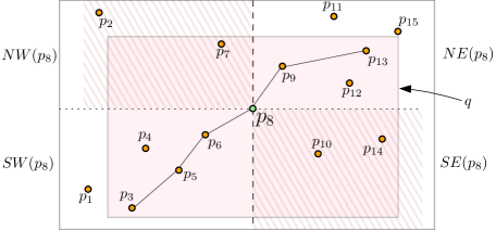
Figure 7: A collection of fifteen elements. Given a query range $q$ (shown in pink), suppose an oracle reveals that $p_{8}$ lies in the $\mathsf{LIS}$ of $\mathcal{P}\cap q$. Then observe that we can discard the points in $SE(p_{8})$ and $NW(p_{8})$ which are shown as shaded regions. The $\mathsf{LIS}$ of $\mathcal{P}\cap q\cap NE(p_{8})$ will be $(p_{8},p_{9},p_{13})$ and and the $\mathsf{LIS}$ of $\mathcal{P}\cap q\cap SW(p_{8})$ will be $(p_{3},p_{5},p_{6},p_{8})$. Therefore, $\mathsf{LIS}$ of $\mathcal{P}\cap q$ will be $(p_{3},p_{5},p_{6},p_{8},p_{9},p_{13})$.

Idea-2: Random sampling.

By using the fact that $\mathsf{LIS}(\mathcal{P}\cap q)\geq\tau$, it is possible to construct a set $\mathcal{R}$ of size $O\left(\frac{n\log n}{\tau}\right)$ via random sampling. For each $1\leq i\leq n$, sample $p_{i}\in\mathcal{P}$ independently with probability $\frac{c\log n}{\tau}$, where $c$ is a sufficiently large constant. Let $\mathcal{R}\subseteq\mathcal{P}$ be the set of sampled points. Then we can establish the following connection between $\mathcal{R}$ and the stitching elements.

Lemma 4.

For all ranges $q$ such that $\mathsf{LIS}(\mathcal{P}\cap q)\geq\tau$, if $S_{q}$ is one of the $\mathsf{LIS}$ of $\mathcal{P}\cap q$, then with high probability $|\mathcal{R}\cap S_{q}|=\Omega(\log n)$.

Proof.

Fix a range $q\in\mathcal{Q}$. For each point $e\in S_{q}$, let $X_{e}$ be an indicator random variable which is one if $e\in\mathcal{R}$, otherwise it is zero. Next, define another random variable $X=|\mathcal{R}\cap S_{q}|$. Then,

$${\bf E}[X]=\sum_{e\in S_{q}}{\bf E}[X_{e}]=|S_{q}|\cdot p\geq\tau\cdot\frac{c\log n}{\tau}=c\log n,$$

where we used the fact $|S_{q}|\geq\tau$. Next, for a sufficiently large constant $c^{\prime}$, we observe that

$${\bf Pr}\left(X<\frac{c\log n}{2}\right)\leq{\bf Pr}\left(X<\frac{{\bf E}[X]}{2}\right)\leq e^{-\frac{{\bf E}[X]}{8}}\leq\frac{1}{n^{c^{\prime}}},$$

where the second inequality follows by setting $\delta=1/2$ in the following version of Chernoff bound: ${\bf Pr}(X<(1-\delta){\bf E}[X])\leq e^{-\delta^{2}{\bf E}[X]/2}$, for $0<\delta<1$. Via a straightforward application of the union bound, with high probability none of the ranges $q\in\mathcal{Q}_{L}$ can have less than $\frac{c\log n}{2}$ elements in $\mathcal{R}\cap S_{q}$ (when $c\gg 16$). ∎

Computing restricted-$\mathsf{LIS}$’s efficiently.

For each query $q\in\mathcal{Q}$, if $p_{i}\in\mathcal{R}$ lies inside $q$, then we want to efficiently compute the quantities $\mathsf{LIS}(\mathcal{P}\cap q\cap NE(p_{i}))$ and $\mathsf{LIS}(\mathcal{P}\cap q\cap SW(p_{i}))$ (as shown in equation 3). To enable that, we will now compute restricted-$\mathsf{LIS}$’s between some specifically chosen pairs of points.

Consider a point $p_{i}=(i,a_{i})\in\mathcal{R}$. Scan the points $\mathcal{P}\cap NE(p_{i})$ in increasing order of their $x$-coordinate value. We will assign a weight $w(p_{j})$ for each point encountered. As a base case, we will assign $w(p_{i})\leftarrow 1$. At a general step, if we encounter point $p_{j}$, then we

$$w(p_{j})\leftarrow 1+\max_{p_{\alpha}=(\alpha,a_{\alpha})\in(\mathcal{P}\cap NE(p_{i}))}\{w(p_{\alpha})\mid\alpha<j\text{ and }a_{\alpha}<a_{j}\}.$$ (4)

See Figure 8 for an example. Repeat this process for each point in $\mathcal{R}$. Now we claim the following.

Lemma 5.

For a given query $q\in\mathcal{Q}$, let $p_{i}\in\mathcal{R}\cap q$. Then $\mathsf{LIS}(\mathcal{P}\cap q\cap NE(p_{i}))\leftarrow\max_{p_{j}\in(\mathcal{P}\cap q\cap NE(p_{i}))}\{w(p_{j})\}$.

Proof.

The correctness follows from the fact that $w(p_{j})$ captures the length of the $\mathsf{LIS}$ which has $p_{i}$ (resp., $p_{j}$) as the first (resp., last) point. ∎

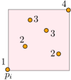
Figure 8: $p_{i}$ is a point in $\mathcal{R}$ and $NE(p_{i})$ has six points. The weight computed for each point by Equation 4 is shown besides each point.

Lemma 6.

The computation of restricted-$\mathsf{LIS}$’s, i.e., computation of $w(p_{j})$, for all $p_{j}\in\mathcal{P}\cap NE(p_{i})$ can be done in $O(n\log^{2}n)$ time.

Proof.

Construct a vanilla range-tree [BCKO08] based on the points $\mathcal{P}\cap NE(p_{i})$. Set the weight of $p_{i}$ equal to one and the weight of remaining points to $-\infty$. Whenever a point $p_{j}$ is encountered, then query the range tree with query rectangle $q^{\prime}=(-\infty,j)\times(-\infty,a_{j})$ and report the point in $\mathcal{P}\cap NE(p_{i})\cap q^{\prime}$ with the maximum weight. The query time is $O(\log^{2}n)$. If $p_{\alpha}$ is the point reported, update the range tree with the new weight of $w(p_{j})\leftarrow 1+w(p_{\alpha})$. The update takes $O(\log^{2}n)$ amortized time. ∎

Lemma 7.

There is an algorithm, which with high probability, computes restricted-$\mathsf{LIS}$’s for all points in $\mathcal{R}$ in $O\left(\frac{n^{2}}{\tau}\log^{3}n\right)$ time.

Proof.

For all $1\leq i\leq n$, let $X_{i}$ be the random variable which is one if $p_{i}\in\mathcal{R}$, otherwise it is zero. Let $T$ be the random variable which is the time taken to compute restricted-$\mathsf{LIS}$’s, for all points in $\mathcal{R}$. Then, by Lemma 6, we have

$$T=O(n\log^{2}n)\cdot\sum_{i=1}^{n}X_{i}+O(n).$$

Now consider the random variable $X$ which is equal to $\sum_{i=1}^{n}X_{i}$. Then ${\bf E}[X]={\bf E}[\sum_{i=1}^{n}X_{i}]=\frac{cn}{\tau}\log n$. Let $c^{\prime}$ be a sufficiently large constant. By using an appropriate version of Chernoff bound, we observe that

$${\bf Pr}\left(X>\frac{2cn}{\tau}\log n\right)\leq{\bf Pr}(X>2{\bf E}[X])<e^{-\Omega({\bf E}[X])}<\frac{1}{n^{c^{\prime}}},$$

where the last inequality used the trivial fact that ${\bf E}[X]\geq c\log n$. Therefore, with high probability $T$ is bounded by $O\left(\frac{n^{2}}{\tau}\log^{3}n\right)$. ∎

We will perform an analogous procedure for computing $\mathsf{LIS}(\mathcal{P}\cap q\cap SW(p_{i}))$, for each $p_{i}\in\mathcal{R}$.

Representing restricted-$\mathsf{LIS}$s as rectangles.

Consider a point $p_{i}\in\mathcal{R}$. For each point $p_{j}\in\mathcal{P}\cap NE(p_{i})$, let $B_{ij}$ be an axis-parallel rectangle with $p_{i}$ as the lower-left corner and $p_{j}$ as the top-right corner, with an associated weight of $w(p_{j})$. Let $\mathcal{B}_{i}$ the collection of these rectangles. Define $\mathcal{B}\leftarrow\bigcup_{p_{i}\in\mathcal{P}}\mathcal{B}_{i}$.

In a rectangle range-max query, the input is a set $\mathcal{B}$ of weighted axis-aligned rectangles in 2D. Given a query rectangle $q$, among all the rectangles in $\mathcal{B}$ which lie completely inside $q$, the goal is to report the rectangle with the largest weight. We will use (vanilla) 4D range trees as our data structure [BCKO08]. The data structure can be constructed in $O(|\mathcal{B}|\log^{3}|\mathcal{B}|)=O\left(\frac{n^{2}}{\tau}\log^{4}n\right)$ time and the rectangle range-max query can be answered in $O(\log^{4}|\mathcal{B}|)=O(\log^{4}n)$ time. The bounds hold with high probability.

Lemma 8.

The preprocessing time of the algorithm is $O\left(\frac{n^{2}}{\tau}\log^{4}n\right)$. The bound holds with high probability.

Proof.

By Lemma 7, construction of all the restricted-$\mathsf{LIS}$’s takes $O\left(\frac{n^{2}}{\tau}\log^{3}n\right)$ time. The preprocessing time is dominated by the construction time of set $\mathcal{B}$ which is $O\left(\frac{n^{2}}{\tau}\log^{4}n\right)$. ∎

The following lemma establishes the connection between Lemma 5 and set $\mathcal{B}$.

Lemma 9.

For a given query $q\in\mathcal{Q}$, let $p_{i}\in\mathcal{R}\cap q$. Then $\mathsf{LIS}(\mathcal{P}\cap q\cap NE(p_{i}))$ is equal to the weight of the largest weighted rectangle in $\mathcal{B}$ which lies completely inside $q\cap NE(p_{i})$.

Query algorithm.

Consider any range $q\in\mathcal{Q}$. Scan $\mathcal{R}$ to identify the points which lie inside $q$. If $|\mathcal{R}\cap q|=\emptyset$, then we do not proceed further for $q$. Otherwise, for each element $p_{i}\in\mathcal{R}\cap q$, we want to compute

$$\mathsf{LIS}(\mathcal{P}\cap q\cap NE(p_{i}))+\mathsf{LIS}(\mathcal{P}\cap q\cap SW(p_{i}))-1.$$

To compute $\mathsf{LIS}(\mathcal{P}\cap q\cap NE(p_{i}))$, we use Lemma 9 and pose a rectangle range-max query on $\mathcal{B}$ with query $q\cap NE(p_{i})$. Analogously, we compute $\mathsf{LIS}(\mathcal{P}\cap q\cap SW(p_{i}))$. Finally, report the largest value computed. By Lemma 4, we claim that the answer is correct with high probability if $\mathsf{LIS}(\mathcal{P}\cap q)\geq\tau$. Repeat this procedure for each $q\in\mathcal{Q}$. The query time will be $O(|\mathcal{Q}||\mathcal{R}|\log^{4}n)$ which will be $O\left(\frac{mn}{\tau}\log^{5}n\right)$ with high probability. By appropriate bookkeeping, reporting the $\mathsf{LIS}$ of $\mathcal{P}\cap q$, for all $q\in\mathcal{Q}$ can be done in $O(k)$ time.

Lemma 10.

The query time of the algorithm is $O\left(\frac{mn}{\tau}\log^{5}n+k\right)$. With high probability, the correctness and the bound on the running time holds.

This finishes the proof of Theorem 9.

3.1 Adapting the technique to other problems

Colored 2D range $\mathsf{LIS}$.

In the $\mathit{Colored\mbox{-}2D\mbox{-}Range\mbox{-}LIS}$ problem, for each $q\in\mathcal{Q}$, let $c_{q}\in\mathcal{C}$ be the color for which $\mathsf{LIS}(\mathcal{P}_{c_{q}}\cap q)$ is maximized. The algorithm for $\mathit{Colored\mbox{-}2D\mbox{-}Range\mbox{-}LIS}$ requires two modifications to the algorithm for $\mathit{2D\mbox{-}Range\mbox{-}LIS}$. The first modification is the precise connection between $\mathcal{R}$ and the stitching elements.

Lemma 11.

For all ranges $q$ such that $\mathsf{LIS}(\mathcal{P}_{c_{q}}\cap q)\geq\tau$, if $S_{q}$ is one of the $\mathsf{LIS}$ of $\mathcal{P}_{c_{q}}\cap q$, then with high probability $|\mathcal{R}\cap S_{q}|=\Omega(\log n)$.

Let $p_{i}\in\mathcal{R}$ have color $c$. Next, we modify Equation 4 by replacing $\mathcal{P}$ with $\mathcal{P}_{c}$. Specifically, we do the following:

$$w(p_{j})\leftarrow 1+\max_{p_{\alpha}=(\alpha,a_{\alpha})\in(\mathcal{P}_{c}\cap NE(p_{i}))}\{w(p_{\alpha})\mid\alpha<j\text{ and }a_{\alpha}<a_{j}\}.$$ (5)

The remaining preprocessing steps and the query algorithm of $\mathit{2D\mbox{-}Range\mbox{-}LIS}$ can be trivially adapted for the $\mathit{Colored\mbox{-}2D\mbox{-}Range\mbox{-}LIS}$ problem. The final result is summarized below.

Theorem 10.

There is an algorithm for the $\mathit{Colored\mbox{-}2D\mbox{-}Range\mbox{-}LIS}$ problem with running time $O\left(\frac{mn}{\tau}\log^{5}n+\frac{n^{2}}{\tau}\log^{4}n+k\right)$, where $k$ is the cumulative length of all the output subsequences. The bound on the running time holds with high probability. For all queries $q\in\mathcal{Q}$ with $\mathsf{LIS}(\mathcal{P}_{c_{q}}\cap q)\geq\tau$, with high probability, the algorithm returns the correct solution.

Shaving log factors in 1D.

To answer $\mathit{1D\mbox{-}Range\mbox{-}LIS}$ and $\mathit{Colored\mbox{-}1D\mbox{-}Range\mbox{-}LIS}$, the rectangle range-max data structure can be replaced by interval range-max data structure. For each rectangle $B\in\mathcal{B}$, let $I$ be the projection of $B$ onto the $x$-axis. The weight of $I$ is equal to the weight of $B$, for all $B\in\mathcal{B}$. Let $\mathcal{I}\leftarrow\bigcup_{B\in\mathcal{B}}I$ be the collection of weighted intervals. In an interval range-max query, the input is a set $\mathcal{I}$ of weighted intervals on the real line. Given a query range $q$, among all the intervals in $\mathcal{I}$ which lie completely inside $q$, the goal is to report the interval with the largest weight.

The interval range max data structure can be constructed in $O(|\mathcal{I}|\log|\mathcal{I}|)=O\left(\frac{n^{2}}{\tau}\log^{2}n\right)$ time (via reduction to 2D orthogonal point location problem [ST86]) and the query can be answered in $O(\log|\mathcal{I}|)=O(\log n)$ time. Therefore, in 1D the preprocessing time reduces from $O\left(\frac{n^{2}}{\tau}\log^{4}n\right)$ to $O\left(\frac{n^{2}}{\tau}\log^{3}n\right)$, and the query time reduces from $O\left(\frac{mn}{\tau}\log^{5}n\right)$ to $O\left(\frac{mn}{\tau}\log^{2}n\right)$. We summarize the 1D results below.

Theorem 11.

There is an algorithm for the $\mathit{Colored\mbox{-}1D\mbox{-}Range\mbox{-}LIS}$ problem with running time $O\left(\frac{mn}{\tau}\log^{2}n+\frac{n^{2}}{\tau}\log^{3}n+k\right)$, where $k$ is the cumulative length of all the output subsequences. The bound on the running time holds with high probability. For all queries $q\in\mathcal{Q}$ with $\mathsf{LIS}(\mathcal{P}_{c_{q}}\cap q)\geq\tau$, with high probability, the algorithm returns the correct solution.

Theorem 12.

There is an algorithm for the $\mathit{1D\mbox{-}Range\mbox{-}LIS}$ problem with running time $O\left(\frac{mn}{\tau}\log^{2}n+\frac{n^{2}}{\tau}\log^{3}n+k\right)$, where $k$ is the cumulative length of all the output subsequences. The bound on the running time holds with high probability. For all queries $q\in\mathcal{Q}$ with $\mathsf{LIS}(\mathcal{P}\cap q)\geq\tau$, with high probability, the algorithm returns the correct solution.

4 Third technique: Handling small cardinality colors

In this section we will discuss a technique to handle colored $\mathit{Range\mbox{-}LIS}$ problems. The algorithm is efficient when each color class has a small cardinality. We will prove the following two results.

Theorem 13.

Fix a parameter $\Delta$. Then there is a deterministic algorithm to answer $\mathit{Colored\mbox{-}2D\mbox{-}Range\mbox{-}LIS}$ problem in $O(m\log^{4}n+n\Delta\log^{4}n+k)$ time, where for each color $c\in\mathcal{C}$, we have $|\mathcal{P}_{c}|\leq\Delta$, and $k$ is the cumulative length of the $m$ output subsequences.

Theorem 14.

Fix a parameter $\Delta$. Then there is a deterministic algorithm to answer $\mathit{Colored\mbox{-}1D\mbox{-}Range\mbox{-}LIS}$ problem in $O(m\log n+n\Delta\log^{2}n+k)$ time, where for each color $c\in\mathcal{C}$, we have $|\mathcal{P}_{c}|\leq\Delta$, and $k$ is the cumulative length of the $m$ output subsequences.

We will first consider the $\mathit{Colored\mbox{-}2D\mbox{-}Range\mbox{-}LIS}$ problem. For a query $q$, let the output $\mathsf{LIS}$ be $S$ of color $c$. Let $p_{i}\in\mathcal{P}_{c}$ (resp., $p_{j}\in\mathcal{P}_{c}$) be the first (resp., last) point on $S$. Call this a pair $(i,j)$. As such, whenever color $c$ is the output, the number of distinct pairs will be $O(|\mathcal{P}_{c}|^{2})$. Adding up over all the colors, the total number of distinct pairs will be:

$$\sum_{c}O(|\mathcal{P}_{c}|^{2})\leq O\left(\Delta\sum_{c}|\mathcal{P}_{c}|\right)=O(n\Delta).$$

We will pre-compute and store the length of the $\mathsf{LIS}$ corresponding to each pair $(i,j)$. See Figure 6 for an example.

Constructing the set $\mathcal{R}$.

Consider a color $c$ and a point $p_{i}=(i,a_{i})\in\mathcal{P}_{c}$. Define $NE(p_{i})$ to be set of points in 2D which lie in the north-east region of $p_{i}$, i.e., $NE(p_{i})=\{(p_{x},p_{y})\mid p_{x}>i\text{ and }p_{y}>a_{i}\}$. Consider the points $\mathcal{P}_{c}\cap NE(p_{i})$ in increasing order of their $x$-coordinate value. We will assign a weight $w(p_{j})$ for each point encountered. As a base case, we will assign $w(p_{i})\leftarrow 1$. At a general step, if we encounter point $p_{j}$, then we

$$w(p_{j})\leftarrow 1+\max_{p_{\alpha}=(\alpha,a_{\alpha})\in(\mathcal{P}_{c}\cap NE(p_{i}))}\{w(p_{\alpha})\mid\alpha<j\text{ and }a_{\alpha}<a_{j}\}.$$ (6)

See Figure 9 where $p_{j}$ is assigned a weight of four. Construct an axis-aligned rectangle $R_{c}(i,j)$ with $p_{i}$ (resp., $p_{j}$) as the bottom-left (resp., top-right) corner. A weight of $w(p_{j})$ is associated with $R_{c}(i,j)$. The intuition is that $w(p_{j})$ is equal to the $\mathsf{LIS}$ of the points of color $c$ lying inside $R_{c}(i,j)$, i.e., $\mathsf{LIS}(\mathcal{P}_{c}\cap R_{c}(i,j))$.

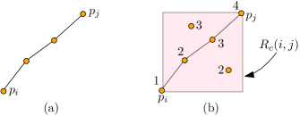
Figure 9: (a) An increasing subsequence of length four with all four points being of color $c$. (b) The weight computed by Equation 6 is shown besides each point. The $\mathsf{LIS}$ of color $c$ inside $R_{c}(i,j)$ is four (the other two points of color $c$ do not participate in the $\mathsf{LIS}$). Therefore, the weight associated with $R_{c}(i,j)$ is four.

The computation of $w(p_{j})$, for all $p_{j}\in\mathcal{P}_{c}\cap NE(p_{i})$ can be done in $O(|\mathcal{P}_{c}|\log^{2}|\mathcal{P}_{c}|)$ time. Construct a vanilla range-tree [BCKO08] based on the points $\mathcal{P}_{c}\cap NE(p_{i})$. Set the weight of $p_{i}$ equal to one and the weight of remaining points to $-\infty$. Whenever a point $p_{j}$ is encountered, then query the range tree with query rectangle $q^{\prime}=(-\infty,j)\times(-\infty,a_{j})$ and report the point in $\mathcal{P}_{c}\cap NE(p_{i})\cap q^{\prime}$ with the maximum weight. The query time is $O(\log^{2}|\mathcal{P}_{c}|)$. If $p_{\alpha}$ is the point reported, update the range tree with the new weight of $w(p_{j})\leftarrow 1+w(p_{\alpha})$. The update takes $O(\log^{2}|\mathcal{P}_{c}|)$ amortized time.

Repeat this procedure for each point in $\mathcal{P}_{c}$. This takes $O(|\mathcal{P}_{c}|^{2}\log^{2}|\mathcal{P}_{c}|)$ time. Define $\mathcal{R}_{c}\leftarrow\bigcup_{(i,j)}R_{c}(i,j)$ and $\mathcal{R}\leftarrow\bigcup_{c}\mathcal{R}_{c}$ which is a collection of rectangles corresponding to the distinct pairs $(i,j)$. The total time taken to construct $\mathcal{R}$ will be $\sum_{c}O(|\mathcal{P}_{c}|^{2}\log^{2}|\mathcal{P}_{c}|)=O(n\Delta\log^{2}n)$.

Rectangle range-max structure.

In a rectangle range-max query, the input is a set $\mathcal{R}$ of weighted axis-aligned rectangles in 2D. Given a query rectangle $q$, among all the rectangles in $\mathcal{R}$ which lie completely inside $q$, the goal is to report the rectangle with the largest weight. Note that in the rectangle range-max query, the color of the rectangles does not matter. We are dealing with uncolored rectangles and as a result, we can use vanilla 4D range trees as our data structure [BCKO08]. The data structure can be constructed in $O(|\mathcal{R}|\log^{4}|\mathcal{R}|)=O(n\Delta\log^{4}n)$ time and the rectangle range-max query can be answered in $O(\log^{4}|\mathcal{R}|)=O(\log^{4}n)$ time.

Coming back to our $\mathit{Colored\mbox{-}2D\mbox{-}Range\mbox{-}LIS}$ problem, for a query range $q\in\mathcal{Q}$, we first query the rectangle range-max data structure. Let $c_{q}$ be the color corresponding to the reported rectangle. We claim that $c_{q}$ is the color for which $\mathsf{LIS}(\mathcal{P}_{c_{q}}\cap q)$ is maximized. Overall, answering $m$ range queries in $\mathcal{Q}$ requires only $O(m\log^{4}n)$ time. By appropriate bookkeeping, reporting the $\mathsf{LIS}$ of $\mathcal{P}_{c_{q}}\cap q$, for all $q\in\mathcal{Q}$ can be done in $O(k)$ time. This finishes the proof of Theorem 13.

Shaving log factors in 1D.

To answer $\mathit{Colored\mbox{-}1D\mbox{-}Range\mbox{-}LIS}$ the rectangle range-max data structure can be replaced by interval range-max data structure. For each rectangle $R\in\mathcal{R}$, let $I$ be the projection of $R$ onto the $x$-axis. The weight of $I$ is equal to the weight of $R$, for all $R\in\mathcal{R}$. Let $\mathcal{I}\leftarrow\bigcup_{R\in\mathcal{R}}I$ be the collection of weighted intervals. In an interval range-max query, the input is a set $\mathcal{I}$ of weighted intervals on the real line. Given a query range $q$, among all the intervals in $\mathcal{I}$ which lie completely inside $q$, the goal is to report the interval with the largest weight.

The interval range max data structure can be constructed in $O(|\mathcal{I}|\log|\mathcal{I}|)=O(n\Delta\log n)$ time (via reduction to 2D orthogonal point location problem [ST86]) and the query can be answered in $O(\log|\mathcal{I}|)=O(\log n)$ time. This finishes the proof of Theorem 14.

5 Putting all the techniques together

Finally, in this section we will put together all the three techniques to obtain our upper bound results.

5.1 1D Range $LIS$ problem

The algorithm for $\mathit{1D\mbox{-}Range\mbox{-}LIS}$ applies the first technique on $\mathcal{P}$ and $\mathcal{Q}$, and then applies the second technique on $\mathcal{P}$ and $\mathcal{Q}$. For each query $q\in\mathcal{Q}$, with high probability, the correct solution is returned by one of them. Using Theorem 8, the running time of the first technique is $O(m\tau\log n+n\tau\log^{2}n+k)$. Using Theorem 12, the running time of the second technique is $O\left(\frac{mn}{\tau}\log^{2}n+\frac{n^{2}}{\tau}\log^{3}n+k\right)$. Setting $\tau\leftarrow\sqrt{n}$, we obtain a total running time of $O(m\sqrt{n}\log^{2}n+n\sqrt{n}\log^{3}+k)$. This proves Theorem 1.

5.2 2D Range $\mathsf{LIS}$ problem

The algorithm for $\mathit{2D\mbox{-}Range\mbox{-}LIS}$ applies the first technique on $\mathcal{P}$ and $\mathcal{Q}$, and then applies the second technique on $\mathcal{P}$ and $\mathcal{Q}$. For each query $q\in\mathcal{Q}$, with high probability, the correct solution is returned by one of them. Using Theorem 6, the running time of the first technique is $O(m\tau\log^{3}n+n\tau\log^{4}n+k)$. Using Theorem 9, the running time of the second technique is $O\left(\frac{mn}{\tau}\log^{5}n+\frac{n^{2}}{\tau}\log^{4}n+k\right)$. Setting $\tau\leftarrow\sqrt{n}$, we obtain a total running time of $O(m\sqrt{n}\log^{5}n+n\sqrt{n}\log^{4}+k)$. This proves Theorem 2.

5.3 Colored 1D range $\mathsf{LIS}$ problem

The algorithm consists of the following steps.

Light and heavy colors.

Define a parameter $\Delta$ which is set to $\sqrt{n}$. A color $c$ is classified as light if $|\mathcal{P}_{c}|\leq\Delta$, otherwise, it is classified as heavy. We will design different algorithms to handle light colors and heavy colors.

Querying light colors simultaneously.

Let $\mathcal{P}_{\ell}\subseteq\mathcal{P}$ be the set of points having light color. We will use the third technique to answer $\mathit{Colored\mbox{-}1D\mbox{-}Range\mbox{-}LIS}$ on $\mathcal{P}_{\ell}$. By Theorem 14, the running time is $O(m\log n+n\sqrt{n}\log^{2}n+k)$.

Query heavy colors independently.

For each heavy color, we build Tiskin’s structure and the structure of Theorem 1 to answer the length version and the reporting version of $\mathit{1D\mbox{-}Range\mbox{-}LIS}$, respectively. Given a query $q\in\mathcal{Q}$, we query the length structure of each heavy color and find the color $c_{q}$ for which $\mathsf{LIS}(\mathcal{P}_{c_{q}}\cap q)$ is maximized. Finally, query the reporting structure of color $c_{q}$ to report the $\mathsf{LIS}$ of $\mathcal{P}_{c_{q}}\cap q$.

The preprocessing time (dominated by the construction of reporting structures) is $O(n\sqrt{n}\log^{3}n)$ (Theorem 1). Since the number of heavy colors is $O(\sqrt{n})$, querying the length structure takes $O(\sqrt{n}\log n)$ time per query, and querying the reporting structure takes $O(\sqrt{n}\log^{2}n+k_{q})$ time per query, where $k_{q}$ is the length of the $\mathsf{LIS}$ reported. As such, the time taken to answer all the $m$ queries will be $O(m\sqrt{n}\log^{2}n+k)$.

Overall algorithm.

For each query $q\in\mathcal{Q}$, after querying the light colors and the heavy colors, report the larger among the two sequences reported. The overall running time of the algorithm is $O(m\sqrt{n}\log^{2}n+n\sqrt{n}\log^{3}n+k)$. This proves Theorem 3.

5.4 Colored 2D range $\mathsf{LIS}$ problem

The algorithm for $\mathit{Colored\mbox{-}2D\mbox{-}Range\mbox{-}LIS}$ is slightly more nuanced than $\mathit{Colored\mbox{-}1D\mbox{-}Range\mbox{-}LIS}$.

Light and heavy colors.

Define a parameter $\Delta$ which will be set later. A color $c$ is classified as light if $|\mathcal{P}_{c}|\leq\Delta$, otherwise, it is classified as heavy. We will design different algorithms to handle light colors and heavy colors. The advantage with a light color, say $c$, is that we can pre-compute the $\mathsf{LIS}$ for $O(|\mathcal{P}_{c}|^{2})$ 2D axis-parallel ranges and still be within the time budget. On the other hand, the advantage with heavy colors is that there can be only $O(n/\Delta)$ heavy colors.

Handling light colors.

Let $\mathcal{P}_{\ell}\subseteq\mathcal{P}$ be the set of points which belong to a light color. We will use the third technique on $\mathcal{P}_{\ell}$ and queries $\mathcal{Q}$. Using Theorem 13, it follows that the running time is $O(m\log^{4}n+n\Delta\log^{4}n+k)$.

Handling heavy colors and small $\mathsf{LIS}$ queries.

Let $\mathcal{P}_{h}\subseteq\mathcal{P}$ be the set of points which belong to a heavy color. We will use the first technique in Section 2 on $\mathcal{P}_{h}$ and queries $\mathcal{Q}$. The running time is $O\left(\frac{m\tau n}{\Delta}\log^{3}n+\frac{n^{2}\tau}{\Delta}\log^{4}n+k\right)$.

Handling heavy colors and large $\mathsf{LIS}$ queries.

We will use the second technique in Section 3 on $\mathcal{P}_{h}$ and queries $\mathcal{Q}$. The running time is $O\left(\frac{mn}{\tau}\log^{5}n+\frac{n^{2}}{\tau}\log^{4}n+k\right)$.

Overall algorithm.

For each query $q\in\mathcal{Q}$, after querying each of the above three subroutines, report the largest among the three sequences reported. Combining all the three subroutines, the total running time will be:

$$\underbrace{O\left(m\log^{4}n+\frac{mn}{\tau}\log^{5}n+\frac{m\tau n}{\Delta}\log^{3}n\right)}_{\text{query time}}+\underbrace{O\left(\frac{n^{2}}{\tau}\log^{4}n+n\Delta\log^{4}n+\frac{n^{2}\tau}{\Delta}\log^{4}n\right)}_{\text{preprocessing time}}+O\left(k\right)$$

We set the parameters $\tau\leftarrow n^{1/3}$ and $\Delta\leftarrow n^{2/3}$ in the above expression to obtain a running time of $O(mn^{2/3}\log^{5}n+n^{5/3}\log^{4}n+k)$. This proves Theorem 5.

6 Conditional Lower Bound

In this section we prove Theorem 4. Before we do so, we first recall the Combinatorial Boolean Matrix Multiplication Hypothesis ($\mathsf{CBMMH}$) and a conditional lower bound of [CDL⁺14] on computing mode for range queries.

Definition 3 (Combinatorial Boolean Matrix Multiplication conjecture).

The Combinatorial Boolean Matrix Multiplication conjecture asserts that for every $\varepsilon>0$, no combinatorial algorithm running in time $n^{1.5-\varepsilon}$ can given as input two $\sqrt{n}\times\sqrt{n}$ Boolean matrices, compute their product.

Computing Mode for Range Queries.

A mode of a multiset $S$ is an element $a\in S$ of maximum multiplicity; that is, $a$ occurs at least as frequently as any other element in $S$. Given a sequence $\mathcal{T}$ of $n$ elements and set of $m$ range queries $\mathcal{Q}$, for each query $q\in\mathcal{Q}$, the goal is to answer the mode of $\mathcal{T}\cap q$.

Theorem 15 (Chan et al. [CDL⁺14]).

Suppose there is an algorithm that takes as input a sequence of $n$ elements and set of $m$ range queries, runs in time $O(n^{c}\cdot(m+n))$ (for some $c\geq 0)$, and outputs the mode for all range queries, then Boolean matrix multiplication on two $\sqrt{n}\times\sqrt{n}$ matrices can be solved in time $O(n^{1+c})$.

We are now ready to prove Theorem 4.

Proof of Theorem 4.

Suppose there is some $\varepsilon>0$, and a combinatorial algorithm $\widetilde{\mathcal{A}}$ to answer the reporting version of the $\mathit{Colored\mbox{-}1D\mbox{-}Range\mbox{-}LIS}$ problem in $O(n^{1/2-\varepsilon}\cdot(m+n))$ time. Then, we construct an algorithm to refute $\mathsf{CBMMH}$ in the following way.

Given as input a sequence $\mathcal{T}:=(z_{1},\ldots,z_{n})$ of $n$ elements and set of $m$ mode range queries $\mathcal{Q}$, we construct an instance $(\mathcal{S}:=(a_{1},\ldots,a_{n}),c:\mathcal{S}\to[n],\mathcal{Q})$ of $\mathit{Colored\mbox{-}1D\mbox{-}Range\mbox{-}LIS}$ as follows. Without loss of generality, we assume all elements in $\mathcal{T}$ are in $[n]$. For every $i\in[n]$, let $f_{i}$ be the number of times the $z_{i}$ has appeared in $\mathcal{T}$ at an index less than $i$. Then, we define $a_{i}:=z_{i}+(f_{i}\cdot n)$. Note that we can compute $\mathcal{S}$ from $\mathcal{T}$ in $O(n\log n)$ time. Moreover, we define the color of $a_{i}$, i.e., $c(a_{i})$ to simply be $z_{i}$.

We will now use $\widetilde{\mathcal{A}}$ to answer the mode range queries in $\mathcal{Q}$ in $O(n^{1/2-\varepsilon}\cdot(m+n)+n\log n)$ time as follows (and this would contradict $\mathsf{CBMMH}$ from Theorem 15).

We feed $(\mathcal{S},c,\mathcal{Q})$ to $\widetilde{\mathcal{A}}$ and obtain in $O(n^{1/2-\varepsilon}\cdot(m+n))$ time, for every $q\in\mathcal{Q}$, the longest monochromatic increase subsequence $\mathcal{S}_{q}$ in $\mathcal{S}\cap q$. The answer to the mode range query $q$ in $\mathcal{T}$ is then simply the color of any element in $\mathcal{S}_{q}$.

Note that the lower bound continues to hold even when we are only required to report the color of the longest monochromatic increasing subsequence for each range query, as the color corresponds to the mode. ∎

7 Open Problems

We conclude the paper with a few open problems.

• Is there an algorithm which can solve $\mathit{1D\mbox{-}Range\mbox{-}LIS}$ and $\mathit{2D\mbox{-}Range\mbox{-}LIS}$ in
  $O(n\text{ polylog }n+k)$ time? Or, is there a (conditional) hardness result which makes obtaining the upper bound unlikely?

• Another interesting research direction is to design a deterministic algorithm which runs in sub-quadratic time. Specifically, can the construction of stitching set be efficiently derandomized?.

• For the $\mathit{Colored\mbox{-}2D\mbox{-}Range\mbox{-}LIS}$ problem, can we bridge the gap between the upper bound and the (conditional) lower bound. We conjecture that the upper bound can be further improved.

• Can we extend our algorithmic technique to beat the quadratic barrier for the weighted version of $\mathit{1D\mbox{-}Range\mbox{-}LIS}$?

• Finally, it would be interesting to explore the $\mathit{Range\mbox{-}LIS}$ in the dynamic model and also in the data structure setting.

Acknowledgements

We would like to thank Shakib Rahman, Paweł Gawrychowski, and Alexander Tiskin for discussions.

Appendix A An overview of Tiskin’s algorithm

Tiskin presented an algorithm [Tis08a, Tis08b, Tis10] which can answer the length version of the $\mathit{1D\mbox{-}Range\mbox{-}LIS}$ problem in $O(m\log n+n\log n)$ time. In fact, Tiskin presented an algorithm to solve a more general problem, called Semi-local LCS between permutation strings. Below we present a sketch of Tiskin’s algorithm (simplified for the $\mathit{1D\mbox{-}Range\mbox{-}LIS}$ problem).

First reduction.

For the sake of readability, in the following discussion, for a range $q=[x,y]$, the notation $\mathsf{LIS}(\mathcal{S}\cap[x,y])$ is replaced by $\mathsf{LIS}(x,y)$. The term $\mathsf{LIS}(x,y)$ is re-arranged as follows:

$$\mathsf{LIS}(x,y) =[\mathsf{LIS}(x,y)-\mathsf{LIS}(x{-}1,y)]+[\mathsf{LIS}(x{-}1,y)-\mathsf{LIS}(x{-}2,y)]$$

$$\quad+\cdots+[\mathsf{LIS}(2,y)-\mathsf{LIS}(1,y)]+\mathsf{LIS}(1,y)$$

$$=\mathsf{LIS}(1,y)-\sum_{i=2}^{x}\Delta(i,y),$$

where

$$\Delta(i,y)=\begin{cases}1&\text{if }\mathsf{LIS}(i{-}1,y)-\mathsf{LIS}(i,y)=1\\ 0&\text{if }\mathsf{LIS}(i{-}1,y)=\mathsf{LIS}(i,y)\end{cases}.$$

It is trivial to compute $\mathsf{LIS}(1,y)$ for all $1\leq y\leq n$, all together, in $O(n\log n)$ time. Therefore, determining $\mathsf{LIS}(x,y)$ reduces to the problem of efficiently computing $\sum_{i=2}^{x}\Delta(i,y)$.

Second reduction.

For a subsequence $\mathcal{S}^{\prime}=(a_{x},\ldots,a_{y})$, define $a_{i}$ to be the rightmost-$\mathsf{LIS}$ of $\mathcal{S}^{\prime}$ if and only if both the conditions hold:

1. There is a $\mathsf{LIS}$ of $\mathcal{S}^{\prime}$ which starts from $a_{i}$.

2. There is no $\mathsf{LIS}$ of $\mathcal{S}^{\prime}$ which starts from $a_{j}$, where $j>i$.

The following are two interesting observations which establishes two relationships: first, the connection between $\Delta(i,y)$ and its corresponding rightmost-$\mathsf{LIS}$, and second, the reduction of rightmost-$\mathsf{LIS}$ to an interval on the real-line.

1. $\Delta(i,y)=1$ if and only if $a_{i{-}1}$ is the rightmost-$\mathsf{LIS}$ in the subsequence $a_{i{-}1},\dots,a_{y}$.

2. Let $j^{*}>i$ be the smallest index such that $a_{i}$ is not the rightmost-$\mathsf{LIS}$ in the range $[i,j^{*})$. Then for any $j>j^{*}$, element $a_{i}$ cannot be the rightmost-$\mathsf{LIS}$ for the range $[i,j]$.

Using observation (2), we associate a subinterval $\Gamma_{i}$ of $[1,n]$ for each $a_{i}$ to capture the largest $j^{*}$ for which $a_{i}$ remains the rightmost-$\mathsf{LIS}$. More rigorously, for each position $i\in[n]$, let $j^{*}\in[i,n]$ be defined as follows:

$$j^{*}:=\max\{ j\ |\ j\in[i,n]\text{ and $a_{i}$ is the rightmost-$\mathsf{LIS}$ in the sequence}$$

$$(a_{i},a_{i+1},\dots,a_{j})\}.$$

Then denote the interval $\Gamma_{i}:=[i,j^{*}]$. Using observations (1) and (2), we deduce that computing the quantity

$$\sum_{i=2}^{x}\Delta(i,y)$$

is equivalent to computing the number of $i\in[n]$ such that $[x,y]\subseteq\Gamma_{i}$. By a standard reduction, such an interval-interval intersection query can be mapped to a 2D range counting query where the input is $n$ points in $\mathbb{R}^{2}$ and the goal is to count the number of points lying inside the query region $(-\infty,x]\times[y,\infty)$. This 2D range counting query can be answered in $O(\log n)$ time using standard range trees (with fractional cascading) [CG86a, CG86b, BCKO08] which can be constructed in $O(n\log n)$ time.

Note that in the reporting version, the goal is to report elements which lie inside the query range $[x,y]$, whereas Tiskin’s algorithm counts the number of elements which lie outside the query range $[x,y]$ and satisfy the rightmost-$\mathsf{LIS}$ property at $y^{\text{th}}$ index!

References

- [AAL09] Peyman Afshani, Lars Arge, and Kasper Dalgaard Larsen. Orthogonal range reporting in three and higher dimensions. In Proceedings of Annual IEEE Symposium on Foundations of Computer Science (FOCS), pages 149–158, 2009.
- [ABZ11] Peyman Afshani, Gerth Stolting Brodal, and Norbert Zeh. Ordered and unordered top-k range reporting in large data sets. In Proceedings of the Annual ACM-SIAM Symposium on Discrete Algorithms (SODA), pages 390–400, 2011.
- [AE98] Pankaj K. Agarwal and Jeff Erickson. Geometric range searching and its relatives. Advances in Discrete and Computational Geometry, pages 1–56, 1998.
- [AFK+24] Amir Abboud, Nick Fischer, Zander Kelley, Shachar Lovett, and Raghu Meka. New graph decompositions and combinatorial boolean matrix multiplication algorithms. In STOC, 2024. To appear.
- [AGH+04] Michael H Albert, Alexander Golynski, Angèle M Hamel, Alejandro López-Ortiz, S Srinivasa Rao, and Mohammad Ali Safari. Longest increasing subsequences in sliding windows. Theoretical Computer Science, 321(2-3):405–414, 2004.
- [AGM+90] Stephen F Altschul, Warren Gish, Webb Miller, Eugene W Myers, and David J Lipman. Basic local alignment search tool. Journal of molecular biology, 215(3):403–410, 1990.
- [AGM02] Pankaj K. Agarwal, Sathish Govindarajan, and S. Muthukrishnan. Range searching in categorical data: Colored range searching on grid. In Proceedings of European Symposium on Algorithms (ESA), pages 17–28, 2002.
- [AJKS02] Miklós Ajtai, TS Jayram, Ravi Kumar, and D Sivakumar. Approximate counting of inversions in a data stream. In Proceedings of ACM Symposium on Theory of Computing (STOC), pages 370–379, 2002.
- [ANSS22] Alexandr Andoni, Negev Shekel Nosatzki, Sandip Sinha, and Clifford Stein. Estimating the longest increasing subsequence in nearly optimal time. In Proceedings of Annual IEEE Symposium on Foundations of Computer Science (FOCS), pages 708–719, 2022.
- [Arg03] Lars Arge. The buffer tree: A technique for designing batched external data structures. Algorithmica, 37(1):1–24, 2003.
- [AW14] Amir Abboud and Virginia Vassilevska Williams. Popular conjectures imply strong lower bounds for dynamic problems. In 2014 IEEE 55th Annual Symposium on Foundations of Computer Science, pages 434–443. IEEE, 2014.
- [BCKO08] Mark de Berg, Otfried Cheong, Marc van Kreveld, and Mark Overmars. Computational Geometry: Algorithms and Applications. Springer-Verlag, 3rd edition, 2008.
- [BDHS13] Grey Ballard, James Demmel, Olga Holtz, and Oded Schwartz. Graph expansion and communication costs of fast matrix multiplication. Journal of the ACM (JACM), 59(6):1–23, 2013.
- [BFGLO09] Gerth Stølting Brodal, Rolf Fagerberg, Mark Greve, and Alejandro Lopez-Ortiz. Online sorted range reporting. In International Symposium on Algorithms and Computation (ISAAC), pages 173–182, 2009.
- [BGJS11] Gerth Stølting Brodal, Beat Gfeller, Allan Gronlund Jorgensen, and Peter Sanders. Towards optimal range medians. Theoretical Computer Science, 412(24):2588–2601, 2011.
- [BKMT95] Panayiotis Bozanis, Nectarios Kitsios, Christos Makris, and Athanasios K. Tsakalidis. New upper bounds for generalized intersection searching problems. In Proceedings of International Colloquium on Automata, Languages and Programming (ICALP), pages 464–474, 1995.
- [BL14] Gerth Stølting Brodal and Kasper Green Larsen. Optimal planar orthogonal skyline counting queries. In Scandinavian Symposium and Workshops on Algorithm Theory (SWAT), pages 110–121, 2014.
- [CDL+14] Timothy M Chan, Stephane Durocher, Kasper Green Larsen, Jason Morrison, and Bryan T Wilkinson. Linear-space data structures for range mode query in arrays. Theory of Computing Systems, 55(4):719–741, 2014.
- [CG86a] Bernard Chazelle and Leonidas J. Guibas. Fractional cascading: I. A data structuring technique. Algorithmica, 1(2):133–162, 1986.
- [CG86b] Bernard Chazelle and Leonidas J. Guibas. Fractional cascading: II. applications. Algorithmica, 1(2):163–191, 1986.
- [CH21] Timothy M. Chan and Zhengcheng Huang. Dynamic colored orthogonal range searching. In Proceedings of European Symposium on Algorithms (ESA), volume 204, pages 28:1–28:13, 2021.
- [CHN20] Timothy M. Chan, Qizheng He, and Yakov Nekrich. Further results on colored range searching. In International Symposium on Computational Geometry (SoCG), pages 28:1–28:15, 2020.
- [CLP11] Timothy M. Chan, Kasper Green Larsen, and Mihai Patrascu. Orthogonal range searching on the ram, revisited. In Proceedings of Symposium on Computational Geometry (SoCG), pages 1–10, 2011.
- [CN20] Timothy M. Chan and Yakov Nekrich. Better data structures for colored orthogonal range reporting. In Proceedings of the Annual ACM-SIAM Symposium on Discrete Algorithms (SODA), pages 627–636, 2020.
- [EJ08] Funda Ergun and Hossein Jowhari. On distance to monotonicity and longest increasing subsequence of a data stream. In Proceedings of the Annual ACM-SIAM Symposium on Discrete Algorithms (SODA), pages 730–736, 2008.
- [Fre75] Michael L Fredman. On computing the length of longest increasing subsequences. Discrete Mathematics, 11(1):29–35, 1975.
- [GG10] Anna Gál and Parikshit Gopalan. Lower bounds on streaming algorithms for approximating the length of the longest increasing subsequence. SIAM Journal on Computing, 39(8):3463–3479, 2010.
- [GJ21a] Paweł Gawrychowski and Wojciech Janczewski. Conditional lower bounds for variants of dynamic LIS. arXiv preprint arXiv:2102.11797, 2021.
- [GJ21b] Pawel Gawrychowski and Wojciech Janczewski. Fully dynamic approximation of LIS in polylogarithmic time. In Proceedings of ACM Symposium on Theory of Computing (STOC), pages 654–667, 2021.
- [GJKK07] Parikshit Gopalan, T. S. Jayram, Robert Krauthgamer, and Ravi Kumar. Estimating the sortedness of a data stream. In Proceedings of the Annual ACM-SIAM Symposium on Discrete Algorithms (SODA), pages 318–327, 2007.
- [GJRS18] Prosenjit Gupta, Ravi Janardan, Saladi Rahul, and Michiel H. M. Smid. Computational geometry: Generalized (or colored) intersection searching. In Handbook of Data Structures and Applications, CRC Press, 2nd edition, page 1042–1057, 2018.
- [GJS95] Prosenjit Gupta, Ravi Janardan, and Michiel H. M. Smid. Further results on generalized intersection searching problems: Counting, reporting, and dynamization. Journal of Algorithms, 19(2):282–317, 1995.
- [HKNS15] Monika Henzinger, Sebastian Krinninger, Danupon Nanongkai, and Thatchaphol Saranurak. Unifying and strengthening hardness for dynamic problems via the online matrix-vector multiplication conjecture. In Proceedings of the forty-seventh annual ACM symposium on Theory of computing, pages 21–30, 2015.
- [HQT14] Xiaocheng Hu, Miao Qiao, and Yufei Tao. Independent range sampling. In Proceedings of ACM Symposium on Principles of Database Systems (PODS), pages 246–255, 2014.
- [JL93] Ravi Janardan and Mario A. Lopez. Generalized intersection searching problems. International Journal of Computational Geometry and Applications, 3(1):39–69, 1993.
- [JMA07] Ruoming Jin, Scott McCallen, and Eivind Almaas. Trend motif: A graph mining approach for analysis of dynamic complex networks. In Proceedings of International Conference on Management of Data (ICDM), pages 541–546, 2007.
- [KMS05] Danny Krizanc, Pat Morin, and Michiel H. M. Smid. Range mode and range median queries on lists and trees. Nordic Journal of Computing, 12(1):1–17, 2005.
- [KN11] Marek Karpinski and Yakov Nekrich. Top-k color queries for document retrieval. In Proceedings of the Annual ACM-SIAM Symposium on Discrete Algorithms (SODA), pages 401–411, 2011.
- [KOO+18] Masashi Kiyomi, Hirotaka Ono, Yota Otachi, Pascal Schweitzer, and Jun Tarui. Space-efficient algorithms for longest increasing subsequence. In Proceedings of Symposium on Theoretical Aspects of Computer Science (STACS), 2018.
- [KRSV07] Haim Kaplan, Natan Rubin, Micha Sharir, and Elad Verbin. Counting colors in boxes. In Proceedings of the Annual ACM-SIAM Symposium on Discrete Algorithms (SODA), pages 785–794, 2007.
- [KS21] Tomasz Kociumaka and Saeed Seddighin. Improved dynamic algorithms for longest increasing subsequence. In Proceedings of ACM Symposium on Theory of Computing (STOC), pages 640–653, 2021.
- [KSV06] Haim Kaplan, Micha Sharir, and Elad Verbin. Colored intersection searching via sparse rectangular matrix multiplication. In Proceedings of Symposium on Computational Geometry (SoCG), pages 52–60, 2006.
- [Lee02] Lillian Lee. Fast context-free grammar parsing requires fast boolean matrix multiplication. Journal of the ACM (JACM), 49(1):1–15, 2002.
- [LNVZ06] David Liben-Nowell, Erik Vee, and An Zhu. Finding longest increasing and common subsequences in streaming data. Journal of Combinatorial Optimization, 11:155–175, 2006.
- [LP12] Kasper Green Larsen and Rasmus Pagh. I/O-efficient data structures for colored range and prefix reporting. In Proceedings of the Annual ACM-SIAM Symposium on Discrete Algorithms (SODA), pages 583–592, 2012.
- [LPS08] Ying Kit Lai, Chung Keung Poon, and Benyun Shi. Approximate colored range and point enclosure queries. Journal of Discrete Algorithms, 6(3):420–432, 2008.
- [LvW13] Kasper Green Larsen and Freek van Walderveen. Near-optimal range reporting structures for categorical data. In Proceedings of the Annual ACM-SIAM Symposium on Discrete Algorithms (SODA), pages 265–276, 2013.
- [LZZZ17] Youhuan Li, Lei Zou, Huaming Zhang, and Dongyan Zhao. Longest increasing subsequence computation over streaming sequences. IEEE Transactions on Knowledge and Data Engineering (TKDE), 30(6):1036–1049, 2017.
- [Mal62] Colin L Mallows. Patience sorting. SIAM Review, 4(2):148–149, 1962.
- [Mal63] Colin L Mallows. Patience sorting. SIAM Review, 5(4):375, 1963.
- [MS20] Michael Mitzenmacher and Saeed Seddighin. Dynamic algorithms for LIS and distance to monotonicity. In Proceedings of ACM Symposium on Theory of Computing (STOC), pages 671–684, 2020.
- [Mut02] S. Muthukrishnan. Efficient algorithms for document retrieval problems. In Proceedings of the Annual ACM-SIAM Symposium on Discrete Algorithms (SODA), pages 657–666, 2002.
- [Nek14] Yakov Nekrich. Efficient range searching for categorical and plain data. ACM Transactions on Database Systems (TODS), 39(1):9, 2014.
- [NR23] Yakov Nekrich and Saladi Rahul. 4d range reporting in the pointer machine model in almost-optimal time. In Proceedings of the Annual ACM-SIAM Symposium on Discrete Algorithms (SODA), pages 1862–1876, 2023.
- [NV13] Yakov Nekrich and Jeffrey Scott Vitter. Optimal color range reporting in one dimension. In Proceedings of European Symposium on Algorithms (ESA), pages 743–754, 2013.
- [NV21] Ilan Newman and Nithin Varma. New sublinear algorithms and lower bounds for LIS estimation. In Proceedings of International Colloquium on Automata, Languages and Programming (ICALP), pages 100:1–100:20, 2021.
- [PTS+14] Manish Patil, Sharma V. Thankachan, Rahul Shah, Yakov Nekrich, and Jeffrey Scott Vitter. Categorical range maxima queries. In Proceedings of ACM Symposium on Principles of Database Systems (PODS), pages 266–277, 2014.
- [Rah17] Saladi Rahul. Approximate range counting revisited. In 33rd International Symposium on Computational Geometry (SoCG), volume 77, pages 55:1–55:15, 2017.
- [Rah21] Saladi Rahul. Approximate range counting revisited. Journal of Computational Geometry, 12(1):40–69, 2021.
- [RJ12] Saladi Rahul and Ravi Janardan. Algorithms for range-skyline queries. In Proceedings of ACM Symposium on Advances in Geographic Information Systems (GIS), pages 526–529, 2012.
- [RSSS19] Aviad Rubinstein, Saeed Seddighin, Zhao Song, and Xiaorui Sun. Approximation algorithms for lcs and LIS with truly improved running times. In Proceedings of Annual IEEE Symposium on Foundations of Computer Science (FOCS), pages 1121–1145, 2019.
- [RT15] Saladi Rahul and Yufei Tao. On top-k range reporting in 2d space. In Proceedings of ACM Symposium on Principles of Database Systems (PODS), pages 265–275, 2015.
- [RT16] Saladi Rahul and Yufei Tao. Efficient top-k indexing via general reductions. In Proceedings of ACM Symposium on Principles of Database Systems (PODS), pages 277–288, 2016.
- [RT19] Saladi Rahul and Yufei Tao. A guide to designing top-k indexes. SIGMOD Record, 48(2):6–17, 2019.
- [RZ11] Liam Roditty and Uri Zwick. On dynamic shortest paths problems. Algorithmica, 61:389–401, 2011.
- [Sat94] Giorgio Satta. Tree-adjoining grammar parsing and boolean matrix multiplication. Computational linguistics, 20(2):173–191, 1994.
- [SJ05] Qingmin Shi and Joseph JáJá. Optimal and near-optimal algorithms for generalized intersection reporting on pointer machines. Information Processing Letters (IPL), 95(3):382–388, 2005.
- [SS17] Michael Saks and C Seshadhri. Estimating the longest increasing sequence in polylogarithmic time. SIAM Journal of Computing, 46(2):774–823, 2017.
- [ST86] Neil Sarnak and Robert Endre Tarjan. Planar point location using persistent search trees. Communications of the ACM (CACM), 29(7):669–679, 1986.
- [SW07] Xiaoming Sun and David P Woodruff. The communication and streaming complexity of computing the longest common and increasing subsequences. In Proceedings of the Annual ACM-SIAM Symposium on Discrete Algorithms (SODA), pages 336–345, 2007.
- [Tao22] Yufei Tao. Algorithmic techniques for independent query sampling. In Proceedings of ACM Symposium on Principles of Database Systems (PODS), pages 129–138, 2022.
- [Tis08a] Alexander Tiskin. Semi-local longest common subsequences in subquadratic time. Journal of Discrete Algorithms, 6(4):570–581, 2008.
- [Tis08b] Alexandre Tiskin. Semi-local string comparison: Algorithmic techniques and applications. Math. Comput. Sci., 1(4):571–603, 2008.
- [Tis10] Alexander Tiskin. Fast distance multiplication of unit-monge matrices. In Proceedings of the Annual ACM-SIAM Symposium on Discrete Algorithms (SODA), pages 1287–1296, 2010.
- [XLRJ20] Jie Xue, Yuan Li, Saladi Rahul, and Ravi Janardan. Searching for the closest-pair in a query translate. Journal of Computational Geometry, 11(2):26–61, 2020.
- [XLRJ22] Jie Xue, Yuan Li, Saladi Rahul, and Ravi Janardan. New bounds for range closest-pair problems. Discrete & Computational Geometry, 68(1):1–49, 2022.
- [Zha03] Hongyu Zhang. Alignment of blast high-scoring segment pairs based on the longest increasing subsequence algorithm. Bioinformatics, 19(11):1391–1396, 2003.