SqueezeAttention: 2D Management of KV-Cache in LLM Inference via Layer-wise Optimal Budget

Abstract

Optimizing the Key-Value (KV) cache of the Large Language Model (LLM) has been considered critical to saving the cost of inference. Most of the existing KV-cache compression algorithms attempted to sparsify the sequence of tokens by taking advantage of the different importance of tokens. In this work, we found that by identifying the importance of attention layers, we could optimize the KV-cache jointly from two dimensions. Based on our observations regarding layer-wise importance in inference, we propose SqueezeAttention to precisely optimize the allocation of KV-cache budget among layers on-the-fly and then incorporate three representative token sparsification algorithms to compress the KV-cache for each layer with its very own budget. By optimizing the KV-cache from both sequence’s and layer’s dimensions, SqueezeAttention achieves around 30% to 70% of the memory reductions and up to 2.2 $\times$ of throughput improvements in a wide range of LLMs and benchmarks. The code is available at https://github.com/hetailang/SqueezeAttention.

SqueezeAttention: 2D Management of KV-Cache in LLM Inference via Layer-wise Optimal Budget

Zihao Wang Lanzhou University wangzihao2020@lzu.edu.cn                        Shaoduo Gan Geoming AI ganshaoduo@gmail.com

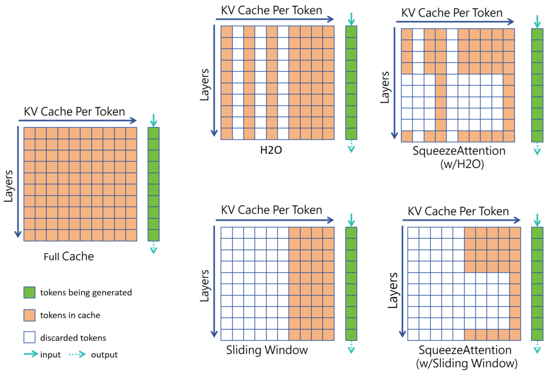
Figure 1: Demonstrations of KV-cache policies in inference from the view of the sequence and attention layer. Full Cache (leftmost column) simply stores the KV embeddings for all the tokens in all the layers. Intra-layer compression algorithms (middle column) drop tokens in the sequence’s dimension, where each layer has the same cache budget. SqueezeAttention (rightmost column) further compresses the KV-cache by adaptively re-allocating the cache budgets in the layer’s dimension.

1 Introduction

The remarkable performance achieved by generative large language models (LLM) across a wide range of natural language processing (NLP) tasks is making people in the computing industry believe that it has a great potential to reshape the way they design their products. The past year has witnessed an unprecedented surge in applications driven by LLMs, such as intelligent chatbots, LLM-powered search engines, digital personal assistants, automatic programming tools, and so on. Along with the ever-growing LLM applications, their massive inference cost starts becoming a severe challenge that hinders the deployment of LLMs and raises concerns regarding their carbon footprint Faiz et al. (2023).

For a decoder-only autoregressive model, which is the most widely adopted LLM architecture, the inefficiencies in inference mainly come from the fact that the model can only generate tokens one by one, and sampling each token requires attending to all previous tokens. In practice, the intermediate key-value embeddings of each layer have been cached incrementally in each iteration to avoid frequent recomputations. Since the KV-cache increases linearly with the number of attention layers, context length and batch size, it often ends up being multiple times larger than the model itself Sheng et al. (2023), and therefore, dominating the I/O cost of inference. Recently, optimizing the KV-cache has been broadly considered a critical approach to boost the efficiency of inference. From the perspective of context length, many well-studied algorithms are trying to identify the most "valuable" tokens in the sequence and evict the unimportant ones to reduce the KV-cache and attention complexity, such as Sliding Window Attention Beltagy et al. (2020), Heavy-Hitter (H2O) Zhang et al. (2024), StreamingLLM Xiao et al. (2023), Scissorhands Liu et al. (2024), FastGen Ge et al. (2023) and so on. From the perspective of batching, many studies aim to explore how to efficiently manage the memory of KV-cache on a batch basis with different sequence lengths Zheng et al. (2023); Kwon et al. (2023). However, the opportunities in the dimension of attention layers have barely been touched by most, if not all, of the existing methods. In other words, all the attention layers have always been treated equally by those KV caching strategies. Therefore, in this paper we ask:

Do all the attention layers necessarily have to store the same amount of KV-cache? If not, how can we precisely reallocate the cache budget for each layer such that we can further reduce the KV-cache in total?

To answer these questions, we need to take a closer look at the behaviors of different attention layers during inference. Some inspiring clues could be found in a few related studies. Early-exiting LLM Del Corro et al. (2023), as a widely-adopted inference method, shows that after going through a certain number of attention layers, the hidden representations are likely to reach saturation, and therefore, the forward computing can exit early without finishing the entire network and still get a reasonable prediction. Besides, a very recent work called FastGen Ge et al. (2023) found that attention layers in different positions have quite different preferences regarding KV caching policies. For example, attention heads in the first and last layers prefer caching all the tokens in the sequence, whereas, some middle layers prefer caching only frequent and special tokens. These insights indicate that attention layers do have quite different degrees of importance regarding inference, encouraging us to make a hypothesis that by taking advantage of the layer importance we could further "squeeze" the KV-cache that has already been optimized by those existing intra-layer algorithms, from the layer’s dimension, and eventually, achieve even better efficiencies.

To describe the importance of the attention layers quantitatively, we track the cosine similarity, which has been considered a robust metric to reflect the similarity of embeddings in NLP Sidorov et al. (2014), between the hidden representations before and after the self-attention computing in each layer, and then put all layers’ data together to demonstrate how an input embedding evolves through the entire model in inference. The intuition is that the more similar the embeddings are after the attention computing (indicated by higher cosine similarity), the less information this attention layer could insert into the embedding. After broad investigations into multiple popular LLM models, e.g., Mistral-7B, Falcon-7B, Llama2-7B, Llama2-70B, and so on, as shown in Figure 2, we found some common characteristics. Firstly, the first half of attention layers, in general, contributes more to the output embedding than what second half does. Secondly, some specific layers, typically the first and last few layers, might be more important than other layers, depending on the specific model and dataset.

Based on this simple yet effective indicator, we propose SqueezeAttention, a 2D KV-cache compression algorithm that prunes KV-cache from not only the sequence’s dimension but also the layer’s dimension. Since the layer importance is highly dependent on the model and task, SqueezeAttention categorizes all the layers into groups on the fly by clustering their cosine similarities measured during the prompt prefilling phase. Given an intra-layer KV-cache compression policy (like Sliding Window Beltagy et al. (2020) or H2O Zhang et al. (2024)), and a unified cache budget (like 4096 tokens or 20% of prompt length), SqueezeAttention automatically reallocates the cache budgets among groups of layers such that the important layers could cache more tokens to stabilize the model accuracy and the unimportant layers could drop more unnecessary tokens to save the I/O cost. What’s even better is that SqueezeAttention is orthogonal to all those intra-layer KV-cache compression algorithms, so it can be smoothly combined with any of them. Figure 1 demonstrates how the SqueezeAttention works jointly with two representative KV compression algorithms, i.e., H2O Zhang et al. (2024) and Sliding Window Attention Beltagy et al. (2020). More details about the SqueezeAttention algorithm can be found in Section 4.

To the best of our knowledge, SqueezeAttention is the first algorithm considering the KV-cache budget in a layer-wise way, making it a valuable addition to all those sequence-wise sparsification algorithms for inference. In our experiments, we integrate SqueezeAttention into 7 popular LLM models, i.e., Llama2-7B, Mistral-7B, Falcon-7B, OPT-6.7B, GPT-Neox-20B, Mixtral-8$\times$7B, and Llama2-70B, combining with 3 representative intra-layer KV-cache compression algorithms, i.e., Heavy-Hitter Oracle (H2O), Sliding Window Attention and StreamingLLM. The results show that SqueezeAttention can achieve better model performance with even lower cache budgets than all three algorithms under a wide range of models and tasks, which lead to approximately 30% to 70% of the memory savings and up to 2.2 $\times$ of throughput improvements for inference.

2 Preliminaries and Related Work

2.1 Anatomy of KV-cache in LLM Inference

For a decoder-only transformer-based model, the inference process typically involves two phases: prefilling and decoding. In prefilling, LLM takes the entire prompt as input to calculate and cache the key-value embeddings of each token in each attention layer. Then the decoding phase takes one embedding at a time to generate tokens by iterations, and meanwhile, concatenates the newly calculated KV embedding to the KV-cache.

Let $p$ be the length of the prompt, $o$ be the length of the output, $b$ be the batch size, $n_{layer}$ be the total number of attention layers, and $d_{model}$ be the hidden dimension. In the $i$-th layer, denote the model weights regarding attention Key and Value by $\textbf{w}_{K}^{i}$ and $\textbf{w}_{V}^{i}$, where $\textbf{w}_{K}^{i}\in\mathbb{R}^{d_{model}\times d_{model}}$, and $\textbf{w}_{V}^{i}\in\mathbb{R}^{d_{model}\times d_{model}}$.

In the prefilling phase, denote the hidden states of the $i$-th layer by $\textbf{h}_{prompt}^{i}$, where $\textbf{h}_{prompt}^{i}\in\mathbb{R}^{b\times p\times d_{model}}$. Then the KV-cache of the $i$-th layer after prefilling can be formulated as:

$$\textbf{C}_{K}^{i}=\textbf{h}^{i}_{prompt}\cdot\textbf{w}_{K}^{i};\textbf{C}_{V}^{i}=\textbf{h}^{i}_{prompt}\cdot\textbf{w}_{V}^{i}$$ (1)

In the decoding phase, denote the hidden states of the $j$-th output token in $i$-th layer by $\textbf{h}_{output_{j}}^{i}$ ($1\leqslant j\leqslant o$), where $\textbf{h}_{output_{j}}^{i}\in\mathbb{R}^{b\times 1\times d_{model}}$. Then the KV-cache of the $i$-th layer after generating $j$-th tokens can be formulated as:

$$\textbf{C}_{K}^{i}=\texttt{CONCAT}(\textbf{C}_{K}^{i},\textbf{h}_{output_{j}}^{i}\cdot\textbf{w}_{K}^{i})$$ (2)

$$\textbf{C}_{V}^{i}=\texttt{CONCAT}(\textbf{C}_{V}^{i},\textbf{h}_{output_{j}}^{i}\cdot\textbf{w}_{V}^{i})$$ (3)

As the decoding process goes along, KV-cache is growing incrementally until the output sequence is fully finished. Therefore, the maximum number of floats in total of the KV-cache is:

$$2\cdot\sum^{n_{layer}}_{i=1}[b\cdot(p+o)\cdot d_{model}]$$ (4)

or simply $2\cdot d_{model}\cdot n_{layer}\cdot b\cdot(p+o)$.

Taking Llama-2-7B in FP16 as an example, where $n_{layer}=32$, $d_{model}=4096$. The entire model weights consumes around 14GB of memory, whereas, the KV-cache takes around 0.5MB per token. In other words, the KV-cache starts to exceed model weights when processing more than 28K tokens, which could be easily made up of a batch of 28 requests with 1K content length.

2.2 Existing KV-cache Optimizations

As analyzed above, the number of layers, batch size, and context length are three critical factors that decide the size of the KV-cache. Therefore, existing optimization studies are likely to seek opportunities from these perspectives.

Sparsifying the context sequence is an effective way to break the linear relationship between the context length and the KV-cache Del Corro et al. (2023); Zhang et al. (2024); Anagnostidis et al. (2023); Sukhbaatar et al. (2019); Rae and Razavi (2020). The general intention of these algorithms is to find out the unimportant tokens in the sequence and drop the KV-cache of these tokens. For example, Sliding Window Attention Beltagy et al. (2020) only caches a certain number of the most recent tokens and drops the rest. StreamingLLM Xiao et al. (2023) found that in addition to the recent tokens, tokens at the beginning of the sequence are also crucial to the output. Heavy-Hitter Zhang et al. (2024) and Scissorhands Liu et al. (2024) rank the importance of tokens by comparing their attention scores. As mentioned above, these algorithms treat all the attention layers equally, and therefore, have a fixed KV-cache budget for each layer.

Optimizing the KV-cache on a batch basis mainly needs to manage the memory of different requests efficiently. For example, vLLM Kwon et al. (2023) allocates small chunks of memory in an on-demand way, instead of a fixed big block for each prompt, to reduce the memory fragmentation in a batch. RadixAttention Zheng et al. (2023) manages to share the KV-cache across requests in a batch when they have the same prefix in the prompt.

Last but not least, how to relax the linear relationship between the KV-cache and the layers remains largely unexplored compared with the other two dimensions. FastGen Ge et al. (2023) is a very recent work that found layers in different positions may have different preferences on the KV-cache policies. It then proposed an algorithm to choose the best cache policy for each attention head during the inference. Note that FastGen aims to find out the optimal cache policy for attention heads, but all the heads sharing the same policy still simply have the same cache budget, like 30% of the most recent tokens, which makes SqueezeAttention still orthogonal to it.

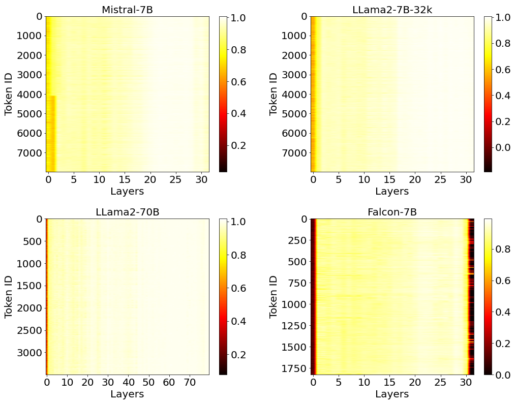
Figure 2: Visualization of cosine similarity before and after the self-attention calculation of attention each layer. The layers with higher cosine similarity, represented by lighter colors, exert a relatively lower impact on the input vectors.

3 Observations

Inspired by some previous works that managed to optimize the LLM inference from a layer-wise perspective Del Corro et al. (2023); Ge et al. (2023), we make a hypothesis that attention layers in different positions play distinct roles in terms of importance, and therefore, should have different optimal KV-cache budgets. To better understand the layer-wise contribution to the output embedding, we employ cosine similarity as the metric to quantify the importance of each layer during inference. Specifically, in each attention layer, we track the hidden states of each input embedding at two spots, i.e., the embedding before and after the self-attention block. Denote the hidden state before the self-attention by $\mathbf{A}$, and the hidden state after the self-attention by $\mathbf{B}$. The cosine similarity between two embeddings $\mathbf{A}$ and $\mathbf{B}$ is calculated as follows:

$$\text{CosineSimilarity}(\mathbf{A},\mathbf{B}) =\frac{\mathbf{A}\cdot\mathbf{B}}{\|\mathbf{A}\|\cdot\|\mathbf{B}\|}$$ (5)

$$=\frac{\sum\limits_{i=1}^{n}A_{i}\cdot B_{i}}{\sqrt{\sum\limits_{i=1}^{n}A_{i}^{2}}\cdot\sqrt{\sum\limits_{i=1}^{n}B_{i}^{2}}}$$ (6)

where $\mathbf{A}=(A_{1},A_{2},\ldots,A_{n})$ and $\mathbf{B}=(B_{1},B_{2},\ldots,B_{n})$ are the vectors, and $n$ is the dimensionality.

For any given input embedding, we could get a cosine similarity of each attention layer that roughly quantifies how much the embedding changes after the self-attention computing of this layer. Then by comparing the cosine similarity among layers, we could find a way to rank attention layers by their importance. Following this line of thought, we choose 4 representative LLMs, i.e., Mistral-7B Jiang et al. (2023), Llama2-7B-32K Touvron et al. (2023), Llama2-70B Touvron et al. (2023), Falcon-7B Almazrouei et al. (2023), to conduct the experiments. Each model is fed by 200 prompts and we track the cosine similarity of each token in each layer. Figure 2 shows the results after averaging over prompts. Each row of the heatmap demonstrates how an input embedding at the given position evolves through all the layers. From the brightness of the figures, we can get some insights as follows: 1) In general, the first half of layers (in a darker color) contributes more to the output embeddings than the second half of layers (in a lighter color) does; 2) The first and last few layers tend to be more critical than other layers, depending on the specific models and tasks; 3) The cosine similarity can effectively depict the layer-wise importance, as the trend it reflects aligns with the previous studies, like Early-exiting Del Corro et al. (2023) and FastGen Ge et al. (2023).

This observation gives us a simple yet effective metric to design a new algorithm that is able to optimize the KV-cache from not only the context’s dimension, but also the layer’s dimension.

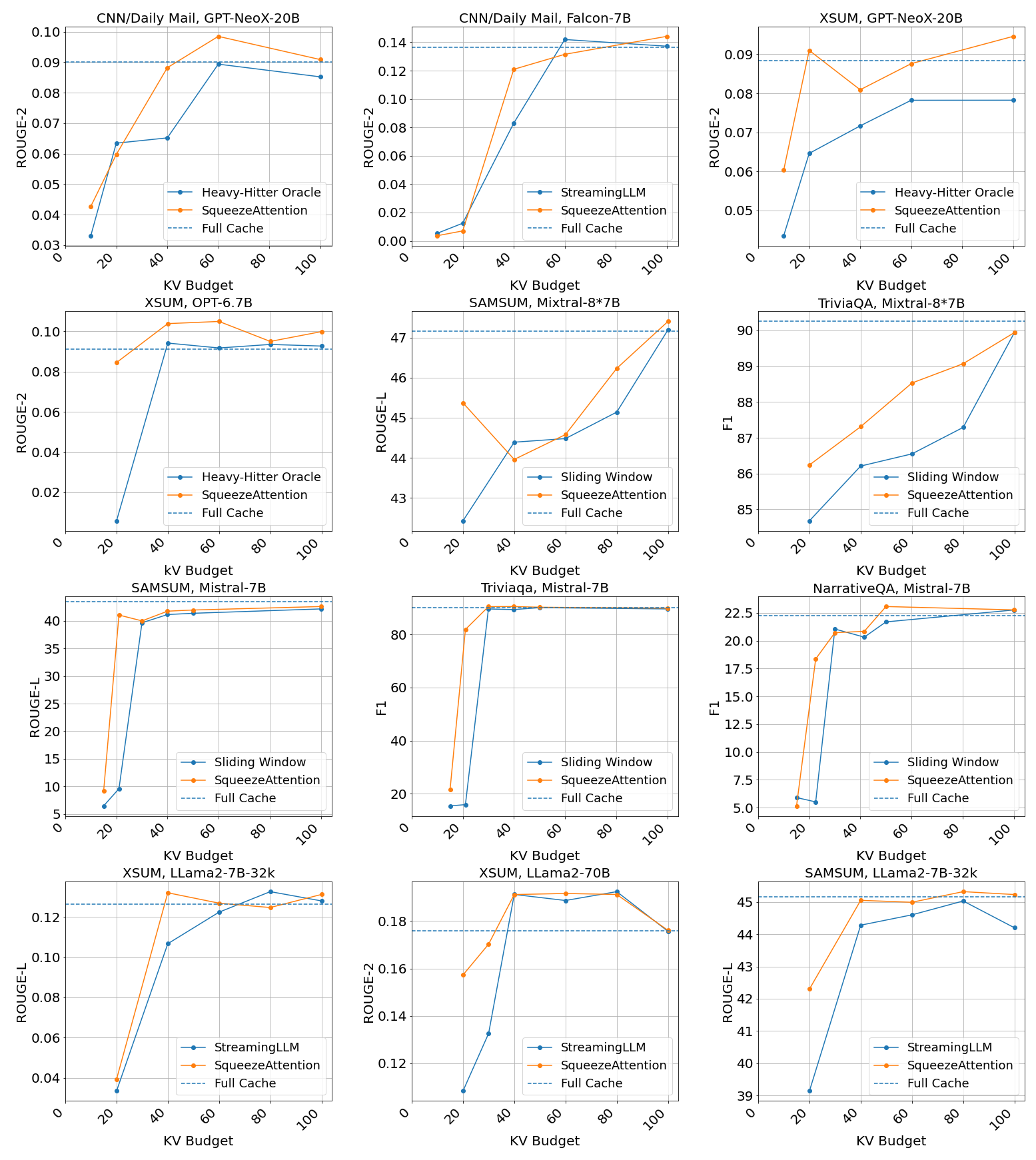
Figure 3: Performance of SqueezeAttention, baseline algorithms, and Full Cache under different cache budgets.

4 Algorithm

In this section, we describe the SqueezeAttention algorithm inspired by our observations from the last chapter. The most distinct feature of the proposed algorithm is that it considers tokens in the KV-cache as a 2D matrix with one dimension of sequence and another dimension of layer, and both dimensions are going to be optimized jointly.

In the sequence’s dimension, there are various cache eviction policies that we could directly combine with, like Least Recently Used methods (Sliding Window, StreamingLLM), Least Frequently Used methods (Scissorhands, H2O), and so on. We denote a policy that compresses the KV-cache in sequence’s dimension by $\boldsymbol{C}_{seq}$, and its cache budget by $b_{init}$. Note that all the layers have the same cache budget by default, just like the assumptions made by all these intra-layer KV compression algorithms.

In the layer’s dimension, SqueezeAttention firstly tracks the layer importance with the given prompt in the prefilling phase by collecting the cosine similarities of each layer whenever the self-attention is conducted. At the end of prefilling, each layer ends up with a set of cosine similarities, each of which corresponds to a token that has flowed through this layer. Then we use the averaged value over prompt tokens to represent the layer-wise importance of this layer regarding this task. By clustering the layers into groups based on the layer-wise importance with KMeans, we reallocate the $b_{init}$ for each layer in a way that more budgets are assigned to the more "important" layer groups. Since layers have different cache budgets, in the decoding phase, $\boldsymbol{C}_{seq}$ works separately with each layer’s very own budgets. The detailed process is described in Algorithm 1.

Algorithm 1 SqueezeAttention

1:$prompt$: input sequence; $\boldsymbol{C}_{seq}$: a KV-cache compressor in sequence dimension; $b_{init}$: the initial cache budget of each layer; $n_{layer}$: number of attention layers; $p$: hyperparameter ($0<p<1$); $K^{(i)}$: KV-cache of the $i$-th layer;

2:Feed the $prompt$ into the model for prefilling, calculate $cos\_sim^{(i)}_{j}$ of the $j$-th token in the $i$-th layer by Equation 5;

3:for $i\leftarrow$ 1 to $n_{layer}$ do

4:     $cos\_sim^{(i)}=\frac{\sum_{j=1}^{\texttt{len}(prompt)}cos\_sim^{(i)}_{j}}{\texttt{len}(prompt)}$

5:end for

6:$G_{1},G_{2},G_{3}\leftarrow$ KMeans($cos\_sim^{(i)}$)$\triangleright$ Cluster layers into 3 groups by $cos\_sim^{(i)}(1\leqslant i\leqslant n_{layer})$, where $G_{3}$ has the biggest $cos\_sim$ on average

7:for $i\leftarrow 1$ to $n_{layer}$ do

8:     if $i\in G_{3}$ then

9:         $b^{(i)}=b_{init}\times p$

10:     else

11:         $b^{(i)}=\frac{n_{layer}\times b_{init}-\texttt{len}(G_{3})\times b_{init}\times p}{\texttt{len}(G_{1})+\texttt{len}(G_{2})}$

12:     end if

13:     $K^{(i)}=\texttt{KV}(prompt)$$\triangleright$ the prompt’s KV is cached after prefilling

14:end for

15:for $o\leftarrow 1$ to $\texttt{len}(output)$ do$\triangleright$ Decoding output tokens one by one

16:     for $i\leftarrow 1$ to $n_{layer}$ do

17:         if $\texttt{len}(K^{(i)})>b^{(i)}$ then

18:              $K^{(i)}=\boldsymbol{C}_{seq}(K^{(i)},b^{(i)})$ $\triangleright$ Compress the KV-cache of this layer by its own budget

19:         end if

20:         Finish the Self-attention based on the compressed $K^{(i)}$.

21:     end for

22:end for

Discussions. SqueezeAttention involves a hyperparameter $p$ to control the percentage of initial budgets that could be removed from the "unimportant" layers. The bigger the $p$ is, the more budgets will be reassigned. In experiments, we found 0.1-0.2 is a reasonable choice range in most cases. Empirically, we cluster layers into 3 groups. Group 1 (smallest similarity) usually stands for a few special layers, like the first and last layers, whose similarities are way lower than other layers. Group 3 (biggest similarity, typically between 0.95 to 0.99) represents the layers that barely make any difference to the embeddings after the self-attention. Group 2 is in the middle. To preserve the model accuracy, we only reduce cache budgets from Group 3, which accounts for around 50% to 70% of total layers.

Table 1: Datasets used in our experiments.

Task	Task Type	Eval metric	Avg len	Language	Sample
CNN/ Daily Mail	Summarization (3 sentence)	Rouge-2	2,000	EN	1,000
XSUM	Summarization (1 sentence)	Rouge-2	2,000	EN	1,000
SAMSUM	Few shot	Rouge-L	6,258	EN	200
NarrativeQA	Single-doc QA	F1	18,409	EN	200
TriviaQA	Few shot	F1	8,209	EN	200

Table 2: Performance among Full cache, SqueezeAttention and Baseline Algorithms.

Model	Size	Dataset	Baseline Algorithm	Performance / Used KV Budget
				Full Cache	SqueezeAttention	Basic Algorithm
Mistral	7B	SAMSUM	Sliding Window	43.53 / 100%	41.05 / 20%	40 / 30%
GPT-NeoX	20B	XSUM	Heavy-Hitter Oracle	0.09 / 100%	0.09 / 20%	0.08 / 60%
LLama2	70B	XSUM	StreamingLLM	0.18 / 100%	0.17 / 30%	0.19 / 40%

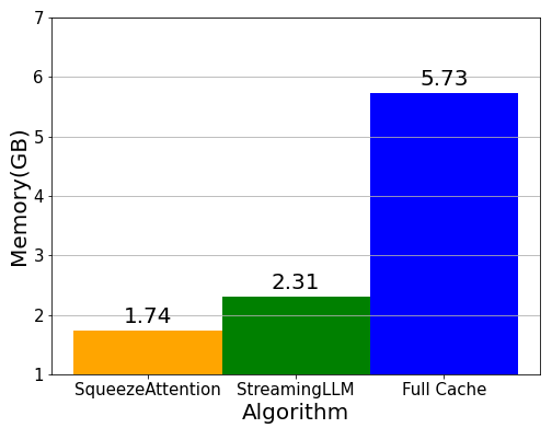
(a) LLama2-70B

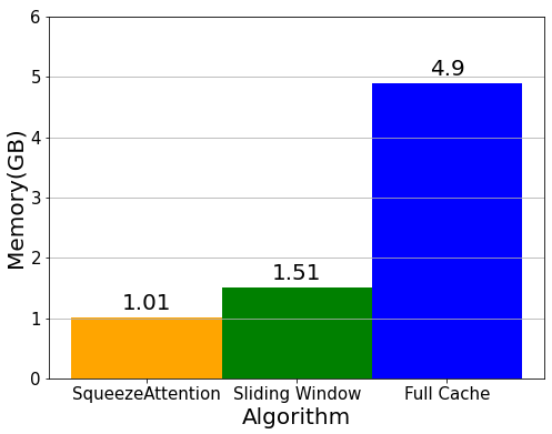
(b) Mistral-7B

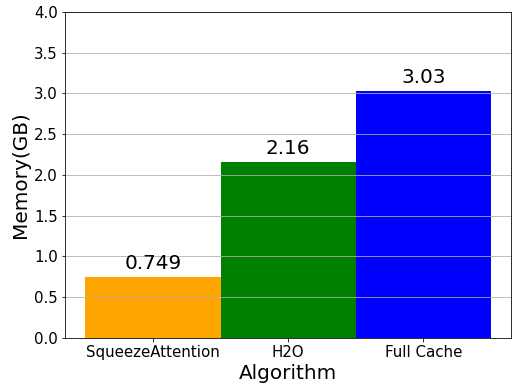
(c) GPT-NeoX-20B

Figure 4: Comparisons of per-token decoding memory usage among the Full cache, SqueezeAttention, and baseline algorithms, all methods achieve similar accuracies shown in Table LABEL:accuary_result.

5 Experiments

In this section, we evaluate the SqueezeAttention on a wide range of LLM models and datasets. We choose 3 state-of-the-art sequence-wise compression algorithms as baselines, and show how our algorithm works jointly with them to achieve even better performance regarding the model accuracy and hardware efficiency.

5.1 Experiment Setup

LLM Models. We choose 7 representative LLMs, with model sizes ranging from 6.7B to 70B and context lengths ranging from 2K to 32K, to evaluate the proposed algorithm: GPT-NeoX-20B, OPT-6.7B, Falcon-7B, Mistral-7B, Mixtral-8$\times$7B, LLama2-7B-32k, LLama2-70B.

Datasets. We conduct experiments on 5 datasets: CNN/Daily Mail, XSUM, TriviaQA, SAMSUM, and NarrativeQA. TriviaQA, SAMSUM, and NarrativeQA originate from LongBench Bai et al. (2023), where the data length typically exceeds 8k. CNN/Daily Mail and XSUM have an average length of about 2k. Detailed information about datasets can be found in Table 1.

Baselines. 3 sequence-wise sparsification algorithms are chosen as the baselines to integrate into SqueezeAttention:

• Heavy-Hitter (H2O): Identify the important tokens within the sequence by comparing the accumulated attention score of each token.

• Sliding Window Attention: A "Local" strategy that only caches the most recent tokens’ KV embeddings. This method works especially well with Mistral and Mixtral.

• StreamingLLM: In addition to the most recent tokens, StreamingLLM always caches the first $n$ tokens in the sequence, as they are identified as "sink tokens". We take $n=4$ as recommended by the paper.

Hardwares. We conduct all the experiments on the AWS platform (p4d.24xlarge) with 8 Nvidia A100-40GB GPUs, interconnected by the NVLinks (600 GB/s GPU peer-to-peer bandwidth).

5.2 End-to-End Result

Figure 3 demonstrates the comparison results of SqueezeAttention and other 3 baseline algorithms over all 7 models and 5 datasets. Full Cache (dashed line) means all tokens’ KV embeddings are fully cached during the inference, therefore, it represents a relatively good model accuracy. The blue and orange curves in each subfigure illustrate how the model accuracy changes with the KV-cache budgets ranging from 10% to 100% of the total sequence length. For each model, we choose the best sequence-wise compression algorithm to represent the best case of intra-layer optimization, and then use SqueezeAttention on top of the best case. As shown in the figure, SqueezeAttention consistently manages to improve the model accuracies under various KV-cache budgets by reallocating the cache budgets among layers. In other words, SqueezeAttention can achieve similar inference accuracies with much less KV-cache in total.

Table 3: Generation throughput (token / s) on eight A100 GPUs of Mistral-7B and LLama2-70B with SqueezeAttention and Full Cache. To maintain the model accuracy, SqueezeAttention uses 20% of the cache budget for Mistral-7B and 30% of the cache budget for LLama2-70B. "OOM" means out-of-memory.

Model	Size	prompt len + gen len	Algorithm	Batch size
				1	32	64	128	224
Mistral	7B	512 + 1024	SqueezeAttention	20.5	496.5	682.7	824.4	892.5
			Full Cache	20.9	254.0	304.8	OOM	OOM
Model	Size	prompt len + gen len	Algorithm	Batch size
				1	8	16	32	64
LLama2	70B	256 + 512	SqueezeAttention	5.2	37.2	71.2	116.2	170.7
			Full Cache	5.2	36.0	62.5	84.8	OOM

5.3 Memory Consumption

Now we evaluate the memory consumption of the proposed algorithm. We choose three settings to compare how much GPU memory it needs to run the inference without degradation of model accuracy. We select Mistral-7B (Sliding Window), GPT-NeoX-20B (Heavy-Hitter), and LLama2-70B (StreamingLLM) to cover all three baseline algorithms and models in small, middle, and large sizes. We utilize multi-GPU inference if the model and KV-cache do not fit into a single GPU.

Table LABEL:accuary_result demonstrates that in all three settings, by achieving the same model accuracy, SqueezeAttention consumes the least amount of KV-cache budgets compared with the algorithms that only compress from the sequence’s dimension. In some cases, it only takes one-third of the cache budget of H2O algorithm. Subsequently, we employ PYTORCH PROFILER to evaluate the diminished memory usage of generating one token during the inference (w/o memory usage of model weights). Figure 4 shows that SqueezeAttention can save 70% to 80% of memory usage per token compared with Full Cache method, and 25% to 66% of memory usage compared with baseline algorithms.

5.4 Throughput of Token Generation

Since SqueezeAttention manages to save the memory cost of inference, as shown in the previous sections. Now we want to explore how these memory reductions can be interpreted into improvements of token throughput. We choose 2 models, i.e., Mistral-7B and Llama-70B, to represent models in different sizes. With a fixed content length, we increase the batch size from 1 to 224 for Mistral-7B, and 1 to 64 for Llama2. For each task, we select the best setting for the SqueezeAttention, that is, Sliding Window for Mistral-7B and StreamingLLM for Llama2-70B.

Table LABEL:throughput_result shows the token throughput on 8 A100-40GB GPUs. With the same batch size, SqueezeAttention can enhance throughput by up to 2.2$\times$ for Mistral-7B and 1.4$\times$ for Llama2-70B compared to the Full Cache. Besides, SqueezeAttention also enables batch sizes up to 224 and 64 for two models, which would cause out-of-memory for the Full Cache method.

6 Conclusion

In this paper, we propose a 2D KV-cache compression algorithm called SqueezeAttention. By tracking the cosine similarity of each attention layer, we found that layers in different positions have distinct degrees of importance regarding the output embedding. Inspired by this observation, SqueezeAttention reallocates the KV-cache budgets over attention layers to further reduce the memory cost of inference. Experiments over a wide range of models and tasks show that SqueezeAttention can achieve better model accuracies with lower memory consumption compared with SOAT algorithms that only compress KV-cache from one dimension.

References

- Almazrouei et al. (2023) Ebtesam Almazrouei, Hamza Alobeidli, Abdulaziz Alshamsi, Alessandro Cappelli, Ruxandra Cojocaru, Merouane Debbah, Etienne Goffinet, Daniel Heslow, Julien Launay, Quentin Malartic, Badreddine Noune, Baptiste Pannier, and Guilherme Penedo. 2023. Falcon-40B: an open large language model with state-of-the-art performance.
- Anagnostidis et al. (2023) Sotiris Anagnostidis, Dario Pavllo, Luca Biggio, Lorenzo Noci, Aurelien Lucchi, and Thomas Hoffmann. 2023. Dynamic context pruning for efficient and interpretable autoregressive transformers. arXiv preprint arXiv:2305.15805.
- Bai et al. (2023) Yushi Bai, Xin Lv, Jiajie Zhang, Hongchang Lyu, Jiankai Tang, Zhidian Huang, Zhengxiao Du, Xiao Liu, Aohan Zeng, Lei Hou, et al. 2023. Longbench: A bilingual, multitask benchmark for long context understanding. arXiv preprint arXiv:2308.14508.
- Beltagy et al. (2020) Iz Beltagy, Matthew E Peters, and Arman Cohan. 2020. Longformer: The long-document transformer. arXiv preprint arXiv:2004.05150.
- Del Corro et al. (2023) Luciano Del Corro, Allie Del Giorno, Sahaj Agarwal, Bin Yu, Ahmed Awadallah, and Subhabrata Mukherjee. 2023. Skipdecode: Autoregressive skip decoding with batching and caching for efficient llm inference. arXiv preprint arXiv:2307.02628.
- Faiz et al. (2023) Ahmad Faiz, Sotaro Kaneda, Ruhan Wang, Rita Osi, Parteek Sharma, Fan Chen, and Lei Jiang. 2023. Llmcarbon: Modeling the end-to-end carbon footprint of large language models. arXiv preprint arXiv:2309.14393.
- Ge et al. (2023) Suyu Ge, Yunan Zhang, Liyuan Liu, Minjia Zhang, Jiawei Han, and Jianfeng Gao. 2023. Model tells you what to discard: Adaptive kv cache compression for llms. arXiv preprint arXiv:2310.01801.
- Jiang et al. (2023) Albert Q Jiang, Alexandre Sablayrolles, Arthur Mensch, Chris Bamford, Devendra Singh Chaplot, Diego de las Casas, Florian Bressand, Gianna Lengyel, Guillaume Lample, Lucile Saulnier, et al. 2023. Mistral 7b. arXiv preprint arXiv:2310.06825.
- Kwon et al. (2023) Woosuk Kwon, Zhuohan Li, Siyuan Zhuang, Ying Sheng, Lianmin Zheng, Cody Hao Yu, Joseph E. Gonzalez, Hao Zhang, and Ion Stoica. 2023. Efficient memory management for large language model serving with pagedattention. In Proceedings of the ACM SIGOPS 29th Symposium on Operating Systems Principles.
- Liu et al. (2024) Zichang Liu, Aditya Desai, Fangshuo Liao, Weitao Wang, Victor Xie, Zhaozhuo Xu, Anastasios Kyrillidis, and Anshumali Shrivastava. 2024. Scissorhands: Exploiting the persistence of importance hypothesis for llm kv cache compression at test time. Advances in Neural Information Processing Systems, 36.
- Rae and Razavi (2020) Jack W Rae and Ali Razavi. 2020. Do transformers need deep long-range memory. arXiv preprint arXiv:2007.03356.
- Sheng et al. (2023) Ying Sheng, Lianmin Zheng, Binhang Yuan, Zhuohan Li, Max Ryabinin, Beidi Chen, Percy Liang, Christopher Ré, Ion Stoica, and Ce Zhang. 2023. Flexgen: High-throughput generative inference of large language models with a single gpu. In International Conference on Machine Learning, pages 31094–31116. PMLR.
- Sidorov et al. (2014) Grigori Sidorov, Alexander Gelbukh, Helena Gómez-Adorno, and David Pinto. 2014. Soft similarity and soft cosine measure: Similarity of features in vector space model. Computación y Sistemas, 18(3):491–504.
- Sukhbaatar et al. (2019) Sainbayar Sukhbaatar, Edouard Grave, Piotr Bojanowski, and Armand Joulin. 2019. Adaptive attention span in transformers. arXiv preprint arXiv:1905.07799.
- Touvron et al. (2023) Hugo Touvron, Louis Martin, Kevin Stone, Peter Albert, Amjad Almahairi, Yasmine Babaei, Nikolay Bashlykov, Soumya Batra, Prajjwal Bhargava, Shruti Bhosale, et al. 2023. Llama 2: Open foundation and fine-tuned chat models. arXiv preprint arXiv:2307.09288.
- Xiao et al. (2023) Guangxuan Xiao, Yuandong Tian, Beidi Chen, Song Han, and Mike Lewis. 2023. Efficient streaming language models with attention sinks. arXiv preprint arXiv:2309.17453.
- Zhang et al. (2024) Zhenyu Zhang, Ying Sheng, Tianyi Zhou, Tianlong Chen, Lianmin Zheng, Ruisi Cai, Zhao Song, Yuandong Tian, Christopher Ré, Clark Barrett, et al. 2024. H2o: Heavy-hitter oracle for efficient generative inference of large language models. Advances in Neural Information Processing Systems, 36.
- Zheng et al. (2023) Lianmin Zheng, Liangsheng Yin, Zhiqiang Xie, Jeff Huang, Chuyue Sun, Cody Hao Yu, Shiyi Cao, Christos Kozyrakis, Ion Stoica, Joseph E Gonzalez, et al. 2023. Efficiently programming large language models using sglang. arXiv preprint arXiv:2312.07104.