Nonreciprocal Nonlinear Responses in the Nonequilibrium States: Moving Charge Density Waves

Abstract

The incommensurate charge density wave states (CDWs) can exhibit steady motion in the flow limit after depinning, behaving as a nonequilibrium system with time-dependent states. Since the moving CDW, like an electric current, breaks both time-reversal and inversion symmetries, one may speculate the emergence of nonreciprocal nonlinear responses from such motion. However, the moving CDW order parameter is intrinsically time-dependent in the lab frame, and it is known to be challenging to evaluate the responses of such a time-varying system. In this work, following the principle of Galilean relativity, we resolve this time-dependent hard problem in the lab frame by mapping the system to the comoving frame with static CDW states through the Galilean transformation. We explicitly show that the nonreciprocal nonlinear responses would be generated by the movement of CDW states through violating Galilean relativity. Our work demonstrates not only nonreciprocal nonlinear responses in nonequilibrium states but also the application of Galilean transformation in simplifying time-dependent problems.

Introduction.— Nonreciprocal nonlinear responses can manifest when inversion symmetry (and time-reversal symmetry in many cases) is broken [1, 2]. These phenomena have garnered significant theoretical and experimental attention in recent years, notably in phenomena such as nonlinear Hall effects [3, 4] and nonreciprocal superconducting effects [5, 6, 7, 2]. However, while much focus has been near the equilibrium states, nonreciprocal nonlinear responses in nonequilibrium systems with time-dependent states remain largely unexplored. Theoretical investigation of such responses in nonequilibrium states is challenging due to the inherent time dependence and dynamic nature of these systems.

In condensed matter physics, current-driven systems can exhibit nonequilibrium behavior and intrinsic time-dependence. For example, certain symmetry-breaking orders would undergo motion once they surpass impurity-pinning effects under an electric field beyond the threshold. A notable example is the incommensurate charge density wave (CDW), where intriguing dynamical properties emerge upon depinning [8, 9, 10, 11, 12]. In the limit of large current, these CDW states flow steadily, representing a nonequilibrium steady state.

A CDW motion breaks both inversion and time-reversal symmetries (see illustrations in Figs. 1 (a) and (c)), as implied in the seminar work by Allender, Bray, and Bardeen [13]. One may naturally ask whether there are any finite nonreciprocal nonlinear responses induced by the current-driven motion [Fig. 1(a)]. However, directly addressing this problem is challenging due to the intrinsic time dependence of a moving CDW in the lab frame.

On the other hand, in classical physics, we know that the principle of relativity is often powerful in simplifying a problem by changing inertial frames. Following this principle, the moving CDW problem can be reconsidered in the comoving frame, where the CDW state becomes static. In contrast to the lab frame, the asymmetry induced by the external current appears to vanish in the comoving frame as illustrated in Figs. 1 (b) and (d). As a result, one may expect that nonreciprocal nonlinear responses vanish in the comoving frame. Looking at the nonreciprocal nonlinear responses for moving states within both the lab and comoving frame is indeed puzzling but important in this field [12, 13, 14].

Motivated by exploring nonreciprocal nonlinear responses in nonequilibrium systems with time-dependent state and the aforementioned puzzle, we explicitly study nonreciprocal nonlinear responses in moving CDW states in this work. We begin with a simple one-dimensional (1D) CDW model, where the CDW order parameter moves spatially at a constant velocity. Using the field theory approach, we identify that the moving CDW state can be mapped to a static one through the Galilean transformation. The transformation is identical to the change of inertial frames from the lab frame to the comoving frame with the CDW. We also argue that the Galilean transformation dictates the invariance of the finite conductivity in the lab and comoving frames, facilitating the straightforward solution of optical responses in the comoving frame. Based on this understanding, we show that the nonreciprocal nonlinear responses are absent with Galilean relativity, where the single-particle dispersion is simply quadratic and thus Galilean invariant. By introducing a quartic term to violate Galilean relativity, we explicitly show that nonreciprocal nonlinear responses would appear. Our work thus paves a way to study nonreciprocal nonlinear responses in nonequilibrium states through Galilean transformation and resolve the aforementioned important puzzle.

A moving CDW model and Galilean transformation.— Let us first illustrate how we can map a time-dependent problem in the lab frame onto a time-independent problem in the comoving using the principle of relativity. We start with the simplest 1D continuum model with a moving CDW, which has been widely used to study the dynamics of a CDW [12, 13, 15]:

$$\mathcal{L}=i\psi^{\dagger}\partial_{t}\psi-\frac{1}{2m}\partial_{x}\psi^{\dagger}\partial_{x}\psi-\psi^{\dagger}V(x-vt)\psi,$$ (1)

where $\partial_{x}$ denotes $\frac{\partial}{\partial x}$, $\psi(x,t)$ is a field operator for electrons, $m$ is an effective mass, and we set $\hbar=1$ in the main text. The CDW order parameter is

$$V(x-vt)=2\Delta\cos(2k_{F}(x-vt))$$ (2)

with $v$ the drift velocity of the CDW. The wave vector of the CDW is denoted as $2k_{F}$, where $k_{F}=\sqrt{2m\epsilon_{F}}$ is the Fermi wave vector at the Fermi energy $\epsilon_{F}$. The electronic energy dispersion acquires an energy gap $\Delta$ at the Fermi level, corresponding to the CDW order parameter. Such CDW states emerge in quasi-1D systems [12]. The Lagrangian density $\mathcal{L}$ describes the dynamics of quasi-1D CDW states driven by an electric current in the flow region [12, 13, 15]. We shall assume disorder effects are negligible in the flow region.

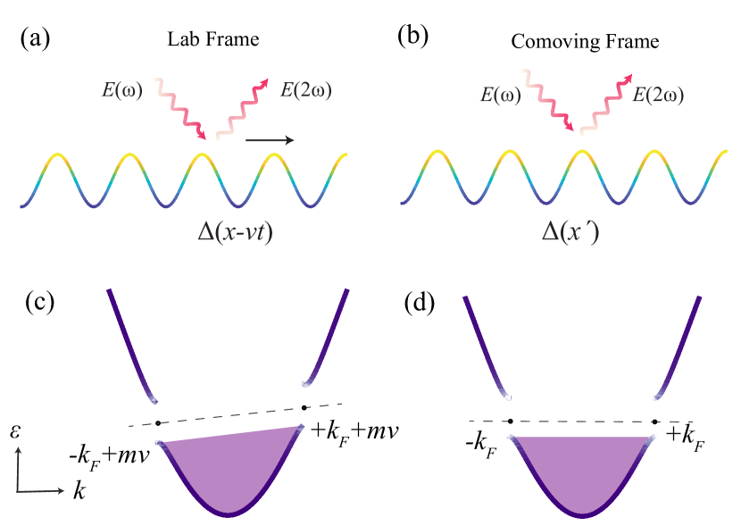
Figure 1: Illustration of the CDW states in the comoving frame and the lab frame. (a) and (b) schematically show the CDW order parameter in the comoving and lab frame, respectively. The black arrow in (a) represents the CDW motion. The possible nonreciprocal nonlinear responses induced by the moving CDW states are highlighted as the second harmonic generation. (c) shows the moving CDW states in the lab frame, where the Fermi momentum is shifted to $\pm k_{F}+mv$ and the CDW gap opens near these shifted Fermi momenta, while (d) shows the CDW states in the comoving frame, where the CDW gap opens at $\pm k_{F}$. Note that (c) cannot be simply regarded as the real energy dispersion due to the generic time-dependent feature in the lab frame.

To eliminate the time dependence of the CDW order parameter, we introduce the comoving frame by performing the Galilean transformation on the coordinates $x^{\prime}=x-vt,t^{\prime}=t$, $\partial_{t}=\partial_{t}^{\prime}-v\partial_{x^{\prime}}$, $\partial_{x}=\partial_{x^{\prime}}$. The field operator transforms as $\psi=e^{i\eta(x,t)}\psi^{\prime}$ with the phase factor $\eta(x,t)=mvx-\frac{1}{2}mv^{2}t$; see Supplementary Material (SM) Sec. I [16] for details. After this transformation, the Lagrangian in the moving frame reads

$$\mathcal{L}^{\prime}=i\psi^{\prime\dagger}\partial_{t^{\prime}}\psi^{\prime}-\frac{1}{2m}\partial_{x^{\prime}}\psi^{\prime\dagger}\partial_{x^{\prime}}\psi^{\prime}-\psi^{\prime\dagger}V(x^{\prime})\psi^{\prime}$$ (3)

with $V(x^{\prime})=2\Delta\cos(2k_{F}x^{\prime})$. Comparing Eq. (1) with Eq. (3), we can see that the exact Galilean invariance does not exist due to the CDW order parameter. However, the problem in the lab frame with the moving potential $V(x-vt)$ is mapped to the one in the comoving frame with the static potential $V(x^{\prime})$. As there are no extra new terms after Galilean transformation, we would call the system exhibits Galilean relativity in this case. Because of this Galilean relativity, the nonlinear responses would not appear since the energy dispersion is simply quadratic in the comoving frame without time dependence. Note that the uniform electric field remains unchanged during the Galilean transformation.

In general, there is no exact Galilean relativity in solids. In this work, we invoke a violation of Galilean relativity by introducing a quartic term:

$$\delta\mathcal{L}=-\lambda\partial_{x}^{2}\psi^{\dagger}\partial_{x}^{2}\psi,$$ (4)

which is allowed by any symmetries. In this case, the total Lagrangian is $\mathcal{L}_{t}=\mathcal{L}+\delta\mathcal{L}$. After the Galilean transformation, it is straightforward to show the Lagrangian in the comoving frame becomes $\mathcal{L}^{\prime}_{t}=\mathcal{L}^{\prime}+\delta\mathcal{L}^{\prime}$, where $\delta\mathcal{L}^{\prime}$ represents the quartic term in the comoving frame:

$$\delta\mathcal{L}^{\prime} =-\lambda\psi^{\prime\dagger}\partial_{x^{\prime}}^{4}\psi^{\prime}-\lambda m^{4}v^{4}\psi^{\prime\dagger}\psi^{\prime}+4i\lambda m^{3}v^{3}\psi^{\prime\dagger}\partial_{x^{\prime}}\psi^{\prime}$$ (5)

$$+6\lambda m^{2}v^{2}\psi^{\prime\dagger}\partial_{x^{\prime}}^{2}\psi^{\prime}-4i\lambda mv\psi^{\prime\dagger}\partial_{x^{\prime}}^{3}\psi^{\prime}.$$

It can be seen that when we consider a more general dispersion, beyond the simplistic quadratic band, residual terms emerge in the Lagrangian, which cannot be eliminated in the comoving frame. It is also interesting to note that the terms that are odd in momentum in Eq. (5) break inversion and time-reversal symmetries, which is expected for moving CDWs but forbidden by Galilean relativity previously. As we will see later, the cubic-momentum term, i.e., the last term in Eq. (5), results in nonreciprocal nonlinear responses.

It is worth noting that we can map the Lagrangian to be time-independent for the moving CDW model even with the quartic term via Galilean transformation. This allows us to evaluate some interesting effects that previously were hard to demonstrate in a time-dependent system. To be specific, we shall focus on the nonreciprocal nonlinear responses next.

The invariance of finite frequency responses under Galilean transformation.— We next show that the nonreciprocal nonlinear responses can be equivalently calculated in the comoving frame. The conductivity of nonlinear responses is defined by expanding the current density in the powers of external fields. For example, the $n$-th order harmonic generation in the lab frame is obtained from $J_{x}(n\omega)=\sigma_{xx}(n\omega)E^{n}_{x}(\omega)$, where $n$ is a positive integer and $\omega$ is the incident photon energy $(\hbar=1)$, $E_{x}$ denotes the electric field along $x$-direction. Note that we have simplified subscript in the conductivity; for example, the second-order conductivity tensor $\sigma_{xxx}(2\omega)$ would be simply labeled with $\sigma_{xx}(2\omega)$ or $\sigma(2\omega)$ below.

Now we show how the optical conductivity transforms upon a Galilean transformation by using the Galilean transformation relation of the electric field and current. According to the minimal coupling principle, an electromagnetic field would appear in the Lagrangian by replacing the $\partial_{i}\psi$ in Eq. (1) as $(\partial_{i}+ieA_{i})\psi$, $\partial_{i}\psi^{\dagger}$ as $(\partial_{i}-ieA_{i})\psi^{\dagger}$ [17]. Then the current-density operator is $j_{x}=\frac{\partial\mathcal{L}_{t}}{\partial A_{x}}|_{A_{x}=0}$. Upon the Galilean transformation $\psi=e^{i\eta(x,t)}\psi^{\prime}$, we find that the current-density operators in the lab and comoving frames satisfy

$$\hat{j}^{\prime}_{x}=\hat{j}_{x}+ev\psi^{\prime\dagger}\psi^{\prime},$$ (6)

where $\hat{j}_{x}^{\prime}$ is the current operator deduced from the Lagrangian $\mathcal{L}^{\prime}_{t}$. See the explicit derivations in SM Sec. III. Note that Eq. (6) holds even with the quartic term. Sandwiching the current operator with the ground state, we obtain the well-known Galilean transformation for the current

$$J^{\prime}_{x}(t)=J_{x}(t)+evN,$$ (7)

where $t^{\prime}=t$ is used and the total electron number $N=\int dx^{\prime}\braket{\psi^{\prime\dagger}\psi^{\prime}}$ , where $\braket{}$ denotes the average over the ground states. The form of Eq. (7) is consistent with the one obtained from the relativity theory in classical electrodynamics (SM Sec. II). Moreover, as shown in SM Sec.III, we argue that Eq. (7) holds for a generic energy dispersion by performing Galilean transformation in the momentum space, where the group velocity of each electron is uniformly shifted by $v$. Operating $\int dte^{-in\omega t}$ on both sides, we find $J^{\prime}_{x}(n\omega)=J_{x}(n\omega)$ for $\omega\neq 0$. Here we consider a finite frequency response because the DC conductivity with $\omega=0$ is divergent without impurities. Note that the current $evN$ in Eq. (7) does not contribute to the finite frequency response as $N$ is time-independent due to the conservation of total electron number in the system. On the other hand, the electric fields of light in the two frames are the same $\bm{E}^{\prime}=\bm{E}$ when there are no external magnetic fields [18, 16], resulting in $E_{x}(n\omega)=E_{x}^{\prime}(n\omega)$. Using $\sigma_{xx}^{\prime}(n\omega)=J_{x}^{\prime}(n\omega)/E^{\prime n}_{x}(\omega)$, we find that the optical conductivity in the lab frame and comoving frame are equal:

$$\sigma_{xx}(n\omega)=\sigma^{\prime}_{xx}(n\omega).$$ (8)

Hence, the finite frequency conductivity in the lab frame and in the comoving frame related by a Galilean transformation are equal.

The absence of nonreciprocal nonlinear responses in the Galilean relativity limit.— For the simplest case, there is no quartic term ($\lambda=0$), so that the system exhibits Galilean relativity. In this case, there is no inversion symmetry breaking in the comoving frame even with a moving CDW state. As a result, there are no nonreciprocal nonlinear responses.

To further highlight that the $k^{2}$ dispersion is special, we now study the nonlinear transport for the energy dispersion $\epsilon_{k_{x}}=\frac{k_{x}^{2}}{2m}+\lambda k_{x}^{4}$ in the absent of the CDW order parameter. We shall consider a DC plus a small AC component of the electric current: $J(t)=J_{0}+J_{ac}\cos(\omega t)$. The DC component is to break the inversion symmetry. It would be expected that the cubic nonlinear responses $V_{3}=R_{3}J^{3}$ ($V_{3}$ is the voltage, $R_{3}$ is the resistance) would give rise to a $2\omega$-signal: $V_{2\omega}=3R_{3}J_{0}J_{ac}^{2}$.

For the moment, we consider the electronic system without CDW but with finite relaxation. From the Boltzmann transport equation (see SM Sec. V), we can derive that the $2\omega$-component of conductivity given by the third-order nonlinear response is

$$\sigma^{(3)}(2\omega)=\frac{e^{4}\Gamma(\omega,\tau)}{4}\int\frac{dk_{x}}{2\pi}f^{(0)}\partial_{k_{x}}^{3}v(k_{x})=6e^{4}\lambda n\Gamma(\omega,\tau),$$

(9)

where the factor $\Gamma(\omega,\tau)=\frac{1}{(2i\omega+\tau^{-1})^{2}(i\omega+\tau^{-1})}+\frac{\tau}{(2i\omega+\tau^{-1})(i\omega+\tau^{-1})}+\frac{1}{(2i\omega+\tau^{-1})(i\omega+\tau^{-1})^{2}}$, $\tau$ is the scattering time, $f^{(0)}$ is the Fermi distribution function, the electron velocity $v(k_{x})=\frac{\partial\epsilon(k_{x})}{\partial k_{x}}$, and the electron density $n=\int\frac{dk_{x}}{2\pi}f^{(0)}(\epsilon(k_{x})-\epsilon_{F})$. From the Eq. (9), it can be seen that the nonreciprocal nonlinear responses giving $\sigma(2\omega)$ signal are absent in the simplest quadratic band dispersion ($\lambda=0$). It becomes finite when the quartic term is introduced.

The nonreciprocal nonlinear responses in the moving CDW states.— Now we are ready to unveil the non-reciprocal nonlinear responses within an intrinsic time-dependent system: the moving CDW states described by the Lagrangian $\mathcal{L}_{t}$ . As demonstrated earlier, the finite frequency conductivity remains unchanged under the Galilean transformation. Consequently, we can address this challenging problem in the comoving frame using the Lagrangian $\mathcal{L}_{t}^{\prime}$

To calculate the nonreciprocal nonlinear responses, we first deduce the low-energy Hamiltonian given by $\mathcal{L}_{t}^{\prime}$. According to Eq. (5) and using $\psi^{\prime}_{k^{\prime}_{x}}=\int dx^{\prime}e^{-ik_{x}^{\prime}x}\psi^{\prime}(x^{\prime})$, the energy dispersion in the comoving frame becomes

$$\epsilon_{k^{\prime}_{x}}=\frac{k_{x}^{\prime 2}}{2m}+4\lambda m^{3}v^{3}k_{x}^{\prime}+6\lambda m^{2}v^{2}k_{x}^{\prime 2}+4\lambda mvk_{x}^{\prime 3}+\lambda k_{x}^{\prime 4}.$$ (10)

Then we can expand the momentum of the states near the Fermi momentum ($k^{\prime}_{x}=\tilde{k}_{x}+sk_{F}$ with $s=\pm$ branch) and consider the CDWs would couple these two branches. The resulting low-energy Hamiltonian (up to the second order in $\tilde{k}_{x}$) in the comoving frame is given by

$$H_{0}(\tilde{k}_{x})=\begin{pmatrix}\tilde{\epsilon}_{+,\tilde{k}_{x}}&\Delta\\ \Delta&\tilde{\epsilon}_{-,\tilde{k}_{x}}\end{pmatrix}$$ (11)

where

$$\tilde{\epsilon}_{s,\tilde{k}_{x}}=(s\tilde{v}_{F}+\delta v_{F})\tilde{k}_{x}+(s\tilde{\beta}+\delta\beta)\tilde{k}_{x}^{2}+s\tilde{\alpha},$$ (12)

Here, the coefficients are $\tilde{v}_{F}=v_{F}+12\lambda m^{2}v^{2}k_{F}+4\lambda k_{F}^{3},\delta v_{F}=4\lambda m^{3}v^{3}+12\lambda mvk_{F}^{2},\delta\beta=\frac{1}{2m}+6\lambda m^{2}v^{2}+6\lambda k_{F}^{2},\tilde{\alpha}=4\lambda mvk_{F}(k_{F}^{2}+m^{2}v^{2}),\tilde{\beta}=12\lambda mvk_{F}$. Importantly, when $\lambda\neq 0$, the $s\tilde{\beta}\tilde{k}_{x}^{2}$ term that breaks the inversion symmetry is finite, which would be essential for the second-order nonlinear optical responses as we would show next.

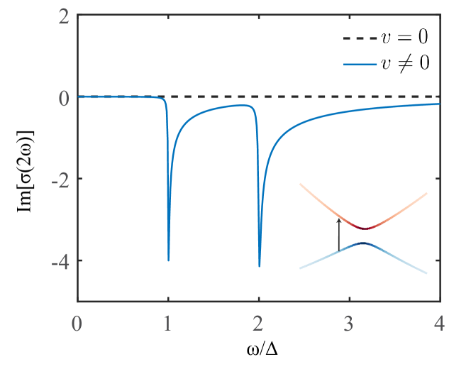
Figure 2: The second harmonic optical absorptions characterized by $\text{Im}[\sigma(2\omega)]$ (in units of $\frac{\tilde{\beta}e^{3}}{2\omega^{2}}$) versus the photon frequency $\omega$, where $\gamma/\Delta=0.01$. The blue and back dashed lines respectively represent the case with CDW motion ($v\neq 0$) and without CDW motion ($v=0$). The inset schematically shows the optical excitation processes of the CDW folded bands in the comoving frame.

Inserting the Hamiltonian $H_{0}(\tilde{k}_{x})$ into the formula of nonlinear optical responses [19] (see SM VI for details), we find that the second-order nonlinear optical conductivity is given by

$$\sigma(2\omega)=\frac{\tilde{\beta}e^{3}}{2\omega^{2}}[2F(\frac{\omega+i\gamma}{\Delta})+F(\frac{2\omega+i\gamma}{\Delta})].$$ (13)

Here, $\omega$ is the photon frequency, $\gamma$ is a small damping parameter, the function $F(a)=\frac{1}{2\pi}[\frac{\pi}{a}+\frac{8}{a\sqrt{a^{2}-4}}(\text{arctanh}(\frac{a}{\sqrt{a^{2}-4}})-\text{arctanh}(\frac{a-2}{\sqrt{a^{2}-4}}))]$, and $F(\frac{\omega+i\gamma}{\Delta})$, $F(\frac{2\omega+i\gamma}{\Delta})$ arise from one-photon and two-photon processes, respectively.

The imaginary part of $\sigma(2\omega)$ representing the second harmonic absorption is plotted in Fig. 2. Note that the real part of $\sigma(2\omega)$ is directly related to $\text{Im}[\sigma(2\omega)]$ according to the Kramers–Kronig relations [20]. The one-photon and two-photon absorption peaks near $\omega=2\Delta$ and $\omega=\Delta$ can be clearly seen. It is worth noting that $\sigma(2\omega)\propto\tilde{\beta}\propto\lambda mv$, while $\tilde{\beta}$ arises from the cubic term in Eq. (10) induced by the additional quartic term in the lab frame. Moreover, as expected, the second-order nonreciprocal nonlinear responses are finite only when the CDW states are moving, i.e. $v\neq 0$ so that $\tilde{\beta}\neq 0$. Therefore, we have explicitly demonstrated the nonreciprocal nonlinear responses in the moving CDW states through the Galilean transformation.

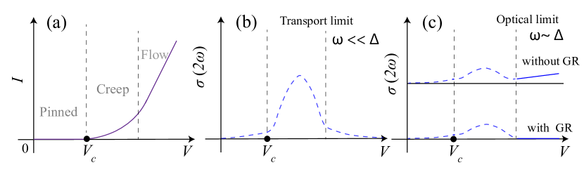
Figure 3: Schematics of nonlinear responses in moving CDW states. (a) Nonlinear voltage ($V$)- current ($I$) relation to highlight the pinned, creep, and flow region respectively. (b) and (c) schematically depict second-order nonlinear response characterized by $\sigma(2\omega)$ under the electric field in the transport limit ($\omega\ll\Delta$) and the optical limit ($\omega\sim\Delta$). The $\sigma(2\omega)$ of the flow region in the optical limit with and without Galilean relativity (GR) are highlighted as solid blue lines, where our theory applies.

It is important to note that with an external excitation at optical frequencies above the CDW energy gap, the quasi-particle effects that we have discussed are dominant. It should be distinguished from the transport region, where the interaction between impurities and collective modes of the CDW should dominate finite frequency responses [12, 11]. As shown in Fig. 3(a), in general, the current-driven CDW states exhibit three distinct regions: the pinned, creep, and flow regions according to the strength of the electric field. The pinned region may exhibit nonlinear responses due to the distortion of the CDW, while the nonlinear responses are expected to peak around the creep region where the depinning motion of CDW is strongest. Our speculation for the nonlinear responses in the transport region ($\omega\ll\Delta$) is shown in Fig. 3(b), where the nonlinear responses mostly stem from the creep motion of the sliding density wave. In the optical limit ($\omega\sim\Delta$), the quasiparticle effects would be more crucial, which fits our interest in this work. In this case, our results imply that the second-order nonlinear conductivity within the flow region linearly increases with the current in the case without emergent Galilean relativity [see the solid blue lines in Fig. 3(c)].

Conclusions and Discussions.— In summary, we have demonstrated the nonreciprocal nonlinear responses in a nonequilibrium system with time-dependent states—moving CDW states through Galilean transformation. Our work not only opens a new avenue in studying nonreciprocal nonlinear responses in nonequilibrium systems but also introduces a new technique Galilean transformation in resolving finite frequency responses of nonequilibrium steady states. Looking ahead, we encourage experimentalists to revisit the quasi-1D CDW materials such as TaS₃, NbSe₃, etc. [12], and explore their nonreciprocal nonlinear optical responses above the gap using advanced terahertz light measurements. A comparative analysis of experimental results with our theoretical insights would be intriguing. Furthermore, we note that the nonreciprocal nonlinear responses would also appear in some other current-driven systems, such as superconductors [21, 22, 23], Weyl materials [24]. However, it is worth pointing out that there is no clear intrinsic time dependence in the lab frame for these systems, which is in contrast with the moving CDW states. Nevertheless, it would be interesting to revisit the nonlinear nonreciprocal responses in current-driven superconductors or topological materials in the comoving frame with our theoretical framework

Y.M.X. acknowledges financial support from the RIKEN Special Postdoctoral Researcher(SPDR) Program. H.I. and N.N. were supported by JSTCREST Grants No.JMPJCR1874.

I Galilean transformation on the field operator

The simplest Lagrangian we are dealing with in this work carries the following form:

$$\mathcal{L}=i\psi^{\dagger}\partial_{t}\psi-\frac{1}{2m}\partial_{i}\psi^{\dagger}\partial_{i}\psi-\psi^{\dagger}V(x,t)\psi.$$ (S1)

Let us perform the Galilean transformation: $x^{\prime}=x-vt$, $t^{\prime}=t$, $\frac{\partial}{\partial t}=\frac{\partial}{\partial t^{\prime}}+\frac{\partial x^{\prime}}{\partial t}\frac{\partial}{\partial x^{\prime}}=\frac{\partial}{\partial t^{\prime}}-v\frac{\partial}{\partial x^{\prime}}$, $\frac{\partial}{\partial x}=\frac{\partial}{\partial x^{\prime}}$. To compensate for the coordinate changes, the field operator should also been transformed

$$\psi=e^{i\eta(x^{\prime},t^{\prime})}\psi^{\prime}.$$ (S2)

After the transformation, the Lagrangian becomes

$$\mathcal{L^{\prime}} =i\psi^{\prime\dagger}\partial_{t^{\prime}}\psi^{\prime}-[\partial_{t^{\prime}}\eta-v\partial_{x^{\prime}}\eta+\frac{1}{2m}(\partial_{x^{\prime}}\eta)^{2}]\psi^{\prime\dagger}\psi^{\prime}$$ (S3)

$$-iv\psi^{\prime\dagger}\partial_{x^{\prime}}\psi^{\prime}-\frac{i}{2m}(\partial_{x^{\prime}}\eta)[(\partial_{x^{\prime}}\psi^{\dagger})\psi^{\prime}-\psi^{\dagger}\partial_{x^{\prime}}\psi]$$

$$-\frac{1}{2m}\partial_{x^{\prime}}\psi^{\prime\dagger}\partial_{x^{\prime}}\psi^{\prime}-\psi^{\prime\dagger}V^{\prime}(x^{\prime},t^{\prime})\psi^{\prime}.$$

To cancel the term in $\psi^{\prime\dagger}\partial_{x^{\prime}}\psi^{\prime}$,

$$-iv+\frac{i}{m}\partial_{x^{\prime}}\eta=0.$$ (S4)

Then it requires

$$\partial_{x^{\prime}}\eta=mv$$ (S5)

We can further fix the form of $\eta$ by considering the system is Galilean invariant in the case without spatial dependent potential $V^{\prime}(x^{\prime},t^{\prime})=V(x,t)=0$. In this case, the Lagrangian would exhibit the same form in the lab frame and moving frame if

$$\partial_{t^{\prime}}\eta-v\partial_{x^{\prime}}\eta+\frac{1}{2m}(\partial_{x^{\prime}}\eta)^{2}=0.$$ (S6)

Now we obtain the phase factor on the field operator under Galilean transformation is given by

$$\eta=mvx^{\prime}+\frac{1}{2}mv^{2}t^{\prime}=mvx-\frac{1}{2}mv^{2}t.$$ (S7)

In the case of moving CDW, the potential $V(x,t)=V(x-vt)$ is mapped to $V(x^{\prime})$ in the comoving frame after the Galilean transformation.

In a broader context, we aim to execute a gauge transformation, denoted as $\psi=e^{i\eta(x,t)}\psi^{\prime}$, to convert a time-dependent problem into a time-independent one. Since this transformation merely alters the phase of the field operator, the physical outcomes remain unaffected by the specific choice of $\eta(x,t)$. In essence, we can endeavor to apply an appropriate gauge transformation to a more generic Lagrangian, thereby transitioning from a time-dependent scenario to a stationary one.

II Transformation of electromagnetic fields and current from special relativity

To make the work self-content, let us summarize the transformation of electromagnetic fields and current from special relativity here [18], which has been used in the main text in understanding the optical responses of the moving CDW states.

The antisymmetric field-strength tensor is

$$F^{\alpha\beta}=\begin{pmatrix}0&-E_{x}&-E_{y}&-E_{z}\\ E_{x}&0&-B_{z}&B_{y}\\ E_{y}&B_{z}&0&-B_{x}\\ E_{z}&-B_{y}&B_{x}&0\end{pmatrix}$$ (S8)

Here, $E_{i}$ and $B_{i}$ denote the electric and magnetic field, respectively, along $i$-direction. Under the Lorentz transformation,

$$F^{\prime\alpha\beta}=\frac{\partial x^{\prime\alpha}}{\partial x^{\gamma}}\frac{\partial x^{\prime\beta}}{\partial x^{\delta}}F^{\gamma\delta}.$$ (S9)

where the four vector $x^{\alpha}=(ct,x,y,z)$, and $c$ is the speed of light. The Galilean transformation is recovered by taking the small velocity limit $v\ll c$. Let us simply take the transformation along $x$-direction, then the boost matrix is simplified as

$$A=\begin{pmatrix}\gamma&-\frac{v}{c}\gamma&0&0\\ -\frac{v}{c}\gamma&\gamma&0&0\\ 0&0&1&0\\ 0&0&0&1\end{pmatrix}.$$ (S10)

Here, $\gamma=\sqrt{1-v^{2}/c^{2}}$ is the Lorentz factor. In this case, the Lorentz transformation of the field-strength tensor can be represented in a matrix form:

$$F^{\prime}=AFA^{T}.$$ (S11)

According to this transformation, in the low-velocity limit, the electromagnetic fields transform can be deduced as

$$\bm{E^{\prime}}=\bm{E}+\frac{\bm{v}}{c}\times\bm{B}$$ (S12)

$$\bm{B^{\prime}}=\bm{B}-\frac{\bm{v}}{c}\times\bm{E}$$ (S13)

The four vector $J^{\alpha}=(c\rho,\bm{J})$. Under the Lorentz transformation,

$$J^{\prime\alpha}=\frac{\partial x^{\prime\alpha}}{\partial x^{\beta}}J^{\beta}$$ (S14)

or in the matrix representation

$$J^{\prime}=AJ.$$ (S15)

Then the charge and current transform as.

$$\rho^{\prime}=\rho-\frac{\bm{v}\cdot\bm{J}}{c^{2}}\approx\rho,\ \bm{J^{\prime}}=\bm{J}-\bm{v}\rho$$ (S16)

For the electrons, the Galilean transformation of current is thus given by

$$\bm{J^{\prime}}=\bm{J}+Ne\bm{v}.$$ (S17)

Here, $N$ is the number of eletrons.

III The current relation between the lab and comoving frame under the Galilean transformation

III.1 The current relation under the Galilean transformation up to quartic term in real-space

To derive the current operator, we consider the Lagrangian in the presence electromagnetic fields as

$$\mathcal{L}[\mathcal{A}_{i}] =i\psi^{\dagger}\partial_{t}\psi-\frac{1}{2m}(\partial_{i}\psi^{\dagger}-ieA_{i}\psi^{\dagger})(\partial_{i}+ieA_{i})\psi$$ (S18)

$$-\psi^{\dagger}V(x-vt)\psi+\delta\mathcal{L}[\mathcal{A}_{i}],$$

$$\delta\mathcal{L} =-\lambda(\partial_{i}-ieA_{i})^{2}\psi^{\dagger}(\partial_{i}+ieA_{i})^{2}\psi.$$ (S19)

Here, we set $i=x$ without loss of generality. To make the derivation more general, the quartic term $\delta\mathcal{L}$ is also included. As we would show later, the quartic term plays a crucial role in affecting the nonlinear nonreciprocal responses.

The current operator is given by

$$\hat{j}_{i} =\frac{\partial\mathcal{L}}{\partial A_{i}}|_{A_{i}=0}=\frac{ie}{2m}(\psi^{\dagger}\partial_{i}\psi-\partial_{i}\psi^{\dagger}\psi)+\delta\hat{j}_{i},$$ (S20)

$$\delta\hat{j}_{i} =2ie\lambda(\partial_{i}\psi^{\dagger}\partial_{i}^{2}\psi-\partial_{i}^{2}\psi^{\dagger}\partial_{i}\psi).$$ (S21)

Here, $\delta\hat{j}_{i}$ arises from the quartic term.

To obtain the current operator in the comoving frame, we can first write down the Lagrangian in the comoving frame as

$$\mathcal{L^{\prime}}=i\psi^{\prime\dagger}\partial_{t^{\prime}}\psi^{\prime}-\frac{1}{2m}\partial_{x^{\prime}}\psi^{\dagger}\partial_{x^{\prime}}\psi-\psi^{\prime\dagger}V(x^{\prime})\psi^{\prime}+\delta\mathcal{L^{\prime}}.$$ (S22)

Here,

$$\delta\mathcal{L}^{\prime} =-\lambda e^{i\eta(x^{\prime},t^{\prime})}\psi^{\prime\dagger}\partial_{x^{\prime}}^{4}[e^{-i\eta(x^{\prime},t^{\prime})}\psi^{\prime}]$$ (S23)

$$=-\lambda m^{4}v^{4}\psi^{\prime\dagger}\psi^{\prime}+4i\lambda m^{3}v^{3}\psi^{\prime\dagger}\partial_{x^{\prime}}\psi^{\prime}+6\lambda m^{2}v^{2}\psi^{\prime\dagger}\partial_{x^{\prime}}^{2}\psi^{\prime}$$

$$-4i\lambda mv\psi^{\prime\dagger}\partial_{x^{\prime}}^{3}\psi^{\prime}-\lambda\psi^{\prime\dagger}\partial_{x^{\prime}}^{4}\psi^{\prime}.$$

Similarly, the current-density operator in the comoving frame given by the Lagrangian is

$$\hat{j}_{x}^{\prime} =\frac{ie}{2m}(\psi^{\prime\dagger}\partial_{x^{\prime}}\psi^{\prime}-\partial_{x^{\prime}}\psi^{\prime\dagger}\psi^{\prime})+4e\lambda m^{3}v^{3}\psi^{\prime\dagger}\psi^{\prime}$$ (S24)

$$+6ie\lambda m^{2}v^{2}(\psi^{\prime\dagger}\partial_{x^{\prime}}\psi^{\prime}-\partial_{x^{\prime}}\psi^{\prime\dagger}\psi^{\prime})+12\lambda emv\psi^{\prime\dagger}\partial_{x^{\prime}}^{2}\psi^{\prime}$$

$$+2ie\lambda(\partial_{x^{\prime}}\psi^{\dagger}\partial_{x^{\prime}}^{2}\psi^{\prime}-\partial_{x^{\prime}}^{2}\psi^{\prime\dagger}\partial_{x^{\prime}}\psi^{\prime}).$$

To see the relation between $\hat{j}_{x}^{\prime}$ and $\hat{j}_{x}$, we can express $\hat{j}_{x}$ in the comoving frame. Using $\psi=e^{i\eta}\psi^{\prime}$ and Eq. (S21) and (S21), we deduce that

$$\hat{j}_{x} =\frac{ie}{2m}(\psi^{\prime\dagger}\partial^{\prime}_{i}\psi-\partial^{\prime}_{i}\psi^{\prime\dagger}\psi^{\prime})-ev\psi^{\prime\dagger}\psi^{\prime}+4e\lambda m^{3}v^{3}\psi^{\prime\dagger}\psi^{\prime}$$

$$+6ie\lambda m^{2}v^{2}(\psi^{\prime\dagger}\partial_{i}\psi^{\prime}-\partial_{i}\psi^{\prime\dagger}\psi^{\prime})+12e\lambda mev\psi^{\prime\dagger}\partial_{i}^{2}\psi^{\prime}$$

$$+2ie\lambda(\partial_{i}\psi^{\prime\dagger}\partial_{i}^{2}\psi^{\prime}-\partial_{i}^{2}\psi^{\prime\dagger}\partial_{i}\psi^{\prime}).$$

By comparing Eqs. (S24) and (LABEL:eq_s25a), we find

$$\hat{j}_{x}^{\prime}=\hat{j}_{x}+ev\psi^{\prime\dagger}\psi^{\prime}$$ (S26)

Let us denote the ground state in the lab frame as

$$\ket{G}=\Pi_{j=1}^{N}\int dx\psi^{\dagger}_{j}(x,t)\ket{0}$$ (S27)

Then, the ground state in the comoving frame reads

$$\ket{G^{\prime}} =\Pi_{j=1}^{N}\int dx^{\prime}\psi^{\prime\dagger}_{j}(x^{\prime},t^{\prime})\ket{0}$$ (S28)

$$=\Pi_{j=1}^{N}\int dxe^{i\eta(x,t)}\psi^{\dagger}_{j}(x,t)\ket{0}$$

It can be seen that

$$\braket{G^{\prime}}{\hat{j}_{x}^{\prime}}{G^{\prime}} =\braket{G}{e^{-i\eta}\hat{j}_{x}e^{i\eta}}{G}+ev\braket{G^{\prime}}{\psi^{\prime\dagger}\psi}{G^{\prime}}$$ (S29)

$$=\braket{G}{\hat{j}_{x}}{G}+evN.$$

Therefore, we have demonstrated the current relation under Galilean transformation still holds for the Lagrangian even with quartic term:

$$J_{x}^{\prime}(t^{\prime})=J_{x}(t)+evN.$$ (S30)

Here, we define $J^{\prime}_{x}(t^{\prime})=\braket{G^{\prime}}{\hat{j}_{x}^{\prime}}{G^{\prime}}$, and $J_{x}(t)=\braket{G}{\hat{j}_{x}}{G}$. Next, let us try to argue the above relation still holds for a generic energy dispersion through the Galilean transformation in the momentum space.

III.2 The current relation with a generic dispersion through the Galilean transformation in the momentum space

The Lagrangian of the comoving frame in the momentum space reads

$$\mathcal{L^{\prime}}=i\sum_{k^{\prime}}\psi^{\prime\dagger}_{k^{\prime}}\partial_{t^{\prime}}\psi_{k^{\prime}}-\epsilon(k^{\prime})\psi^{\prime\dagger}_{k^{\prime}}\psi_{k^{\prime}}^{\prime}+\mathcal{L}_{\text{CDW}}$$ (S31)

As the CDW is a potential term, it would affect the ground states but not affect the current operator. So we next derive the current operator using the Lagrangian

$$\mathcal{L}^{\prime}_{0}=i\sum_{k^{\prime}}\psi^{\prime\dagger}_{k^{\prime}}\partial_{t^{\prime}}\psi_{k^{\prime}}-\epsilon(k^{\prime})\psi^{\prime\dagger}_{k^{\prime}}\psi_{k^{\prime}}^{\prime}.$$ (S32)

Then the current operator in the comoving frame reads

$$\hat{J}^{\prime}=e\sum_{k^{\prime}}\frac{\partial\epsilon(k^{\prime})}{\partial_{k^{\prime}}}\psi^{\prime\dagger}_{k^{\prime}}\psi^{\prime}_{k^{\prime}}.$$ (S33)

The field operators in the two frames are related through $\psi_{k}(t)=\int dxe^{-ikx}\psi(x,t)=e^{-i(kv-\frac{1}{2}mv^{2})t^{\prime}}\psi^{\prime}_{k-mv}(t^{\prime})$, or equivalently

$$\psi^{\prime}_{k^{\prime}}(t^{\prime})=e^{i(k^{\prime}v+\frac{1}{2}mv^{2})t}\psi_{k^{\prime}+mv}(t).$$ (S34)

Let us define $k=k^{\prime}+mv$, and after this Galilean transformation in the momentum space, we find that the Lagrangian in the lab frame is given by

$$\mathcal{L}_{0}=i\sum_{k}\psi^{\dagger}_{k}\partial_{t}\psi_{k}-[\epsilon(k-mv)+kv-\frac{1}{2}mv^{2}]\psi^{\dagger}_{k}\psi_{k}.$$ (S35)

The current operator in the lab frame is given by

$$\hat{J}=e\sum_{k}(\frac{\epsilon(k-mv)}{\partial k}+v)\psi_{k}^{\dagger}\psi_{k}.$$ (S36)

Let us denote the ground states in the presence of external fields and CDW as $\ket{G^{\prime}}$ $(\ket{G})$ in the comoving (lab) frame. Then the current in comoving frame is

$$J^{\prime}(t)=e\sum_{k^{\prime}}\frac{\partial\epsilon(k^{\prime})}{\partial_{k^{\prime}}}\braket{G^{\prime}}{\psi^{\prime\dagger}_{k^{\prime}}\psi^{\prime}_{k^{\prime}}}{G^{\prime}}$$ (S37)

while the current in the lab frame is

$$J^{\prime}(t) =e\sum_{k}(\frac{\epsilon(k-mv)}{\partial k}+v)\braket{G}{\psi_{k}^{\dagger}\psi_{k}}{G}$$ (S38)

Here, we have considered that the number of electrons does not change in the ground states upon Galilean transformation. It can be seen that the group velocity of each electron is uniformly shifted by $v$. As a result, we finally obtain the relation:

$$J^{\prime}(t)=J(t)+evN$$ (S39)

where the total number of electrons $N=\sum_{k^{\prime}}\braket{G^{\prime}}{\psi^{\dagger}_{k^{\prime}}\psi_{k^{\prime}}}{G^{\prime}}$.

IV Optical responses formalism

In this section, we present the detailed derivations of the linear and second-harmonic optical conductivity. Note that to make the unit of conductance clear, we would keep the $\hbar$ below (which was set to be 1 in the main text). The linear optical conductivity is given by the bubble diagram [19],

$$\sigma^{\mu\alpha}(\omega;\omega)=\frac{ie^{2}}{\hbar\omega}\sum_{a\neq b}\int\frac{d^{d}\bm{k}}{(2\pi)^{d}}\frac{f_{ab}v_{ab}^{\alpha}v_{ba}^{\mu}}{\omega-\epsilon_{ba}}.$$ (S40)

where $d$ is the spatial dimension, the sandwich of velocity operator between interband $v_{ab}^{\alpha}=\braket{a}{\partial_{k_{\alpha}}H(\bm{k})}{b}$, the energy and Fermi distribution difference between the band $\epsilon_{a}$ and $\epsilon_{b}$ are represented as $\epsilon_{ba}=\epsilon_{b}-\epsilon_{a}$, $f_{ab}=f(\epsilon_{a})-f(\epsilon_{b})$, respectively.

The Hamiltonian we are dealing with generally takes the following form:

$$H(\bm{k})=\begin{pmatrix}\xi_{+}(\bm{k})&\Delta\\ \Delta&\xi_{-}(\bm{k})\end{pmatrix}.$$ (S41)

It is easy to show that the eigenvalues of $H^{\prime}(\bm{k})$ is given by $E_{\pm}=\frac{\xi_{+}(\bm{k})+\xi_{-}(\bm{k})}{2}\pm\epsilon(\bm{k})$ with $\epsilon(\bm{k})=\sqrt{\frac{(\xi_{+}(\bm{k})-\xi_{-}(\bm{k}))^{2}}{4}+\Delta^{2}}$, the eigenfunctions are $\ket{E_{+}}=(\cos\frac{\theta_{\bm{k}}}{2},\sin\frac{\theta_{\bm{k}}}{2})^{T}$, and $\ket{E_{-}}=(-\sin\frac{\theta_{\bm{k}}}{2},\cos\frac{\theta_{\bm{k}}}{2})^{T}$ with $\sin\theta_{\bm{k}}=\Delta/\epsilon(\bm{k})$. As a result, $v^{x}_{+-}(\bm{k})=\braket{E_{+}}{\partial_{k_{x}}H}{E_{-}}=\frac{1}{2}\sin\theta_{\bm{k}}(\partial_{k_{x}}\xi_{-}-\partial_{k_{x}}\xi_{+})=\frac{\Delta}{2\epsilon(\bm{k})}(\partial_{k_{x}}\xi_{-}-\partial_{k_{x}}\xi_{+}).$

In the main text, the focus is the nonlinear responses. Here, let us try to show that the linear optical response also satisfies Galilean relativity. For simplicity, we set $\lambda=0$ as the finite linear responses do not have to involve the quartic term. In this case, in the comoving frame, the Hamiltonian reads,

$$H^{\prime}(k)=\begin{pmatrix}v_{F}k_{x}&\Delta\\ \Delta&-v_{F}k_{x}\end{pmatrix}$$ (S42)

In contrast, the Hamiltonian in the lab frame is written as

$$H(k,t)=\begin{pmatrix}v_{F+}k_{x}&\Delta e^{-i\omega_{0}t}\\ \Delta e^{i\omega_{0}t}&-v_{F-}k_{x}\end{pmatrix}.$$ (S43)

In general, it is difficult to obtain the optical conductivity in the lab frame due to the time dependence. But in the low drift velocity limit, $\hbar\omega_{0}\approx\frac{v}{v_{F}}E_{F}\ll\Delta$, we may replace the time-dependent phase change $\omega_{0}t$ with a constant phase to study the optical responses using

$$H_{0}(k)=\begin{pmatrix}v_{F+}k&\Delta\\ \Delta&-v_{F-}k\end{pmatrix}.$$ (S44)

Note that a constant phase on $\Delta$ can always be gauged out. It is worth noting that in the small drift velocity approximation, inversion and time-reversal symmetries are still broken in the lab frame, different from the case of the co-moving frame.

Now let us replace the Hamiltnoian $H(\bm{k})$ with $H_{0}(\bm{k})$. Note that the linear optical responses are dominant by the linearized Hamiltonian, while higher-order terms can be neglected. It can be seen that

$$v_{+-}^{x}=-\frac{\Delta(v_{F+}+v_{F-})}{\omega}.$$ (S45)

The linear optical conductivity at zero-temperature limit given by the two-band model $H_{0}(\bm{k})$ is

$$\sigma_{R}^{xx}(\omega;\omega) =\frac{e^{2}}{\hbar\omega}\sum_{a\neq b}\int[d\bm{k}]f_{ab}v_{ab}^{x}v_{ba}^{x}\delta(\omega-E_{ba})$$ (S46)

$$=\frac{e^{2}}{\hbar\omega}\int\frac{dk_{x}}{2\pi}(f_{-}-f_{+})|v^{x}_{+-}|^{2}\delta(\omega-2\epsilon(k_{x}))$$

$$=\frac{e^{2}}{\hbar\omega}\frac{|v_{+-}^{x}(k_{x0})|^{2}}{|\partial_{k_{x0}}\epsilon(k_{x0})|}\text{with }2\epsilon(k_{x0})=\omega.$$

Inserting Eq. (S45) and using $|\partial_{k_{x0}}\epsilon(k_{x0})|^{-1}=\frac{\omega}{\sqrt{\omega^{2}/4-\Delta^{2}}(v_{F+}+v_{F-})}$, we find that

$$\sigma_{R}^{xx}(\omega;\omega)=\frac{4e^{2}\Delta^{2}(v_{F,+}+v_{F,-})}{\hbar\omega^{2}\sqrt{\omega^{2}-4\Delta^{2}}}.$$ (S47)

For the Hamiltonian $H^{\prime}(k)$ in the comoving frame, we can simply replace $v_{F\pm}$ as $v_{F}$ in the optical conductivity. It can be seen that the linear optical conductivity is the same in the comoving frame and lab frame, being consistent with our argument from Galilean relativity.

Next, we present the formulism for the second-order optical responses. The optical conductivity for the second-harmonic generation can be rewritten as [19]

$$\sigma^{\mu\alpha\beta}(2\omega;\omega,\omega) =\sigma_{\text{I}}^{\mu\alpha\beta}(2\omega;\omega,\omega)+\sigma_{\text{II}}^{\mu\alpha\beta}(2\omega;\omega,\omega),$$ (S48)

$$\sigma_{\text{I}}^{\mu\alpha\beta} =-\frac{e^{3}}{2\hbar^{2}\omega^{2}}\sum_{a\neq b}\int[d\bm{k}]f_{ab}\frac{v_{ab}^{\alpha}v_{ba}^{\mu\beta}+v_{ab}^{\beta}v_{ba}^{\mu\alpha}}{\omega-\epsilon_{ab}}$$ (S49)

$$+f_{ab}\frac{v_{ab}^{\alpha\beta}v_{ba}^{\mu}}{2\omega-\epsilon_{ab}},$$

$$\sigma_{\text{II}}^{\mu\alpha\beta} =-\frac{e^{3}}{2\hbar^{2}\omega^{2}}\sum_{a\neq b\neq c}\int[d\bm{k}]\frac{(v_{ab}^{\alpha}v_{bc}^{\beta}+v_{ab}^{\beta}v_{bc}^{\alpha})v_{ca}^{\mu}}{\epsilon_{ab}+\epsilon_{cb}}($$ (S50)

$$\frac{2f_{ac}}{2\omega-\epsilon_{ca}}+\frac{f_{cb}}{\omega-\epsilon_{cb}}+\frac{f_{ba}}{\omega-\epsilon_{ba}}).$$

where $2\omega$ and $\omega$ in Eqs. (S49) and (S50) characterize the contributions from two-photon and one-photon processes, respectively. The second-order derivation of Hamiltonian $v_{ba}^{\mu\beta}=\braket{b\bm{k}}{\partial_{k_{\mu}}\partial_{k_{\beta}}H(\bm{k})}{a\bm{k}}$. The contribution that involves two (three) different bands is labeled as $\sigma_{\text{I}}^{\mu\alpha\beta}$ ($\sigma_{\text{II}}^{\mu\alpha\beta}$), respectively. For the compact of notations, in the following, we label the second-harmonic generation response tensor $\sigma^{xxx}(2\omega;\omega,\omega)\equiv\sigma^{xxx}(2\omega)$.

V Nonlinear transport induced by the quartic term in the lab frame

For a current-driven system, the time-reversal and inversion symmetry are broken so one may expect non-reciprocal nonlinear transport. But as we discussed Galilean relativity would constrain the nonlinear responses. If we break Galilean relativity, such as with some higher momentum terms, the non-reciprocal nonlinear responses could be back. As an illustration, we now present the study of nonlinear transport with a more generic band dispersion:

$$\epsilon(k_{x})=\frac{k_{x}^{2}}{2m}+\lambda k_{x}^{4},$$ (S51)

where the higher-order term (the second term) breaks the Galilean relativity. Note that our discussion in this section does not involve the CDW order, but focuses on the nonlinear transport given by the simple band $\epsilon(k_{x})$. In the below, we show that the nonlinear transport is only contributed by this higher-order term using the Boltzmann transport theory.

As we mentioned in the main text, to extract the second-harmonic nonlinear responses, the experiment can replace the current with a DC one plus a small AC component: $J(t)=J_{0}+J_{ac}\cos(\omega t)$. The DC component is to break the inversion symmetry. It would be expected that the cubic nonlinear responses $V_{3}=R_{3}J^{3}$ ($V_{3}$ is the voltage, $R_{3}$ is the resistance) would give rise to a $2\omega$-signal: $V_{2\omega}=3R_{3}J_{0}J_{ac}^{2}$. So next, we would evaluate the nonlinear conductivity $\sigma(2\omega)$ for the third-order nonlinear responses.

The transport current in the semi-classical approach is given by

$$\bm{j}=-e\sum_{n}\int\frac{d\bm{k}}{(2\pi)^{d}}\sum_{n}f_{n}\bm{v}_{n},$$ (S52)

Here, $n$ is the band index, $f$ is the Fermi-distribution function. The group velocity is given by

$$v_{n}(\bm{k})=\frac{1}{\hbar}\frac{\partial\epsilon_{n}}{\partial\bm{k}}-\frac{e}{\hbar}\bm{E}\times\bm{\Omega}_{n},$$ (S53)

where $\bm{E}$ is the electric field, $\bm{\Omega}_{n}$ is the Berry curvature of the $n$-th band. For our single-band consideration ($n=1$), the group velocity is reduced to $\bm{v}_{n}(\bm{k})=\frac{1}{\hbar}\frac{\partial\epsilon_{n}}{\partial\bm{k}}$.

We can expand the Fermi-distribution function order by order in terms of $\bm{E}$. To obtain the third-order nonlinear responses, we expand the current up to the third-order:

$$\bm{j}^{(1)} =-e\int\frac{d\bm{k}}{(2\pi)^{d}}\sum_{n}f_{n}^{(1)}\bm{v}_{n},$$ (S54)

$$\bm{j}^{(2)} =-e\int\frac{d\bm{k}}{(2\pi)^{d}}\sum_{n}f_{n}^{(2)}\bm{v}_{n},$$ (S55)

$$\bm{j}^{(3)} =-e\int\frac{d\bm{k}}{(2\pi)^{d}}\sum_{n}f_{n}^{(3)}\bm{v}_{n}.$$ (S56)

The Fermi-distribution correction can be determined through the Boltzmann equation:

$$\partial_{t}f-\frac{e\bm{E}(t)}{\hbar}\cdot\nabla_{\bm{k}}f+\bm{v}\nabla_{\bm{r}}f=I(f).$$ (S57)

Here, $I(f)$ is the collision function, $\bm{r}$ is the position vector. To drive the DC plus AC current, the applied electric field can be denoted as

$$\bm{E}(t)=\bm{E}_{0}+\text{Re}[\bm{E}e^{i\omega t}].$$ (S58)

Using the scattering time approximation, $I(f)=-\frac{f-f_{0}}{\tau}$, and assume $f$ is uniform, it yields

$$\partial_{t}f-\frac{e\bm{E}(t)}{\hbar}\cdot\nabla_{\bm{k}}f=-\frac{f-f_{0}}{\tau}.$$ (S59)

Let us expand, $f(\bm{k},t)=f_{0}+f^{(1)}(\bm{k},t)+f^{(2)}(\bm{k},t)+f^{(3)}(\bm{k},t)$, and solve the equation iteratively. Here, the order is characterized by the electric field $\bm{E}$. The Boltzmann equation for the first-order response is then given by

$$\partial_{t}f^{(1)}-\frac{e\bm{E}(t)}{\hbar}\cdot\nabla_{\bm{k}}f^{(0)}=-\frac{f^{(1)}}{\tau}.$$ (S60)

Perform Fourier transformation on both sides with $f^{(1)}=\sum_{p}f^{(1)}_{p}e^{ip\omega t}$ ($p$ are integers), we find

$$f_{n}^{(1)}(t) =\frac{eE_{0a}\tau}{\hbar}\partial_{k_{a}}f_{n}^{(0)}+\frac{e}{2\hbar}[\frac{E_{a}\partial_{k_{a}}f_{n}^{(0)}}{i\omega+\tau^{-1}}e^{i\omega t}$$ (S61)

$$+\frac{E_{a}\partial_{k_{a}}f_{n}^{(0)}}{-i\omega+\tau^{-1}}e^{-i\omega t}].$$

Similarly, the Boltzmann equation to the higher order reads

$$\partial_{t}f^{(k+1)}-\frac{eE_{a}(t)}{\hbar}\partial_{k_{a}}f^{(n)}=-\frac{f^{(k+1)}}{\tau}.$$ (S62)

In the frequency space, we obtain

$$f_{n}^{(k+1)}(m\omega)=\frac{eE_{a}(m_{1}\omega)}{\hbar(im\omega+\tau^{-1})}\partial_{k_{a}}f_{n}^{(k)}(m_{2}\omega)\delta_{m_{1}+m_{2},m}.$$ (S63)

Here, $m$ and $m_{i}$ are integers. Inserting Eq. (S61) into the iteration equation Eq. (S63), we obtain the second-order correction of Fermi distribution

$$f_{n}^{(2)}=f_{n}^{(2)}(0)+\sum_{\pm}f_{n}^{(2)}(\pm\omega)e^{\pm i\omega t}+f_{n}^{(2)}(\pm 2\omega)e^{\pm i2\omega t}.$$ (S64)

Here,

$$f_{n}^{(2)}(0) =\frac{\tau^{2}e^{2}E_{0a}E_{0b}}{\hbar^{2}}\partial_{k_{a}}\partial_{k_{b}}f_{n}^{(0)},$$ (S65)

$$f_{n}^{(2)}(\pm\omega) =\frac{\tau e^{2}E_{a}E_{0b}\partial_{k_{a}}\partial_{k_{b}}f_{n}^{(0)}}{2\hbar^{2}(\pm i\omega+\tau^{-1})}+\frac{e^{2}E_{0a}E_{b}\partial_{k_{a}}\partial_{k_{b}}f_{n}^{(0)}}{2\hbar^{2}(\pm i\omega+\tau^{-1})^{2}},$$

$$f_{n}^{(2)}(\pm 2\omega) =\frac{e^{2}}{4\hbar^{2}}\frac{E_{a}E_{b}\partial k_{a}\partial k_{b}f_{n}^{(0)}}{(\pm 2i\omega+\tau^{-1})(\pm i\omega+\tau^{-1})}.$$ (S67)

Inserting $f_{n}^{(2)}$ into the iteration equation Eq. (S63) again, we find the third-order correction on the Fermi-distribution function reads

$$f_{n}^{(3)}= f_{n}^{(3)}(0)+\sum_{\pm}f_{n}^{(3)}(\pm\omega)e^{\pm i\omega t}+\sum_{\pm}f_{n}^{(3)}(\pm 2\omega)e^{\pm 2i\omega t}$$ (S68)

$$+\sum_{\pm}f_{n}^{(3)}(\pm 3\omega)e^{\pm 3i\omega t}.$$

The specific form of $2\omega$ component is written as

$$f_{n}^{(3)}(\pm 2\omega)=\frac{eE_{0c}\partial_{k_{c}}f_{n}^{(2)}(2\omega)}{\hbar(2i\omega+\tau^{-1})}+\frac{eE_{c}\partial_{k_{c}}f_{n}^{(2)}(\omega)}{2\hbar(i2\omega+\tau^{-1})},$$

$$=\frac{3e^{3}E_{0a}E_{b}E_{c}\Gamma(\omega,\tau)\partial_{k_{a}}\partial_{k_{b}}\partial_{k_{c}}f_{n}^{(0)}}{4\hbar^{3}}$$ (S69)

where

$$\Gamma(\omega,\tau)=\frac{1}{(2i\omega+\tau^{-1})^{2}(i\omega+\tau^{-1})}+\frac{\tau}{(2i\omega+\tau^{-1})(i\omega+\tau^{-1})}$$

$$+\frac{1}{(2i\omega+\tau^{-1})(i\omega+\tau^{-1})^{2}}.$$ (S70)

Inserting Eq. (S69) back to Eq. (S56) term, the $2\omega$-component of conductivity given by the third-order nonlinear response is

$$\sigma_{abc}^{(3)}(2\omega)=\frac{e^{4}\Gamma(\omega,\tau)}{4\hbar^{3}}\int\frac{d\bm{k}}{(2\pi)^{d}}f_{n}^{(0)}\partial_{k_{a}}\partial_{k_{b}}\partial_{k_{c}}v_{n}(k).$$

Here, we have performed integration by parts to put the Fermi distribution function ahead.

For the dispersion $\epsilon(k_{x})=\frac{k_{x}^{2}}{2m}+\lambda k_{x}^{4}$, the group velocity $v(k_{x})=\frac{k_{x}}{m}+4\lambda k_{x}^{3}$. Then we obtain

$$\sigma_{xxx}^{(3)}(2\omega) =\frac{e^{4}\Gamma(\omega,\tau)}{4\hbar^{3}}\int\frac{dk_{x}}{2\pi}f^{(0)}\partial_{k_{x}}^{3}v(k_{x}),$$ (S72)

$$=\frac{6e^{4}\lambda n\Gamma(\omega,\tau)}{\hbar^{3}}.$$

Here, the electron density $n=\int\frac{dk_{x}}{2\pi}f^{(0)}(\epsilon(k_{x})-\epsilon_{F})$. Interestingly, we can see that the nonlinear transport would be finite only when the higher order term is there ($\lambda\neq 0$).

VI Nonlinear responses induced by the quartic term studied in the comoving frame

In the previous section, we have introduced a quartic term into the Hamiltonian in the lab frame, i.e.,

$$\delta H=\lambda\psi^{\dagger}\partial_{x}^{4}\psi$$ (S73)

It turns out that this term plays a crucial role in affecting the nonlinear transport in the lab. The natural question is how it would modify the nonlinear responses in the comoving frame. Here, the comoving frame is the frame in which the CDW order parameter is static.

To address this question, we can perform the Galilean transformation is

$$\psi=e^{i\eta(x^{\prime},t^{\prime})}\psi^{\prime}$$ (S74)

with $\eta(x^{\prime},t^{\prime})=mvx^{\prime}+\frac{1}{2}mv^{2}t^{\prime}$. Here, we perform such a gauge transformation in order to make the CDW order parameter static. In the comoving frame, the quartic Hamiltonian becomes

$$\delta H =\lambda e^{-i\eta(x^{\prime},t^{\prime})}\psi^{\prime\dagger}\partial_{x^{\prime}}^{4}[e^{i\eta(x^{\prime},t^{\prime})}\psi^{\prime}]$$ (S75)

$$=\lambda m^{4}v^{4}\psi^{\prime\dagger}\psi^{\prime}-4i\lambda m^{3}v^{3}\psi^{\prime\dagger}\partial_{x^{\prime}}\psi^{\prime}-6\lambda m^{2}v^{2}\psi^{\prime\dagger}\partial_{x^{\prime}}^{2}\psi^{\prime}$$

$$+4i\lambda mv\psi^{\prime\dagger}\partial_{x^{\prime}}^{3}\psi^{\prime}+\lambda\psi^{\prime\dagger}\partial_{x^{\prime}}^{4}\psi^{\prime}.$$

It can be seen that there are residual higher order terms in the comoving frame that break the explicit Galilean relativity. Using $\psi^{\prime}_{\tilde{k}_{x}}=\int dx^{\prime}e^{-i\tilde{k}_{x}x^{\prime}}\psi^{\prime}(x^{\prime})$, we find that in the comoving frame, the energy dispersion including both the original quadratic term and the higher order term becomes

$$\epsilon_{k^{\prime}_{x}}=\frac{k_{x}^{\prime 2}}{2m}+4\lambda m^{3}v^{3}k_{x}^{\prime}+6\lambda m^{2}v^{2}k_{x}^{\prime 2}+4\lambda mvk_{x}^{\prime 3}+\lambda k_{x}^{\prime 4}.$$ (S76)

The constant term in Eq. (S75) is dropped, which is simply shifted the chemical potential. Next, let us see how the cubic term in $\epsilon_{k^{\prime}}$ would give rise to the second harmonic generation in the comoving frame.

We expand the states near the Fermi momenta ($k^{\prime}_{x}=\tilde{k}_{x}+sk_{F}$) with $s=\pm$ up to $\tilde{k}_{x}^{2}$ term:

$$\tilde{\epsilon}_{s,\tilde{k}_{x}}\approx(s\tilde{v}_{F}+\delta v_{F})\tilde{k}_{x}+(s\tilde{\beta}+\delta\beta)\tilde{k}_{x}^{2}+s\tilde{\alpha},$$ (S77)

with

$$\tilde{v}_{F} =v_{F}+12\lambda m^{2}v^{2}k_{F}+4\lambda k_{F}^{3},$$ (S78)

$$\delta v_{F} =4\lambda m^{3}v^{3}+12\lambda mvk_{F}^{2},$$ (S79)

$$\tilde{\beta} =12\lambda mvk_{F},$$ (S80)

$$\delta\beta =\frac{1}{2m}+6\lambda m^{2}v^{2}+6\lambda k_{F}^{2},$$ (S81)

$$\tilde{\alpha} =4\lambda mvk_{F}(k_{F}^{2}+m^{2}v^{2})$$ (S82)

Here $\tilde{\beta}$ arises from the cubic term in Eq. (S76) that breaks the inversion symmetry, which would be essential for the second-order nonlinear optical responses as we would see later.

The low-energy Hamiltonian for the CDW state is given by

$$H_{0}(\tilde{k}_{x})=\begin{pmatrix}\tilde{\epsilon}_{+,\tilde{k}_{x}}&\Delta\\ \Delta&\tilde{\epsilon}_{-,\tilde{k}_{x}}\end{pmatrix}$$ (S83)

The focus here would be the nonlinear responses. Still only the two-band process $\sigma_{I}^{\mu\alpha\beta}$ is finite. We assume the higher order term is small so that $\tilde{v}_{F}\gg\delta v_{F},\tilde{\beta},\delta\beta$ so that the eigenstates are approximately given by the lowest order. On the other hand, the interband matrix element for the second-order derivative of Hamiltonian (see Sec. IV) is

$$v^{xx}_{+-}\approx-\tilde{\beta}\sin\theta_{\tilde{k}_{x}}.$$ (S84)

where $\sin\theta_{\tilde{k}_{x}}\approx\frac{\Delta}{\epsilon(\tilde{k}_{x})}$, with $\epsilon(\tilde{k}_{x})=\sqrt{\tilde{v}_{F}^{2}\tilde{k}_{x}^{2}+\Delta^{2}}$. Note that the terms in Eq. (S83) with identity matrix does not contribute as the eigen wavefunctions of two different bands are orthogonal. Similar to the previous section, we can easily find

$$v_{+-}^{x}\approx-\frac{\Delta\tilde{v}_{F}}{\epsilon(\tilde{k}_{x})}=-\tilde{v}_{F}\sin\theta_{\tilde{k}_{x}}.$$ (S85)

.

The second-harmonic generation (only two-band process contributes) at zero-temperature limit is given by

$$\sigma_{\text{I}}^{xxx}(2\omega)=\frac{e^{3}}{2\hbar^{2}\omega^{2}}\int\frac{d\tilde{k}_{x}}{2\pi}[\frac{2v_{+-}^{x}v_{-+}^{xx}}{\omega+i\gamma-\epsilon_{+-}}+\frac{v_{+-}^{xx}v_{-+}^{x}}{2\omega+i\gamma-\epsilon_{+-}}].$$

Here, $\epsilon_{+-}=2\epsilon(\tilde{k}_{x})=2\sqrt{\tilde{v}_{F}^{2}\tilde{k}_{x}^{2}+\Delta^{2}}$ , $\gamma$ is a small quantity due to possible dissipation. The second-order nonlinear optical conductivity is given by

$$\sigma_{\text{I}}^{xxx}(2\omega) =\frac{\tilde{\beta}e^{3}}{2\hbar^{2}\omega^{2}}\int\frac{d\tilde{k}_{x}}{2\pi}[\frac{2\tilde{v}_{F}\sin^{2}\theta_{\tilde{k}_{x}}}{\omega+i\gamma-2\epsilon(\tilde{k}_{x})}$$ (S87)

$$+\frac{\tilde{v}_{F}\sin^{2}\theta_{\tilde{k}_{x}}}{2\omega+i\gamma-2\epsilon(\tilde{k}_{x})}]$$

The one-photon process is related to the function

$$\int_{-\infty}^{+\infty}\frac{d\tilde{k}_{x}}{2\pi}\frac{\tilde{v}_{F}\Delta^{2}}{(\tilde{v}_{F}^{2}\tilde{k}_{x}^{2}+\Delta^{2})[\omega+i\gamma-2\sqrt{\tilde{v}_{F}^{2}\tilde{k}_{x}^{2}+\Delta^{2}}]}$$

$$=\frac{1}{2\pi}\int_{-\infty}^{+\infty}dt\frac{1}{(t^{2}+1)[\frac{\omega}{\Delta}+i\frac{\gamma}{\Delta}-2\sqrt{t^{2}+1}]}$$

$$=\frac{1}{2\pi}[\frac{\pi}{a}+\frac{8}{a\sqrt{a^{2}-4}}(\text{arctanh}(\frac{a}{\sqrt{a^{2}-4}})$$

$$-\text{arctanh}(\frac{a-2}{\sqrt{a^{2}-4}}))]$$

$$\equiv F(a=\frac{\omega+i\gamma}{\Delta})$$ (S88)

with $t=\frac{\tilde{v}_{F}\tilde{k}_{x}}{\Delta}$, and $a=\frac{\omega+i\gamma}{\Delta}$. Similarly, the two-photon process is related to

$$F(b=\frac{2\omega+i\gamma}{\Delta}) =\frac{1}{2\pi}[\frac{\pi}{b}+\frac{8}{b\sqrt{b^{2}-4}}(\text{arctanh}(\frac{b}{\sqrt{b^{2}-4}})$$ (S89)

$$-\text{arctanh}(\frac{b-2}{\sqrt{b^{2}-4}}))].$$

with $b=\frac{2\omega+i\gamma}{\Delta}$. Finally, we find that the second-order nonlinear optical conductivity is given by

$$\sigma^{xxx}_{\text{I}}(2\omega)=\frac{\tilde{\beta}e^{3}}{2\hbar^{2}\omega^{2}}[2F(\frac{\omega+i\gamma}{\Delta})+F(\frac{2\omega+i\gamma}{\Delta})].$$ (S90)

Next, let us study the nonlinear transport using the dispersion $\epsilon_{k^{\prime}}$ in the comoving frame. To support the responses in the transport regime, we set the CDW gap to be zero for simplify. Then, we ask what the second-order nonlinear conductivity from the Boltzmann equation is. To avoid the impurities problem in the comoving frame, we consider the dissipationless limit ($\tau\rightarrow\infty$). The Boltzmann equation in the comoving frame is given by

$$\partial_{t^{\prime}}f-\frac{e\bm{E}(t^{\prime})}{\hbar}\cdot\nabla_{\bm{k}}f=0.$$ (S91)

As $t=t^{\prime}$, the formalism would be consistent with what we have derived in the Sec.IV. Moreover, the inversion symmetry in $\epsilon_{k^{\prime}}$ is broken so we do not have to introduce the DC current and the second-order nonlinear conductivity with $2\omega$-component can be obtained from $f_{n}^{(2)}$ (see Eqs. (S55) and Eqs. (S67)), which is given by

$$\sigma_{xxx}(2\omega) =\frac{e^{3}}{4\hbar^{2}}\int\frac{dk^{\prime}}{2\pi}\frac{f^{0}\partial_{k^{\prime}}^{2}v(k^{\prime})}{2\omega^{2}},$$ (S92)

$$=-\frac{3e^{3}\lambda mvn}{\hbar^{2}\omega^{2}}=\frac{\tilde{\beta}e^{3}n}{4k_{F}\hbar^{2}\omega^{2}}.$$

where the the electron density $n=\int\frac{dk^{\prime}}{2\pi}f^{(0)}(\epsilon(k^{\prime})-\epsilon_{F})$. Similar to the second-harmonic generation in optical conductivity, the second-order nonlinear transport conductivity $\sigma_{xxx}(2\omega)$ is finite due to the cubic term in Eq. (S76).

In summary, we find that the presence of higher-order term $\delta H=\lambda\psi^{\dagger}\partial_{x}^{4}\psi$ would enable the dispersion in the comoving frame to pick up the effects of inversion symmetry breaking driven by currents. Specifically, it would result in a term that is cubic with respect to the momentum and gives finite second-order nonreciprocal nonlinear responses in the comoving frame.

References

Supplementary Material for “Nonreciprocal Nonlinear Responses in the Nonequilibrium States: Moving Charge Density Waves”
Ying-Ming Xie,1, Hiroki Isobe,1, Naoto Nagaosa,1
1 RIKEN Center for Emergent Matter Science (CEMS), Wako, Saitama 351-0198, Japan