The convergence of EM scheme in empirical approximation of invariant probability measure for McKean-Vlasov SDEs.

Abstract

Based on the assumption of the existence and uniqueness of the invariant measure for McKean-Vlasov stochastic differential equations (MV-SDEs), a self-interacting process that depends only on the current and historical information of the solution is constructed for MV-SDEs. The convergence rate of the weighted empirical measure of the self-interacting process and the invariant measure of MV-SDEs is obtained in the $\mathcal{W}_{2}$-Wasserstein metric. Furthermore, under the condition of linear growth, an EM scheme whose uniformly 1/2-order convergence rate with respect to time is obtained is constructed for the self-interacting process. Then, the convergence rate between the weighted empirical measure of the EM numerical solution of the self-interacting process and the invariant measure of MV-SDEs is derived. Moreover, the convergence rate between the averaged weighted empirical measure of the EM numerical solution of the corresponding multi-particle system and the invariant measure of MV-SDEs in the $\mathcal{W}_{2}$-Wasserstein metric is also given. In addition, the computational cost of the two approximation methods is compared, which shows that the averaged weighted empirical approximation of the particle system has a lower cost. Finally, the theoretical results are validated through numerical experiments.

Keywords. Mckean-Vlasov SDEs; invariant measure; Empirical approximation; EM scheme; Computational cost.

1 Introduction

This paper considers a class of Mckean-Vlasov SDEs (MV-SDEs) with the form of

$$\mathrm{d}X_{t}=f(X_{t},\mathcal{L}^{X}_{t})dt+g(X_{t},\mathcal{L}^{X}_{t})\mathrm{d}B_{t},~{}~{}~{}\forall t\geq 0,$$ (1.1)

where

$$f:\mathbb{R}^{d}\times\mathscr{P}_{2}(\mathbb{R}^{d})\rightarrow\mathbb{R}^{d},~{}~{}~{}g:\mathbb{R}^{d}\times\mathscr{P}_{2}(\mathbb{R}^{d})\rightarrow\mathbb{R}^{d\times m},$$

and $\mathcal{L}^{X}_{t}$ denotes the marginal distribution of the solution at time $t$. In contrast to classical SDEs, the coefficients of MV-SDEs may depend not only on the current state but also on the current distribution law of the solution, leading to the marginal distribution $\mathcal{L}^{X}_{t}$ satisfies a non-linear Fokker-Planck equation [26, 15, 23], which also brings a nontrivial additional difficulty in studying the invariant measure of MV-SDEs compared to classical SDEs [3, 1]. Earlier studies on the existence and uniqueness of MV-SDEs require a uniform dissipative condition, as seen in [1, 26], or the dissipative conditions in long distance, as in [25, 20, 21]. Under Lyapunov and some monotone conditions, Wang [27] recently proved exponential ergodicity for a class of non-dissipative McKean-Vlasov SDEs in the Wasserstein quasi-distance. In contrast, some sufficient conditions without certain monotonicity are proposed for the existence only in [14, 3, 1]. In general, solving the nonlinear Fokker-Planck equation directly to obtain the explicit form of the invariant probability measure of MV-SDEs is not feasible. On the other hand, the so called propagation of chaos states that McKean-Vlasov SDEs can be viewed as the limit of an individual particle in the interacting particle system

$$dX^{j,N}_{t}=f(X^{j,N}_{t},\mathcal{L}^{X,N}_{t})\mathrm{d}t+g(X^{j,N}_{t},\mathcal{L}^{X,N}_{t})\mathrm{d}B^{i}_{t},~{}~{}\mathcal{L}^{X,N}_{t}=\frac{1}{N}\sum_{j=1}^{N}\delta_{X^{j,N}_{t}},~{}~{}1\leq j\leq N,$$ (1.2)

as particle number $N\rightarrow\infty$, where $\{B^{j}_{t},t\geq 0\}_{j=1}^{N}$ are independent identically distributed (i.i.d.) copies of Brownian motion $\{B_{t}\}_{t\geq 0}$. Thus, if one derives the propagation of chaos theory in infinite time interval, then we can approximate the invariant probability measure of MV-SDE by the empirical measure $\mathcal{L}^{X,N}_{t}$ as $N\rightarrow\infty$ and $t\rightarrow\infty$ in theory. This also doesn’t provide an explicit form of the invariant probability measure. Thus, it is imperative to develop the numerical approximation theory of the invariant probability measure of MV-SDEs.

For numerical approximation of MV-SDEs, an extra difficulty offered over standard SDEs is the requirement to approximate the distribution law $\mathcal{L}^{X}_{t}$ at each time step. Based on the propagation of chaos, approximating the associated interacting particle system, known as the stochastic particle method, is currently most common approach to numerically solve MV-SDEs. By the stochastic particle method, some progress has been made in the study of the numerical method of MV-SDEs. Under Lipschitz regularity, the EM scheme with 1/2-order convergence rate in time step size is applied to approximate Mckean-Vlasov equation, see [7, 2]. Under the linear growth conditions, the Euler-Maruyama (EM) scheme has also been used for the numerical simulation of MV-SDEs with irregular coefficients [4, 10]. However, it also has been extensively discussed that the EM scheme runs into difficulties in the super-linear growth coefficients for standard SDEs [28] or MV-SDEs [11]. Despite implicit methods being proven to be applicable for approximating super-linear MV-SDEs [30, 11], requiring solving a fixed-point equation at each time step leads to implicit schemes having a slower speed and a higher computational cost, especially in higher dimensions. Then, a series of improved EM methods applicable to approximating nonlinear SDEs are continuously being developed. The tamed EM scheme with a $1/2$-order convergence rate in time step size was initially proposed by Dos Reis [11] for MV-SDEs with super-linear growth drift with respect to the state variable. Recently, it has been extended to MV-SDEs with common noise and super-linear drift and diffusion coefficients to the states. Furthermore, the taming idea was further applied to the higher-order schemes; see tamed Milstein scheme [16, 17, 29]. Compared with the works for the finite time strong convergence analysis of the numerical method, the numerical approximation of the invariant probability measure of Mckean-Vlasov SDEs is rather scarce. Using the stochastic particle method and EM scheme, the ergodic measure approximation of MV-SDEs with additive noise and linearly bounded drift term can be referred to [31].

Although the stochastic particle method is a feasible way to approximate the distribution law in coefficients of MV-SDEs, there are still some limitations. The particle system is fully coupled and dependent on particle number $N$, implying that a sufficiently large $N$ must be preset in numerical computation to achieve the expected accuracy. Meanwhile, changing $N$ requires recomputing the whole particle system, which increases the computational burden; see [13, 12]. Furthermore, the more particles in this system, the greater the risk of system divergence [11]. It should be pointed out that the approximation of the invariant probability measure of MV-SDE requires simulating particle systems over a long-time horizon, which may further exacerbate the computational burden. Thus, it is desirable to establish a new numerical approximation theory of the invariant probability measures for MV-SDEs.

Recently, based on the existence and uniqueness of invariant probability measure of MV-SDEs, Du-Jiang-Li [12] used the weighted empirical measures of some self-interacting processes, whose coefficients depend only on the current and historical information, to approximate the invariant probability measure of the ergodic MV-SDEs in theory. This theory allows us to approximate the invariant probability measure of MV-SDEs by designing numerical schemes to simulate only one path of the corresponding self-interacting process. Since this approximation utilizes the current and history information, the approximation accuracy can be improved by adding the time $t$ until reaching the desired level. That is, there is no need to set the time $t$ in advance. With this new perspective, we aim to construct numerical schemes for the self-interacting processes to approximate the invariant probability measure of MV-SDEs.

This paper is based on the recent work [1] and consists of two parts. First, we establish the convergence rate of the weighted empirical measure of the self-interacting process and the invariant probability measure of MV-SDEs in the $\mathcal{W}_{2}$-Wasserstein metric. Then, we design the appropriate EM schemes for the self-interacting process and get the 1/2-order uniform convergence rates with respect to time. Based on these results, we further derive the convergence rate between the weighted empirical measure of the EM numerical solution of the self-interacting process and the invariant probability measure of MV-SDEs. On the other hand, we also provide the convergence rate between the averaged weighted empirical measure of the EM numerical solution of the corresponding multi-particle system and the invariant probability measure of MV-SDEs in the $\mathcal{W}_{2}$-Wasserstein metric. Compared with the generic results obtained in [12], our convergence rate of empirical approximation is optimized. More importantly, it should be emphasized that our research focuses on designing implementable algorithms to approximate the invariant probability measures of MV-SDEs, which differs from the work in [12].

The material of this paper is organized as follows. Section 2 introduces some notations and preliminaries. Section 3 gives the convergence rate of the weighed and the averaged weighed empirical approximations to the invariant measures of MV-SDEs, respectively. Section 4 gives error estimations of the weighted and averaged weighted empirical measures of the relevant numerical solutions and invariant measures of MV-SDEs. Furthermore, section 4 discusses the computational cost of the EM method in different empirical approximations. Section 5 presents numerical examples to verify our theory.

2 Preliminary

Let $(\Omega,\cal{F},\mathbb{P})$ be a complete probability space with a natural filtration $\{\mathcal{F}_{t}\}_{t\geq 0}$ satisfying the usual conditions. Let $|\cdot|$ denote the Euclidean norm in $\mathbb{R}^{d}$ and the Frobenius norm in $\mathbb{R}^{d\times m}.$ If $A$ is a vector or matrix, the transpose is denoted by $A^{T}$. For any continuous function $\psi$ on $\mathbb{R}^{d}$, $\|\psi\|_{\infty}=\sup_{x\in\mathbb{R}^{d}}|\psi(x)|$. For any $x\in\mathbb{R}^{d}$, let $\boldsymbol{\delta}_{x}$ stand for the Dirac measure centred at $x\in\mathbb{R}^{d}$. For a set $\mathbb{D}$, denote its indicator function by $I_{\mathbb{D}}$, namely, $I_{\mathbb{D}}(x)=1$ if $x\in\mathbb{D}$ and $0$ otherwise. For any $a,b\in\mathbb{R}$, $a\vee b:=\max\{a,b\}$ and $a\wedge b:=\min\{a,b\}$. Let $\mathbb{N}=\{0,1,2,\cdots\}$ be the set of all non-negative integers and $\mathbb{N}_{+}=\{1,2,3,\cdot\cdot\cdot\}$ be the set of positive intergers. For any $a>0$ and $\tau>0$, let $\lfloor a\rfloor$ be the integer part of $a$ and define $\lfloor a\rfloor_{\tau}=\lfloor a/\tau\rfloor$. For a stochastic process $H:=\{H_{t}\}_{t\geq 0}$, use $\mathcal{L}^{H}_{t}$ to denote the distribution law of $H$ at time $t$. For convenience, let $C$ and $C_{p}$ denote two generic positive real constants, respectively, whose values may change in different appearances, where $C_{p}$ is used to emphasize the dependence of the constant $C$ on $p$. In addition, the generic constants $C$ and $C_{p}$ are independent of parameters $\Delta$, $\tau$ and $M$ that occur in the later sections.

Given the measurable space $(\mathbb{R}^{d},\mathcal{B}(\mathbb{R}^{d}))$, denote by $\mathscr{P}(\mathbb{R}^{d})$ the set of all the probability measures on this space. For any $q\geq 2$, let $\mathscr{P}_{q}(\mathbb{R}^{d})$ be the set of probability measure $\mu\in\mathscr{P}(\mathbb{R}^{d})$ which satisfies

$$\mu(|\cdot|^{q}):=\int_{\mathbb{R}^{d}}|x|^{q}\mu(\mathrm{d}x)<\infty.$$ (2.1)

Define the $\mathcal{W}_{2}$ -Wasserstein distance on $\mathscr{P}_{2}(\mathbb{R}^{d})$ by

$$\mathcal{W}_{2}(\mu_{1},\mu_{2}):=\inf_{\pi\in\mathcal{C}(\mu_{1},\mu_{2})}\Big{(}\int_{\mathbb{R}^{d}\times\mathbb{R}^{d}}|x-y|^{2}\pi(\mathrm{d}x,\mathrm{d}y)\Big{)}^{\frac{1}{2}},$$ (2.2)

where $\mathcal{C}(\mu_{1},\mu_{2})$ stands for the set of all probability measures on $\mathbb{R}^{d}\times\mathbb{R}^{d}$ with respective marginals $\mu_{1}$ and $\mu_{2}$. It is well known from [9, Lemma 5.3, Theorem 5.4] that $\mathscr{P}_{2}(\mathbb{R}^{d})$ is a Polish space under the $\mathcal{W}_{2}$-Wasserstein distance. For any $\mu\in\mathscr{P}(\mathbb{R}^{d})$ and the function $f$ on $\mathbb{R}^{d}$, define

$$\mu(f):=\int_{\mathbb{R}^{d}}f(x)\mu(\mathrm{d}x).$$

Furthermore, for any $\mu\in\mathscr{P}_{2}(\mathbb{R}^{d})$, define $Var(\mu):=\mu(|x|^{2})-|\mu(x)|^{2}$. For convenience, for any $\mathbb{R}^{d}$-valued stochastic process $H:=\{H_{t}\}_{t\geq 0}$ and $\nu\in\mathscr{P}(\mathbb{R}^{d})$, we use $H^{\nu}:=\{H^{\nu}_{t}\}_{t\geq 0}$ to stress the initial distribution of process $H$ is $\nu$.

Now we state the assumptions throughout this paper.

Assumption 1.

The coefficients $f$ and $g$ are continuous on $\mathbb{R}^{d}\times\mathscr{P}_{2}(\mathbb{R}^{d})$ and bounded on any bounded set in $\mathbb{R}^{d}\times\mathscr{P}_{2}(\mathbb{R}^{d})$. Furthermore, there are constants $\kappa_{1}>\kappa_{2}>0$, $\bar{\kappa}_{1}>\bar{\kappa}_{2}>0$ and $\rho>0$ such that for any $x,x_{1},x_{2}\in\mathbb{R}^{d}$ and $\mu,\mu_{1},\mu_{2}\in\mathscr{P}_{2}(\mathbb{R}^{d})$,

$$2x^{T}f(x,\mu)+(1+\rho)|g(x,\mu)|^{2}\leq-\kappa_{1}|x|^{2}+\kappa_{2}\mu(|\cdot|^{2})+C,$$ (2.3)

and

$$2(x_{1}-x_{2})^{T}\big{(}f(x_{1},\mu_{1})-f(x_{2},\mu_{2})\big{)}+|g(x_{1},\mu_{1})-g(x_{2},\mu_{2})|^{2}\$$

$$~{}~{}~{}\leq -\bar{\kappa}_{1}|x_{1}-x_{2}|^{2}+\bar{\kappa}_{2}\mathcal{W}^{2}_{2}(\mu_{1},\mu_{2}).$$ (2.4)

Under Assumption 1, the well-posedness of a strong solution to MV-SDE (1.1) can be found in [12, 26, 16]. Furthermore, it can be proved as in [26] that under Assumption 1, the solution $X$ to MV-SDE (1.1) has some essential properties illustrated in the subsequent lemma.

Lemma 2.1.

Under Assumption 1, for any initial distribution $\nu\in\mathscr{P}_{2+\rho}(\mathbb{R}^{d})$, MV-SDE (1.1) has a unique strong solution $X^{\nu}_{t}$ on $t\geq 0$, satisfying

$$\sup_{0\leq t<\infty}\mathbb{E}|X^{\nu}_{t}|^{2+\rho}<\infty.$$ (2.5)

Furthermore, the solution $X^{\nu}_{t}$ has a unique invariant probability measure $\mu^{*}\in\mathscr{P}_{2+\rho}(\mathbb{R}^{d})$ such that

$$\mathcal{W}^{2}_{2}(\mathcal{L}^{X^{\nu}}_{t},\mu^{*})\leq\mathcal{W}^{2}_{2}(\nu,\mu^{*})e^{-(\bar{\kappa}_{1}-\bar{\kappa}_{2})t},~{}~{}~{}\forall t\geq 0.$$ (2.6)

Based on the existence and uniqueness of the invariant probability measure of MV-SDE (1.1), we take $f(x,\mu)=$ $f\left(x,\mu^{*}\right)$ and $g(x,\mu)=g\left(x,\mu^{*}\right)$ to obtain

$$\mathrm{d}\tilde{X}_{t}=f(\tilde{X}_{t},\mu^{*})\mathrm{d}t+g(\tilde{X}_{t},\mu^{*})\mathrm{d}B_{t},$$ (2.7)

which is exactly a classical SDE with the Markovian property. Let $\mathbb{P}_{t}$ be the associated semigroup of $\tilde{X}$, and $\tilde{X}^{x}$ and $\tilde{X}^{\nu}$ be the solutions of the above equations with initial distribution laws $\delta_{x}$ and $\nu\in\mathscr{P}_{2+\rho}(\mathbb{R}^{d})$, respectively. Obviously, according to the uniqueness of the strong solution of SDE (2.7), it is easy to derive that $\mu^{*}$ is also the unique invariant probability measure of $\tilde{X}$. Next, we present a few well-known properties of SDE (2.7) without the detailed proof.

Lemma 2.2.

Let Assumption 1 hold. Then

• For any initial distribution $\nu\in\mathscr{P}_{2+\rho}(\mathbb{R}^{d})$,

  $$\sup_{t\geq 0}\mathbb{E}|\tilde{X}^{\nu}_{t}|^{2+\rho}<C\left(1+\nu(|\cdot|^{2+\rho})\right),$$ (2.8)

  where the constant $C$ is independent of $t$.

• For any initial values $x,y\in\mathbb{R}^{d}$,

  $$\mathbb{E}|\tilde{X}^{x}_{t}-\tilde{X}^{y}_{t}|^{2}\leq C|x-y|^{2}e^{-\bar{\kappa}_{1}t}.$$ (2.9)

• For any initial distribution $\nu\in\mathscr{P}_{2+\rho}(\mathbb{R}^{d})$,

  $$\mathcal{W}^{2}_{2}\left(\mathcal{L}^{\tilde{X}^{\nu}}_{t},\mu^{*}\right)\leq\mathcal{W}^{2}_{2}(\nu,\mu^{*})e^{-\bar{\kappa}_{1}t}.$$ (2.10)

To proceed, we present some common notations and useful conclusions.

$$\Gamma:=\left\{\gamma:=(\gamma_{t})_{t\geq 0}:\gamma_{t}\in\mathscr{P}([0,1])\right\},$$

where $\mathscr{P}([0,1])$ is the set of all probability measures on interval $[0,1]$. For any $\tau>0$, define $\pi_{\tau}\in\Gamma$ by

$$\pi_{\tau,t}(\cdot):=\frac{1}{\lfloor t\rfloor_{\tau}+1}\sum_{i=0}^{\lfloor t\rfloor_{\tau}}\boldsymbol{\delta}_{\frac{i\tau}{t}}(\cdot)\in\mathscr{P}([0,1]),~{}~{}~{}\forall t\geq 0.$$

By a simple computation, it is easy to verify that for any $\delta\in(0,1-\bar{\kappa}_{2}/\bar{\kappa}_{1})$,

$$\limsup_{t\rightarrow\infty}\int_{0}^{1}s^{-\delta}\pi_{\tau,t}(\mathrm{d}s)<\frac{\bar{\kappa}_{1}}{\bar{\kappa}_{2}}.$$ (2.11)

Then for any $\delta\in(0,1-\bar{\kappa}_{2}/\bar{\kappa}_{1})$, define a set $\mathcal{A}_{\delta}$ by

$$\mathcal{A}_{\delta}=\left\{\tilde{\kappa}_{2}:\bar{\kappa}_{2}<\tilde{\kappa}_{2}<\bar{\kappa}_{1}~{}\text{and}~{}\limsup_{t\rightarrow\infty}\int_{0}^{1}s^{-\delta}\pi_{\tau,t}(\mathrm{d}s)<\frac{\bar{\kappa}_{1}}{\tilde{\kappa}_{2}}\right\}.$$ (2.12)

Thanks to (2.11), it is easily verified that $\mathcal{A}_{\delta}\neq\emptyset$. Given $\tau>0$ and a $\mathbb{R}^{d}$-valued stochastic process $H=\{H_{t}\}_{t\in I}$, where $I=[0,\infty)$ or $I=\{k\tau\}_{k\in\mathbb{N}}$, we further define two kinds of the empirical measures of $H$ with respect to $\pi_{\tau}$ by

$$\mathcal{E}^{H}_{\tau,t}(\cdot):=\frac{1}{\lfloor t\rfloor_{\tau}+1}\sum_{i=0}^{\lfloor t\rfloor_{\tau}}\boldsymbol{\delta}_{H_{i\tau}}(\cdot)=\int_{0}^{1}\boldsymbol{\delta}_{H_{ts}}(\cdot)\pi_{\tau,t}(\mathrm{d}s)\in\mathcal{P}(\mathbb{R}^{d}),~{}~{}~{}\forall t\in I,$$ (2.13)

and

$$\mathcal{L}^{H}_{\tau,t}(\cdot):=\frac{1}{\lfloor t\rfloor_{\tau}+1}\sum_{i=0}^{\lfloor t\rfloor_{\tau}}\mathcal{L}^{H}_{i\tau}(\cdot)=\int_{0}^{1}\mathcal{L}^{H}_{ts}(\cdot)\pi_{\tau,t}(\mathrm{d}s)\in\mathcal{P}(\mathbb{R}^{d}),~{}~{}~{}\forall t\in I,$$ (2.14)

respectively. Recalling (2.1) and (2.2), we compute that

$$\mathcal{E}^{H}_{\tau,t}(|\cdot|^{2})=\frac{1}{\lfloor t\rfloor_{\tau}+1}\sum_{i=0}^{\lfloor t\rfloor_{\tau}}|H_{i\tau}|^{2}=\int_{0}^{1}|H_{ts}|^{2}\pi_{\tau,t}(\mathrm{d}s),~{}~{}~{}\forall t\in I,$$ (2.15)

and for any $\mathbb{R}^{d}$-valued stochastic processes $H:=\{H_{t}\}_{t\geq 0}$ and $\tilde{H}:=\{\tilde{H}_{t}\}_{t\geq 0}$,

$$\mathbb{E}\left[\mathcal{W}^{2}_{2}\left(\mathcal{E}^{H}_{\tau,t},\mathcal{E}^{\tilde{H}}_{\tau,t}\right)\right]\leq\frac{1}{\lfloor t\rfloor_{\tau}+1}\sum_{i=0}^{\lfloor t\rfloor_{\tau}}\mathbb{E}|H_{i\tau}-\tilde{H}_{i\tau}|^{2}=\int_{0}^{1}\mathbb{E}|H_{ts}-\tilde{H}_{ts}|^{2}\pi_{\tau,t}(\mathrm{d}s),~{}~{}\forall t\in I.$$ (2.16)

Lemma 2.3 ([12, Lemma 3.4]).

Let $\xi$ be a random variable with distribution law $\Phi\in\mathscr{P}_{2}(\mathbb{R}^{d})$. Then for any $\mu\in\mathscr{P}_{2}(\mathbb{R}^{d})$,

$$\mathcal{W}^{2}_{2}(\Phi\times\mu,\mu)\leq\mathbb{E}|\xi|^{2},$$

where $``\times"$ denotes the convolution.

Borrowing the idea of [12, Lemma 4.1], we give the following result.

Lemma 2.4.

Let $\delta\in(0,1-\bar{\kappa}_{2}/\bar{\kappa}_{1})$, $0<\varepsilon<1$, $\tilde{\kappa}_{2}\in\mathcal{A}_{\delta}$ and $V$ be a non-negative constant. If a differentiable function $F:[0,\infty)\rightarrow[0,\infty)$ satisfies $F(0)=0$ and

$$F^{\prime}(t)\leq-\bar{\kappa}_{1}F(t)+\tilde{\kappa}_{2}\int_{0}^{1}F(ts)\pi_{\tau,t}(\mathrm{d}s)+V(1\wedge t^{-\varepsilon}),$$

then there exists a constant $C_{\delta}$ such that

$$F(t)\leq C_{\delta}t^{-\delta\wedge\varepsilon},$$

where the constant $C_{\delta}$ is dependent on $\bar{\kappa}_{1}$ and $\tilde{\kappa}_{2}$ but independent of $F$.

Proof.

For any $\delta\in(0,1-\bar{\kappa}_{2}/\bar{\kappa}_{1})$, define

$$G(t):=t^{-\delta\wedge\varepsilon}.$$

Thanks to (2.12), we have

$$\limsup_{t\rightarrow\infty}\int_{0}^{1}s^{-\delta}\pi_{\tau,t}(\mathrm{d}s):=L_{\delta}<\frac{\bar{\kappa}_{1}}{\tilde{\kappa}_{2}}.$$

Thus, there is a constants $T_{1}>1$ such that for any $t\geq T_{1}$,

$$\int_{0}^{1}s^{-\delta}\pi_{\tau,t}(\mathrm{d}s)\leq\frac{\bar{\kappa}_{1}}{\tilde{\kappa}_{2}}-\iota,$$

where $\iota=(\bar{\kappa}_{1}/\tilde{\kappa}_{2}-L_{\delta})/2$. By a direct computation, we can further find a constant $T>T_{1}$ such that for any $t\geq T$,

$$(\delta\wedge\varepsilon)t^{-(\delta\wedge\varepsilon+1)}-\frac{\tilde{\kappa}_{2}\iota}{2}t^{-\delta\wedge\varepsilon}\leq 0,$$

and

$$\left(1+\frac{T^{\delta\wedge\varepsilon}}{\bar{\kappa}_{1}-\tilde{\kappa}_{2}}\right)\frac{\tilde{\kappa}_{2}\iota}{2}>1.$$ (2.17)

Then for any $t\geq T$,

$$G^{\prime}(t)\geq-\bar{\kappa}_{1}G(t)+\tilde{\kappa}_{2}\int_{0}^{1}G(ts)\pi_{\tau,t}(\mathrm{d}s)+\frac{\tilde{\kappa}_{2}\iota}{2}t^{-\varepsilon}.$$

Assume $t^{*}\in\arg\max_{0\leq t\leq T}F(t)$, then we have $F^{\prime}\left(t^{*}\right)\geq 0$. Therefore, for any $t>1$

$$0\leq-\bar{\kappa}_{1}F\left(t^{*}\right)+\tilde{\kappa}_{2}\int_{0}^{1}F\left(t^{*}s\right)\pi_{\tau,t}(\mathrm{d}s)+V(1\wedge t^{-\varepsilon})\leq-(\bar{\kappa}_{1}-\tilde{\kappa}_{2})F\left(t^{*}\right)+V,$$

which, together with the fact $\tilde{\kappa}_{2}<\bar{\kappa}_{1}$, implies that

$$\max_{0\leq t\leq T}F(t)\leq\frac{V}{\bar{\kappa}_{1}-\tilde{\kappa}_{2}}.$$

Furthermore, for any $a>0$, define

$$H_{a}(t):=\left(1+\frac{T^{\delta\wedge\varepsilon}}{\bar{\kappa}_{1}-\tilde{\kappa}_{2}}\right)VG(t)-F(t)+a.$$

We derive from (2.17) for any $t\geq T$,

$$H^{\prime}_{a}(t)>-\bar{\kappa}_{1}H_{a}(t)+\tilde{\kappa}_{2}\int_{0}^{1}H_{a}(ts)\pi_{\tau,t}(\mathrm{d}s),$$

and $H_{a}(t)>a$ for any $0<t\leq T$. Now we claim that $H_{a}(t)>0$ holds for any $t\geq T$. Otherwise, let $T^{*}=\inf\{t\geq T,H_{a}(t)=0\}<\infty$. Therefore,

$$H^{\prime}_{a}\left(T^{*}\right)>\tilde{\kappa}_{2}\int_{0}^{1}H_{a}(T^{*}s)\pi_{\tau,T^{*}}(\mathrm{d}s)\geq 0.$$

This indicates that there exists a constant $T^{**}\in\left(T,T^{*}\right)$ such that $H_{a}\left(T^{**}\right)=0$, which contradicts the definition of $T^{*}$. Thus, $H_{a}(t)>0$ for any $t\geq 0$. This leads to

$$F(t)\leq\left(1+\frac{T^{\varepsilon}}{\bar{\kappa}_{1}-\tilde{\kappa}_{2}}\right)Vt^{-\varepsilon}+a.$$

The arbitrariness of $a$ implies that

$$F(t)\leq\left(1+\frac{T^{\varepsilon}}{\bar{\kappa}_{1}-\tilde{\kappa}_{2}}\right)Vt^{-\varepsilon}.$$

The proof is complete. ∎

Lemma 2.5.

Let $0<\beta<\alpha$ and $0<V$. If a real-valued differentiable function $F$ satisfies that

$$F^{\prime}(t)\leq-\alpha F(t)+\beta\int_{0}^{1}F(ts)\pi_{\tau,t}(\mathrm{d}s)+V,$$

then

$$\sup_{t\geq 0}F(t)\leq\frac{V+\beta F(0)}{\alpha-\beta}\vee F(0).$$

In particular, if $F(0)=0$, then

$$\sup_{t\geq 0}F(t)\leq\frac{V}{\alpha-\beta}.$$

Proof.

If $F^{\prime}(0)\geq 0$, for any $T>0$, assume $t^{*}\in\arg\max_{0\leq t\leq T}F(t)$, then we have $F^{\prime}\left(t^{*}\right)\geq 0$. Thus,

$$0\leq-\alpha F\left(t^{*}\right)+\beta\int_{0}^{1}F\left(t^{*}s\right)\pi_{\tau,t^{*}}(\mathrm{d}s)+V\leq-(\alpha-\beta)F\left(t^{*}\right)+V,$$

which implies that

$$\max_{0\leq t\leq T}F(t)=F(t^{*})\leq\frac{V}{\alpha-\beta}.$$

Thanks to the arbitrariness of $T$, the desired result holds directly for the case $F^{\prime}(0)\geq 0$.
On the other hand, if $F^{\prime}(0)<0$, then we can find a constant

$$T^{*}=\inf\{t\geq 0,F^{\prime}(t)=0\}<\infty,$$

where we set $\inf\emptyset=\infty$. Otherwise, $\sup_{t\geq 0}F(t)\leq F(0)$, which implies the desired result for the case $F^{\prime}(0)<0$. In view of the definition $T^{*}$, we have

$$\sup_{0\leq t\leq T^{*}}F(t)\leq F(0).$$ (2.18)

For any $T\geq T^{*}$, assume that $t^{*}\in\arg\max_{T^{*}\leq t\leq T}F(t)$. Then we also derive that

$$0\leq F^{\prime}(t^{*}) \leq-\alpha F(t^{*})+\beta\int_{0}^{1}F(t^{*}s)\pi_{\tau,t^{*}}(\mathrm{d}s)+V\$$

$$\leq-\alpha F(t^{*})+\beta(F(0)+F(t^{*}))+V.$$ (2.19)

By a simple computation yields that

$$\sup_{T^{*}\leq t\leq T}=F(t^{*})\leq\frac{\beta F(0)+V}{\alpha-\beta}.$$

This, together with the arbitrariness of $T$ and (2.18), implies the desired result for the case $F^{\prime}(0)<0$. The proof is complete. ∎

3 EM scheme in the weighed empirical approximation

This section will study the convergence of the EM scheme in the weighted empirical approximation of the MV-SDE. First, establishing the proper self-interaction process and using the weighted empirical measure of the self-interaction process to approximate the invariant measure of MV-SDE. Based on this, further for the self-interacting process to develop explicit EM scheme to prove the convergence between the weighted empirical measure of the EM numerical solution and the invariant measure of the distribution-dependent stochastic differential equation.

3.1 The empirical approximation of the self-interacting process

For any $\tau>0$, let $Y$ satisfy

$$\mathrm{d}Y_{t}=b\left(Y_{t},\mathcal{E}^{Y}_{\tau,t}\right)\mathrm{d}t+\sigma\left(Y_{t},\mathcal{E}^{Y}_{\tau,t}\right)\mathrm{d}B_{t},~{}~{}\forall t\geq 0,$$ (3.1)

with the same initial value as that of MV-SDE (1.1), where the weighted empirical measure $\mathcal{E}^{Y}_{\tau,t}$ is defined by (2.13). Under Assumption 1, the well-posedness of equation (3.1) has been studied in [12, Lemma 7.2]. We aim to study the convergence rate between the weighted empirical measure $\mathcal{E}^{Y}_{\tau,t}$ and the invariant probability measure $\mu^{*}$ of MV-SDE (1.1) in $\mathcal{W}_{2}$-Wasserstein distance. For this, we first prove the convergence between the weighted empirical measure $\mathcal{E}^{\tilde{X}}_{\tau,t}$ of Markovian SDE (2.7) and the invariant probability measure $\mu^{*}$, then the convergence between the weighed empirical measures $\mathcal{E}^{\tilde{X}}_{\tau,t}$ and $\mathcal{E}^{Y}_{\tau,t}$, and thus obtain the desired convergence between $\mathcal{E}^{Y}_{\tau,t}$ and $\mu^{*}$. Now, we analyze the former.

Lemma 3.1.

Let Assumption 1 hold. Then for any initial distribution $\nu\in\mathscr{P}_{2+\rho}(\mathbb{R}^{d})$, there exists a constant $C_{\nu}$ such that

$$\mathbb{E}\Big{[}\mathcal{W}^{2}_{2}\big{(}\mathcal{E}^{\tilde{X}^{\nu}}_{\tau,t},\mu^{*}\big{)}\Big{]}\leq C_{\nu}\left(1+\tau\right)t^{-\eta},$$ (3.2)

where, and from now on, $\eta=\rho/[(d+2)(\rho+2)]$.

Proof.

Let $\xi$ be a random vector in $\mathbb{R}^{d}$ with $|\xi|\leq 1$ and has a smooth density function. Denote the distribution function of $r\xi$ by $\Phi_{r}$ and its density function by $\phi_{r}$. Then, by convolution with $\Phi_{r}$, we modify the weighted empirical measures as

$$\mathcal{E}^{\tilde{X}^{\nu}}_{\tau,t,r}:=\Phi_{r}\times\mathcal{E}^{\tilde{X}^{\nu}}_{\tau,t}=\frac{1}{\lfloor t\rfloor_{\tau}+1}\sum_{i=0}^{\lfloor t\rfloor_{\tau}}\Phi_{r}\times\boldsymbol{\delta}_{\tilde{X}^{\nu}_{i\tau}}$$

and

$$\mathcal{L}^{\tilde{X}^{\nu}}_{\tau,t,r}:=\Phi_{r}\times\mathcal{L}^{\tilde{X}^{\nu}}_{\tau,t}=\frac{1}{\lfloor t\rfloor_{\tau}+1}\sum_{i=0}^{\lfloor t\rfloor_{\tau}}\Phi_{r}\times\mathcal{L}^{\tilde{X}^{\nu}}_{i\tau}.$$

By a simple computation, the density functions of $\mathcal{E}^{\tilde{X}^{\nu}}_{\tau,t,r}$ and $\mathcal{L}^{\tilde{X}^{\nu}}_{\tau,t,r}$ are given by

$$\frac{1}{\lfloor t\rfloor_{\tau}+1}\sum_{i=0}^{\lfloor t\rfloor_{\tau}}\phi_{r}(\cdot-\tilde{X}^{\nu}_{i\tau})\quad\text{ and }\quad\frac{1}{\lfloor t\rfloor_{\tau}+1}\sum_{i=0}^{\lfloor t\rfloor_{\tau}}\mathbb{E}\big{[}\phi_{r}(\cdot-\tilde{X}^{\nu}_{i\tau})\big{]},$$

respectively. Then using the elementary inequality yields that

$$\mathcal{W}_{2}\big{(}\mathcal{E}^{\tilde{X}^{\nu}}_{\tau,t},\mu^{*}\big{)}\leq \mathcal{W}_{2}\big{(}\mathcal{E}^{\tilde{X}^{\nu}}_{\tau,t},\mathcal{E}^{\tilde{X}^{\nu}}_{\tau,t,r}\big{)}+\mathcal{W}_{2}\big{(}\mathcal{E}^{\tilde{X}^{\nu}}_{\tau,t,r},\mathcal{L}^{\tilde{X}^{\nu}}_{\tau,t,r}\big{)}$$

$$+\mathcal{W}_{2}\big{(}\mathcal{L}^{\tilde{X}^{\nu}}_{\tau,t,r},\mathcal{L}^{\tilde{X}^{\nu}}_{\tau,t}\big{)}+\mathcal{W}_{2}\big{(}\mathcal{L}^{\tilde{X}^{\nu}}_{\tau,t},\mu^{*}\big{)}.$$ (3.3)

By Lemma 2.3, we have

$$\mathcal{W}^{2}_{2}\big{(}\mathcal{E}^{\tilde{X}^{\nu}}_{\tau,t},\mathcal{E}^{\tilde{X}^{\nu}}_{\tau,t,r}\big{)}+\mathcal{W}^{2}_{2}\big{(}\mathcal{L}^{\tilde{X}^{\nu}}_{\tau,t,r},\mathcal{L}^{\tilde{X}^{\nu}}_{\tau,t}\big{)}\leq 2\mathbb{E}|r\xi|^{2}\leq Cr^{2},~{}~{}~{}\mathrm{a.s.}$$ (3.4)

On the other hand, applying Lemma 2.2 shows that

$$\mathcal{W}^{2}_{2}\big{(}\mathcal{L}^{\tilde{X}^{\nu}}_{\tau,t},\mu^{*}\big{)} \leq\frac{1}{\lfloor t\rfloor_{\tau}+1}\sum_{i=0}^{\lfloor t\rfloor_{\tau}}\mathcal{W}^{2}_{2}\big{(}\mathcal{L}^{\tilde{X}^{\nu}}_{i\tau},\mu^{*}\big{)}$$

$$\leq\mathcal{W}^{2}_{2}\big{(}\nu,\mu^{*}\big{)}\frac{1}{\lfloor t\rfloor_{\tau}+1}\sum_{i=0}^{\lfloor t\rfloor_{\tau}}e^{-\bar{\kappa}_{1}i\tau}\$$

$$\leq\mathcal{W}^{2}_{2}(\nu,\mu^{*})\frac{1}{\lfloor t\rfloor_{\tau}+1}\frac{1}{1-e^{-\bar{\kappa}_{1}\tau}}.$$

Thanks to the inequality $1/(1-e^{-x})\leq 1+1/x$ for any $x>0$, we obtain that there exists a constant $C_{\nu}$ such that

$$\mathcal{W}^{2}_{2}\big{(}\mathcal{L}^{\tilde{X}^{\nu}}_{\tau,t},\mu^{*}\big{)} \leq\frac{C_{\nu}}{\lfloor t\rfloor_{\tau}+1}\big{(}1+\frac{1}{\bar{\kappa}_{1}\tau}\big{)}\leq C_{\nu}\big{(}\tau+\frac{1}{\bar{\kappa}_{1}}\big{)}\frac{1}{t}.$$ (3.5)

Next we focus on estimating the term

$$\mathbb{E}\Big{[}\mathcal{W}^{2}_{2}\big{(}\mathcal{E}^{\tilde{X}^{\nu}}_{\tau,t,r},\mathcal{L}^{\tilde{X}^{\nu}}_{\tau,t,r}\big{)}\Big{]}.$$

Employing the density coupling lemma [12, Lemma 3.3] leads to that

$$\mathbb{E}\Big{[}\mathcal{W}^{2}_{2}\big{(}\mathcal{E}^{\tilde{X}^{\nu}}_{\tau,t,r},\mathcal{L}^{\tilde{X}^{\nu}}_{\tau,t,r}\big{)}\Big{]}$$

$$\leq C\mathbb{E}\int_{\mathbb{R}^{d}}|y|^{2}\Big{|}\frac{1}{\lfloor t\rfloor_{\tau}+1}\sum_{i=0}^{\lfloor t\rfloor_{\tau}}\big{(}\phi_{r}(y-\tilde{X}^{\nu}_{i\tau})-\mathbb{E}\phi_{r}(y-\tilde{X}^{\nu}_{i\tau})\big{)}\Big{|}\mathrm{d}y\leq J_{1}+J_{2},$$ (3.6)

where

$$J_{1}=C\int_{|y|>R}|y|^{2}\mathbb{E}\Big{|}\frac{1}{\lfloor t\rfloor_{\tau}+1}\sum_{i=0}^{\lfloor t\rfloor_{\tau}}\big{(}\phi_{r}(y-\tilde{X}^{\nu}_{i\tau})-\mathbb{E}\phi_{r}(y-\tilde{X}^{\nu}_{i\tau})\big{)}\Big{|}\mathrm{d}y,$$

$$J_{2}=C\int_{|y|\leq R}|y|^{2}\mathbb{E}\Big{|}\frac{1}{\lfloor t\rfloor_{\tau}+1}\sum_{i=0}^{\lfloor t\rfloor_{\tau}}\big{(}\phi_{r}(y-\tilde{X}^{\nu}_{i\tau})-\mathbb{E}\phi_{r}(y-\tilde{X}^{\nu}_{i\tau})\big{)}\Big{|}\mathrm{d}y.$$

Owing to the non-negativity of density functions, we obtain that

$$J_{1} \leq\frac{C}{\lfloor t\rfloor_{\tau}+1}\sum_{i=0}^{\lfloor t\rfloor_{\tau}}\int_{|y|>R}|y|^{2}\mathbb{E}\left[\phi_{r}(y-\tilde{X}^{\nu}_{i\tau})+\mathbb{E}\phi_{r}(y-\tilde{X}^{\nu}_{i\tau})\right]\mathrm{d}y$$

$$=\frac{2C}{\lfloor t\rfloor_{\tau}+1}\sum_{i=0}^{\lfloor t\rfloor_{\tau}}\int_{|y|>R}\mathbb{E}\left[|y|^{2}\phi_{r}(y-\tilde{X}^{\nu}_{i\tau})\right]\mathrm{d}y$$

$$\leq\frac{C}{\lfloor t\rfloor_{\tau}+1}\sum_{i=0}^{\lfloor t\rfloor_{\tau}}\int_{|y|>R}\mathbb{E}\left[|y-\tilde{X}^{\nu}_{i\tau}|^{2}\phi_{r}(y-\tilde{X}^{\nu}_{i\tau})+|\tilde{X}^{\nu}_{i\tau}|^{2}\phi_{r}(y-\tilde{X}^{\nu}_{i\tau})\right]\mathrm{d}y$$

$$\leq\frac{C}{\lfloor t\rfloor_{\tau}+1}\sum_{i=0}^{\lfloor t\rfloor_{\tau}}\int_{\mathbb{R}^{d}}|y|^{2}\phi_{r}(y)\mathrm{d}y+\frac{C}{\lfloor t\rfloor_{\tau}+1}\sum_{i=0}^{\lfloor t\rfloor_{\tau}}\int_{|y|>R}\mathbb{E}\left[|\tilde{X}^{\nu}_{i\tau}|^{2}\phi_{r}(y-\tilde{X}^{\nu}_{i\tau})\right]\mathrm{d}y$$

$$\leq Cr^{2}+\frac{C}{\lfloor t\rfloor_{\tau}+1}\sum_{i=0}^{\lfloor t\rfloor_{\tau}}\int_{|y|>R}\mathbb{E}\left[|\tilde{X}^{\nu}_{i\tau}|^{2}\phi_{r}(y-\tilde{X}^{\nu}_{i\tau})\right]\mathrm{d}y.$$ (3.7)

Since the support of $\phi_{r}$ is contained in the ball $B_{r}(0)$, we have

$$\int_{|y|>R}\mathbb{E}\Big{[}|\tilde{X}^{\nu}_{i\tau}|^{2}\phi_{r}(y-\tilde{X}^{\nu}_{i\tau})\Big{]}\mathrm{d}y\leq \mathbb{E}\Big{(}|\tilde{X}^{\nu}_{i\tau}|^{2}\mathbf{I}_{\left\{|\tilde{X}^{\nu}_{i\tau}|>R-r\right\}}\int_{|y|>R}\phi_{r}(y-\tilde{X}^{\nu}_{i\tau})\mathrm{d}y\Big{)}$$

$$\leq \mathbb{E}\big{(}|\tilde{X}^{\nu}_{i\tau}|^{2}\mathbf{I}_{\{|\tilde{X}^{\nu}_{i\tau}|>R-r\}}\big{)}.$$

By (2.8), using the Hölder inequality and the Markov inequality, we deduce that

$$\mathbb{E}\Big{(}|\tilde{X}^{\nu}_{i\tau}|^{2}\mathbf{I}_{\{|\tilde{X}^{\nu}_{i\tau}|>R-r\}}\Big{)} \leq\big{(}\mathbb{E}|\tilde{X}^{\nu}_{i\tau}|^{2+\rho}\big{)}^{\frac{2}{2+\rho}}\Big{[}\mathbb{E}\big{(}\mathbf{I}_{\{|\tilde{X}^{\nu}_{i\tau}|>R-r\}}\big{)}\Big{]}^{\frac{\rho}{2+\rho}}\leq C_{\nu}(R-r)^{-\rho}.$$

Combining the above estimates implies that

$$J_{1}\leq Cr^{2}+C_{\nu}(R-r)^{-\rho}.$$ (3.8)

For simplicity, denote

$$h(s,x,y):=\phi_{r}(y-x)-\mathbb{E}\big{[}\phi_{r}(y-\tilde{X}^{\nu}_{s})\big{]}.$$

Then using the Hölder inequality, we rewrite $J_{2}$ as a double integral by

$$J_{2} =C\int_{|y|\leq R}|y|^{2}\mathbb{E}\Big{|}\frac{1}{\lfloor t\rfloor_{\tau}+1}\sum_{i=0}^{\lfloor t\rfloor_{\tau}}h(i\tau,\tilde{X}^{\nu}_{i\tau},y)\Big{|}\ \mathrm{d}y$$

$$\leq C\int_{|y|\leq R}|y|^{2}\Big{(}\mathbb{E}\Big{|}\frac{1}{\lfloor t\rfloor_{\tau}+1}\sum_{i=0}^{\lfloor t\rfloor_{\tau}}h(i\tau,\tilde{X}^{\nu}_{i\tau},y)\Big{|}^{2}\Big{)}^{\frac{1}{2}}\mathrm{d}y$$

$$\leq\frac{C}{(\lfloor t\rfloor_{\tau}+1)}\int_{|y|\leq R}|y|^{2}\mathbb{E}\Bigg{[}\sum_{i=0}^{\lfloor t\rfloor_{\tau}}\sum_{j=0}^{\lfloor t\rfloor_{\tau}}h(i\tau,\tilde{X}^{\nu}_{i\tau},y)h(j\tau,\tilde{X}^{\nu}_{j\tau},y)\Bigg{]}^{\frac{1}{2}}\mathrm{~{}d}y\$$

$$\leq\frac{C}{\lfloor t\rfloor_{\tau}+1}\int_{|y|\leq R}|y|^{2}\left[J_{21}+J_{22}\right]^{\frac{1}{2}}\mathrm{d}y,$$ (3.9)

where

$$J_{21}=2\sum_{i=0}^{\lfloor t\rfloor_{\tau}}\sum_{j=i+1}^{\lfloor t\rfloor_{\tau}}\mathbb{E}\left[h(i\tau,\tilde{X}^{\nu}_{i\tau},y)h(j\tau,\tilde{X}^{\nu}_{j\tau},y)\right],~{}~{}~{}J_{22}=\sum_{i=0}^{\lfloor t\rfloor_{\tau}}\mathbb{E}\left[h^{2}(i\tau,\tilde{X}^{\nu}_{i\tau},y)\right].$$

By the time-homogeneous Markov property of $\tilde{X}$ and the property of conditional expectation, we derive that

$$J_{21}= 2\sum_{i=0}^{\lfloor t\rfloor_{\tau}}\sum_{j=i+1}^{\lfloor t\rfloor_{\tau}}\mathbb{E}\left[h(i\tau,\tilde{X}^{\nu}_{i\tau},y)\mathbb{E}\left(h(j\tau,\tilde{X}^{\nu}_{j\tau},y)\big{|}\tilde{X}^{\nu}_{i\tau}\right)\right]\$$

$$\leq 2\sum_{i=0}^{\lfloor t\rfloor_{\tau}}\sum_{j=i+1}^{\lfloor t\rfloor_{\tau}}\mathbb{E}\left[h(i\tau,\tilde{X}^{\nu}_{i\tau},y)\mathbb{P}_{(j-i)\tau}\left(h(j\tau,z,y)\right)\big{|}_{z=\tilde{X}^{\nu}_{i\tau}}\right]\$$

$$\leq 2\|h\|_{\infty}\sum_{i=0}^{\lfloor t\rfloor_{\tau}}\sum_{j=i+1}^{\lfloor t\rfloor_{\tau}}\mathbb{E}\left[\mathbb{P}_{(j-i)\tau}\left(h(j\tau,z,y)\right)\big{|}_{z=\tilde{X}^{\nu}_{i\tau}}\right]\$$

$$\leq Cr^{-d}\sum_{i=0}^{\lfloor t\rfloor_{\tau}}\sum_{j=i+1}^{\lfloor t\rfloor_{\tau}}\left(\mathbb{E}\left|\mathbb{P}_{(j-i)\tau}\left(h(j\tau,z,y)\right)\big{|}_{z=\tilde{X}^{\nu}_{i\tau}}\right|^{2}\right)^{\frac{1}{2}}.\$$

Owing to $\mathbb{E}\big{[}\mathbb{P}_{(j-i)\tau}(h(j\tau,z,y))\big{|}_{z=\tilde{X}^{\nu}_{i\tau}}\big{]}=0$, applying the weak version of Poincaré’s inequality [12, Lemma 3.5], we infer that

$$J_{21} \leq Cr^{-d}\sum_{i=0}^{\lfloor t\rfloor_{\tau}}\sum_{j=i+1}^{\lfloor t\rfloor_{\tau}}Var^{\frac{1}{2}}(\mathcal{L}^{\tilde{X}^{\nu}}_{i\tau})\Big{\|}\nabla_{z}\Big{[}\mathbb{P}_{(j-i)\tau}(\phi(y-z))\Big{]}\Big{\|}_{\infty}\$$

$$\leq Cr^{-d}\sum_{i=0}^{\lfloor t\rfloor_{\tau}}\sum_{j=i+1}^{\lfloor t\rfloor_{\tau}}Var^{\frac{1}{2}}(\mathcal{L}^{\tilde{X}^{\nu}}_{i\tau})\sup_{z\in\mathbb{R}^{d}}\limsup_{h\rightarrow 0}\frac{\big{|}\mathbb{E}\phi_{r}\big{(}y-\tilde{X}^{z+h}_{(j-i)\tau}\big{)}-\mathbb{E}\phi_{r}\big{(}y-\tilde{X}^{z}_{(j-i)\tau}\big{)}\big{|}}{|h|}\$$

$$\leq Cr^{-d}\sum_{i=0}^{\lfloor t\rfloor_{\tau}}\sum_{j=i+1}^{\lfloor t\rfloor_{\tau}}\|\nabla\phi\|_{\infty}Var^{\frac{1}{2}}(\mathcal{L}^{\tilde{X}^{\nu}}_{i\tau})\sup_{z\in\mathbb{R}^{d}}\limsup_{h\rightarrow 0}\frac{\mathbb{E}\big{|}\tilde{X}^{z+h}_{(j-i)\tau}-\tilde{X}^{z}_{(j-i)\tau}\big{|}}{|h|}\$$

$$\leq C_{\nu}r^{-d}\|\nabla\phi\|_{\infty}\sum_{i=1}^{\lfloor t\rfloor_{\tau}}\sum_{j=i+1}^{\lfloor t\rfloor_{\tau}}e^{-\frac{\bar{\kappa}_{1}(j-i)\tau}{2}}\leq C_{\nu}r^{-2d}\sum_{i=0}^{\lfloor t\rfloor_{\tau}}\frac{e^{-\frac{\bar{\kappa}_{1}\tau}{2}}}{1-e^{-\frac{\bar{\kappa}_{1}\tau}{2}}}\$$

$$\leq C_{\nu}r^{-2d}\sum_{i=0}^{\lfloor t\rfloor_{\tau}}\frac{2}{\bar{\kappa}_{1}\tau}\leq C_{\nu}r^{-2d}\frac{\lfloor t\rfloor_{\tau}+1}{\tau}.\$$

Similarly, utilizing the weak version of Poincaré’s inequality [12, Lemma 3.5] again implies that

$$J_{22} =\sum_{i=0}^{\lfloor t\rfloor_{\tau}}\mathcal{L}^{\tilde{X}^{\nu}}_{i\tau}\left(h^{2}(i\tau,z,y)\right)\leq C\sum_{i=0}^{\lfloor t\rfloor_{\tau}}Var(\mathcal{L}^{\tilde{X}^{\nu}}_{i\tau})\|\nabla[\phi_{r}(y-z)]\|^{2}_{\infty}\$$

$$\leq C_{\nu}(\lfloor t\rfloor_{\tau}+1)r^{-2d}.$$

Inserting the above two inequalities into (3.1) shows that

$$J_{2}\leq\frac{C_{\nu}R^{d+2}r^{-d}}{\sqrt{t}}+\frac{C_{\nu}R^{d+2}r^{-d}}{\sqrt{\lfloor t\rfloor_{\tau}+1}}.$$ (3.10)

Combining (3.1), (3.8) and (3.10) yields that

$$\mathbb{E}\Big{[}\mathcal{W}^{2}_{2}\big{(}\mathcal{E}^{\tilde{X}^{\nu}}_{t,\tau,r},\mathcal{L}^{\tilde{X}^{\nu}}_{t,\tau,r}\big{)}\Big{]}\leq Cr^{2}+C_{\nu}(R-r)^{-\rho}+\frac{C_{\nu}R^{d+2}r^{-d}}{\sqrt{t}}+\frac{C_{\nu}R^{d+2}r^{-d}}{\sqrt{\lfloor t\rfloor_{\tau}+1}}.$$ (3.11)

This, together with (3.1)-(3.5), leads to that

$$\mathbb{E}\Big{[}\mathcal{W}^{2}_{2}\big{(}\mathcal{E}^{\tilde{X}^{\nu}}_{\tau,t},\mu^{*}\big{)}\Big{]} \leq Cr^{2}+C_{\nu}\big{(}\tau+\frac{1}{\kappa_{1}}\big{)}\frac{1}{t}+C_{\nu}(R-r)^{-\rho}\$$

$$~{}~{}~{}+\frac{C_{\nu}R^{d+2}r^{-d}}{\sqrt{t}}+\frac{C_{\nu}\tau R^{d+2}r^{-d}}{\sqrt{t}}.$$ (3.12)

Now taking

$$r=t^{-\frac{\eta}{2}}\quad\text{ and }\quad R=t^{\frac{1}{(d+2)(\rho+2)}},$$

implies that for each $\nu\in\mathscr{P}_{2+\rho}(\mathbb{R}^{d})$,

$$\mathbb{E}\Big{[}\mathcal{W}^{2}_{2}\big{(}\mathcal{E}^{\tilde{X}^{\nu}}_{\tau,t},\mu^{*}\big{)}\Big{]}\leq C_{\nu}\left(1+\tau\right)t^{-\eta}.$$

The proof is complete. ∎

Theorem 3.1.

Under Assumptions 1, for any initial distribution $\nu\in\mathscr{P}_{2+\rho}(\mathbb{R}^{d})$ and $\delta\in(0,1-\bar{\kappa}_{2}/\bar{\kappa}_{1})$, there exists a constant $C_{\nu,\delta}$ such that

$$\mathbb{E}\left[\mathcal{W}^{2}_{2}\left(\mathcal{E}^{Y^{\nu}}_{\tau,t},\mu^{*}\right)\right]\leq C_{\nu,\delta}\left(1+\tau\right)t^{-\eta\wedge\delta}.$$

Proof.

Applying the elementary inequality and Lemma 4.3, it remains estimate that

$$\mathbb{E}\Big{[}\mathcal{W}_{2}^{2}\big{(}\mathcal{E}^{Y^{\nu}}_{\tau,t},\mathcal{E}^{\tilde{X}^{\nu}}_{\tau,t}\big{)}\Big{]}\leq\int_{0}^{t}\mathbb{E}|Y^{\nu}_{ts}-\tilde{X}^{\nu}_{ts}|^{2}\pi_{\tau,t}(\mathrm{d}s)$$

for the desired result. Utilizing the Itô formula yields that

$$\mathbb{E}|Y^{\nu}_{t}-\tilde{X}^{\nu}_{t}|^{2} =\int_{0}^{t}\mathbb{E}\Big{[}2(Y^{\nu}_{s}-X^{\nu}_{s})^{T}\big{(}f(Y^{\nu}_{s},\mathcal{E}^{Y^{\nu}}_{\tau,s})-f(\tilde{X}^{\nu}_{s},\mu^{*})\big{)}+\big{|}g(Y^{\nu}_{s},\mathcal{E}^{Y^{\nu}}_{\tau,s})-g(\tilde{X}^{\nu}_{s},\mu^{*})\big{|}^{2}\Big{]}\mathrm{d}s.$$

Then by Assumption 1 we obtain that

$$\frac{\mathrm{d}}{\mathrm{d}t}\mathbb{E}\big{|}Y^{\nu}_{t}-\tilde{X}^{\nu}_{t}\big{|}^{2} =\mathbb{E}\Big{[}2(Y^{\nu}_{t}-X^{\nu}_{t})^{T}\big{(}f(Y^{\nu}_{t},\mathcal{E}^{Y^{\nu}}_{\tau,t})-f(\tilde{X}^{\nu}_{t},\mu^{*})\big{)}+\big{|}g(Y^{\nu}_{t},\mathcal{E}^{Y^{\nu}}_{\tau,t})-g(\tilde{X}^{\nu}_{t},\mu^{*})\big{|}^{2}\Big{]}\$$

$$\leq-\bar{\kappa}_{1}\mathbb{E}\big{|}Y^{\nu}_{t}-\tilde{X}^{\nu}_{t}\big{|}^{2}+\bar{\kappa}_{2}\mathbb{E}\big{[}\mathcal{W}^{2}_{2}\left(\mathcal{E}^{Y^{\nu}}_{\tau,t},\mu^{*}\right)\big{]}.$$ (3.13)

For any $\delta\in(0,1-\bar{\kappa}_{2}/\bar{\kappa}_{1})$, we can choose a constant $\tilde{\kappa}_{2}\in\mathcal{A}_{\delta}$. Then we have $\bar{\kappa}_{2}<\tilde{\kappa}_{2}<\bar{\kappa}_{1}$ and

$$\limsup_{t\rightarrow\infty}\int_{0}^{1}s^{-\delta}\pi_{\tau,t}(\mathrm{d}s)<\frac{\bar{\kappa}_{1}}{\tilde{\kappa}_{2}}.$$ (3.14)

Using the Young inequality, we obtain that

$$\bar{\kappa}_{2}\mathbb{E}\Big{[}\mathcal{W}^{2}_{2}\big{(}\mathcal{E}^{Y^{\nu}}_{\tau,t},\mu^{*}\big{)}\Big{]}\leq\tilde{\kappa}_{2}\mathbb{E}\Big{[}\mathcal{W}^{2}_{2}\big{(}\mathcal{E}^{Y^{\nu}}_{\tau,t},\mathcal{E}^{\tilde{X}^{\nu}}_{\tau,t}\big{)}\Big{]}+\frac{\bar{\kappa}_{2}\tilde{\kappa}_{2}}{\tilde{\kappa}_{2}-\bar{\kappa}_{2}}\mathbb{E}\Big{[}\mathcal{W}^{2}_{2}\big{(}\mathcal{E}^{\tilde{X}^{\nu}}_{\tau,t},\mu^{*}\big{)}\Big{]}.$$

Then inserting the above inequality into (3.1) shows that

$$\frac{\mathrm{d}}{\mathrm{d}t}\mathbb{E}\big{|}Y^{\nu}_{t}-\tilde{X}^{\nu}_{t}\big{|}^{2} \leq-\bar{\kappa}_{1}\mathbb{E}\big{|}Y^{\nu}_{t}-\tilde{X}^{\nu}_{t}\big{|}^{2}+\tilde{\kappa}_{2}\mathbb{E}\Big{[}\mathcal{W}^{2}_{2}\big{(}\mathcal{E}^{Y^{\nu}}_{\tau,t},\mathcal{E}^{\tilde{X}}_{\tau,t}\big{)}\Big{]}+C_{\delta}\mathbb{E}\Big{[}\mathcal{W}^{2}_{2}\big{(}\mathcal{E}^{\tilde{X}^{\nu}}_{\tau,t},\mu^{*}\big{)}\Big{]}$$

$$\leq-\bar{\kappa}_{1}\mathbb{E}\big{|}Y^{\nu}_{t}-\tilde{X}^{\nu}_{t}\big{|}^{2}+\frac{\tilde{\kappa}_{2}}{\lfloor t\rfloor_{\tau}+1}\sum_{i=1}^{\lfloor t\rfloor_{\tau}}\mathbb{E}\big{|}Y^{\nu}_{i\tau}-\tilde{X}^{\nu}_{i\tau}\big{|}^{2}+C_{\delta}\mathbb{E}\Big{[}\mathcal{W}^{2}_{2}\big{(}\mathcal{E}^{\tilde{X}^{\nu}}_{\tau,t},\mu^{*}\big{)}\Big{]}\$$

$$\leq-\bar{\kappa}_{1}\mathbb{E}|Y^{\nu}_{t}-\tilde{X}^{\nu}_{t}|^{2}+\tilde{\kappa}_{2}\int_{0}^{1}\mathbb{E}|Y^{\nu}_{ts}-\tilde{X}^{\nu}_{ts}|^{2}\pi_{\tau,t}(\mathrm{d}s)+C_{\nu,\delta}\left(1+\tau\right)t^{-\eta}.$$ (3.15)

This, along with Lemma 2.4, gives that there is a constant $C_{\nu,\delta}>0$ such that

$$\mathbb{E}|Y^{\nu}_{t}-\tilde{X}^{\nu}_{t}|^{2} \leq C_{\nu,\delta}\left(1+\tau\right)t^{-\eta\wedge\delta}.$$ (3.16)

Then we obtain that

$$\mathbb{E}\Big{[}\mathcal{W}_{2}^{2}\big{(}\mathcal{E}^{Y^{\nu}}_{\tau,t},\mathcal{E}^{\tilde{X}^{\nu}}_{\tau,t}\big{)}\Big{]} \leq\int_{0}^{t}\mathbb{E}|Y^{\nu}_{ts}-\tilde{X}^{\nu}_{ts}|^{2}\pi_{\tau,t}(\mathrm{d}s)\$$

$$\leq C_{\nu,\delta}(1+\tau)t^{-\eta\wedge\delta}\int_{0}^{1}s^{-\eta\wedge\delta}\pi_{\tau,t}(\mathrm{d}s)\$$

$$\leq C_{\nu,\delta}(1+\tau)t^{-\eta\wedge\delta}.$$

Combining this and Lemma 3.1 yields the desired result. The proof is complete. ∎

3.2 The EM scheme for self-interacting process

This subsection will design the EM schemes for the self-interacting process, and study the convergence rates of the EM schemes in the empirical approximations to the invariant probability measure $\mu^{*}$ of MV-SDE (1.1) in $\mathcal{W}_{2}$-Wasserstein distance. For this, we assume an additional condition.

Assumption 2.

There exists a constant $L>0$ such that for any $x,y\in\mathbb{R}^{d}$ and $\mu\in\mathscr{P}_{2+\rho}(\mathbb{R}^{d})$,

$$|f(x,\mu)-f(y,\mu)|\vee|g(x,\mu)-g(y,\mu)|\leq L|x-y|,$$

$$|g(x,\mu)|^{2}\leq L(1+|x|^{2}+\mu(|\cdot|^{2})).$$

For any fixed $\tau>0$, we may assume that there is a sufficiently large $M\in\mathbb{N}_{+}$ such that the step size $\Delta=\tau/M\in(0,1]$. Then for any $k\in\mathbb{N}$, define

$$\begin{cases}Z_{0}=X_{0},\\ \mathcal{E}^{Z}_{\tau,k\tau}=\frac{1}{k+1}\sum_{i=0}^{k}\boldsymbol{\delta}_{Z_{i\tau}},\\ Z_{k\tau+(m+1)\Delta}=Z_{k\tau+m\Delta}+f\big{(}Z_{k\tau+m\Delta},\mathcal{E}^{Z}_{\tau,k\tau}\big{)}\Delta+g\big{(}Z_{k\tau+m\Delta},\mathcal{E}^{Z}_{\tau,k\tau}\big{)}\sqrt{\Delta}\xi_{k,m},\\ ~{}~{}~{}~{}~{}~{}~{}~{}~{}~{}~{}~{}~{}~{}~{}~{}~{}~{}~{}~{}~{}m=0,1,\cdots,M-1,\end{cases}$$ (3.17)

where $\{\xi_{k,m}\}_{k,m\geq 0}$ is the sequence of i.i.d. Gaussian random variables with mean 0 and variance 1. Based on the above scheme, define two versions of numerical solutions by

$$Z_{t}=Z_{\lfloor t\rfloor_{\Delta}\Delta},~{}~{}t\geq 0,$$ (3.18)

and

$$\bar{Z}_{t} =Z_{0}+\int_{0}^{t}f(Z_{s},\mathcal{E}^{Z}_{\tau,s})\mathrm{d}s+\int_{0}^{t}g(Z_{s},\mathcal{E}^{Z}_{\tau,s})\mathrm{d}B_{s},~{}~{}t\geq 0.$$ (3.19)

One observes that for any $s>0$, there is a $k\in\mathbb{N}$ such that $s\in[k\tau,(k+1)\tau)$ and $\mathcal{E}_{\tau,s}^{Z}=\mathcal{E}_{\tau,k\tau}^{Z}$. Thus, we further derive that processes $\bar{Z}$ and $Z$ exhibit equality at the discrete-time nodes, i.e., $\bar{Z}_{k\Delta}=Z_{k\Delta}$ for all $k\in\mathbb{N}$. Obviously, $\bar{Z}_{k\tau}=Z_{k\tau}$ for any $k\in\mathbb{N}$. Thus,

$$\mathcal{E}^{\bar{Z}}_{\tau,t}=\frac{1}{\lfloor t\rfloor_{\tau}+1}\sum_{k=0}^{\lfloor t\rfloor_{\tau}}\boldsymbol{\delta}_{\bar{Z}_{k\tau}}=\frac{1}{\lfloor t\rfloor_{\tau}+1}\sum_{k=0}^{\lfloor t\rfloor_{\tau}}\boldsymbol{\delta}_{Z_{k\tau}}=\mathcal{E}^{Z}_{\tau,t}.$$

Thus, it follows from (3.19) that

$$\bar{Z}_{t}=X_{0}+\int_{0}^{t}f(Z_{s},\mathcal{E}^{\bar{Z}}_{\tau,s})\mathrm{d}s+\int_{0}^{t}g(Z_{s},\mathcal{E}^{\bar{Z}}_{\tau,s})\mathrm{d}B_{s},~{}~{}X_{0}\sim\nu.$$ (3.20)

Since the uniform moment boundedness of exact and numerical solutions in infinite time intervals is closely related to the uniform convergence of EM scheme in infinite time interval, we will study the uniform moment boundedness results of exact and numerical solutions, respectively.

Lemma 3.2.

Let Assumptions 1 hold. Then for any initial distribution $\nu\in\mathscr{P}_{2+\rho}(\mathbb{R}^{d})$, there exists a constant $C_{\nu}$ such that

$$\sup_{t\geq 0}\mathbb{E}|Y^{\nu}_{t}|^{2}\leq C_{\nu}.$$

Proof.

Applying the Itô formula yields that for any $t>0$,

$$\mathbb{E}|Y^{\nu}_{t}|^{2} =\nu(|\cdot|^{2})+\int_{0}^{t}\mathbb{E}\Big{[}2(Y^{\nu}_{s})^{T}f(Y^{\nu}_{s},\mathcal{E}^{Y^{\nu}}_{\tau,s})+|g(Y^{\nu}_{s},\mathcal{E}^{Y^{\nu}}_{\tau,s})|^{2}\Big{]}\mathrm{d}s.\$$

Thus, by (2.3) and (2.15) we deduce that

$$\frac{\mathrm{d}\mathbb{E}|Y^{\nu}_{t}|^{2}}{\mathrm{d}t} \leq-\kappa_{1}\mathbb{E}|Y^{\nu}_{t}|^{2}+\kappa_{2}\mathbb{E}\left[\mathcal{E}^{Y^{\nu}}_{\tau,t}(|\cdot|^{2})\right]+C\$$

$$\leq-\kappa_{1}\mathbb{E}|Y^{\nu}_{t}|^{2}+\kappa_{2}\int_{0}^{1}\mathbb{E}|Y^{\nu}_{ts}|^{2}\pi_{\tau,t}(\mathrm{d}s)+C.$$

Therefore, it follows from Lemma 2.5 that

$$\mathbb{E}|Y^{\nu}_{t}|^{2}\leq\frac{\kappa_{2}\nu(|\cdot|^{2})+C}{\kappa_{1}-\kappa_{2}}\vee\nu(|\cdot|^{2}),$$

This implies the desired result. ∎

Lemma 3.3.

Let Assumptions 1 and 2 hold. Then there exists a constant $\Delta^{*}\in(0,1]$ such that for any $\Delta\in(0,\Delta^{*}]$ and the initial distribution $\nu\in\mathscr{P}_{2+\rho}(\mathbb{R}^{d})$, the numerical solution $\bar{Z}$ defined by (4.14) and (4.15) satisfies that

$$\sup_{t\geq 0}\mathbb{E}|\bar{Z}^{\nu}_{t}|^{2}\leq C_{\nu}.$$

Proof.

Using the Itô formula for (3.19) yields that for any $t>0$,

$$\frac{\mathrm{d}\mathbb{E}|\bar{Z}^{\nu}_{t}|^{2}}{\mathrm{d}t}=\mathbb{E}\Big{[}\Big{(}2(\bar{Z}^{\nu}_{t})^{T}f(Z^{\nu}_{t},\mathcal{E}^{\bar{Z}^{\nu}}_{\tau,t})+\big{|}g(Z^{\nu}_{t},\mathcal{E}^{\bar{Z}^{\nu}}_{\tau,t})\big{|}^{2}\Big{)}\Big{]}.$$ (3.21)

Utilizing the Young inequality shows that for any $\epsilon\in(0,(\kappa_{1}-\kappa_{2})/2)$,

$$2(\bar{Z}^{\nu}_{t})^{T}f(Z^{\nu}_{t},\mathcal{E}^{\bar{Z}^{\nu}}_{\tau,t})+\big{|}g(Z^{\nu}_{t},\mathcal{E}^{\bar{Z}^{\nu}}_{\tau,t})\big{|}^{2}\$$

$$\leq 2(\bar{Z}^{\nu}_{t})^{T}f(\bar{Z}^{\nu}_{t},\mathcal{E}^{\bar{Z}^{\nu}}_{\tau,t})+2(\bar{Z}^{\nu}_{t})^{T}\left(f(Z^{\nu}_{t},\mathcal{E}^{\bar{Z}^{\nu}}_{\tau,t})-f(\bar{Z}^{\nu}_{t},\mathcal{E}^{\bar{Z}^{\nu}}_{\tau,t})\right)\$$

$$~{}~{}~{}+(1+\rho)\big{|}g(\bar{Z}^{\nu}_{t},\mathcal{E}^{\bar{Z}^{\nu}}_{\tau,t})\big{|}^{2}+\frac{1+\rho}{\rho}\big{|}g(Z^{\nu}_{t},\mathcal{E}^{\bar{Z}^{\nu}}_{\tau,t})-g(\bar{Z}^{\nu}_{t},\mathcal{E}^{\bar{Z}^{\nu}}_{\tau,t})\big{|}^{2}\$$

$$\leq 2(\bar{Z}^{\nu}_{t})^{T}f(\bar{Z}^{\nu}_{t},\mathcal{E}^{\bar{Z}^{\nu}}_{\tau,t})+(1+\rho)\big{|}g(\bar{Z}^{\nu}_{t},\mathcal{E}^{\bar{Z}^{\nu}}_{\tau,t})\big{|}^{2}+\epsilon|\bar{Z}^{\nu}_{t}|^{2}\$$

$$~{}~{}~{}+C\Big{(}\big{|}f(Z^{\nu}_{t},\mathcal{E}^{\bar{Z}^{\nu}}_{\tau,t})-f(\bar{Z}^{\nu}_{t},\mathcal{E}^{\bar{Z}^{\nu}}_{\tau,t})\big{|}^{2}+\big{|}g(Z^{\nu}_{t},\mathcal{E}^{\bar{Z}^{\nu}}_{\tau,t})-g(\bar{Z}^{\nu}_{t},\mathcal{E}^{\bar{Z}^{\nu}}_{\tau,t})\big{|}^{2}\Big{)}.$$ (3.22)

Then by Assumptions 1 and 2, we have

$$2(\bar{Z}^{\nu}_{t})^{T}f(Z^{\nu}_{t},\mathcal{E}^{\bar{Z}^{\nu}}_{\tau,t})+(1+\rho)\big{|}g(Z^{\nu}_{t},\mathcal{E}^{\bar{Z}^{\nu}}_{\tau,t})\big{|}^{2}\$$

$$\leq -(\kappa_{1}-\epsilon)|\bar{Z}^{\nu}_{t}|^{2}+\kappa_{2}\mathcal{E}^{\bar{Z}^{\nu}}_{\tau,t}(|\cdot|^{2})+C|\bar{Z}^{\nu}_{t}-Z^{\nu}_{t}|^{2}+C.$$ (3.23)

Inserting the above inequality into (3.21) and using (2.3), we arrive at that

$$\frac{\mathrm{d}\mathbb{E}|\bar{Z}^{\nu}_{t}|^{2}}{\mathrm{d}t}=-(\kappa_{1}-\epsilon)\mathbb{E}|\bar{Z}^{\nu}_{t}|^{2}+\kappa_{2}\int_{0}^{1}\mathbb{E}|\bar{Z}^{\nu}_{ts}|^{2}\pi_{\tau,t}(\mathrm{d}s)+C\mathbb{E}|\bar{Z}^{\nu}_{t}-Z^{\nu}_{t}|^{2}\mathrm{d}s+C.$$ (3.24)

On the other hand, for any $t>0$, there are $k,m\in\mathbb{N}$ and $0\leq m\leq M-1$ such that $t\in[k\tau+m\Delta,k\tau+(m+1)\Delta)$. Then, we have

$$Z^{\nu}_{t}=Z^{\nu}_{k\tau+m\Delta},~{}~{}~{}\mathcal{E}^{\bar{Z}^{\nu}}_{\tau,t}=\mathcal{E}^{\bar{Z}^{\nu}}_{\tau,k\tau},~{}~{}a.s.$$

Hence, by Assumption 2 we derive from (3.21) that

$$\mathbb{E}|\bar{Z}^{\nu}_{t}-Z^{\nu}_{t}|^{2} \leq\mathbb{E}\big{|}f\big{(}Z^{\nu}_{k\tau}+m\Delta,\mathcal{E}^{\bar{Z}^{\nu}}_{\tau,k\tau}\big{)}\big{|}^{2}\Delta^{2}+\mathbb{E}\big{|}g\big{(}Z^{\nu}_{k\tau+m\Delta},\mathcal{E}^{\bar{Z}^{\nu}}_{\tau,k\tau}\big{)}\big{|}^{2}\Delta\$$

$$\leq C\Delta\mathbb{E}\left[1+|Z^{\nu}_{k\tau+m\Delta}|^{2}+\mathcal{E}^{\bar{Z}^{\nu}}_{\tau,k\tau}(|\cdot|^{2})\right]\$$

$$\leq C\Delta\mathbb{E}\left[1+|Z^{\nu}_{t}|^{2}+\mathcal{E}^{\bar{Z}^{\nu}}_{\tau,t}(|\cdot|^{2})\right].\$$

Furthermore, using (2.15) yields that

$$\mathbb{E}|\bar{Z}^{\nu}_{t}-Z^{\nu}_{t}|^{2} \leq C\Delta\left[1+\mathbb{E}|Z^{\nu}_{t}|^{2}+\int_{0}^{1}\mathbb{E}|\bar{Z}^{\nu}_{ts}|^{2}\pi_{\tau,t}(\mathrm{d}s)\right]\$$

$$\leq C\Delta\left[1+\mathbb{E}|\bar{Z}^{\nu}_{t}-Z^{\nu}_{t}|^{2}+\mathbb{E}|\bar{Z}^{\nu}_{t}|^{2}+\int_{0}^{1}\mathbb{E}|\bar{Z}^{\nu}_{ts}|^{2}\pi_{\tau,t}(\mathrm{d}s)\right].$$

Choose $\Delta_{1}^{*}$ small enough such that $C\Delta_{1}^{*}\leq 1/2$. Therefore, for any $\Delta\in(0,\Delta^{*}]$,

$$\mathbb{E}|\bar{Z}^{\nu}_{t}-Z^{\nu}_{t}|^{2}\leq C\Delta+C\Delta\mathbb{E}|\bar{Z}^{\nu}_{t}|^{2}+C\Delta\int_{0}^{1}\mathbb{E}|\bar{Z}^{\nu}_{ts}|^{2}\pi_{\tau,t}(\mathrm{d}s).$$ (3.25)

Inserting the above inequality into (4.2) shows that

$$\frac{\mathrm{d}\mathbb{E}|\bar{Z}^{\nu}_{t}|^{2}}{\mathrm{d}t}=-(\kappa_{1}-\epsilon-C\Delta)\mathbb{E}|\bar{Z}^{\nu}_{t}|^{2}+(\kappa_{2}+C\Delta)\int_{0}^{1}\mathbb{E}|\bar{Z}^{\nu}_{ts}|^{2}\pi_{\tau,t}(\mathrm{d}s)+C.$$ (3.26)

Thanks to $\kappa_{2}<\kappa_{1}-\varepsilon$, we further determine a constant $\Delta^{*}\in(0,\Delta^{*}_{1}]$ such that $C\Delta^{*}<(\kappa_{1}-\kappa_{2}-\epsilon)/2$. Thus, for any $\Delta\in(0,\Delta^{*}]$, we have $\kappa_{2}+C\Delta<\kappa_{1}-\epsilon-C\Delta$. Then applying Lemma 2.5 yields that

$$\mathbb{E}|Z^{\nu}_{t}|^{2}\leq\frac{4C+4\beta\nu(|\cdot|^{2})}{\kappa_{1}-\kappa_{2}}\vee\nu(|\cdot|^{2}),$$

which implies the desired result. ∎

Corollary 3.1.

Let Assumptions 1 and 2 hold. Then for any initial distribution $\nu\in\mathscr{P}_{2+\rho}(\mathbb{R}^{d})$ and $\Delta\in(0,\Delta^{*}]$, there exists a constant $C_{\nu}$ such that numerical solution processes $\bar{Z}$ and $Z$ satisfy that

$$\sup_{t\geq 0}\mathbb{E}|\bar{Z}^{\nu}_{t}-Z^{\nu}_{t}|^{2}\leq C_{\nu}\Delta.$$

Proof.

Combining (3.25) and Lemma 3.3, we deduce that for any $t>0$ and $\Delta\in(0,\Delta^{*}]$,

$$\sup_{t\geq 0}\mathbb{E}|\bar{Z}^{\nu}_{t}-Z^{\nu}_{t}|^{2}\leq C\Delta+C\Delta\sup_{t\geq 0}\mathbb{E}|\bar{Z}^{\nu}_{t}|^{2}+C\Delta\sup_{t\geq 0}\mathbb{E}|\bar{Z}^{\nu}_{t}|^{2}\int_{0}^{1}\pi_{\tau,t}(\mathrm{d}s)\leq C_{\nu}\Delta.$$

The proof is complete. ∎

Theorem 3.2.

Let Assumptions 1 and 2 hold. Then for any initial distribution $\nu\in\mathscr{P}_{2+\rho}(\mathbb{R}^{d})$, $\Delta\in(0,\Delta^{*}]$, there exists a constant $C_{\nu}$ such that

$$\sup_{t\geq 0}\mathbb{E}|Y^{\nu}_{t}-Z^{\nu}_{t}|^{2}\leq C_{\nu}\Delta.$$

Proof.

It follows from (3.1) and (3.20) that

$$Y^{\nu}_{t}-\bar{Z}^{\nu}_{t} =\int_{0}^{t}\left(f(Y^{\nu}_{s},\mathcal{E}^{Y^{\nu}}_{\tau,s})-f(Z^{\nu}_{s},\mathcal{E}^{\bar{Z}^{\nu}}_{\tau,s})\right)\mathrm{d}s\$$

$$~{}~{}~{}+\int_{0}^{t}\left(g(Y^{\nu}_{s},\mathcal{E}^{Y^{\nu}}_{\tau,s})-g(Z^{\nu}_{s},\mathcal{E}^{\bar{Z}^{\nu}}_{\tau,s})\right)\mathrm{d}B_{s}.$$ (3.27)

Employing the Itô formula and (2.16) leads to that

$$\frac{\mathrm{d}\mathbb{E}|Y^{\nu}_{t}-\bar{Z}^{\nu}_{t}|^{2}}{\mathrm{d}t}\$$

$$= \mathbb{E}\Big{[}2\big{(}Y^{\nu}_{t}-\bar{Z}^{\nu}_{t}\big{)}^{T}\big{(}f(Y^{\nu}_{t},\mathcal{E}^{Y^{\nu}}_{\tau,t})-f(Z^{\nu}_{t},\mathcal{E}^{\bar{Z}^{\nu}}_{\tau,t})\big{)}+\big{|}g(Y^{\nu}_{t},\mathcal{E}^{Y^{\nu}}_{\tau,t})-g(Z^{\nu}_{t},\mathcal{E}^{\bar{Z}^{\nu}}_{\tau,t})\big{|}^{2}\Big{]}\$$

$$\leq \mathbb{E}\Big{[}2\big{(}Y^{\nu}_{t}-\bar{Z}^{\nu}_{t}\big{)}^{T}\big{(}f(Y^{\nu}_{t},\mathcal{E}^{Y^{\nu}}_{\tau,t})-f(\bar{Z}^{\nu}_{t},\mathcal{E}^{\bar{Z}^{\nu}}_{\tau,t})\big{)}+\big{|}g(Y^{\nu}_{t},\mathcal{E}^{Y^{\nu}}_{\tau,t})-g(\bar{Z}^{\nu}_{t},\mathcal{E}^{\bar{Z}^{\nu}}_{\tau,t})\big{|}^{2}\Big{]}+\mathcal{J}_{1}+\mathcal{J}_{2}\$$

$$\leq \Big{(}-\bar{\kappa}_{1}\mathbb{E}|Y^{\nu}_{t}-\bar{Z}^{\nu}_{t}|^{2}+\bar{\kappa}_{2}\int_{0}^{1}\mathbb{E}|Y^{\nu}_{ts}-\bar{Z}^{\nu}_{ts}|^{2}\pi_{\tau,t}(\mathrm{d}s)\Big{)}+\mathcal{J}_{1}+\mathcal{J}_{2},$$ (3.28)

where

$$\mathcal{J}_{1}=2\mathbb{E}\Big{[}\big{(}Y^{\nu}_{t}-\bar{Z}^{\nu}_{t}\big{)}^{T}\big{(}f(\bar{Z}^{\nu}_{t},\mathcal{E}^{\bar{Z}^{\nu}}_{\tau,t})-f(Z^{\nu}_{t},\mathcal{E}^{\bar{Z}^{\nu}}_{\tau,t})\big{)}\Big{]}+\mathbb{E}\big{|}g(\bar{Z}^{\nu}_{t},\mathcal{E}^{\bar{Z}^{\nu}}_{\tau,t})-g(Z^{\nu}_{t},\mathcal{E}^{\bar{Z}^{\nu}}_{\tau,t})\big{|}^{2},\$$

$$\mathcal{J}_{2}=2\mathbb{E}\Big{(}\big{|}g(Y^{\nu}_{t},\mathcal{E}^{Y^{\nu}}_{\tau,t})-g(\bar{Z}^{\nu}_{t},\mathcal{E}^{\bar{Z}^{\nu}}_{\tau,t})\big{|}\big{|}g(\bar{Z}^{\nu}_{t},\mathcal{E}^{\bar{Z}^{\nu}}_{\tau,t})-g(Z^{\nu}_{t},\mathcal{E}^{\bar{Z}^{\nu}}_{\tau,t})\big{|}\Big{)}.\$$

By Assumption 2 and the Young inequality, we derive that for any $\varepsilon>0$

$$\mathcal{J}_{1}\leq\frac{\varepsilon}{2}\mathbb{E}|Y^{\nu}_{t}-\bar{Z}^{\nu}_{t}|^{2}+C\mathbb{E}|\bar{Z}^{\nu}_{t}-Z^{\nu}_{t}|^{2},\$$

and

$$\mathcal{J}_{2}\leq\frac{\varepsilon}{2}\mathbb{E}|Y^{\nu}_{t}-\bar{Z}^{\nu}_{t}|^{2}+\varepsilon\int_{0}^{1}\mathbb{E}|Y^{\nu}_{ts}-\bar{Z}^{\nu}_{ts}|^{2}\pi_{\tau,t}(\mathrm{d}s)+C\mathbb{E}|\bar{Z}^{\nu}_{t}-Z^{\nu}_{t}|^{2}.$$

Inserting the above inequalities into (3.2) and using Corollary 3.1 yield that

$$\frac{\mathrm{d}\mathbb{E}|Y^{\nu}_{t}-\bar{Z}^{\nu}_{t}|^{2}}{\mathrm{d}t} \leq-\left(\bar{\kappa}_{1}-\varepsilon\right)\mathbb{E}|Y^{\nu}_{t}-\bar{Z}^{\nu}_{t}|^{2}+\left(\bar{\kappa}_{2}+\varepsilon\right)\int_{0}^{1}\mathbb{E}|Y^{\nu}_{ts}-\bar{Z}^{\nu}_{ts}|^{2}\pi_{\tau,t}(\mathrm{d}s)+C_{\nu}\Delta.$$

Letting $\varepsilon\in(0,(\bar{\kappa}_{1}-\bar{\kappa}_{2})/4)$, we have $\bar{\kappa}_{2}+\varepsilon<\bar{\kappa}_{1}-\varepsilon$. Then applying Lemma 2.5 shows that

$$\mathbb{E}|Y^{\nu}_{t}-\bar{Z}^{\nu}_{t}|^{2}\leq\frac{C_{\nu}\Delta}{\bar{\kappa}_{1}-\bar{\kappa}_{2}-2\varepsilon}\leq\frac{2C_{\nu}\Delta}{\bar{\kappa}_{1}-\bar{\kappa}_{2}}\leq C_{\nu}\Delta,$$ (3.29)

where $C$ is independent of $t$. This, together with Corollary 3.1, implies the desired result. ∎

Theorem 3.3.

Let Assumptions 1 and 2 hold. Then for any initial distribution $\nu\in\mathscr{P}_{2+\rho}(\mathbb{R}^{d})$, $\Delta\in(0,\Delta^{*}]$ and $\delta\in(0,1-\bar{\kappa}_{2}/\bar{\kappa}_{1})$, there exists a constant $C_{\nu,\delta}>0$ such that

$$\mathbb{E}\Big{[}\mathcal{W}_{2}^{2}\big{(}\mathcal{E}^{Z^{\nu}}_{\tau,t},\mu^{*}\big{)}\Big{]}\leq C_{\nu,\delta}(1+\tau)\big{(}t^{-\eta\wedge\delta}+\Delta\big{)}.$$

Proof.

It follows from the elementary inequality that

$$\mathcal{W}_{2}\left(\mathcal{E}^{Z^{\nu}}_{\tau,t},\mu^{*}\right)\leq\mathcal{W}_{2}(\mathcal{E}^{Z^{\nu}}_{\tau,t},\mathcal{E}^{Y^{\nu}}_{\tau,t})+\mathcal{W}_{2}\left(\mathcal{E}^{Y^{\nu}}_{\tau,t},\mu^{*}\right).$$

Applying Theorem 3.2 and (2.16) implies that there exists a constant $C_{\nu}$ such that

$$\mathbb{E}\left[\mathcal{W}_{2}^{2}\left(\mathcal{E}^{Z^{\nu}}_{\tau,t},\mathcal{E}^{Y^{\nu}}_{\tau,t}\right)\right] \leq\int_{0}^{1}\mathbb{E}|Z^{\nu}_{ts}-Y^{\nu}_{ts}|^{2}\pi_{\tau,t}(\mathrm{d}s)\leq\sup_{t\geq 0}\mathbb{E}|Z^{\nu}_{t}-Y^{\nu}_{t}|^{2}\int_{0}^{1}\pi_{\tau,t}(\mathrm{d}s)\leq C_{\nu}\Delta.$$

In view of Theorem 3.1, for any $\delta\in(0,1-\bar{\kappa}_{2}/\bar{\kappa}_{1})$, there exists a constant $C_{\nu,\delta}$ such that

$$\mathbb{E}\Big{[}\mathcal{W}^{2}_{2}\big{(}\mathcal{E}^{Y^{\nu}}_{\tau,t},\mu^{*}\big{)}\Big{]}\leq C_{\nu,\delta}\left(1+\tau\right)t^{-\eta\wedge\delta}.$$

Combining the above inequalities implies the desired result. ∎

4 EM scheme in the averaged weighted empirical approximation

The previous section has established the convergence of the EM scheme in the weighted empirical approximation of the invariant probability measure of MV-SDE. Thus, one can use the EM scheme to simulate only one process path $Y$ to evolve the invariant probability measure of MV-SDE. Borrowing Monte Carlo idea, we introduce the multi-particle system as

$$\begin{cases}\mathrm{d}Y^{j,N}_{t}=f\left(Y^{j,N}_{t},\frac{1}{N}\sum_{j=1}^{N}\mathcal{E}^{Y^{j,N}}_{\tau,t}\right)\mathrm{d}t+g\left(Y^{j,N}_{t},\frac{1}{N}\sum_{j=1}^{N}\mathcal{E}^{Y^{j,N}}_{\tau,t}\right)\mathrm{d}B^{j}_{t},~{}~{}1\leq j\leq N,\\ Y^{j,N}_{0}=X^{j}_{0},\end{cases}$$ (4.1)

on $t\geq 0$, where $(X^{j}_{0},\{B^{j}_{t}\}_{t\geq 0}),1\leq j\leq N$ are independent copies of $(X_{0},\{B_{t}\}_{t\geq 0})$. It can be observed from the particle system (4.1) that $Y^{j,N},1\leq j\leq N$ are identically distributed. Next we will consider the convergence of the EM scheme in the averaged weighted empirical approximation of the invariant probability measure $\mu^{*}$. Along the same lines as in Section 3, this section consists of two main parts. Firstly, establishing the convergence between the averaged weighted empirical measure of the self-interacting process and the invariant probability measure of MV-SDE. Further, constructing the EM sheme for the multi-particle self-interacting process and then proving the convergence between the average weighted empirical measure of the numerical solution and the invariant probability measure of MV-SDE.

4.1 The averaged weighted empirical approximation

To estimate the convergence between the averaged weighted empirical measure of the self-interacting process and the invariant probability measure of MV-SDE, we need to introduce an auxiliary process as

$$\mathrm{d}\tilde{X}^{j}_{t}=f(\tilde{X}^{j}_{t},\mu^{*})\mathrm{d}t+g(\tilde{X}^{j}_{t},\mu^{*})\mathrm{d}B^{j}_{t},~{}~{}~{}\tilde{X}_{0}^{j}=X_{0}^{j},~{}~{}\forall 1\leq j\leq N,$$ (4.2)

on $t\geq 0$, where $\mu^{*}$ is the unique invariant probability measure of MV-SDE (1.1). It needs to point out that $\tilde{X}^{j},1\leq j\leq N$ are independent and identically distributed (i.i.d.). Similar to the analysis in the subsection 3, we remain to analyze the errors

$$\mathbb{E}\Big{[}\mathcal{W}^{2}_{2}\Big{(}\frac{1}{N}\sum_{j=1}^{N}\mathcal{E}^{\tilde{X}^{j}}_{\tau,t},\mu^{*}\Big{)}\Big{]}~{}~{}\hbox{and}~{}~{}\mathbb{E}\Big{[}\mathcal{W}^{2}_{2}\Big{(}\frac{1}{N}\sum_{j=1}^{N}\mathcal{E}^{\tilde{X}^{j}}_{\tau,t},\frac{1}{N}\sum_{j=1}^{N}\mathcal{E}^{Y^{j,N}}_{\tau,t}\Big{)}\Big{]}$$

in turn. To avoid repetition, we outline only the essential proofs below.

Lemma 4.1.

Under Assumption 1, for any initial distribution $\nu\in\mathscr{P}_{2+\rho}(\mathbb{R}^{d})$, there exists a constant $C_{\nu}$ independent of $N$ such that

$$\mathbb{E}\Big{[}\mathcal{W}^{2}_{2}\Big{(}\frac{1}{N}\sum_{j=1}^{N}\mathcal{E}_{\tau,t}^{\tilde{X}^{j,\nu}},\mu^{*}\Big{)}^{2}\Big{]}\leq C_{\nu}\left(1+\tau\right)t^{-\eta}N^{-\frac{1}{2}}.$$

Proof.

Define

$$\frac{1}{N}\sum_{j=1}^{N}\mathcal{E}^{\tilde{X}^{j,\nu}}_{\tau,t,r}:=\frac{1}{N}\sum_{j=1}^{N}\Phi_{r}\times\mathcal{E}^{\tilde{X}^{j,\nu}}_{\tau,t}=\frac{1}{N}\frac{1}{\lfloor t\rfloor_{\tau}+1}\sum_{j=1}^{N}\sum_{i=0}^{\lfloor t\rfloor_{\tau}}\Phi_{r}\times\boldsymbol{\delta}_{\tilde{X}^{j,\nu}_{i\tau}}$$

and

$$\frac{1}{N}\sum_{j=1}^{N}\mathcal{L}^{\tilde{X}^{j,\nu}}_{\tau,t,r}:=\frac{1}{N}\sum_{j=1}^{N}\Phi_{r}\times\mathcal{L}^{\tilde{X}^{j,\nu}}_{\tau,t}=\frac{1}{N}\frac{1}{\lfloor t\rfloor_{\tau}+1}\sum_{j=1}^{N}\sum_{i=0}^{\lfloor t\rfloor_{\tau}}\Phi_{r}\times\mathcal{L}^{\tilde{X}^{j,\nu}}_{i\tau},$$

where $\Phi_{r}$ is defined in the proof of Lemma 3.1. Employing Lemma 2.3, we derive that

$$\mathcal{W}^{2}_{2}\Big{(}\frac{1}{N}\sum_{j=1}^{N}\mathcal{E}^{\tilde{X}^{j,\nu}}_{\tau,t},\frac{1}{N}\sum_{j=1}^{N}\mathcal{E}^{\tilde{X}^{j,\nu}}_{\tau,t,r}\Big{)}+\mathcal{W}^{2}_{2}\Big{(}\frac{1}{N}\sum_{j=1}^{N}\mathcal{L}^{\tilde{X}^{j,\nu}}_{\tau,t,r},\frac{1}{N}\sum_{j=1}^{N}\mathcal{L}^{\tilde{X}^{j,\nu}}_{\tau,t}\Big{)}\leq\mathbb{E}|r\xi|^{2}\leq Cr^{2}~{}~{}~{}a.s.$$ (4.3)

Thanks to the fact that $\tilde{X}^{j,\nu},~{}1\leq j\leq N$ are i.i.d, using (3.5) we deduce that

$$\mathcal{W}^{2}_{2}\Big{(}\frac{1}{N}\sum_{j=1}^{N}\mathcal{L}^{\tilde{X}^{j,\nu}}_{\tau,t},\mu^{*}\Big{)} \leq\frac{1}{N}\sum_{j=1}^{N}\Big{[}\frac{1}{\lfloor t\rfloor_{\tau}+1}\sum_{i=0}^{\lfloor t\rfloor_{\tau}}\mathcal{W}^{2}_{2}\Big{(}\mathcal{L}^{\tilde{X}^{j,\nu}}_{i\tau},\mu^{*}\Big{)}\Big{]}\$$

$$\leq C_{\nu}\Big{(}\tau+\frac{1}{\bar{\kappa}_{1}}\Big{)}\frac{1}{t}.$$ (4.4)

Using the elementary inequality yields that

$$\mathcal{W}_{2}\Big{(}\frac{1}{N}\sum_{j=1}^{N}\mathcal{E}^{\tilde{X}^{j,\nu}}_{\tau,t},\mu^{*}\Big{)}\leq \mathcal{W}_{2}\Big{(}\frac{1}{N}\sum_{j=1}^{N}\mathcal{E}^{\tilde{X}^{j,\nu}}_{\tau,t},\frac{1}{N}\sum_{j=1}^{N}\mathcal{E}^{\tilde{X}^{j,\nu}}_{\tau,t,r}\Big{)}+\mathcal{W}_{2}\Big{(}\frac{1}{N}\sum_{j=1}^{N}\mathcal{E}^{\tilde{X}^{j,\nu}}_{\tau,t,r},\frac{1}{N}\sum_{j=1}^{N}\mathcal{L}^{\tilde{X}^{j,\nu}}_{\tau,t,r}\Big{)}$$

$$+\mathcal{W}_{2}\Big{(}\frac{1}{N}\sum_{j=1}^{N}\mathcal{L}^{\tilde{X}^{j,\nu}}_{\tau,t,r},\frac{1}{N}\sum_{j=1}^{N}\mathcal{L}^{\tilde{X}^{j,\nu}}_{\tau,t}\Big{)}+\mathcal{W}_{2}\Big{(}\frac{1}{N}\sum_{j=1}^{N}\mathcal{L}^{\hat{X}^{j,\nu}}_{\tau,t},\mu^{*}\Big{)}.$$ (4.5)

Thus, it remains to estimate

$$\mathbb{E}\Big{[}\mathcal{W}^{2}_{2}\Big{(}\frac{1}{N}\sum_{j=1}^{N}\mathcal{E}^{\tilde{X}^{j,\nu}}_{\tau,t,r},\frac{1}{N}\sum_{j=1}^{N}\mathcal{L}^{\tilde{X}^{j,\nu}}_{\tau,t,r}\Big{)}\Big{]}.$$

Furthermore, employing the density coupling lemma [12, Lemma 3.3] leads to that

$$\mathbb{E}\Big{[}\mathcal{W}^{2}_{2}\Big{(}\frac{1}{N}\sum_{j=1}^{N}\mathcal{E}^{\tilde{X}^{j,\nu}}_{\tau,t,r},\frac{1}{N}\sum_{j=1}^{N}\mathcal{L}^{\tilde{X}^{j,\nu}}_{\tau,t,r}\Big{)}\Big{]}$$

$$\leq C\mathbb{E}\int_{\mathbb{R}^{d}}|y|^{2}\Big{|}\frac{1}{N}\frac{1}{\lfloor t\rfloor_{\tau}+1}\sum_{j=1}^{N}\sum_{i=0}^{\lfloor t\rfloor_{\tau}}\Big{(}\phi_{r}(y-\tilde{X}^{j,\nu}_{i\tau})-\mathbb{E}\phi_{r}(y-\tilde{X}^{j,\nu}_{i\tau})\Big{)}\Big{|}\mathrm{d}y\leq\tilde{J}_{1}+\tilde{J}_{2},$$ (4.6)

where

$$\tilde{J}_{1}=C\int_{|y|>R}|y|^{2}\mathbb{E}\Big{|}\frac{1}{N}\frac{1}{\lfloor t\rfloor_{\tau}+1}\sum_{j=1}^{N}\sum_{i=0}^{\lfloor t\rfloor_{\tau}}\left(\phi_{r}(y-\tilde{X}^{j,\nu}_{i\tau})-\mathbb{E}\phi_{r}(y-\tilde{X}^{j,\nu}_{i\tau})\right)\Big{|}\mathrm{d}y,$$

$$\tilde{J}_{2}=C\int_{|y|\leq R}|y|^{2}\mathbb{E}\Big{|}\frac{1}{N}\frac{1}{\lfloor t\rfloor_{\tau}+1}\sum_{j=1}^{N}\sum_{i=0}^{\lfloor t\rfloor_{\tau}}\left(\phi_{r}(y-\tilde{X}^{j,\nu}_{i\tau})-\mathbb{E}\phi_{r}(y-\tilde{X}^{j,\nu}_{i\tau})\right)\Big{|}\mathrm{d}y.$$

Owing to the non-negativity of density functions and the identical distribution property of $\tilde{X}^{j,\nu}$, we obtain that

$$\tilde{J}_{1} \leq\frac{1}{N}\sum_{j=1}^{N}\left\{\frac{C}{\lfloor t\rfloor_{\tau}+1}\sum_{i=0}^{\lfloor t\rfloor_{\tau}}\int_{|y|>R}|y|^{2}\mathbb{E}\left[\phi_{r}(y-\tilde{X}^{j,\nu}_{i\tau})+\mathbb{E}\phi_{r}(y-\tilde{X}^{j,\nu}_{i\tau})\right]\mathrm{d}y\right\}$$

$$=\frac{C}{\lfloor t\rfloor_{\tau}+1}\sum_{i=0}^{\lfloor t\rfloor_{\tau}}\int_{|y|>R}|y|^{2}\mathbb{E}\left[\phi_{r}(y-\tilde{X}^{j,\nu}_{i\tau})+\mathbb{E}\phi_{r}(y-\tilde{X}^{j,\nu}_{i\tau})\right]\mathrm{d}y.$$

It follows from (3.1) and (3.8) that

$$\tilde{J}_{1}\leq Cr^{2}+C_{\nu}(R-r)^{-\rho}.$$ (4.7)

For $\tilde{J}_{2}$, since $\tilde{X}^{j,\nu},1\leq j\leq N$ are i.i.d, using the Hölder inequality we compute that for any $1\leq j\leq N$,

$$\tilde{J}_{2} =C\int_{|y|\leq R}|y|^{2}\mathbb{E}\Big{|}\frac{1}{N}\sum_{j=1}^{N}\Big{(}\frac{1}{\lfloor t\rfloor_{\tau}+1}\sum_{i=0}^{\lfloor t\rfloor_{\tau}}h(i\tau,\tilde{X}^{j,\nu}_{i\tau},y)\Big{)}\Big{|}\mathrm{d}y\$$

$$\leq C\int_{|y|\leq R}|y|^{2}\Big{[}\mathbb{E}\Big{|}\frac{1}{N}\sum_{j=1}^{N}\Big{(}\frac{1}{\lfloor t\rfloor_{\tau}+1}\sum_{i=0}^{\lfloor t\rfloor_{\tau}}h(i\tau,\tilde{X}^{j,\nu}_{i\tau},y)\Big{)}\Big{|}^{2}\Big{]}^{\frac{1}{2}}\mathrm{d}y$$

$$\leq\frac{CN^{-\frac{1}{2}}}{(\lfloor t\rfloor_{\tau}+1)}\int_{|y|\leq R}|y|^{2}\mathbb{E}\Big{[}\sum_{i=0}^{\lfloor t\rfloor_{\tau}}\sum_{l=0}^{\lfloor t\rfloor_{\tau}}h(i\tau,\tilde{X}^{j,\nu}_{i\tau},y)h(l\tau,\tilde{X}^{j,\nu}_{l\tau},y)\Big{]}^{\frac{1}{2}}\mathrm{d}y.\$$

Then utilizing (3.1) and (3.10) yields that

$$\tilde{J}_{2}\leq\Big{[}\frac{C_{\nu}N^{-\frac{1}{2}}R^{d+2}r^{-d}}{\sqrt{t}}+\frac{C_{\nu}N^{-\frac{1}{2}}R^{d+2}r^{-d}}{\sqrt{\lfloor t\rfloor_{\tau}+1}}\Big{]}.$$ (4.8)

Combining (4.1)-(4.8) leads to that

$$\mathbb{E}\Big{[}\mathcal{W}^{2}_{2}\Big{(}\frac{1}{N}\sum_{j=1}^{N}\mathcal{E}^{\tilde{X}^{j,\nu}}_{\tau,t,r},\frac{1}{N}\sum_{j=1}^{N}\mathcal{L}^{\tilde{X}^{j,\nu}}_{\tau,t,r}\Big{)}\Big{]}$$

$$\leq Cr^{2}+C_{\nu}(R-r)^{-\rho}+\frac{C_{\nu}N^{-\frac{1}{2}}R^{d+2}r^{-d}}{\sqrt{t}}+\frac{C_{\nu}N^{-\frac{1}{2}}R^{d+2}r^{-d}}{\sqrt{\lfloor t\rfloor_{\tau}+1}}.$$ (4.9)

This, together with (4.3)-(4.1), gives that

$$\mathbb{E}\Big{[}\mathcal{W}^{2}_{2}\Big{(}\frac{1}{N}\sum_{j=1}^{N}\mathcal{E}^{\tilde{X}^{j,\nu}}_{\tau,t},\mu^{*}\Big{)}\Big{]} \leq Cr^{2}+C_{\nu}\Big{(}\tau+\frac{1}{\kappa_{1}}\Big{)}\frac{1}{t}+C_{\nu}(R-r)^{-\rho}\$$

$$~{}~{}~{}+\frac{C_{\nu}N^{-\frac{1}{2}}R^{d+2}r^{-d}}{\sqrt{t}}+\frac{C_{\nu}N^{-\frac{1}{2}}\tau R^{d+2}r^{-d}}{\sqrt{t}}.$$ (4.10)

Taking

$$r=t^{-\frac{\eta}{2}}N^{-\frac{1}{2(d+2)}}\quad\text{ and }\quad R=t^{\frac{1}{(d+2)(\rho+2)}},$$

implies that for each $\nu\in\mathscr{P}_{2+\rho}(\mathbb{R}^{d})$,

$$\mathbb{E}\Big{[}\mathcal{W}^{2}_{2}\Big{(}\frac{1}{N}\sum_{j=1}^{N}\mathcal{E}^{\tilde{X}^{j,\nu}}_{\tau,t},\mu^{*}\Big{)}\Big{]}\leq C_{\nu}\left(1+\tau\right)t^{-\eta}N^{-\frac{1}{d+2}}.$$

The proof is complete. ∎

Theorem 4.1.

Under Assumptions 1, for any initial distribution $\nu\in\mathscr{P}_{2+\rho}(\mathbb{R}^{d})$ and $\delta\in(0,1-\bar{\kappa}_{2}/\bar{\kappa}_{1})$, there exists a positive constant $C_{\nu,\delta}$ such that

$$\mathbb{E}\Big{[}\mathcal{W}^{2}_{2}\Big{(}\frac{1}{N}\sum_{j=1}^{N}\mathcal{E}^{Y^{j,N,\nu}}_{\tau,t},\mu^{*}\Big{)}\Big{]}\leq C_{\nu,\delta}\left(1+\tau\right)t^{-\eta\wedge\delta}N^{-\frac{1}{d+2}}.$$

Proof.

Applying the elementary inequality and Lemma 4.1, it is sufficient to estimate

$$\mathcal{A}: =\mathbb{E}\Big{[}\mathcal{W}_{2}^{2}\Big{(}\frac{1}{N}\sum_{j=1}^{N}\mathcal{E}^{Y^{j,N,\nu}}_{\tau,t},\frac{1}{N}\sum_{j=1}^{N}\mathcal{E}^{\tilde{X}^{j,\nu}}_{\tau,t}\Big{)}\Big{]}\$$

$$\leq\frac{1}{N}\sum_{j=1}^{N}\mathbb{E}\Big{[}\mathcal{W}_{2}^{2}\big{(}\mathcal{E}^{Y^{j,N,\nu}}_{\tau,t},\mathcal{E}^{\tilde{X}^{j,\nu}}_{\tau,t}\big{)}\Big{]}\$$

$$\leq\frac{1}{N}\sum_{j=1}^{N}\int_{0}^{t}\mathbb{E}|Y^{j,N,\nu}_{ts}-\tilde{X}^{j,\nu}_{ts}|^{2}\pi_{\tau,t}(\mathrm{d}s).$$

for the desired result. Since $Y^{j,N,\nu}_{t}-\tilde{X}^{j,\nu}_{t},1\leq j\leq N$ are identically distributed for any $t\geq 0$,

$$\mathcal{A}\leq\int_{0}^{t}\mathbb{E}|Y^{j,N,\nu}_{ts}-\tilde{X}^{j,\nu}_{ts}|^{2}\pi_{\tau,t}(\mathrm{d}s),~{}~{}~{}\forall 1\leq j\leq N.$$ (4.11)

Utilizing the Itô formula yields that for any $t\geq 0$,

$$\mathbb{E}\big{|}Y^{j,N,\nu}_{t}-\tilde{X}^{j,\nu}_{t}\big{|}^{2} =\int_{0}^{t}\mathbb{E}\Big{[}2(Y^{j,N,\nu}_{s}-\tilde{X}^{j,\nu}_{s})^{T}\Big{(}f\big{(}Y^{j,N,\nu}_{s},\frac{1}{N}\sum_{j=1}^{N}\mathcal{E}^{Y^{j,N,\nu}}_{\tau,s}\big{)}-f\big{(}\tilde{X}^{j,\nu}_{s},\mu^{*})\Big{)}\$$

$$~{}~{}~{}+\Big{|}g\big{(}Y^{j,N,\nu}_{s},\frac{1}{N}\sum_{j=1}^{N}\mathcal{E}^{Y^{j,N,\nu}}_{\tau,s}\big{)}-g\big{(}\tilde{X}^{j,\nu}_{s},\mu^{*}\big{)}\Big{|}^{2}\Big{]}\mathrm{d}s.$$

Then by Assumption 1 we obtain that

$$\frac{\mathrm{d}}{\mathrm{d}t}\mathbb{E}\big{|}Y^{j,N,\nu}_{t}-\tilde{X}^{j,\nu}_{t}\big{|}^{2} =\mathbb{E}\Big{[}2(Y^{j,N,\nu}_{t}-\tilde{X}^{j,\nu}_{t})^{T}\Big{(}f\big{(}Y^{j,N,\nu}_{t},\frac{1}{N}\sum_{j=1}^{N}\mathcal{E}^{Y^{j,N,\nu}}_{\tau,t}\big{)}-f(\tilde{X}^{j,\nu}_{t},\mu^{*})\Big{)}\$$

$$~{}~{}~{}+\Big{|}g\big{(}Y^{j,N,\nu}_{t},\frac{1}{N}\sum_{j=1}^{N}\mathcal{E}^{Y^{j,N,\nu}}_{\tau,t}\big{)}-g(\tilde{X}^{j,\nu}_{t},\mu^{*})\Big{|}^{2}\Big{]}\$$

$$\leq-\bar{\kappa}_{1}\mathbb{E}\big{|}Y^{j,N,\nu}_{t}-\tilde{X}^{j,\nu}_{t}\big{|}^{2}+\bar{\kappa}_{2}\mathbb{E}\Big{[}\mathcal{W}^{2}_{2}\Big{(}\frac{1}{N}\sum_{j=1}^{N}\mathcal{E}^{Y^{j,N,\nu}}_{\tau,t},\mu^{*}\Big{)}\Big{]}.$$ (4.12)

For any for any $\delta\in(0,1-\bar{\kappa}_{2}/\bar{\kappa}_{1})$, choose a constant $\tilde{\kappa}_{2}\in\mathcal{A}_{\delta}$. Thus, $\bar{\kappa}_{2}<\tilde{\kappa}_{2}<\bar{\kappa}_{1}$ and

$$\limsup_{t\rightarrow\infty}\int_{0}^{1}s^{-\delta}\pi_{\tau,t}(\mathrm{d}s)<\frac{\bar{\kappa}_{1}}{\tilde{\kappa}_{2}}.$$

Then similar to deriving (3.1), we also deduce that

$$\frac{\mathrm{d}}{\mathrm{d}t}\mathbb{E}\big{|}Y^{j,N,\nu}_{t}-\tilde{X}^{j,\nu}_{t}\big{|}^{2}\$$

$$\leq -\bar{\kappa}_{1}\mathbb{E}\big{|}Y^{j,N,\nu}_{t}-\tilde{X}^{j,\nu}_{t}\big{|}^{2}+\tilde{\kappa}_{2}\mathbb{E}\Big{[}\mathcal{W}^{2}_{2}\Big{(}\frac{1}{N}\sum_{j=1}^{N}\mathcal{E}^{Y^{j,N,\nu}}_{\tau,t},\frac{1}{N}\sum_{j=1}^{N}\mathcal{E}^{\tilde{X}^{j,\nu}}_{\tau,t}\Big{)}\Big{]}\$$

$$~{}~{}~{}+C\mathbb{E}\Big{[}\mathcal{W}^{2}_{2}\Big{(}\frac{1}{N}\sum_{j=1}^{N}\mathcal{E}^{\tilde{X}^{j,\nu}}_{\tau,t},\mu^{*}\Big{)}\Big{]}\$$

$$\leq -\bar{\kappa}_{1}\mathbb{E}|Y^{j,N,\nu}_{t}-\tilde{X}^{j,\nu}_{t}|^{2}+\tilde{\kappa}_{2}\int_{0}^{1}\mathbb{E}|Y^{j,N,\nu}_{ts}-\tilde{X}^{j,\nu}_{ts}|^{2}\pi_{\tau,t}(\mathrm{d}s)+C_{\nu}\left(1+\tau\right)t^{-\eta}N^{-\frac{1}{d+2}}$$

for any $1\leq j\leq N$. This, along with Lemma 2.4, gives that

$$\mathbb{E}|Y^{j,N,\nu}_{t}-\tilde{X}^{j,\nu}_{t}|^{2} \leq C_{\nu,\delta}\left(1+\tau\right)t^{-\eta\wedge\delta}N^{-\frac{1}{d+2}}.$$ (4.13)

Then we obtain that

$$\mathcal{A} \leq\int_{0}^{t}\mathbb{E}|Y^{j,N,\nu}_{ts}-\tilde{X}^{j,\nu}_{ts}|^{2}\pi_{\tau,t}(\mathrm{d}s)\leq C_{\nu,\delta}\left(1+\tau\right)t^{-\eta\wedge\delta}N^{-\frac{1}{d+2}}\int_{0}^{1}s^{-\eta\wedge\delta}\pi_{\tau,t}(\mathrm{d}s)\$$

$$\leq C_{\nu,\delta}\left(1+\tau\right)t^{-\eta\wedge\delta}N^{-\frac{1}{d+2}}.$$

This, together with Lemma 4.1, implies the desired result. The proof is complete. ∎

4.2 The EM scheme in the averaged weighed empirical approximation

This subsection will further design the EM scheme for the multi-particle system and study the convergence rate of the EM schemes in the averaged weighed empirical approximation of the invariant probability measure $\mu^{*}$ of MV-SDE (1.1) in $\mathcal{W}_{2}$-Wasserstein distance.

For any fixed $\tau>0$, let $M\in\mathbb{N}_{+}$ be sufficiently large such that the step size $\Delta=\tau/M\in(0,1]$. Let $\{X^{j}_{0}\}_{j=1}^{N}$ be independent copies of $X_{0}$ on probability space $(\Omega,\mathscr{F},\mathbb{P})$. Then for any $k\in\mathbb{N}$,

$$\begin{cases}Z^{j,N}_{0}=X^{j}_{0},~{}~{}1\leq j\leq N,\\ \frac{1}{N}\sum_{j=1}^{N}\mathcal{E}^{Z^{j,N}}_{\tau,k\tau}=\frac{1}{N}\sum_{j=1}^{N}\big{(}\frac{1}{k+1}\sum_{i=0}^{k}\boldsymbol{\delta}_{Z^{j,N}_{i\tau}}\big{)},\\ Z^{j,N}_{k\tau+(m+1)\Delta}=Z^{j,N}_{k\tau+m\Delta}+f\big{(}Z^{j,N}_{k\tau+m\Delta},\frac{1}{N}\sum_{j=1}^{N}\mathcal{E}^{Z^{j,N}}_{\tau,k\tau}\big{)}\Delta\ \\ ~{}~{}~{}~{}~{}~{}~{}~{}~{}~{}~{}~{}~{}~{}~{}~{}~{}~{}~{}~{}~{}+g\big{(}Z^{j,N}_{k\tau+m\Delta},\frac{1}{N}\sum_{j=1}^{N}\mathcal{E}^{Z^{j,N}}_{\tau,k\tau}\big{)}\sqrt{\Delta}\xi^{j}_{k,m},~{}~{}1\leq j\leq N,~{}~{}m=0,1,\cdots,M-1,\end{cases}$$

where $\{\xi^{j}_{k,m}\}$ is the sequences of i.i.d. Gaussian random variables with mean 0 and variance 1 on probability space $(\Omega,\mathscr{F},\mathbb{P})$. Define two versions of numerical solutions by

$$Z^{j,N}_{t}=Z^{j,N}_{\lfloor t\rfloor_{\Delta}\Delta},~{}~{}1\leq j\leq N,$$ (4.14)

and

$$\bar{Z}^{j,N}_{t} =X^{j}_{0}+\int_{0}^{t}f\Big{(}Z^{j,N}_{s},\frac{1}{N}\sum_{j=1}^{N}\mathcal{E}^{Z^{j,N}}_{\tau,s}\Big{)}\mathrm{d}s+\int_{0}^{t}g\Big{(}Z^{j,N}_{s},\frac{1}{N}\sum_{j=1}^{N}\mathcal{E}^{Z^{j,N}}_{\tau,s}\Big{)}\mathrm{d}B^{j}_{s},~{}~{}1\leq j\leq N,$$ (4.15)

for any $t\geq 0$. One observes that for any $t\in[k\tau,(k+1)\tau),k\in\mathbb{N}$,

$$\frac{1}{N}\sum_{j=1}^{N}\mathcal{E}^{Z^{j,N}}_{\tau,t}=\frac{1}{N}\sum_{j=1}^{N}\mathcal{E}^{Z^{j,N}}_{\tau,k\tau},$$

and thus $\bar{Z}^{j,N}_{k\Delta}=Z^{j,N}_{k\Delta}$ for all $k\in\mathbb{N}$ and $1\leq j\leq N$. Thus we have

$$\bar{Z}^{j,N}_{t}=X^{j}_{0}+\int_{0}^{t}f\Big{(}Z^{j,N}_{s},\frac{1}{N}\sum_{j=1}^{N}\mathcal{E}^{\bar{Z}^{j,N}}_{\tau,s}\Big{)}\mathrm{d}s+\int_{0}^{t}g\Big{(}Z^{j,N}_{s},\frac{1}{N}\sum_{j=1}^{N}\mathcal{E}^{\bar{Z}^{j,N}}_{\tau,s}\Big{)}\mathrm{d}B^{j}_{s}.$$ (4.16)

Lemma 4.2.

Let Assumptions 1 and 2 hold. Then there exists a constant $\Delta^{**}\in(0,1]$ such that for any $\Delta\in(0,\Delta^{**}]$ and initial distribution $\nu\in\mathscr{P}_{2+\rho}(\mathbb{R}^{d})$, the numerical solution $\bar{Z}$ defined by (4.14) and (4.15) satisfies that

$$\sup_{t\geq 0}\sup_{1\leq j\leq N}\mathbb{E}|\bar{Z}^{j,N,\nu}_{t}|^{2}\leq C_{\nu}.$$

Proof.

Using the Itô formula for (4.16) yields that

$$\frac{\mathrm{d}\mathbb{E}|\bar{Z}^{j,N,\nu}_{t}|^{2}}{\mathrm{d}t}=\mathbb{E}\Big{[}\big{(}2(\bar{Z}^{j,N,\nu}_{t})^{T}f\Big{(}Z^{j,N,\nu}_{t},\frac{1}{N}\sum_{j=1}^{N}\mathcal{E}^{\bar{Z}^{j,N,\nu}}_{\tau,t}\Big{)}+\Big{|}g\Big{(}Z^{j,N,\nu}_{t},\frac{1}{N}\sum_{j=1}^{N}\mathcal{E}^{\bar{Z}^{j,N,\nu}}_{\tau,t}\Big{)}\Big{|}^{2}\Big{]}.$$ (4.17)

Utilizing the Young inequality and then Assumption 2 shows that for any $\epsilon\in(0,\kappa_{1}-\kappa_{2})$,

$$2(\bar{Z}^{j,N,\nu}_{t})^{T}f\Big{(}Z^{j,N,\nu}_{t},\frac{1}{N}\sum_{j=1}^{N}\mathcal{E}^{\bar{Z}^{j,N,\nu}}_{\tau,t}\Big{)}+\Big{|}g\Big{(}Z^{j,N,\nu}_{t},\frac{1}{N}\sum_{j=1}^{N}\mathcal{E}^{\bar{Z}^{j,N,\nu}}_{\tau,t}\Big{)}\Big{|}^{2}\$$

$$\leq 2(\bar{Z}^{j,N,\nu}_{t})^{T}f\Big{(}\bar{Z}^{j,N,\nu}_{t},\frac{1}{N}\sum_{j=1}^{N}\mathcal{E}^{\bar{Z}^{j,N,\nu}}_{\tau,t}\Big{)}+(1+\rho)\Big{|}g\Big{(}\bar{Z}^{j,N,\nu}_{t},\frac{1}{N}\sum_{j=1}^{N}\mathcal{E}^{\bar{Z}^{j,N,\nu}}_{\tau,t}\Big{)}\Big{|}^{2}+\epsilon|\bar{Z}^{j,N,\nu}_{t}|^{2}\$$

$$~{}~{}~{}+C\Big{[}\Big{|}f\Big{(}Z^{j,N,\nu}_{t},\frac{1}{N}\sum_{j=1}^{N}\mathcal{E}^{\bar{Z}^{j,N,\nu}}_{\tau,t}\Big{)}-f\Big{(}\bar{Z}^{j,N,\nu}_{t},\frac{1}{N}\sum_{j=1}^{N}\mathcal{E}^{\bar{Z}^{j,N,\nu}}_{\tau,t}\Big{)}\Big{|}^{2}\$$

$$~{}~{}~{}+\Big{|}g\Big{(}Z^{j,N,\nu}_{t},\frac{1}{N}\sum_{j=1}^{N}\mathcal{E}^{\bar{Z}^{j,N,\nu}}_{\tau,t}\Big{)}-g\Big{(}\bar{Z}^{j,N,\nu}_{t},\frac{1}{N}\sum_{j=1}^{N}\mathcal{E}^{\bar{Z}^{j,N,\nu}}_{\tau,t}\Big{)}\Big{|}^{2}\Big{]}\$$

$$\leq -(\kappa_{1}-\epsilon)|\bar{Z}^{j,N,\nu}_{t}|^{2}+(\kappa_{2}+\epsilon)\frac{1}{N}\sum_{j=1}^{N}\mathcal{E}^{\bar{Z}^{j,N,\nu}}_{\tau,t}(|\cdot|^{2})+C|\bar{Z}^{j,N,\nu}_{t}-Z^{j,N,\nu}_{t}|^{2}+C.\$$

Taking expectation on both sides of the above inequality and using the identical distribution property yield that

$$2\mathbb{E}\Big{[}(\bar{Z}^{j,N,\nu}_{t})^{T}f\Big{(}Z^{j,N,\nu}_{t},\frac{1}{N}\sum_{j=1}^{N}\mathcal{E}^{\bar{Z}^{j,N,\nu}}_{\tau,t}\Big{)}+\Big{|}g\Big{(}Z^{j,N,\nu}_{t},\frac{1}{N}\sum_{j=1}^{N}\mathcal{E}^{\bar{Z}^{j,N,\nu}}_{\tau,t}\Big{)}\Big{|}^{2}\Big{]}\$$

$$\leq -(\kappa_{1}-\epsilon)\mathbb{E}|\bar{Z}^{j,N,\nu}_{t}|^{2}+(\kappa_{2}+\epsilon)\mathbb{E}\big{[}\mathcal{E}^{\bar{Z}^{j,N,\nu}}_{\tau,t}(|\cdot|^{2})\big{]}+C\mathbb{E}|\bar{Z}^{j,N,\nu}_{t}-Z^{j,N,\nu}_{t}|^{2}+C,~{}~{}~{}1\leq j\leq N.\$$

Inserting the above inequality into (4.17) and using (2.3) we arrive at that

$$\frac{\mathrm{d}\mathbb{E}|\bar{Z}^{j,N,\nu}_{t}|^{2}}{\mathrm{d}t} =-(\kappa_{1}-\epsilon)\mathbb{E}|\bar{Z}^{j,N,\nu}_{t}|^{2}+(\kappa_{2}+\epsilon)\int_{0}^{1}\mathbb{E}|\bar{Z}^{j,N,\nu}_{ts}|^{2}\pi_{\tau,t}(\mathrm{d}s)\$$

$$~{}~{}~{}+C\mathbb{E}|\bar{Z}^{j,N,\nu}_{t}-Z^{j,N,\nu}_{t}|^{2}\mathrm{d}s+C.$$ (4.18)

Using the identical distribution property again, we could deduce that there exists a constant $\Delta^{**}\in(0,1]$ such that for any $\Delta\in(0,\Delta^{**}]$,

$$\mathbb{E}|\bar{Z}^{j,N,\nu}_{t}-Z^{j,N,\nu}_{t}|^{2}\leq C\Delta+C\Delta\mathbb{E}|\bar{Z}^{j,N,\nu}_{t}|^{2}+C\Delta\int_{0}^{1}\mathbb{E}|\bar{Z}^{j,N,\nu}_{ts}|^{2}\pi_{\tau,t}(\mathrm{d}s).$$ (4.19)

The remaining proof is similar to that of Lemma 3.3 and thus we omit it to avoid repetition. The proof is complete. ∎

Applying Lemma 4.2 and proceeding with a similar argument to that of Corollary 3.1, we directly obtain the error of $\bar{Z}^{j,N}_{t}$ and $Z^{j,N}_{t}$ for any $1\leq j\leq N$ and $t\geq 0$.

Corollary 4.1.

If Assumptions 1 and 2 hold, then for any initial distribution $\nu\in\mathcal{P}_{2+\rho}(\mathbb{R}^{d})$ and $\Delta\in(0,\Delta^{**}]$, there exists a constant $C_{\nu}$ such that

$$\sup_{t\geq 0}\sup_{1\leq j\leq N}\mathbb{E}|\bar{Z}^{j,N,\nu}_{t}-Z^{j,N,\nu}_{t}|^{2}\leq C_{\nu}\Delta.$$

Theorem 4.2.

Let Assumptions 1 and 2 hold. Then for any initial distribution $\nu\in\mathscr{P}_{2+\rho}(\mathbb{R}^{d})$ and $\Delta\in(0,\Delta^{**}]$, there exists a constant $C_{\nu}$ such that

$$\sup_{t\geq 0}\mathbb{E}\big{|}Y^{j,N,\nu}_{t}-Z^{j,N,\nu}_{t}\big{|}^{2}\leq C_{\nu}\Delta.$$

Proof.

According to (4.1) and (4.16), employing the Itô formula and (2.16) leads to that

$$\frac{\mathrm{d}\mathbb{E}|Y^{j,N,\nu}_{t}-\bar{Z}^{j,N,\nu}_{t}|^{2}}{\mathrm{d}t}\$$

$$= \mathbb{E}\Big{[}2\big{(}Y^{j,N,\nu}_{t}-\bar{Z}^{j,N,\nu}_{t}\big{)}^{T}\Big{(}f\Big{(}Y^{j,N,\nu}_{t},\frac{1}{N}\sum_{j=1}^{N}\mathcal{E}^{Y^{j,N,\nu}}_{\tau,t}\Big{)}-f\Big{(}Z^{j,N,\nu}_{t},\frac{1}{N}\sum_{j=1}^{N}\mathcal{E}^{\bar{Z}^{j,N,\nu}}_{\tau,t}\Big{)}\Big{)}\$$

$$~{}~{}~{}+\Big{|}g\Big{(}Y^{j,N,\nu}_{t},\frac{1}{N}\sum_{j=1}^{N}\mathcal{E}^{Y^{j,N,\nu}}_{\tau,t}\Big{)}-g\Big{(}Z^{j,N,\nu}_{t},\frac{1}{N}\sum_{j=1}^{N}\mathcal{E}^{\bar{Z}^{j,N,\nu}}_{\tau,t}\Big{)}\Big{|}^{2}\Big{]}\leq\mathcal{A}_{1}+\mathcal{A}_{2}+\mathcal{A}_{3},$$ (4.20)

where

$$\mathcal{A}_{1}=\mathbb{E}\Big{[}2\big{(}Y^{j,N,\nu}_{t}-\bar{Z}^{j,N,\nu}_{t}\big{)}^{T}\Big{(}f\Big{(}Y^{j,N,\nu}_{t},\frac{1}{N}\sum_{j=1}^{N}\mathcal{E}^{Y^{j,N,\nu}}_{\tau,t}\Big{)}-f\Big{(}\bar{Z}^{j,N,\nu}_{t},\frac{1}{N}\sum_{j=1}^{N}\mathcal{E}^{\bar{Z}^{j,N,\nu}}_{\tau,t}\Big{)}\Big{)}\$$

$$~{}~{}~{}~{}~{}+\Big{|}g\Big{(}Y^{j,N,\nu}_{t},\mathcal{E}^{Y^{j,N,\nu}}_{\tau,t}\Big{)}-g\Big{(}\bar{Z}^{j,N,\nu}_{t},\frac{1}{N}\sum_{j=1}^{N}\mathcal{E}^{\bar{Z}^{j,N,\nu}}_{\tau,t}\Big{)}\Big{|}^{2}\Big{]},\$$

$$\mathcal{A}_{2}=2\mathbb{E}\Big{[}\big{(}Y^{j,N,\nu}_{t}-\bar{Z}^{j,N,\nu}_{t}\big{)}^{T}\Big{(}f\Big{(}\bar{Z}^{j,N,\nu}_{t},\frac{1}{N}\sum_{j=1}^{N}\mathcal{E}^{\bar{Z}^{j,N,\nu}}_{\tau,t}\Big{)}-f\Big{(}Z^{j,N,\nu}_{t},\frac{1}{N}\sum_{j=1}^{N}\mathcal{E}^{\bar{Z}^{j,N,\nu}}_{\tau,t}\Big{)}\Big{)}\Big{]}\$$

$$~{}~{}~{}+\mathbb{E}\Big{|}g\Big{(}\bar{Z}^{j,N,\nu}_{t},\frac{1}{N}\sum_{j=1}^{N}\mathcal{E}^{\bar{Z}^{j,N,\nu}}_{\tau,t}\Big{)}-g\Big{(}Z^{j,N,\nu}_{t},\frac{1}{N}\sum_{j=1}^{N}\mathcal{E}^{\bar{Z}^{j,N,\nu}}_{\tau,t}\Big{)}\Big{|}^{2},$$

and

$$\mathcal{A}_{3}=2\mathbb{E}\Big{(}\Big{|}g\Big{(}Y^{j,N,\nu}_{t},\frac{1}{N}\sum_{j=1}^{N}\mathcal{E}^{Y^{j,N,\nu}}_{\tau,t}\Big{)}-g\Big{(}\bar{Z}^{j,N,\nu}_{t},\frac{1}{N}\sum_{j=1}^{N}\mathcal{E}^{\bar{Z}^{j,N,\nu}}_{\tau,t}\Big{)}\Big{|}\$$

$$~{}~{}~{}~{}~{}~{}~{}~{}\times\Big{|}g\Big{(}\bar{Z}^{j,N,\nu}_{t},\frac{1}{N}\sum_{j=1}^{N}\mathcal{E}^{\bar{Z}^{j,N,\nu}}_{\tau,t}\Big{)}-g\Big{(}Z^{j,N,\nu}_{t},\frac{1}{N}\sum_{j=1}^{N}\mathcal{E}^{\bar{Z}^{j,N,\nu}}_{\tau,t}\Big{)}\Big{|}\Big{)}.\$$

As we did in the proof of Theorem 3.2, using the identical distribution property and Corollary 4.1, we also deduce that for any $1\leq j\leq N$,

$$\frac{\mathrm{d}\mathbb{E}\big{|}Y^{j,N,\nu}_{t}-\bar{Z}^{j,N,\nu}_{t}\big{|}^{2}}{\mathrm{d}t}\$$

$$\leq -\left(\bar{\kappa}_{1}-\varepsilon\right)\mathbb{E}\big{|}Y^{j,N,\nu}_{t}-\bar{Z}^{j,N,\nu}_{t}\big{|}^{2}+\left(\bar{\kappa}_{2}+\varepsilon\right)\int_{0}^{1}\mathbb{E}\big{|}Y^{j,N,\nu}_{ts}-\bar{Z}^{j,N,\nu}_{ts}\big{|}^{2}\pi_{\tau,t}(\mathrm{d}s)+C_{\nu}\Delta.$$

Then remaining proof is same as that of Theorem 3.2 and thus we omit it. The proof is complete. ∎

Combining Theorems 4.1 and 4.2, we obtain the desired convergence rate between the averaged weighted empirical measure of multi-particle system and invariant probability measure $\mu^{*}$ directly.

Theorem 4.3.

Let Assumptions 1 and 2 hold. Then for any initial distribution $\nu\in\mathscr{P}_{2+\rho}(\mathbb{R}^{d})$, $\Delta\in(0,\Delta^{**}]$ and $\delta\in(0,1-\bar{\kappa}_{2}/\bar{\kappa}_{1})$, there exists a constant $C_{\nu,\delta}$ such that

$$\mathbb{E}\Big{[}\frac{1}{N}\sum_{j=1}^{N}\mathcal{W}_{2}^{2}\big{(}\mathcal{E}^{Z^{j,N,\nu}}_{\tau,t},\mu^{*}\big{)}\Big{]}\leq C_{\nu,\delta}\left[\left(1+\tau\right)t^{-\eta\wedge\delta}N^{-\frac{1}{d+2}}+\Delta\right].$$

5 Computational cost

This section concerns the computational cost of the EM scheme in tow types of empirical approximation: the weighted empirical approximation (WEA) and the averaged weighted empirical approximation (AWEA). For convenience, we use $A:=A(\eta)$ to denote an algorithm that outputs the approximation for the invariant probability measure $\mu^{*}$ of MV-SDE (1.1), where $\eta$ denotes the set of parameters required for implementing this algorithm. Next, we denote the error in $\mathcal{W}_{2}$-Wasserstein distance as

$$Error(A(\eta))=\Big{(}\mathbb{E}\mathcal{W}^{2}_{2}(A(\eta),\mu^{*})\Big{)}^{\frac{1}{2}}.$$

On the other hand, denote by $Cost(A)$ the computational cost of the algorithm $A$. To facilitate comparison of computational cost, for a fixed error tolerance of $\epsilon>0$, we solve the following optimization problem

$$\begin{cases}Error(A(\eta))<\epsilon,\\ \min\limits_{\eta}Cost(A(\eta)),\end{cases}$$ (5.1)

then we compute the minimum cost of the EM scheme in two types of empirical approximations. First, we consider the computational cost of EM scheme in the WEA. For any $\epsilon>0$, in view of Theorem 4.2, choosing that

$$\tau\approx 1,~{}\Delta\approx\epsilon^{2},~{}t\approx\epsilon^{-\frac{2}{\eta\wedge\delta}},~{}~{}~{}\hbox{where}~{}\delta\in(0,1-\bar{\kappa}_{2}/\bar{\kappa}_{1}),$$

ensures

$$Error(A^{WEA}(t,\tau,\Delta))\lesssim\epsilon.$$

As the cost of simulating self-interacting at every step in interval $[k\tau,(k+1)\tau)$ is $k+1$, the computational cost of EA is

$$Cost^{WEA}(t,\tau,\Delta)\approx\frac{t}{\Delta}+\frac{\tau}{\Delta}\big{(}2+\cdots+t/\tau+1)\approx\frac{t}{\Delta}\frac{t}{\tau}\approx\epsilon^{-(\frac{4}{\eta\wedge\delta}+2)},~{}~{}~{}\delta\in(0,1-\bar{\kappa}_{2}/\bar{\kappa}_{1}).$$

Remark 5.1.

For the given error tolerance $\epsilon>0$, if we choose the parameters of WEA as

$$\tau\approx\Delta,~{}\Delta\approx\epsilon^{2},~{}t\approx\epsilon^{-\frac{2}{\eta\wedge\delta}}$$

to ensure $Error^{WEA}(t,\tau,\Delta)\lesssim\epsilon$. One computes that

$$Cost^{WEA}(t,\tau,\Delta)\approx\frac{t^{2}}{\Delta^{2}}\approx\epsilon^{-\frac{4}{\eta\wedge\delta}-4}>\epsilon^{-(\frac{4}{\eta\wedge\delta}+2)}.$$

Now, we discuss the computational cost of the EM scheme in the AWEA. For any given error tolerance $\epsilon>0$, using Theorem 4.3 leads to the following choice of the parameters

$$\tau\approx 1,~{}\Delta\approx\epsilon^{2},~{}t\approx\epsilon^{-\frac{2r}{\eta\wedge\delta}},~{}N\approx\epsilon^{-2(d+2)(1-r)},~{}~{}0\leq r\leq 1,$$

to make

$$Error^{AWEA}(A(t,\tau,\Delta,N))\lesssim\epsilon.$$

As the cost of simulating particle system and self-interacting at every step in interval $[k\tau,(k+1)\tau)$ is $(k+1)N$, then we compute that

$$Cost^{AWEA}(N,t,\tau,\Delta) \approx N\left[\frac{t}{\Delta}+N\frac{\tau}{\Delta}\big{(}2+\cdots+\frac{t}{\tau}+1\big{)}\right]\approx N^{2}\frac{T}{\Delta}\frac{T}{\tau}\approx\epsilon^{-v(r)},$$ (5.2)

where

$$v(r)=4(d+2)(1-r)+\frac{4r}{\eta\wedge\delta}+2,~{}~{}\delta\in(0,1-\bar{\kappa}_{2}/\bar{\kappa}_{1})$$

Then we need to find the best parameter selection of $r$ to minimize $v(r)$ and thus achieve minimum the cost. One notes that

$$v^{\prime}(r) =-4(d+2)+\frac{4}{\eta\wedge\delta}\geq-4(d+2)+\frac{4}{\eta}\$$

$$=-4(d+2)+\frac{4(d+2)(\rho+2)}{\rho}\geq 0$$

Thus,

$$Cost^{AWEA}(t,\tau,\Delta,N)\approx\epsilon^{-v(0)}\approx\epsilon^{-(4d+10)}\leq\epsilon^{-v(1)}=\epsilon^{-\frac{4}{\eta\wedge\delta}+2}\approx Cost^{WEA}(\tau,t,\Delta).$$

The above inequality implies that the computational cost of the AWEA is lower than that of the WEA. In addition, the above computations do not take under consideration the fact that ensemble algorithms can take full advantage of the parallel computer architecture and therefore will be superior in practice.

6 Numerical examples

In this section, we use two numerical examples to illustrate the effectiveness of the EM scheme in two types of empirical approximations to invariant probability measures of MV-SDEs.

Example 6.1.

Consider the following self-interacting process

$$\mathrm{d}Y_{t}=-\Big{(}5Y_{t}+\frac{1}{\lfloor t\rfloor_{\tau}+1}\sum_{j=1}^{\lfloor t\rfloor_{\tau}}Y_{j\tau}\Big{)}\mathrm{d}t+\Big{(}Y_{t}-\Big{(}\frac{1}{\lfloor t\rfloor_{\tau}+1}\sum_{j=1}^{\lfloor t\rfloor_{\tau}}Y^{2}_{j\tau}\Big{)}^{\frac{1}{2}}-2\Big{)}\mathrm{d}B_{t},~{}~{}~{}\forall t\geq 0.$$

Let $\Delta\in(0,1]$ sufficiently small and let $M=\tau/\Delta\in\mathbb{N}_{+}$. Then the EM scheme is defined by

$$\begin{cases}Z_{0}=X_{0},~{}~{}~{}k=0,1,\cdots,\\ Z_{k\tau+(m+1)\Delta}=Z_{k\tau+m\Delta}-(5Z_{k\tau+m\Delta}+\frac{1}{k+1}\sum_{j=0}^{k}{Z_{j\tau}})\Delta,\\ \hskip 56.9055pt+\big{[}Z_{k\tau+m\Delta}-(\frac{1}{k+1}\sum_{j=0}^{k}{|}Z_{j\tau}|^{2})^{\frac{1}{2}}\big{]}\sqrt{\Delta}\xi_{k,m},\quad m=0,1,\cdots,M-1,\\ \end{cases}$$ (6.1)

where $\{\xi_{k,m}\}$ is the sequence of i.i.d. Gaussian random variables. As per Theorem 3.2, the EM numerical solution approximates the exact solution $Y$ in the mean square sense with a uniform 1/2-order convergence rate with respect to time $t$. We conduct numerical experiments to verify this result by implementing (6.1) using MATLAB. Since the exact solution $Y$ cannot be computed analytically, we will regard a numerical solution generated by the step size $\Delta=2^{-15}$ as the true solution. Now, we define the root mean square error (RMSE) by

$$RMSE(t):=\Big{(}\frac{1}{M}\sum_{i=1}^{M}|Y_{t}-Z_{t}|^{2}\Big{)}^{\frac{1}{2}}.$$

Let $\tau=1$ and $\Delta=2^{-q},q=5,6,7,8,9,10,11$. Figure1 plots the functions $\log_{2}(RMSE)$ of $q=5,6,7,8,9,10,11$ at $t=10,20,40$ and $60$, respectively, while the red dashed is a reference line of slope -1/2. These results verify that EM approximation of the self-interacting process has a uniform $1/2$-order convergence rate with respect to time $t$.

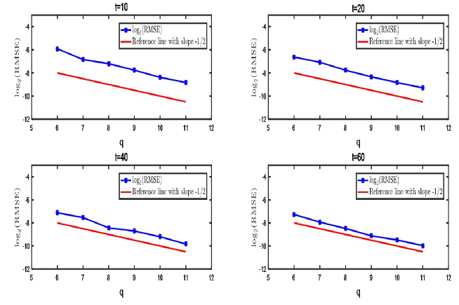
Figure 1: The functions $\log_{2}(RMSE)$ of $q=5,6,7,8,9,10,11$ at $t=10,20,40$ and $60$.

Example 6.2.

Consider the following MV-SDE

$$\mathrm{d}X_{t}=(-2X_{t}-\mathbb{E}X_{t})\mathrm{d}t+(2-\sqrt{\mathbb{E}|X_{t}|^{2}})\mathrm{d}B(t).$$ (6.2)

It is straight to verify that MV-SDE (6.2) satisfies the Assumptions 1 and 2. In addition, from [12], the normal distribution $N(0,4/9)$ is the unique invariant probability measure of MV-SDE (6.2). For any given $\tau>0$, the self-interacting process is

$$\mathrm{d}Y_{t}=\Big{(}-2Y_{t}-\frac{1}{\lfloor t\rfloor_{\tau}+1}\sum_{j=0}^{\lfloor t\rfloor_{\tau}}Y_{j\tau}\Big{)}\mathrm{d}t+\Big{[}2-\Big{(}\frac{1}{\lfloor t\rfloor_{\tau}+1}\sum_{j=0}^{\lfloor t\rfloor_{\tau}}|Y_{j\tau}|^{2}\Big{)}^{\frac{1}{2}}\Big{]}\mathrm{d}B_{t}.$$ (6.3)

By Theorem 3.1, the weighted empirical measure of self-interacting process $Y$

$$\mathcal{E}^{Y}_{\tau,t}(\cdot)=\frac{1}{\lfloor t\rfloor_{\tau}}\sum_{j=1}^{\lfloor t\rfloor_{\tau}}\delta_{Y_{j\tau}}(\cdot)$$

converges to the invariant probability measure $N(0,9/4)$ in $\mathcal{W}_{2}$-Wasserstein distance. Let $\Delta\in(0,1]$ sufficiently small and let $M=\tau/\Delta\in\mathbb{N}_{+}$. Then the EM scheme for self-interacting process $Y$ is defined by

$$\begin{cases}&Z_{0}=X_{0},~{}~{}~{}k=0,1,\cdots,\\ &Z_{k\tau+(m+1)\Delta}=Z_{k\tau+m\Delta}-\Big{(}2Z_{k\tau+m\Delta}+\frac{1}{k+1}\sum_{j=0}^{k}Z_{j\tau}\Big{)}\Delta,\\ &~{}~{}~{}+\Big{[}2-\Big{(}\frac{1}{k+1}\sum_{j=0}^{k}|Z_{j\tau}|^{2}\Big{)}^{\frac{1}{2}}\Big{]}\sqrt{\Delta}\xi^{k}_{m},~{}~{}~{}m=0,1,\cdots,M-1,\end{cases}$$

where $\{\xi^{k}_{m}\}$ is the sequence of i.i.d. Gaussian random variables. Let $\tau=0.5$ and $\Delta=2^{-8}$. We conduct the Jarque-Bera (J-B) test with a significance level of 0.05 by Matlab to confirm that the numerical empirical measure $\mathcal{E}^{Z}_{\tau,t}$ follows a normal distribution for $t=500,1000,2000,4000$.

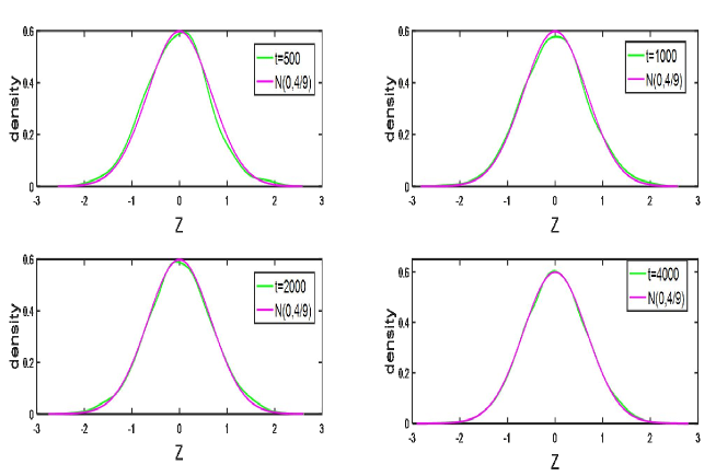
Figure 2: The empirical density functions of self-interacting process at $t=500,1000,2000,4000$ and the normal distribution N(0, 9/4).

To more intuitively illustrate the result of Theorem 4.2, Figure 2 plots numerical empirical density functions of $\mathcal{E}^{Z}_{\tau,t}$ at time $t=500,1000,2000$ and $4000$ the density function of normal distribution $N(0,4/9)$, respectively. As can be seen from Figure 2, as the time $t$ increases, the shape of the empirical density function becomes increasingly close to the density function of normal distribution $N(0,4/9)$.

In addition, let $\tau=0.5$, $t=100$ and $\Delta=2^{-8}$. We further compare the averaged weighted empirical measures of the multi-particle systems for $N=1,50,100$ and $N=200$. We use the J-B test to examine that the averaged weighted empirical measures of the multi-particle systems, all of which are normal distributions for $N=1,50,100,200$. Furthermore, Figure 3 plots their empirical density functions and the normal distribution $N(0,4/9)$, respectively. One observes that as the particle number $N$ increases, the shape of the empirical density function becomes increasingly close to the density function of normal distribution $N(0,4/9)$.

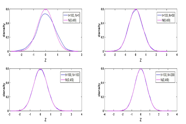
Figure 3: The empirical density functions of multi-particle system at $t=100$ for $N=1,50,100,200$ and the normal distribution $N(0,4/9)$.

References

- [1] N. U. Ahmed, X. Ding, On invariant measures of nonlinear Markov processes, J. Appl. Math. Stoch. Anal. 6 (1993): 385–406.
- [2] F. Antonelli, A. Kohatsu-Higa, Rate of convergence of a particle method to the solution of the McKean-Vlasov equation, Ann. Appl. Probab., 2002 (12): 423-476.
- [3] J. Bao, M. Scheutzow, C. Yuan, Existence of invariant probability measures for functional McKean-Vlasov SDEs, Electron. J. Probab., 27 (2022): 1083-6489.
- [4] J. Bao, X. Huang, Approximations of McKean-Vlasov stochastic differential equations with irregular coefficients, J. Theoret. Probab., 2022 (35): 1187-1215.
- [5] G. Ben Arous, O. Zeitouni, Increasing propagation of chaos for mean field models, Ann. Inst. H. Poincaré Probab. Statist., 35 (1999): 85-102.
- [6] R. J. Berman, M. Önnheim, Propagation of chaos for a class of first order models with singular mean field interactions, SIAM J. Math. Anal., 51 (2019): 159-196.
- [7] M. Bossy, D. Talay, A stochastic particle method for the Mckean-Vlasov and the Burgers equation, Math. Comp., 66 (1997), 157–192.
- [8] L.-P. Chaintron, A. Diez, Propagation of chaos: a review of models, methods and applications. I. Models and methods, arXiv preprint arXiv: 2203.00446, (2022).
- [9] M. Chen, From Markov Chains to Non-equilibrium Particle Systems, Second edition. Singapore: World Scientific, 2004.
- [10] X. Ding, H. Qiao, Euler-Maruyama approximations for stochastic McKean-Vlasov equations with non-Lipschitz coefficients, J. Theoret. Probab., 34 (2021): 1408-1425.
- [11] G. Dos Reis, S. Engelhardt, G. Smith, Simulation of McKean–Vlasov SDEs with super-linear growth, IMA J. Numer. Anal., 42 (2022): 874–922.
- [12] K. Du, Y. Jiang, J. Li, Empirical approximation to invariant measures for McKean-Vlasov processes: mean-field interaction vs self-interaction, Bernoulli, 29 (2023): 2492-2518.
- [13] K. Du, Y. Jiang, X. Li, Sequential propagation of chaos, arXiv preprint arXiv: 2301.09913v1, 2023.
- [14] W. R. P. Hammersley, D. Šiška, L. Szpruch, McKean-Vlasov SDEs under measure dependent Lyapunov conditions, Ann. Inst. Henri Poincaré Probab. Stat., 57 (2021): 1032-1057.
- [15] A. Kolmogoroff, Über die analytischen Methoden in der Wahrscheinlichkeitsrechnung, Math. Ann., 104 (1931): 415-458.
- [16] C. Kumar, Neelima, C. Reisinger, W. Stockinger, Well-posedness and tamed schemes for McKean-Vlasov equations with common noise, Ann. Appl. Probab., 32 (2022): 3283-3330.
- [17] C. Kumar, Neelima, On explicit Milstein-type scheme for McKean-Vlasov stochastic differential equations with super-linear drift coefficient, Electron. J. Probab., 26 (2021): 1083-6489.
- [18] D. Lacker, On a strong form of propagation of chaos for McKean-Vlasov equations, Electron. Commun. Probab., 23 (2018): Paper No. 45.
- [19] D. Lacker, L. Le Flem, Sharp uniform-in-time propagation of chaos, Probab. Theory Related Fields, 187 (2023): 443-480.
- [20] M. Liang, M. B. Majka, J. Wang, Exponential ergodicity for SDEs and McKean–Vlasov processes with Lévy noise, Ann. Inst. Henri Poincaré Probab. Stat., 57 (2021): 1665-1701.
- [21] W. Liu, L. Wu, C. Zhang, Long-time behaviors of mean-field interacting particle systems related to McKean-Vlasov equations, Comm. Math. Phys., 387 (2021): 179-214.
- [22] H.P. McKean, Propagation of chaos for a class of non-linear parabolic equations, in: Stochastic Differential Equations (Lecture Series in Differential Equations, Session 7, Catholic Univ., 1967), 1967, pp. 41–57.
- [23] H. P. McKean, A class of Markov processes associated with nonlinear parabolic equations, Proc. Nat. Acad. Sci. U.S.A., 56 (1966): 1907-1911.
- [24] A.-S. Sznitman, Topics in propagation of chaos, in: Paul-Louis Hennequin (Ed.), Ecole d’Eté de Probabilités de Saint-Flour XIX — 1989, Springer Berlin Heidelberg, Berlin, Heidelberg, 1991, pp. 165–251.
- [25] Veretennikov, A.Y. (2006). On ergodic measures for McKean-Vlasov stochastic equations. In Monte Carlo and Quasi-Monte Carlo Methods, Berlin: Springer, 2004, pp. 471–486.
- [26] Wang F., Distribution dependent SDEs for Landau type equations, Stochastic Process and their Applications, 128 (2018): 595-621.
- [27] F. Wang, Exponential ergodicity for non-dissipative McKean-Vlasov SDEs, Bernoulli, 29 (2023):1035–1062.
- [28] Hutzenthaler M, Jentzen A, Kloeden P E. Strong and weak divergence in finite time of Euler’s method for stochastic differential equations with non-globally Lipschitz continuous coefficients [J]. Proceedings A, 2011, 467: 1563–1576.
- [29] Bao J., Reisinger C., Ren P., Stockinger W. First order convergence of Milstein schemes for McKean–Vlasov equations and interacting particle systems, Proceedings A, 471 (2021): 20200258.
- [30] Chen X., Dos Reis G., A flexible split-step scheme for solving McKean-Vlasov stochastic differential equations, Appl. Math. Comput., 427 (2022): 127180, 23 pp.
- [31] Veretennikov, A. Y., On ergodic measures for McKean-Vlasov stochastic equations. In Monte Carlo and Quasi-Monte Carlo Methods, 2004: 471-486, Springer-Verlag, Berlin, 2006.