Variational Improvement of the Hartree-Fock Approach to the 2D Hubbard Model

Abstract

We consider a refinement of the usual Hartree-Fock method applied the 2D Hubbard model, in Nambu spinor formulation. The new element is the addition of a “condensate inducing” term proportional to a variational parameter $h$ to the Hartree-Fock Hamiltonian, which generates an s- or d-wave condensate. This modified Hartree-Fock Hamiltonian is used only to generate variational trial states; energy expectation values are computed in the full two-dimensional Hubbard Hamiltonian with no modification. It is found that there exist trial states with non-vanishing condensates that are significantly lower in energy than the standard Hartree-Fock ground states, in some range of the $U/t$-density plane.

There is still some question about whether, and for which parameter values, the ground state of the two-dimensional Hubbard model exhibits the d-wave condensation observed in cuprate superconductors. The model is difficult to solve convincingly due to the sign problem, and all existing methods seem to have their limitations, both theoretical and practical. The earliest approach, dating to 1966, is the Hartree-Fock method applied to the Hubbard model, and this venerable approach has a very large literature, a sample of which is Penn ; *Hirsch; *Poilblanc; *Zaanen; *Machida; *Schulz1; *Schulz2; *Ichimura; *Verges; *Inui; *Dasgupta; *Xu. Two contributions of ours along these lines are in Matsuyama:2022kam ; Matsuyama:2022dtd . The strengths and limitations of the Hartree-Fock method are well known, and are described in a number of reviews Scalettar ; Powell ; Lechermann ; Imada ; Fazekas . Like any mean field approach the method neglects correlations, and in addition uses a single Slater determinant to approximate what is surely a more complex ground state. Nevertheless, this method was successful in predicting stripe patterns (Zaanen and Gunnarsson, Poilblanc and Rice in Zaanen ) later observed in experiment Emery , as well as the emergence of ferromagnetism and the relation to the Stoner criterion. So it is of interest to see how far one can go with a single Slater determinant, in particular whether the existing Hartree-Fock approach can be significantly improved, and whether an improved approach can tell us anything about d-wave condensation and superconductivity.

We begin with the 2D Hubbard model, in Nambu spinor formalism Matsuyama:2022dtd

$$H = -t\sum_{<xy>}\{\psi^{\dagger}_{1}(x)\psi_{1}(y)-\psi^{\dagger}_{2}(x)\psi_{2}(y)\}$$ (1)

$$+U\sum_{x}\psi^{\dagger}_{1}(x)\psi_{1}(x)-U\sum_{x}\psi^{\dagger}_{1}(x)\psi_{1}(x)\psi^{\dagger}_{2}(x)\psi_{2}(x)$$

$$-\mu\sum_{x}\{\psi^{\dagger}_{1}(x)\psi_{1}(x)+1-\psi^{\dagger}_{2}(x)\psi_{2}(x)\}\ ,$$

where $\psi_{1},\psi_{2}$ are the upper and lower components, respectively, of the Nambu spinor $\psi$, $\mu$ is the chemical potential, and we neglect any hopping terms beyond nearest neighbor. We recall the definitions

$$\psi(x) = \left[\begin{array}[]{c}c_{\uparrow}(x)\cr c^{\dagger}_{\downarrow}(x)\end{array}\right]~{}~{}~{},~{}~{}~{}\psi^{\dagger}(x)=[c^{\dagger}_{\uparrow}(x),c_{\downarrow}(x)]\ ,$$ (4)

where $c^{\dagger}_{s}(x),c_{s}(x)$ are the usual electron creation/destruction operators. The trial (“Slater determinant”) state is

$$|\Omega\rangle=\prod_{i=1}^{M}\bigg{(}\sum_{x_{i},\alpha_{i}}\phi_{i}(x_{i},\alpha_{i})\psi^{\dagger}_{\alpha_{i}}(x_{i})\bigg{)}|0\rangle\ .$$ (6)

Note that the Fock vacuum $|0\rangle$ in Nambu formulation, annihilated by all $\psi$ operators, differs from the no-electron Fock vacuum in standard formulation. $|\Omega\rangle$ is not an eigenstate of particle number, in the Nambu formulation, but it is an eigenstate of the difference of electron spin up/down number operators $N_{\uparrow}-N_{\downarrow}$. Setting $M=L^{2}$ restricts to states with an absence of overall magnetic moment (equal numbers of spin up and down), with the expectation value of electron density controlled by the chemical potential $\mu$. In the Hartree-Fock approach the one-particle wave functions $\phi_{i}(x_{i},\alpha_{i})$ are to be determined self-consistently, and defining

$$\rho(x,\alpha\beta) = \langle\Omega|\psi^{\dagger}_{\alpha}(x)\psi_{\beta}(x)|\Omega\rangle\ ,$$ (7)

the Hartree-Fock Hamiltonian is

$$H_{HF}(\Omega)$$ (8)

$$= -t\sum_{<xy>}(\psi_{1}^{\dagger}(x)\psi_{1}(y)-\psi_{2}^{\dagger}(x)\psi_{2}(y))$$

$$-\mu\sum_{x}(\psi_{1}^{\dagger}(x)\psi_{1}(x)-\psi_{2}^{\dagger}(x)\psi_{2}(x))$$

$$+U\sum_{x}\bigg{\{}[1-\rho(x,22)]\psi^{\dagger}_{1}(x)\psi_{1}(x)-\rho(x,11)\psi^{\dagger}_{2}(x)\psi_{2}(x)$$

$$\qquad\qquad+\rho(x,12)\psi^{\dagger}_{2}\psi_{1}+\rho(x,21)\psi_{1}^{\dagger}\psi_{2}\bigg{\}}$$

$$= \sum_{x}\sum_{y}\psi^{\dagger}_{\alpha}(x)[H]_{x\alpha,y\beta}\psi_{\beta}(y)\ .$$

There is no obvious evidence of a condensate in the ground state of the Hartree-Fock Hamiltonian, in either conventional Penn ; *Poilblanc; *Zaanen; *Machida; *Schulz1; *Schulz2; *Ichimura; *Verges; *Inui; *Dasgupta; *Xu or Nambu spinor Matsuyama:2022dtd formulation. In general, in Nambu formulation, a condensate exists if there are one-particle states in the Slater determinant such that $\phi_{i}(x,\alpha)\neq 0$ for both indices $\alpha=1,2$ (see eq. (13) below). But it is clear from inspection of (6), (7), (8) that Hartree-Fock self-consistency allows that each $\phi_{i}(x,\alpha)$ is nonzero for only one of the two indices $\alpha=1,2$ (and $\rho(x,12)=\rho^{*}(x,21)=0$). In that case there is no condensate in this mean field approach.

With this in mind, let us modify $H_{HF}$ by adding a “condensate inducing” term to the matrix $[H]_{x\alpha,x^{\prime}\beta}$

$$[V]^{cond}_{x\alpha,x^{\prime}\beta} = h(\delta_{\alpha 1}\delta_{\beta 2}+\delta_{\alpha 2}\delta_{\beta 1})$$ (9)

$$\times (\delta_{x,x^{\prime}+\hat{e}_{x}}+\delta_{x,x^{\prime}-\hat{e}_{x}}+q\delta_{x,x^{\prime}+\hat{e}_{y}}+q\delta_{x,x^{\prime}-\hat{e}_{y}})\ ,$$

where $\hat{e}_{x},\hat{e}_{y}$ are unit vectors in the $x,y$ directions respectively, $q=\pm 1$, and $h$ is a variational parameter. We will denote the modified Hartree-Fock Hamiltonian as $H_{HFq}$. If we make the special assumption that the $\rho(x,\alpha\beta)=\rho(\alpha\beta)$ are position independent (an assumption which is simply not true in the stripe and antiferromagnetic phases) then it is not hard to see that the ground state of $H_{HF-}$ will have a d-wave condensate in the neighborhood of the Fermi surface, even in the limit $h\rightarrow 0$. This result, which follows from degenerate perturbation theory, can be seen as follows: Translation invariance of $\rho$ implies that $[H]$ is diagonalized by momentum eigenstates, and on an $L\times L$ lattice, in the basis

$$\phi_{1}(k)={1\over L}\left[\begin{array}[]{c}e^{i\bm{k}\cdot\bm{x}}\cr 0\end{array}\right]~{}~{}~{},~{}~{}~{}\phi_{2}(k)={1\over L}\left[\begin{array}[]{c}0\cr e^{i\bm{k}\cdot\bm{x}}\end{array}\right]\ ,$$ (10)

the matrix $[H]$ is decomposed, at each $k$, into blocks

$$[H]_{k}=\left[\begin{array}[]{cc}\epsilon^{1}_{k}&2h(\cos(k_{x})-\cos(k_{y}))\cr 2h(\cos(k_{x})-\cos(k_{y}))&\epsilon^{2}_{k}\end{array}\right]\ ,$$ (11)

where

$$\epsilon^{1}_{k} = -2t((\cos(k_{x})+\cos(k_{y}))+Un_{\downarrow}-\mu$$

$$\epsilon^{2}_{k} = \ \ \ 2t((\cos(k_{x})+\cos(k_{y}))-Un_{\uparrow}+\mu\ ,$$ (12)

and where $n_{\uparrow}=\rho(11);n_{\downarrow}=1-\rho(22)$ are the expectation values of the number densities of up and down electrons, respectively. In the absence of net magnetization, these numbers are equal. In that case $\epsilon^{2}_{k}=-\epsilon^{1}_{k}$.

The pairing condensate in momentum space is

$$P(\mathbf{p}) = {1\over L^{2}}\sum_{x}\sum_{x^{\prime}}\langle\Omega|c^{\dagger}_{\uparrow}(x)c^{\dagger}_{\downarrow}(x^{\prime})|\Omega\rangle e^{i\mathbf{p}\cdot(\mathbf{x}-\mathbf{x}^{\prime})}$$ (13)

$$= {1\over L^{2}}\sum_{x}\sum_{x^{\prime}}\langle\Omega|\psi^{\dagger}_{1}(x)\psi_{2}(x^{\prime})|\Omega\rangle e^{i\mathbf{p}\cdot(\mathbf{x}-\mathbf{x}^{\prime})}$$

$$= {1\over L^{2}}\sum_{x}\sum_{x^{\prime}}\sum_{i=1}^{L^{2}}\phi_{i}^{*}(x,1)\phi_{i}(x^{\prime},2)e^{i\mathbf{p}\cdot(\mathbf{x}-\mathbf{x}^{\prime})}$$

$$= {1\over L^{2}}\sum_{i=1}^{L^{2}}\phi_{i}^{*}(p,1)\phi_{i}(p,2)\ .$$

As $h\rightarrow 0$ the wavefunctions (10) are eigenstates of $[H]_{k}$, in which case $P(\mathbf{p})=0$, and there is no condensate except at momenta where $\epsilon^{1}_{k}=\epsilon^{2}_{k}$. For $\langle N_{\uparrow}-N_{\downarrow}\rangle=0$, and denoting the electron number density on an $L\times L$ periodic lattice as

$$f = \langle N_{\uparrow}+N_{\downarrow}\rangle/L^{2}$$ (14)

$$= \sum_{x}\langle\Omega|\psi^{\dagger}_{1}(x)\psi_{1}(x)-\psi^{\dagger}_{2}(x)\psi_{2}(x)+1|\Omega\rangle$$

$$= {1\over L^{2}}\sum_{x}\{\rho(x,11)-\rho(x,22)+1\}\ ,$$

the condition is

$$2t((\cos(k_{x})+\cos(k_{y}))-\frac{1}{2}Uf+\mu=0\ ,$$ (15)

which we refer to as the Fermi surface. Precisely on the Fermi surface, degenerate perturbation theory gives us new eigenstates $\phi^{\prime}_{\pm}(k)=(1/\sqrt{2})(\phi_{1}(k)\pm\phi_{2}(k))$, resulting in a non-zero condensate. This is sufficient to change the condensate pattern dramatically for any finite $h$, no matter how small, and as $h\rightarrow 0$ we find Matsuyama:2022dtd

$$P(\mathbf{k})=\left\{\begin{array}[]{cl}\frac{1}{2}\text{sign}(\cos k_{x}-\cos k_{y})&\mathbf{k}\in\text{Fermi surface}\cr 0&\text{otherwise}\end{array}\right.\ ,$$ (18)

a result which is strongly reminiscent of d-wave pairing. Since this seems to be a case where the slightest perturbation breaks a ground state degeneracy, even as the strength of the breaking terms goes to zero, it is tempting to regard this situation as an example of spontaneous symmetry breaking. In fact this argument was already presented in Matsuyama:2022dtd , but there are two objections. First, the densities $\rho(x,\alpha\beta)$ are not necessarily translation invariant, e.g. in the stripe phase, yet there can be superconductivity in that phase. But the more serious objection is that if we take the $h\rightarrow 0$ limit, then by this argument the condensate only exists exactly at the Fermi surface. In that case the condensate density vanishes in the infinite volume limit.

These objections suggest a change in philosophy: why should we take the $h\rightarrow 0$ limit? The real objective is to find the best possible approximation, within the limitations dictated by a single Slater determinant, to the ground state of the full $h$-independent Hubbard Hamiltonian of (1). Then the question is whether mixing one-particle states in the neighborhood of the Fermi surface, which is what the condensate-inducing term achieves, would lower the expectation value of the Hubbard Hamiltonian. If so, then since the mixed states would have non-zero amplitudes for both $\alpha$ index values, a condensate is obtained. So let us regard the ground state of $H_{HFq}$, denoted $|\Omega_{h}\rangle$, as a trial wave functional, dependent on the variational parameter $h$. If energy expectation value $\mathcal{E}(h)=\langle\Omega_{h}|H|\Omega_{h}\rangle$ of the full Hubbard Hamiltonian is minimized at some $h>0$, then by the rules of the variational approach the ground state $|\Omega_{h}\rangle$ is a better approximation, as compared to the Hartree-Fock ground state $|\Omega_{0}\rangle$, to the true ground state of the Hubbard Hamiltonian. Then the procedure is to choose some set of parameters $\{U,\mu\}$ (setting $t=1$ for numerical work), and at each $U,\mu$ and variational parameter $h$ we compare $\mathcal{E}(0)$ to (i) $\mathcal{E}(h)$ for the ground state $|\Omega_{h}\rangle$ of $H_{HF-}$, associated with a d-wave condensate; and (ii) $\mathcal{E}(h)$ for the ground state $|\Omega_{h}\rangle$ of $H_{HF+}$, associated with an s-wave condensate. If $h>0$ is energetically favorable, in cases (i) and/or (ii), we choose the value of $h$ and sign of $q$ which gives the lowest $\mathcal{E}$. Whichever ground state has the lowest $\mathcal{E}$ is the state which is favored at the given $U,\mu$, at the electron density $f$ in (14). We again emphasize that the $h$ parameter is absent in the Hubbard Hamiltonian $H$, and only appears as a label of the choice of trial ground state.

The calculations were carried out on $16\times 16$ lattices with periodic boundary conditions, and our results are shown in the $U-\mu$ plane in Fig. 1, and in the $U-f$ (coupling-density) plane in Fig. 2, where $f=1$ is half-filling. Each of the symbols in Fig. 1 represents a pair of $U,\mu$ values where we have carried out the calculation described above. At the filled square locations, $\mathcal{E}(h)$ for ${q=-1}$, i.e. d-wave, is lower in energy than either $q=1$ (s-wave) or $h=0$ (standard Hartree-Fock). At filled circle locations, $\mathcal{E}(h)$ is lowest for an s-wave condensate. The open square symbols represent locations where standard Hartree-Fock, i.e. $h=0$ with no condensate, have the lowest energy. On average the fractional decrease in energy of the condensate states, as compared to the conventional ($h=0$) states at the same $U,\mu$ values, is 1.3%. The optimum $h$ varies, but is generally $O(10^{-2})$. Qualitatively, from Fig. 2, we see that the condensate disappears completely at low $U<2$ and high $U>10$ values of $U$, and at densities below half-filling. Obviously, with a finite set of $\mu$ values we have not covered the entire $U-\mu$ plane, although nearby filled symbols at a given $U$ probably indicate a continuum of densities with condensate states.

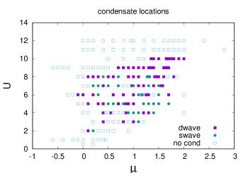
Figure 1: Numerical calculations were carried out the points indicated in the $U-\mu$ plane. Filled squares indicate d-wave condensates, filled circles indicate s-wave condensates, open symbols indicate that the no-condensate state at $h=0$ has the lowest energy expectation value $\mathcal{E}$.

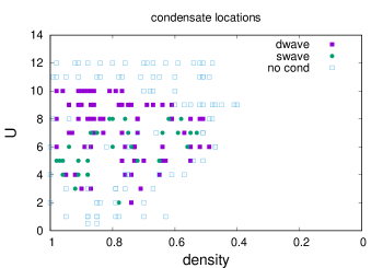
Figure 2: Data obtained at the $U,\mu$ values shown in Fig. 1 are each associated with a density $f$. In this figure the same points are plotted in the $U-f$ plane.

The momentum-space distribution of the condensate is quite different at low and high $U$. An example at $U=2$ and density $0.74$ is shown in Fig. 3. Here the condensate seems to be concentrated mainly at the Fermi surface, moreover the pattern of up/down spins has a stripe pattern, as seen in Fig. 4, which displays the average spin/local magnetization

$$D(x) = \langle c^{\dagger}_{\uparrow}(x)c_{\uparrow}(x)\rangle-\langle c^{\dagger}_{\downarrow}(x)c_{\downarrow}(x)\rangle$$ (19)

$$= \langle\psi_{1}^{\dagger}(x)\psi_{1}(x)\rangle+\langle\psi_{2}^{\dagger}(x)\psi_{2}(x)\rangle-1$$

$$= \rho(x,11)+\rho(x,22)-1\ .$$

In contrast, the condensate distribution at $U=9$ and density $0.67$ which is displayed in Fig. 5, is much more diffuse, and the pattern of spins (Fig. 6) is a little harder to characterize. But it is clear that in both cases the expectation value of spin densities is not at all space independent. We see that the amplitude of the condensate at small $U=2$, which is concentrated at the Fermi surface, is much larger than the amplitude of the condensate in the more diffuse result at $U=9$. But if one defines a measure of total condensate

$$C={1\over L^{2}}\sum_{k}|P(k)|\ ,$$ (20)

then the measures at $U=2$ and $U=9$ are comparable, with $C=0.015$ and $C=0.010$ respectively.

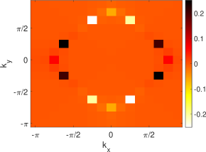
Figure 3: Momentum space condensate $P(k)$ at $U=2,\mu=0.1$, where we find density $f=0.74$.

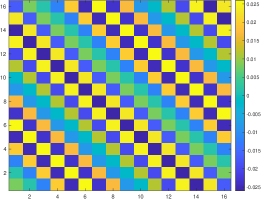
Figure 4: Spin average $D(x)$ on the $16\times 16$ lattice at parameters ${U=2,\mu=0.1}$.

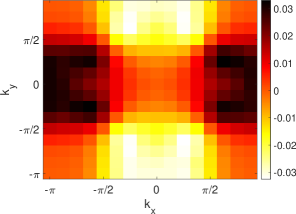
Figure 5: Momentum space condensate $P(k)$ at $U=9,\mu=0.9$, where we find density $f=0.67$.

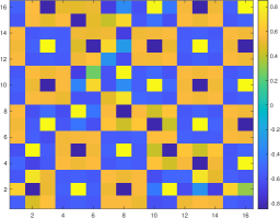
Figure 6: Spin average $D(x)$ on the $16\times 16$ lattice at parameters ${U=9,\mu=0.9}$.

Since a slight variational improvement of the Hartree-Fock approach yields both s- and d-wave condensates, a natural question is whether we can find a more systematic procedure for obtaining the optimal approximation to the ground state, rather than depending on the choice of a specific condensate-inducing term which, of course, may not be the ideal choice. To improve matters, the general idea is still to combine the Hartree-Fock and variational approaches to optimize a single determinant approximation to the ground state. A maximal (and impractical) procedure would be as follows: On a finite $L\times L$ lattice at fixed $U$ and $\mu$, we apply the Hartree-Fock method to obtain a complete and orthogonal set of of one-particle wave functions $\{\phi_{n}(x,\alpha),n=1,2,...,2L^{2}\}$. The standard Hartree-Fock ground state is shown in (6). Any other Slater determinant can be obtained by replacing the set $\{\phi_{n}\}$ in (6) by a new set $\{\phi^{\prime}_{n}=U_{nm}\phi_{m}\}$, where $U=\exp(i\gamma_{i}T_{i})$ is a $2L^{2}\times 2L^{2}$ unitary matrix which is a member of the $U(N)$ group, with $\{T_{i}\}$ the corresponding generators. Then we may regard the $\gamma_{i}$ as variational parameters, and attempt to vary those parameters in such a way as to minimize the expectation value $\mathcal{E}=\langle\Omega|H|\Omega\rangle$, building $|\Omega\rangle$, as before, out of a subset of the $\{\phi^{\prime}_{n}\}$. In principle, if one could find the set of $\gamma$’s which minimizes $\mathcal{E}$, that would be the best approximation, by a single Slater determinant, to the true ground state of the Hubbard Hamiltonian. In practice there will be a vast number of local minima, but aside from that this “brute force” approach, with the number of variational parameters equal to $4L^{4}$, seems extremely computation intensive. But if it would be the case that the Hartree-Fock approach is only failing close to the Fermi surface, then the problem may be more tractable. For most one-particle states we let $\phi^{\prime}_{n}=\phi_{n}$, and only choose a subset of $K$ one-particle states, in the immediate neighborhood of the Fermi surface, for which we consider $\phi^{\prime}=U\phi$. This time, $U$ is only a $K\times K$ matrix acting on states in the Hilbert space spanned by the $K$ Hartree-Fock one-particle states near the Fermi surface. Of course this still leaves $K^{2}$ variational parameters, but one can imagine some stochastic or relaxation approach which would converge to at least a local minimum. For example, one could cycle through pairs of one particle states in the $K$ subset, and apply at each stage an SU(2) transformation to obtain a new pair of states which are linear combinations of the original pair. These could be accepted, as new one particle states in the Slater determinant, if they lower $\mathcal{E}$. One would of course have to test the sensitivity of the final result to the choice of $K$, to ensure that enough states were chosen.

We leave this last suggestion for future investigation.

- (1) D. R. Penn, Phys. Rev. 142, 350 (1966).
- (2) J. E. Hirsch, Phys. Rev. B 31, 4403 (1985).
- (3) D. Poilblanc and T. M. Rice, Phys. Rev. B 39, 9749 (1989).
- (4) J. Zaanen and O. Gunnarsson, Phys. Rev. B 40, 7391 (1989).
- (5) K. Machida, Physica C: Superconductivity 158, 192 (1989).
- (6) H. Schulz, Journal de Physique 50, 2833 (1989).
- (7) H. J. Schulz, Phys. Rev. Lett. 64, 1445 (1990).
- (8) M. Ichimura, M. Fujita, and K. Nakao, Journal of the Physical Society of Japan 61, 2027 (1992), https://doi.org/10.1143/JPSJ.61.2027.
- (9) J. Vergés, E. Louis, P. Lomdahl, F. Guinea, and A. Bishop, Physical Review B 43, 6099 (1991).
- (10) M. Inui and P. Littlewood, Physical Review B 44, 4415 (1991).
- (11) C. Dasgupta and J. Halley, Physical Review B 47, 1126 (1993).
- (12) J. Xu, C.-C. Chang, E. J. Walter, and S. Zhang, Journal of Physics: Condensed Matter 23, 505601 (2011).
- (13) K. Matsuyama and J. Greensite, Annals Phys. 442, 168922 (2022), arXiv:2201.05750.
- (14) K. Matsuyama and J. Greensite, Annals Phys. 458, 169456 (2023), arXiv:2210.06674.
- (15) R. Scalettar, An introduction to the hubbard model, in Quantum Materials: Experiments and Theory, edited by E. Pavarini, E. Koch, J. van den Brink, and G. Sawatzky, 2016.
- (16) B. J. Powell, An introduction to effective low-energy hamiltonians in condensed matter physics and chemistry, 2010, arXiv:0906.1640.
- (17) F. Lechermann, Model hamiltonians and basic techniques, in The LDA+DMFT approach to strongly correlated materials, edited by E. Pavarini, E. Koch, and A. Lichtenstein, 2011.
- (18) M. Imada, A. Fujimori, and Y. Tokura, Rev. Mod. Phys. 70, 1039 (1998).
- (19) P. Fazekas, Lecture Notes on Electron Correlation and Magnetism (WORLD SCIENTIFIC, 1999), https://www.worldscientific.com/doi/pdf/10.1142/2945.
- (20) V. Emery, S. Kivelson, and J. Tranquada, Proc. Natl. Acad. Sci. USA 96(16), 8814 (1999).