Bipartite causal inference with interference, time series data, and a random network

Abstract

In bipartite causal inference with interference there are two distinct sets of units: those that receive the treatment, termed interventional units, and those on which the outcome is measured, termed outcome units. Which interventional units’ treatment can drive which outcome units’ outcomes is often depicted in a bipartite network. We study bipartite causal inference with interference from observational data across time and with a changing bipartite network. Under an exposure mapping framework, we define causal effects specific to each outcome unit, representing average contrasts of potential outcomes across time. We establish unconfoundedness of the exposure received by the outcome units based on unconfoundedness assumptions on the interventional units’ treatment assignment and the random graph, hence respecting the bipartite structure of the problem. By harvesting the time component of our setting, causal effects are estimable while controlling only for temporal trends and time-varying confounders. Our results hold for binary, continuous, and multivariate exposure mappings. In the case of a binary exposure, we propose three matching algorithms to estimate the causal effect based on matching exposed to unexposed time periods for the same outcome unit, and we show that the bias of the resulting estimators is bounded. We illustrate our approach with an extensive simulation study and an application on the effect of wildfire smoke on transportation by bicycle.

1 Introduction

Causal inference methodology most often focuses on the scenario where units are assigned to treatment or control, and an outcome is measured on the same set of units. However, in some cases, the units that receive the treatment are distinct from the units that experience the outcome. We refer to the former as interventional units, and the latter as outcome units. The outcome units, which do not get treatment themselves, are exposed to the treatment only through their connections to potentially treated interventional units. The causal dependencies across units can be described in a bipartite network, and, as a result, this setting has been termed bipartite interference (Zigler and Papadogeorgou, 2021).

In this manuscript, we focus on bipartite causal inference with interference from observational data measured over time and a varying bipartite network. Each interventional unit receives a treatment level which can change over time according to an unknown assignment mechanism that depends on covariates of the interventional units, the outcome units, and the network. At each time, the bipartite network of causal dependencies across units is specified by a random process which itself can depend on all the covariates. By considering an evolving network and temporal variations in the treatment assignment, we provide a comprehensive framework for analyzing bipartite interference with temporal data.

Existing work in causal inference with bipartite interference is cross-sectional and considers a fixed and known bipartite network. Zigler and Papadogeorgou (2021) introduced causal estimands for bipartite causal inference, and developed weighting-based estimators for the case of clustered interference. Other work in bipartite causal inference adopted the notion of an exposure mapping (e.g., Aronow and Samii, 2017; Forastiere et al., 2021) to the bipartite setting, and specified that potential outcomes depend on interventional units’ treatment levels through known functions of the treatment and the bipartite network. In Zigler et al. (2020), the exposure bipartite network describes complex atmospheric and geographic dependencies among units. In the experimental setting, under a linear exposure mapping, Harshaw et al. (2023) designed estimators and inferential techniques for the effect of assigning all or none of the interventional units to treatment. Pouget-Abadie et al. (2019) and Harshaw et al. (2023) developed experimentation techniques that improve efficiency of estimators, while Brennan et al. (2022) focused on avoiding inferential bias due to interference. Doudchenko et al. (2020) proposed using propensity scores to account for confounding of a unit’s exposure due to the network structure. All these studies are cross-sectional and the network of causal dependencies is fixed.

For time series data, most of the causal inference literature focuses on the case without interference. The literature on this topic is large, and it is out of scope to review here (see Abadie and Cattaneo, 2018; Imbens, 2024, for surveys on the topic). Relevant to our work are extensions of panel data methodology to the case with unit-to-unit interference where a subset of units receives the treatment at some point in time and remain treated thereafter (Cao and Dowd, 2019; Grossi et al., 2020; Di Stefano and Mellace, 2020; Menchetti and Bojinov, 2020), or the units’ treatment assignments changes over time by either endogenous nature or by design (Clark and Handcock, 2021; Agarwal et al., 2023). None of these methods has been considered in the bipartite setting or under a random network.

This work develops a causal inference framework for bipartite interference with time series observational data and a random bipartite network, which allows researchers to capture the dynamic nature of causal relationships in real-world settings where networks and treatment assignments change over time. Our contributions are the following: (a) Under an exposure mapping framework, we define causal estimands of interest for each outcome unit in the bipartite temporal setting as contrasts of the unit’s potential outcomes under different exposure levels, averaged over time (Section 2). (b) We introduce the causal assumptions of unconfoundedness for the treatment and network processes conditional on variables of the interventional units, outcome units and the network. We establish the unconfoundedness for the outcome unit’s exposure, which implies that we can estimate the outcome-unit-specific effects, while conditioning only on temporally-varying information (Section 2). In our work, the unconfoundedness assumptions are at the level on which the randomness occurs (treatment, network), in contrast with existing work that places assumptions on the exposure directly (Zigler et al., 2020; Doudchenko et al., 2020). These results hold for binary, continuous, or multivariate exposures. (c) Focusing on binary exposures, we develop matching procedures to estimate causal effects for each outcome unit (Section 3). The proposed algorithms match an outcome unit’s exposed time periods to unexposed time periods, one-to-one, one-to-two, or one-to-one-or-two, while specifying that matched time periods occur close in time, and satisfy balance constraints for the time-varying covariates. We show that the bias of the matching estimators is bounded, and can be made arbitrarily small by imposing stricter tolerance parameters (Section 3). (d) Our approach infers the causal effect of the interventional units’ treatment on each outcome unit separately. We establish how results on multiple outcome units can be combined to test a global null hypothesis of no treatment effect (Section 3). (e) In an extensive simulation study, we showcase that our approach performs well for estimating the outcome-unit effects, and results in appropriate inference (Section 4). (f) We use our methodology to study whether smoke from wildfires affects the population’s outdoor physical activity in the San Francisco Bay area (Section 5). We find that exposure to smoke from wildfires leads to a decrease in the number of bike rental hours in the city of San Francisco, but does not significantly alter bike use in nearby regions. We conclude with a discussion (Section 6).

2 Bipartite interference with time series and a random network

2.1 The setup

Let $\mathcal{N}=\{n_{1},n_{2},\cdots,n_{N}\}$ denote interventional units followed over time $t=1,2,\cdots,T$. Each of them has a collection of characteristics. We use the superscript ^∗ for time-invariant variables, and the subscript _t for time-specific variables. Let $\bm{X}_{i}^{*}=(X_{i1},X_{i2},\cdots,X_{ip_{X}^{*}})^{\top}$ and $\bm{X}_{ti}=(X_{ti1},X_{ti2},\cdots,X_{tip_{X}})^{\top}$ denote $p_{X}^{*}$ time-invariant and $p_{X}$ time-varying covariates, respectively, for the interventional unit $n_{i}$, and $A_{it}\in\mathcal{A}_{t}$ denote its treatment level at time $t$. For notational simplicity the possible treatment values are assumed constant across time, $\mathcal{A}_{t}=\mathcal{A}$. Let $\bm{X}^{*}=(\bm{X}_{1}^{*\top}\ \bm{X}_{2}^{*\top}\ \cdots\ \bm{X}_{N}^{*\top})^{\top}$ be the $N\times p_{X}^{*}$ matrix of time-invariant covariates, $\bm{X}_{t.}=(\bm{X}_{t1}^{\top}\ \bm{X}_{t2}^{\top}\ \cdots\ \bm{X}_{tN}^{\top})^{\top}$ the $N\times p_{X}$ matrix of time-varying covariates at time $t$, and $\bm{A}_{t}=(A_{t1},A_{t2},\cdots,A_{tN})$ the treatment vector at time $t$, across all interventional units. The interventional units do not experience the outcome.

The set of outcome units is denoted by $\mathcal{M}=\{m_{1},m_{2},\cdots,m_{M}\}$. Each unit $m_{j}$ possesses $p_{W}^{*}$ time-invariant covariates $\bm{W}_{j}^{*}=(W_{j1},W_{j2},\cdots,W_{jp_{W}^{*}})^{\top}$ and $p_{W}$ time-varying covariates $\bm{W}_{tj}=(W_{tj1},W_{tj2},\cdots,W_{tjp_{W}})^{\top}$. We use $\bm{W}^{*}=(\bm{W}_{1}^{*\top}\ \bm{W}_{2}^{*\top}\ \cdots\ \bm{W}_{M}^{*\top})^{\top}$ and $\bm{W}_{t.}=(\bm{W}_{t1}^{\top}\ \bm{W}_{t2}^{\top}\ \cdots\ \bm{W}_{tN}^{\top})^{\top}$ to denote the matrices of dimension $M\times p_{W}^{*}$ and $M\times p_{W}$ of these covariates across the outcome units. For each outcome unit $m_{j}$, we measure an outcome over time, denoted by $Y_{tj}$. We also consider network covariates that describe the relationship between interventional and outcome units. We use $\bm{P}^{*}=\{P^{*}_{ijs}\}$ to denote the $N\times M\times p_{P}^{*}$ array of $p_{P}^{*}$ time-invariant network covariates, and $\bm{P}_{t}=\{P_{tijs}\}$ to denote the $N\times M\times p_{P}$ array of time-varying network covariates at time $t$. Notation like $\bm{P}_{t.j.}=(\bm{P}_{t.j1},\bm{P}_{t.j2},\cdots,\bm{P}_{t.jp_{P}})$ corresponds to the $N\times p_{P}$ sub-matrix of $\bm{P}_{t}$ for outcome unit $m_{j}$.

The random bipartite network can vary over time. Let $\bm{G}_{t}$ denote the $N\times M$ matrix of bipartite connections, where the $(i,j)$ entry is equal to 1, $G_{tij}=1$, if $n_{i}$ and $m_{j}$ are connected at time $t$, and $G_{tij}=0$ otherwise. Then, $\bm{G}_{ti.}=(G_{ti1},\cdots,G_{tiM})^{\top}$ denotes the connectivity vector for interventional unit $n_{i}$ with all the outcome units, and $\bm{G}_{t.j}=(G_{t1j},\cdots,G_{tNj})^{\top}$ denotes the connectivity vector of outcome unit $m_{j}$ with all interventional units, taking values in $\mathcal{G}_{i.}=\{0,1\}^{M}$ and $\mathcal{G}_{.j}=\{0,1\}^{N}$, respectively. The bipartite network need not be binary, and alternative specifications of $\bm{G}$ can be easily incorporated.

The outcome units do not receive an intervention themselves, rather than experience the treatment of the interventional units through the bipartite network. We formalize this using exposure mappings. For the outcome unit $m_{j}$, the function $h_{tj}:\mathcal{A}\times\mathcal{G}_{.j}\rightarrow\mathcal{E}_{tj}$ maps the interventional units’ treatment assignment and the outcome unit’s bipartite connection vector to the outcome unit’s exposure value at time $t$, where $\mathcal{E}_{tj}$ denotes the set of all possible exposure values. Then, $E_{tj}=h_{tj}(\bm{A}_{t},\bm{G}_{t.j})$ is the realized exposure of outcome unit $m_{j}$ at time $t$. The function $h_{tj}(\cdot)$ might return a scalar such as the proportion of interventional units with which $m_{j}$ is connected that are treated. It can also be completely general, specified to return the vector of treatment levels for all connected interventional units, or extended to depend on covariates. We constitute $\bm{E}_{t}=(E_{ti},\cdots,E_{tM})^{\top}$ as the vector (matrix, or collection) of the realized exposure for all $M$ outcome units.

In our study, the interventional units are all forest locations across North America. For these units, time-invariant covariates, $\bm{X}^{*}$, might represent their exact location and species of vegetation. The $M=3$ outcome units represent areas in the San Francisco Bay Area, with potential time-invariant covariates, $\bm{W}^{*}$, that represent demographic and socioeconomic information. Time-varying covariates for both sets of units, $\bm{X}_{t},\bm{W}_{t}$, are weather-related factors, such as temperature and precipitation. Potential network covariates, $\bm{P}^{*}$, include the geographic distance of forest-area pairs. The transformation from wildfire to smoke follows complex chemical and atmospheric reactions, and the resulting smoke can travel long distances, described in the bipartite network $\bm{G}_{t}$. The Hazard Mapping System for smoke (HMS) monitors smoke plumes resulting from fires. HMS implicitly combines the information on the presence of wildfires, $\bm{A}_{t}$, and information on smoke transport, $\bm{G}_{t}$, to deduct the potential smoke exposure in each region in day $t$, $\bm{E}_{t}$. The outcome, $Y_{tj}$, represents daily bike riding hours using Lyft’s Bay Wheels program in each region.

2.2 Potential outcomes and causal estimands

Let $Y_{tj}(\bm{a}_{t},\bm{g}_{t.j})$ denote the potential outcome for unit $m_{j}$ at time $t$ had the treatment of the $N$ interventional units been $\bm{a}_{t}$, and under bipartite connection $\bm{g}_{t.j}$ for unit $m_{j}$. We include the bipartite graph in the notation for potential outcomes to establish that the graph plays a role for how the potential outcomes vary by treatment, but we do not assume that the network is manipulable. The observed outcome corresponds to the potential outcome under the observed treatment and network, as $Y_{tj}=Y_{tj}(\bm{A}_{t},\bm{G}_{t.j})$. This notation implicitly states that previous treatments of the interventional units do not drive the contemporaneous outcome of unit $m_{j}$. We discuss this within the context of our study in Section 5.

Each treatment vector $\bm{a}_{t}$ might lead to a different potential outcome for unit $m_{j}$. The following assumption codifies that the interventional units’ treatment drives potential outcomes only through the resulting outcome unit’s exposure based on the bipartite mapping.

Assumption 1.

For all $\bm{a}_{t},{\bm{a}}_{t}^{\prime}\in\mathcal{A}^{N},$ and $\bm{g}_{t.j},{\bm{g}}_{t.j}^{\prime}\in\mathcal{G}_{.j}$, if $h_{tj}(\bm{a}_{t},\bm{g}_{t.j})=h({\bm{a}}_{t}^{\prime},{\bm{g}}_{t.j}^{\prime})=e_{tj}$, then $Y_{tj}(\bm{a}_{t},\bm{g}_{t.j})=Y_{tj}({\bm{a}}_{t}^{\prime},{\bm{g}}_{t.j}^{\prime})$, and the potential outcome can be denoted as $Y_{tj}(e_{tj})$.

Under 1, the collection of all potential outcomes for outcome unit $m_{j}$ at time $t$ is the set $\mathcal{Y}_{tj}(\cdot)=\{Y_{tj}(e_{tj}),\text{ for }e_{tj}\in\mathcal{E}_{tj}\}$. Similar constructions of exposure mappings and assumptions on the potential outcomes have been discussed in the unipartite (Aronow and Samii, 2017; Forastiere et al., 2021) and bipartite (Zigler et al., 2020; Harshaw et al., 2023; Doudchenko et al., 2020) interference literature. Sävje (2024) discusses the implications of using exposure mappings in the definition of estimands and as assumptions on potential outcomes, providing interesting distinctions between the two.

We consider estimands that are specific to each outcome unit. The contrast $\tau_{tj}(e,e^{\prime})=Y_{tj}(e)-Y_{tj}(e^{\prime})$ represents the fundamental effect of a change in exposure from $e$ to $e^{\prime}$ for the outcome unit $m_{j}$ at time $t$. This unit- and time-specific estimand cannot be estimated without parametric assumptions. Instead, we consider target estimands that represent temporally-average causal effects for unit $m_{j}$ for a change in its exposure value. Specifically,

$$\tau_{j}(e,e^{\prime}) =\frac{1}{T}\sum_{t=1}^{T}\tau_{tj}(e,e^{\prime})=\frac{1}{T}\sum_{t=1}^{T}\left[Y_{tj}(e)-Y_{tj}(e^{\prime})\right],$$

represents the average effect of a change in exposure for unit $$m_{j}$$ across time, and

$$\widetilde{\tau}_{j}(e,e^{\prime}) =\frac{1}{\sum_{t}I(E_{tj}=e)}\sum_{t}\left(Y_{tj}(e)-Y_{tj}(e^{\prime})\right)I(E_{tj}=e)$$

over only those time periods with realized exposure equal to $e$. Therefore, the estimand $\widetilde{\tau}_{j}$ resembles a temporal version of the average treatment effect on the treated. If exposures $e$ and $e^{\prime}$ are not both possible for all time periods, the estimands $\tau_{j}(e,e^{\prime})$ and $\widetilde{\tau}_{j}(e,e^{\prime})$ average over the subset of time periods where both exposure values under investigation are possible.

In Section 3.5, we discuss how focusing on temporally-average estimands might lead to weaker confounding adjustment requirements compared to unit-average estimands.

2.3 Ignorable assignments: assumptions and results

We establish causal unconfoundedness assumptions on the interventional units’ treatment assignment and the random bipartite network that allow us to estimate the estimands of Section 2. We focus on a specific outcome unit $m_{j}$ throughout.

Assumption 2.

(Unconfoundedness of the treatment assignment). The interventional units’ treatment assignment at time $t$ is independent of the potential outcomes of outcome unit $m_{j}$, conditional on a function of time $f(t)$, time-invariant and time-varying covariates of the interventional units, outcome unit $m_{j}$, and their connections, i.e., $P\big{(}\bm{A}_{t}\mid\mathcal{Y}_{tj}(\cdot),f(t),\bm{X}^{*},\bm{X}_{t.},\bm{W}^{*},\bm{W}_{tj},\bm{P}^{*},\bm{P}_{t.j.}\big{)}=P\big{(}\bm{A}_{t}\mid f(t),\bm{X}^{*},\bm{X}_{t.},\bm{W}^{*},\bm{W}_{tj},\bm{P}^{*},\bm{P}_{t.j.}\big{)}$.

Under 2, the treatment assignment mechanism allows for the treatment level of interventional units to be driven by their individual characteristics, characteristics of the outcome units, and general temporal trends such as those that alter the overall prevalence of treatment. Therefore, the permitted treatment assignment mechanisms allow for complex bipartite dependencies that relate units from the two ends of the graph.

Assumption 3.

(Unconfoundedness of the bipartite network). The bipartite connection vector for unit $m_{j}$ is independent of the unit’s potential outcomes given the treatment assignment, temporal trends $f(t)$, and characteristics of all interventional units, the outcome unit $m_{j}$, and their connections, i.e., $\displaystyle P\big{(}\bm{G}_{t.j}|\mathcal{Y}_{tj}(\cdot),\bm{A}_{t},f(t),\bm{X}^{*},\bm{X}_{t.},\bm{W}^{*},\bm{W}_{tj},\bm{P}^{*},\bm{P}_{t.j.}\big{)}=P\big{(}\bm{G}_{t.j}|\bm{A}_{t},f(t),\bm{X}^{*},\bm{X}_{t.},\bm{W}^{*},\bm{W}_{tj},\bm{P}^{*},\bm{P}_{t.j.}\big{)}.$

This assumption states that how outcome unit $m_{j}$ forms connections with interventional units might depend on temporal trends, and characteristics of the units. It can also depend on the realized treatment level, which is relevant in applications where the overall treatment prevalence might lead to higher or lower outreach of the interventional units.

Assumptions 2 and 3 allow for complex dependencies of the treatment and network processes on a large class of covariates. The following proposition establishes that, under these assumptions, the exposure that outcome unit $m_{j}$ receives from the interventional units’ treatment through the bipartite network is also unconfounded.

Proposition 1.

(Exposure unconfoundedness). If Assumptions 2 and 3 hold, then outcome unit $m_{j}$’s exposure assignment is independent of its potential outcomes given the temporal trend $f(t)$, and covariate information on the units and the network, i.e., $P({E}_{tj}|\mathcal{Y}_{tj}(\cdot),f(t),\bm{X}^{*},\bm{X}_{t.},\bm{W}^{*},\bm{W}_{tj},\bm{P}^{*},\bm{P}_{t.j.})=P(E_{tj}|f(t),\bm{X}^{*},\bm{X}_{t.},\bm{W}^{*},\bm{W}_{tj},\bm{P}^{*},\bm{P}_{t.j.})$

The proof is in Supplement A. The exposure unconfoundedness result of Proposition 1 holds for exposure mappings that are binary, continuous, multivariate, or arbitrarily complex. This result is derived from Assumptions 2 and 3, which represent the natural processes that give rise to the outcome unit’s exposure under the exposure mapping that describes the form of bipartite interference. Therefore, this result directly addresses that the outcome unit’s exposure is derived by mechanisms at the treatment and the network level. Instead, previous work has imposed an unconfoundedness assumption on the outcome unit’s exposure directly (Zigler et al., 2020; Doudchenko et al., 2020). This result also illustrates that confounding of the exposure-outcome relationship might be due to confounding in the treatment-outcome, or network-outcome relationships.

The unconfoundedness result in Proposition 1 means that we can acquire an unbiased estimator of the temporally-averaged causal effect on unit $m_{j}$, $\tau_{j}(e,\tilde{e})$, by comparing outcomes of time periods with similar values of the covariates in the conditioning set and different values of their exposure, and averaging over the covariate distribution across time (see Forastiere et al., 2021, for a related discussion). We can estimate the causal effect $\widetilde{\tau}_{j}(e,\tilde{e})$ similarly, by altering which distribution we average over, to reflect the distribution of the covariates among time periods with $E_{tj}=e$ (Abadie and Imbens, 2006).

The covariates $\bm{X}^{*},\bm{W}^{*}$ and $\bm{P}^{*}$ are constant across time. Since unbiased estimation is based on comparing time points with similar covariate information, these time-invariant covariates are implicitly always conditioned on when studying the same outcome unit across time. This implies that the time-invariant covariates that create differences in the assignment mechanism of treatment across interventional units, or the assignment mechanism of bipartite connections across pairs, need not be measured when focusing on estimands that average over time. Instead, we need to control for time-varying information only.

3 Estimation via matching exposed to unexposed time periods

Temporally-average causal effects can be estimated by controlling for time-varying information, for exposure mappings that return binary, continuous, or multivariate exposures. In our study of the effects of smoke from wildfires, a region’s exposure can be specified as binary, indicating the presence or absence of smoke exposure for the population residing in the area. Therefore, from here onwards, we focus on estimation of causal effects under binary exposures. Viewing the time periods as the elementary unit of observation, in Section 3.1 we introduce three matching algorithms that match exposed time periods to unexposed time periods under constraints that balance time-varying information, and define corresponding causal effect estimators. In Section 3.2, we show that, under reasonable assumptions on the outcome model, the estimators’ bias is bounded and can be controlled by the algorithms’ tuning parameters. We discuss an inferential approach for one outcome unit in Section 3.3, and for multiple outcome units in Section 3.4. Lastly, in Section 3.5, we discuss the potential advantages for estimation of outcome-unit-specific, temporally-averaged causal estimands, over estimands that average across units.

3.1 Algorithms for matching exposed to unexposed time periods

We propose three novel matching algorithms for estimating causal effects in bipartite interference settings with time series observational data and a binary exposure. Since we focus on outcome unit specific estimands, our matching algorithms match time periods with and without exposure for the same outcome unit. For notational simplicity, we drop notation pertaining to the unit, and we refer to a time period as exposed if $E_{t}=1$, and unexposed otherwise. We focus on the average change in the unit’s outcome among the exposed time periods, had the unit been exposed versus unexposed, defined in Section 2 as $\displaystyle\widetilde{\tau}(1,0)$.

The three matching approaches, ‘Matching 1-1’, ‘Matching 1-2’, and ‘Matching 1-1/2’, match an exposed time period to one, two, or either one or two unexposed time periods, respectively. The algorithms are constructed as integer programming optimization problems with the objective of maximizing the number of matches under a set of constraints. Integer programming optimization algorithms have been previously used in the causal literature (Zubizarreta, 2012; Zubizarreta et al., 2013; Keele et al., 2014). Our formalization is different since the fundamental unit of observation is time (rather than physical units) and the confounders correspond to temporally-varying information.

3.1.1 Matching 1-1.

We use $t_{tr}\in\mathcal{T}_{tr}=\{t:E_{t}=1\}$ and $t_{c}\in\mathcal{T}_{c}=\{t:E_{t}=0\}$ to denote a time period during which the outcome unit is exposed and unexposed, respectively. We introduce binary indicators $a_{t_{tr}t_{c}}$ for each pair of exposed and unexposed time periods that describe whether the exposed time period $t_{tr}$ is matched to the unexposed time period $t_{c}$ ($a_{t_{tr}t_{c}}=1$), or not ($a_{t_{tr}t_{c}}=0$). The objective of the optimization problem is to maximize the number of matches over all possible matching indicators $\bm{a}\in\{0,1\}^{|\mathcal{T}_{tr}|\times|\mathcal{T}_{c}|}$, as

$$\max_{\bm{a}}\sum_{t_{tr},t_{c}}a_{t_{tr}t_{c}},$$ (A)

where we use $\displaystyle\sum_{t_{tr},t_{c}}$ to denote the summation over both sets of indices, $\displaystyle\sum_{t_{tr}\in\mathcal{T}_{tr}}\sum_{t_{c}\in\mathcal{T}_{c}}$. The optimization problem is performed under a number of constraints. Firstly, we impose that each time point, exposed or unexposed, can be matched at most once,

$$\sum_{t_{c}}a_{t_{tr}t_{c}}\leq 1,\quad\forall t_{tr}\in\mathcal{T}_{tr},\quad\text{and}\quad\sum_{t_{tr}}a_{t_{tr}t_{c}}\leq 1,\quad\forall t_{c}\in\mathcal{T}_{c}.$$ (A.1)

By enforcing that an unexposed unit cannot be used more than once, we avoid duplicate use of unexposed time periods, which leads to easier inference.

We impose additional constraints that target balance of time-varying information including temporal trends and time-varying covariates. In reality, little (if any) information is given about the temporal trends $f(t)$. We balance temporal trends indirectly through balancing the average time of matches. Specifically, the average time difference of matched exposed and unexposed time points is at most $\delta\geq 0$, as

$$\left|\sum_{t_{tr},t_{c}}a_{t_{tr}t_{c}}(t_{tr}-t_{c})\right|\leq\delta\sum_{t_{tr},t_{c}}a_{t_{tr}t_{c}}.$$ (A.2)

This constraint does not necessarily imply that each of the matched pairs is close in time, rather than they are close on average. The constant $\delta$ can be set arbitrarily small, even to $\delta=0$. As we see in Section 3.2, this constraint suffices for ensuring negligible bias of our estimator due to smooth temporal trends. However, we also impose that each matched pair of time periods is at most $\epsilon$ apart in time,

$$\left|a_{t_{tr}t_{c}}(t_{tr}-t_{c})\right|\leq\epsilon,\quad\forall t_{tr}\in\mathcal{T}_{tr},\forall t_{c}\in\mathcal{T}_{c}.$$ (A.3)

Finally, we balance the time-varying covariates between exposed and unexposed matched time periods. Since we exclude the outcome unit index, $\bm{W}_{t}$ is the vector of outcome unit $m_{j}$’s covariates, and $\bm{P}_{t}$ is the $N\times p_{P}$ matrix including the network covariates for $m_{j}$ only. We impose that

$$\left|\sum_{t_{tr},t_{c}}a_{t_{tr}t_{c}}(\bm{W}_{{t_{tr}}}-\bm{W}_{{t_{c}}})\right|\leq\bm{1}_{p_{W}}\cdot\delta^{\prime}\sum_{t_{tr},t_{c}}a_{t_{tr}t_{c}}.$$ (A.4)

The time-varying covariates, $\bm{X}_{t.}$ and $\bm{P}_{t}$ are of dimension $N\times p_{X}$ and $N\times p_{P}$, respectively. In theory, balance constraints could be imposed so that matched time periods are similar with respect to all $N(p_{X}+p_{P})$ variables. However, these balance constraints would likely be high-dimensional, and incorporating them could drastically reduce the number of matches, especially when the number of interventional units is large. Instead, we propose matching summaries of these covariates across interventional units. For a vector $\bm{q}=(q_{1},q_{2},\cdots,q_{N})^{\top}$, let $\widetilde{\bm{X}}_{t}=\bm{q}^{T}\bm{X}_{t}=(\widetilde{X}_{t1},\widetilde{X}_{t2},\widetilde{X}_{tp_{X}})^{\top}$ denote the $\bm{q}$-summaries of the interventional units’ $p_{X}$ covariates, and similarly for $\widetilde{\bm{P}}_{t}=\bm{q}^{T}\bm{P}_{t}$. We impose that

$$\left|\sum_{t_{tr},t_{c}}a_{t_{tr}t_{c}}(\widetilde{\bm{X}}_{tr}-\widetilde{\bm{X}}_{c})\right| \leq\bm{1}_{p_{X}}\cdot\delta^{\prime}\sum_{t_{tr},t_{c}}a_{t_{tr}t_{c}},\quad\text{and}$$ (A.5)

$$\left|\sum_{t_{tr},t_{c}}a_{t_{tr}t_{c}}(\widetilde{\bm{P}}_{{t_{tr}}}-\widetilde{\bm{P}}_{{t_{c}}})\right| \leq\bm{1}_{p_{P}}\cdot\delta^{\prime}\sum_{t_{tr},t_{c}}a_{t_{tr}t_{c}}.$$

The vector $\bm{q}$ controls which covariate summary should be balanced, and its choice will be driven by the problem at hand. Most simply, one can balance the average covariate value across interventional units for matched time periods by setting $q_{i}=\frac{1}{n}$ for all $i$. Alternatively, $q_{i}$ could give different weights to the covariate value of interventional units based on their geographic proximity to outcome unit $m_{j}$, or the frequency with which they are connected. For ease of exposition, we used the same vector $\bm{q}$ in the balance constraints for all covariates in Equation A.5. Different vectors $\bm{q}$ can be used for different covariates, and multiple summaries of the same covariate under different vectors $\bm{q}$ could be balanced.

In certain scenarios such as the study of Section 5, it is reasonable to assume that time-varying confounding due to interventional covariates and network covariates might not exist, in which case constraints Equation A.5 need not be used, which makes analysis easier.

3.1.2 Matching 1-2.

We propose an alternate matching algorithm to match an exposed time point to two unexposed time points, one occurring temporally before and one after. To operationalize this, consider matching indicators $a_{t_{tr}t_{c_{1}}t_{c_{2}}}$ for whether the exposed time $t_{tr}\in\mathcal{T}_{tr}$ is matched to the unexposed timestamps $t_{c_{1}},t_{c_{2}}\in\mathcal{T}_{c}$. The objective function of the optimization algorithm is to maximize the number of matches, which now are of the form $(t_{tr},t_{c_{1}},t_{c_{2}})$,

$$\max_{\bm{a}}\sum_{t_{tr},t_{c_{1}},t_{c_{2}}}a_{t_{tr}t_{c_{1}}t_{c_{2}}}.$$ (B)

The constraints are similar in spirit to the ones for algorithm Equation A, but they are adapted to accommodate matching of one exposed time periods to two unexposed ones. Exposed and unexposed time periods can used in a match at most once, though if an exposed time period is matched, it is matched to two unexposed ones:

$$\sum_{t_{c_{1}},t_{c_{2}}}a_{t_{tr}t_{c_{1}}t_{c_{2}}} \leq 1,\quad\forall t_{tr}\in\mathcal{T}_{tr}$$ (B.1)

$$\sum_{t_{tr},t_{c_{1}},t_{c_{2}}}a_{t_{tr}t_{c_{1}}t_{c_{2}}}I(t_{{c_{1}}}=t_{c})+\sum_{t_{tr},t_{c_{1}},t_{c_{2}}}a_{t_{tr}t_{c_{1}}t_{c_{2}}}I(t_{{c_{2}}}=t_{c}) \leq 1,\quad\forall t_{c}\in\mathcal{T}_{c}$$

We impose constraints that balance time and time-varying covariates. Specifically, Constraint (B.2) balances, on average, the time of the exposed time period compared to the average time of its unexposed matches,

$$\left|\sum_{t_{tr},t_{c_{1}},t_{c_{2}}}a_{t_{tr}t_{c_{1}}t_{c_{2}}}\left(t_{tr}-\frac{t_{c_{1}}+t_{c_{2}}}{2}\right)\right|\leq\delta\sum_{t_{tr},t_{c_{1}},t_{c_{2}}}a_{t_{tr}t_{c_{1}}t_{c_{2}}},$$ (B.2)

but it does not restrict the time difference for each match. Constraint Equation B.3 restricts the temporal difference and order of time periods for each individual match, as

$$\left|a_{t_{tr}t_{c_{1}}t_{c_{2}}}(t_{tr}-t_{{c_{i}}})\right| \leq\epsilon,\quad\text{for }i=1,2$$ (B.3)

$$a_{t_{tr}t_{c_{1}}t_{c_{2}}}(t_{tr}-t_{{c_{1}}}) \geq 0,\quad\text{and}\quad a_{t_{tr}t_{c_{1}}t_{c_{2}}}(t_{{c_{2}}}-t_{tr}) \geq 0,$$

for all $t_{tr}\in\mathcal{T}_{tr}$, and $t_{c_{1}},t_{c_{2}}\in\mathcal{T}_{c}$. The first line imposes that the time difference between an exposed time period and each of its matched unexposed ones cannot exceed $\epsilon$. The second line forces a temporal sequence within each match, requiring the exposed period to fall within the unexposed ones. In addition, the average value of time-varying covariates is balanced when comparing the exposed time periods with the average within its matches, for the outcome-unit time-varying covariates

$$\left|\sum_{t_{tr},t_{c_{1}},t_{c_{2}}}a_{t_{tr}t_{c_{1}}t_{c_{2}}}\left(\bm{W}_{t_{tr}}-\frac{\bm{W}_{t_{c_{1}}}+\bm{W}_{t_{c_{2}}}}{2}\right)\right|\leq\bm{1}_{p_{W}}\cdot\delta^{\prime}\sum_{t_{tr},t_{c_{1}},t_{c_{2}}}a_{t_{tr}t_{c_{1}}t_{c_{2}}},$$ (B.4)

and for the interventional unit and network covariates

$$\left|\sum_{t_{tr},t_{c_{1}},t_{c_{2}}}a_{t_{tr}t_{c_{1}}t_{c_{2}}}\left(\widetilde{\bm{X}}_{t_{tr}}-\frac{\widetilde{\bm{X}}_{t_{c_{1}}}+\widetilde{\bm{X}}_{t_{c_{2}}}}{2}\right)\right| \leq\bm{1}_{p_{X}}\cdot\delta^{\prime}\sum_{t_{tr},t_{c_{1}},t_{c_{2}}}a_{t_{tr}t_{c_{1}}t_{c_{2}}},\quad\text{and}$$ (B.5)

$$\left|\sum_{t_{tr},t_{c_{1}},t_{c_{2}}}a_{t_{tr}t_{c_{1}}t_{c_{2}}}\left(\widetilde{\bm{P}}_{tr}-\frac{\widetilde{\bm{P}}_{t_{c_{1}}}+\widetilde{\bm{P}}_{t{c_{2}}}}{2}\right)\right| \leq\bm{1}_{p_{P}}\cdot\delta^{\prime}\sum_{t_{tr},t_{c_{1}},t_{c_{2}}}a_{t_{tr}t_{c_{1}}t_{c_{2}}}.$$

Matching seeks unexposed periods that resemble the exposed ones in order to predict what would have happened during the exposed time periods, had they been unexposed. Therefore, matching one exposed unit to two unexposed ones can improve accuracy in predicting the missing potential outcome. Ensuring that the exposed period falls between matched unexposed ones Equation B.3 enhances balance in temporal trends. For instance, monotonic trends would be more effectively balanced when matching an exposed period with unexposed periods both before and after. Therefore, Matching 1-2 can be more accurate in imputing missing potential outcomes for exposed time periods, and more efficient in estimating causal effects, compared to Matching 1-1.

3.1.3 Matching 1-1/2.

While Matching 1-2 might provide more accurate predictions of missing potential outcomes in some cases, it might lead to fewer matched exposed units than Matching 1-1, especially in scenarios with a relatively high proportion of exposed time periods. We propose an approach that combines 1-1 and 1-2 matching and enjoys the advantages of both. This approach matches one exposed period to one or two unexposed time periods. Specifically, we consider binary matching indicators of the form $a_{t_{tr}t_{c}}$ and $a_{t_{tr}t_{c_{1}}t_{c_{2}}}$ where $a_{t_{tr}t_{c}}=1$ denotes that exposed time period $t_{tr}$ is matched to unexposed time period $t_{c}$, whereas $a_{t_{tr}t_{c_{1}}t_{c_{2}}}=1$ denotes that $t_{tr}$ is matched to two unexposed time periods, $t_{c_{1}}$ and $t_{c_{2}}$. The target is to maximize the number of matched exposed time periods as

$$\max_{\bm{a}}\left(\sum_{t_{tr},t_{c}}a_{t_{tr}t_{c}}+\sum_{t_{tr},t_{c_{1}},t_{c_{2}}}a_{t_{tr}t_{c_{1}}t_{c_{2}}}\right).$$ (C)

The constraints we impose are similar in spirit to those in optimization problems Equation A and Equation B, but they are carefully re-designed to account for the presence of two types of matches. Each time period can be involved in either a match of type 1-1 or 1-2, and at most once,

$$\sum_{t_{c}\in\mathcal{T}_{c}}a_{t_{tr}t_{c}}+\sum_{t_{c_{1}},t_{c_{2}}}a_{t_{tr}t_{c_{1}}t_{c_{2}}}\leq 1,$$ (C.1)

$$\sum_{t_{tr},t_{c}}a_{t_{tr}t_{c}}I(t_{c}=\tilde{t}_{c})+ \sum_{t_{tr},t_{c_{1}},t_{c_{2}}}a_{t_{tr}t_{c_{1}}t_{c_{2}}}I(t_{{c_{1}}}=\tilde{t}_{c})+\sum_{t_{tr},t_{c_{1}},t_{c_{2}}}a_{t_{tr}t_{c_{1}}t_{c_{2}}}I(t_{{c_{2}}}=\tilde{t}_{c})\leq 1,$$

for all $t_{tr}\in\mathcal{T}_{tr}$ and $\tilde{t}_{c}\in\mathcal{T}_{c}$. Furthermore, the average time difference between an exposed time period and its one or two matches is bounded by the constant $\delta\geq 0$, as

$$\left|\ \smashoperator[]{\sum_{t_{tr},t_{c}}^{}}a_{t_{tr}t_{c}}(t_{tr}-t_{c})+\smashoperator[]{\sum_{t_{tr},t_{c_{1}},t_{c_{2}}}^{}}a_{t_{tr}t_{c_{1}}t_{c_{2}}}\Big{(}t_{tr}-\frac{t_{{c_{1}}}+t_{{c_{2}}}}{2}\Big{)}\right|\leq\delta\Bigg{(}\smashoperator[]{\sum_{t_{tr},t_{c}}^{}}a_{t_{tr}t_{c}}+\smashoperator[]{\sum_{t_{tr},t_{c_{1}},t_{c_{2}}}^{}}a_{t_{tr}t_{c_{1}}t_{c_{2}}}\Bigg{)}.$$ (C.2)

Furthermore, the time difference of matched exposed and unexposed time periods is bounded by $\epsilon$ in 1-1 or 1-2 matches, and in 1-2 matches the exposed time period lies temporally between the two matched unexposed ones, as

$$\left|a_{t_{tr}t_{c}}(t_{tr}-t_{c})\right|\leq\epsilon,\quad\quad\quad\quad\quad\quad\left|a_{t_{tr}t_{c_{1}}t_{c_{2}}}(t_{tr}-t_{{c_{i}}})\right|\leq\epsilon,\text{ for }i=1,2$$ (C.3)

$$a_{t_{tr}t_{c_{1}}t_{c_{2}}}(t_{tr}-t_{{c_{1}}})\geq 0,\quad\quad\text{and}\quad\quad a_{t_{tr}t_{c_{1}}t_{c_{2}}}(t_{{c_{2}}}-t_{tr})\geq 0.$$

Next, we require that, on average, matches are balanced in terms of the outcome unit characteristics

$$\Bigg{|}\smashoperator[]{\sum_{t_{tr},t_{c}}^{}}a_{t_{tr}t_{c}}(\bm{W}_{t_{tr}}-\bm{W}_{t_{c}})+\smashoperator[]{\sum_{t_{tr},t_{c_{1}},t_{c_{2}}}^{}}a_{t_{tr}t_{c_{1}}t_{c_{2}}}\Big{(}\bm{W}_{t_{tr}}-\frac{\bm{W}_{t_{c_{1}}}+\bm{W}_{t_{c_{2}}}}{2}\Big{)}\Bigg{|}\leq\bm{1}_{p_{W}}\cdot\delta^{\prime}\Big{(}\smashoperator[]{\sum_{t_{tr},t_{c}}^{}}a_{t_{tr}t_{c}}+\smashoperator[]{\sum_{t_{tr},t_{c_{1}},t_{c_{2}}}^{}}a_{t_{tr}t_{c_{1}}t_{c_{2}}}\Big{)}$$ (C.4)

and the time-varying covariates of the interventional units and the network,

$$\Bigg{|}\smashoperator[]{\sum_{t_{tr},t_{c}}^{}}a_{t_{tr}t_{c}}(\widetilde{\bm{X}}_{t_{tr}}-\widetilde{\bm{X}}_{t_{c}})+\smashoperator[]{\sum_{t_{tr},t_{c_{1}},t_{c_{2}}}^{}}a_{t_{tr}t_{c_{1}}t_{c_{2}}}\Big{(}\widetilde{\bm{X}}_{t_{tr}}-\frac{\widetilde{\bm{X}}_{t_{c_{1}}}+\widetilde{\bm{X}}_{t_{c_{2}}}}{2}\Big{)}\Bigg{|} \leq\bm{1}_{p_{X}}\cdot\delta^{\prime}\Big{(}\smashoperator[]{\sum_{t_{tr},t_{c}}^{}}a_{t_{tr}t_{c}}+\smashoperator[]{\sum_{t_{tr},t_{c_{1}},t_{c_{2}}}^{}}a_{t_{tr}t_{c_{1}}t_{c_{2}}}\Big{)}$$ (C.5)

$$\Bigg{|}\smashoperator[]{\sum_{t_{tr},t_{c}}^{}}a_{t_{tr}t_{c}}(\widetilde{\bm{P}}_{t_{tr}}-\widetilde{\bm{P}}_{t_{c}})+\smashoperator[]{\sum_{t_{tr},t_{c_{1}},t_{c_{2}}}^{}}a_{t_{tr}t_{c_{1}}t_{c_{2}}}\Big{(}\widetilde{\bm{P}}_{t_{tr}}-\frac{\widetilde{\bm{P}}_{t_{c_{1}}}+\widetilde{\bm{P}}_{t_{c_{2}}}}{2}\Big{)}\Bigg{|} \leq\bm{1}_{p_{P}}\cdot\delta^{\prime}\Big{(}\smashoperator[]{\sum_{t_{tr},t_{c}}^{}}a_{t_{tr}t_{c}}+\smashoperator[]{\sum_{t_{tr},t_{c_{1}},t_{c_{2}}}^{}}a_{t_{tr}t_{c_{1}}t_{c_{2}}}\Big{)}$$

Matching 1-1/2 is expected to yield more matches than Matching 1-2 since it allows some exposed time points to be matched to a single unexposed one. At the same time, when possible, it allows for exposed time periods to be matched to two unexposed ones, which can improve balance of temporal trends and improve accuracy in imputing the missing potential outcomes for exposed time periods.

Even though these matching algorithms are developed for binary exposures, in certain settings, they can be used to estimate interpretable effects in more complicated scenarios. For example, in the bipartite settings of Pouget-Abadie et al. (2019); Doudchenko et al. (2020); Brennan et al. (2022) and Harshaw et al. (2023), an outcome unit’s exposure varies from 0 to 1, representing a weighted average of the connected interventional units’ treatment status. In such scenarios, it is possible to estimate interpretable causal effects by matching units with no or full exposure and drop units with exposure value that is in-between.

3.2 The matching estimators and theoretical guarantees

The matches produced by the three algorithms are the basis for estimating the causal effect $\widetilde{\tau}(1,0)$ since they are used to impute an exposed time period’s counterfactual outcome, had it been unexposed. If the exposed time period $t_{tr}$ is matched, one-to-one, with the unexposed $t_{c}$, its counterfactual outcome is imputed as $Y_{t_{tr}}^{\text{imp}}(0)=Y_{t_{c}}$. Alternatively, when an exposed time period $t_{tr}$ is matched with two unexposed ones, $t_{c_{1}}$ and $t_{c_{2}}$, its counterfactual outcome is imputed as the average of the two unexposed outcomes, $Y_{t_{tr}}^{\text{imp}}(0)=(Y_{t_{c_{1}}}+Y_{t_{c_{2}}})/2$.

The set of matched exposed time periods and the imputed outcomes might differ across the matching algorithms, resulting in three causal estimators, one for each algorithm. The causal estimators have the same form, defined as the average contrast of observed and imputed outcomes for matched, exposed time periods in $\mathcal{T}_{tr}^{*}$, as

$$\widehat{\tau}=\frac{1}{|\mathcal{T}_{tr}^{*}|}\sum_{t\in\mathcal{T}_{tr}^{*}}\left[Y_{t_{tr}}-Y_{t_{tr}}^{\text{imp}}(0)\right].$$ (1)

Specifically, for Matching 1-1 $\mathcal{T}_{tr}^{*}=\{t:E_{t}=1\text{ and }a_{t_{tr}t_{c}}=1\text{ for some }t_{c}\}$, and similarly for Matching 1-2 or Matching 1-1/2. We denote these estimators as $\widehat{\tau}_{1},\widehat{\tau}_{2}$ and $\widehat{\tau}_{1/2}$.

We show that the bias of the proposed matching estimators is bounded. We consider cases where the outcome is a linear or non-linear function of the exposure, time, and time-varying covariates, in line with Zubizarreta (2015). We first consider the linear case.

Theorem 1.

If $Y_{t}(e)=\beta_{0}+\beta_{1}e+\beta_{2}t+\bm{\beta}_{3}^{\top}\bm{W}_{t}+\bm{\beta}_{4}^{\top}\widetilde{\bm{X}}_{t}+\bm{\beta}_{5}^{\top}\widetilde{\bm{P}}_{t}+\epsilon_{t}(e)$ for all $t=1,2,\cdots,T$, with $\operatorname{E}(\epsilon_{t}(e)|E_{t},t,\bm{W}_{t},\bm{X}_{t},\bm{P}_{t})=0$, then $|\operatorname{E}(\hat{\tau}-\tau)|\leq\delta|\beta_{2}|+\delta^{\prime}(\|\bm{\beta}_{3}\|_{1}+\|\bm{\beta}_{4}\|_{1}+\|\bm{\beta}_{5}\|_{1})$ for all matching estimators, where $\delta$ and $\delta^{\prime}$ are the balance constraints tuning parameters.

The proof is in Supplement A. According to Theorem 1, the bias of the matching estimators is bounded by algorithmic parameters controlling how well time-varying information is balanced, and the strength of time-varying confounding in the outcome structure. Since $\delta,\delta^{\prime}$ can be set arbitrarily small, the bias of the matching estimators can, in principle, be guaranteed to be small. In practice, using small values for $\delta,\delta^{\prime}$ might return a small number of matches and an estimated effect that is not representative of all exposed time periods.

These results extend to the more realistic case where the outcome model is non-linear in the confounding structure. In this case, we extend the matching algorithms to impose balance constraints for auxiliary variables targeting higher order and localized versions of the measured covariates. For example, we define localized versions of the $s^{th}$ outcome unit covariate, $W_{ts}$, by breaking its support $[a,b]$ into $(b-a)/\ell$ intervals of an arbitrary small length $\ell$. The midpoint of the $r^{th}$ interval for $W_{ts}$ is denoted by $\xi_{sr}$. We construct the auxiliary variables $W_{tsr}^{\dagger}=(W_{ts}-\xi_{sr})I(W_{ts}\in[\xi_{sr}-\ell/2,\xi_{sr}+\ell/2])$ for covariate $W_{ts}$, as well as higher orders $W_{ts}^{k}$, for $k=1,2,\cdots,K-1$. We include balance constraints (similarly to the ones in Equation A.4) for these auxiliary variables in all three matching algorithms.

We show that the bias of the causal effect estimators is still bounded, where the bound is driven by algorithmic parameters and the smoothness of functions in the outcome model.

Theorem 2.

Let $\displaystyle Y_{t}(e)=\theta+\beta e+h_{0}(t)+{\scriptstyle\sum\limits_{s=1}^{p_{W}}}h_{s}(W_{ts})+{\scriptstyle\sum\limits_{s=1}^{p_{X}}}h_{p_{W}+s}(\widetilde{X}_{ts})+{\scriptstyle\sum\limits_{s=1}^{p_{P}}}h_{p_{W}+p_{X}+s}(\widetilde{P}_{ts})+\epsilon_{t}(e),$ with $\operatorname{E}(\epsilon_{t}(e)|E_{t},t,\bm{W}_{t},\bm{X}_{t},\bm{P}_{t})=0$ and functions $h_{0},h_{1},\dots,h_{p_{W}+p_{X}+p_{P}}$ that are $K$-times differentiable on their support. If $h_{s}^{(k)}$ represents the $k^{th}$ derivative of $h_{s}$, and $|h_{s}^{(k)}(x)|\leq c$ for some $c>0$ for all $s$, $x$ in the function’s support, and $k=1,2,\dots,K$, then $|\operatorname{E}(\hat{\tau}-\tau)|\leq C_{T}\delta+C_{WXP}\delta^{\prime}+C_{TWXP}\ell^{K-1}$, where $C_{T},C_{WXP}$ and $C_{TWXP}$ are constants proportional to $c$ that depend on the smoothness of the functions with the corresponding indices.

The exact form of $C_{T},C_{WXP}$ and $C_{TWXP}$ is shown in Supplement A.3. Theorem 2 establishes that, by setting the algorithms’ tuning parameters $\delta,\delta^{\prime}$ and $\ell$ to be small enough, the bias of the corresponding causal effect estimators can be guaranteed to be negligible. Since the exposure is binary, the form $\beta e$ in the outcome model suffices. Extending our results to allow for interactions among the covariates would be theoretically straightforward. However, practically, the matching algorithms would need to impose additional balancing constraints, which might hinder our ability to find adequate matches.

This is particularly relevant since, as with all matching procedures, the estimated effect is representative of the population of only those exposed time periods that are matched, and the targeted estimand is, in fact, $\overset{\approx}{\tau}(1,0)=\sum_{t_{tr}\in\mathcal{T}_{tr}^{*}}[Y_{t_{tr}}(1)-Y_{t_{tr}}(0)]/|\mathcal{T}_{tr}^{*}|.$ Therefore, its interpretation might be complicated when the proportion of unmatched exposed time periods is large. In these cases, and if the causal effect is heterogeneous across time, the estimated effect might differ from the effect on all the exposed $\widetilde{\tau}(1,0)$. We investigate the performance of our estimators with heterogeneous effects in the simulations of Section 4.

3.3 Inference

Our inferential approach is formulated in a unified manner for the three matching estimators. By viewing matching as part of the design phase, we construct confidence intervals conditional on the matched data (Ho et al., 2007). Since our estimators are averages of differences of a time period’s observed and imputed outcome, we construct Wald-type confidence intervals. Specifically, if $\mathcal{T}_{tr}^{*}$ is the set of matched exposed time periods, and $\widehat{s^{2}}=\sum_{t_{tr}\in\mathcal{T}_{tr}^{*}}\big{(}Y_{t_{tr}}-Y_{t_{tr}}^{\text{imp}}(0)-\widehat{\tau}\big{)}^{2}/\big{(}|\mathcal{T}_{tr}^{*}|-1\big{)}$, we construct an $\alpha$-level confidence interval as $\Big{[}\hat{\tau}-z_{1-\alpha}s/\sqrt{|\mathcal{T}_{tr}^{*}|},\hat{\tau}+z_{1-\alpha}s/\sqrt{|\mathcal{T}_{tr}^{*}|}\Big{]},$ where $z_{1-\alpha}$ is the $1-\alpha$ quantile of the standard normal. We similarly acquire a p-value for testing the null hypothesis of no causal effect on outcome unit $m_{j}$, $\mathrm{H}_{j0}:\widetilde{\tau}_{j}=0\text{ v.s. }\mathrm{H}_{jA}:\widetilde{\tau}_{j}\neq 0$ as $\displaystyle p_{j}=P\Big{(}|Z|>\Big{|}\frac{\widehat{\tau}_{j}}{s/\sqrt{|\mathcal{T}_{tr}^{*}|}}\Big{|}\Big{)},$ where $Z\sim N(0,1)$. P-values in one-sided hypothesis tests can be obtained similarly.

In practice, time series data may display temporal correlation beyond what can be explained by measured covariates. The simulations in Section 4 demonstrate that the proposed inferential approach yields valid inferences even with temporally correlated outcomes. Setting aside temporal correlation, the inferential approach is conservative when time-varying confounders are present, in that $\alpha$-level confidence intervals cover the true value more than $100\alpha\%$ of the time. This occurs because the proposed matching algorithms do not balance time-varying covariates within each match. As a result, the unexposed time periods that are used to impute the potential outcomes might have substantially different values for the temporal covariates compared to the corresponding exposed time periods. Therefore, the differences of observed and imputed outcomes include fluctuations in temporal predictors, leading to an estimated variance that is larger than the truth. We illustrate this slight over-coverage in the simulations of Section 4, where we also show that balancing covariates within every match alleviates this issue, at the cost of returning fewer matches.

3.4 Testing a null hypothesis of no causal effect with multiple outcome units

Our matching algorithms and estimators are designed to evaluate the effect of the treatment on each outcome unit separately. In the presence of multiple outcome units, and when making general policy evaluations, we might be interested in studying whether the exposure has an effect on any of them. The hypothesis we wish to test is

$$\text{H}_{0}:\tau_{j}=0,\ \forall j=1,2,\cdots,M\quad\mathrm{v.s.}\quad\text{H}_{A}:\mathrm{There~{}exist~{}at~{}least~{}one~{}}j\mathrm{~{}such~{}that~{}}\tau_{j}\neq 0.$$

We acquire a p-value for testing the null hypothesis of no effect on unit $m_{j}$, according to Section 3.3, for all outcome units. We adjust these p-values by performing a false discovery rate (FDR) correction for multiple comparisons (Benjamini and Hochberg, 1995). Then, we compare the adjusted p-values to the pre-specified $\alpha$-level. If all adjusted p-values are greater than $\alpha$, we fail to reject the null hypothesis $\text{H}_{0}$; otherwise, we reject the null hypothesis and identify the affected units as those with adjusted p-values less than $\alpha$.

3.5 The potential advantages of temporal analyses in bipartite settings

Alternative estimands to the ones in Section 2.2 represent average causal effects across units for each time period, defined as $\gamma_{t}(e,\widetilde{e})=\frac{1}{M}\sum_{j=1}^{M}[Y_{tj}(e)-Y_{tj}(\widetilde{e})]$. Estimation of these unit-average estimands requires that we measure and adjust for all meaningful differences across units that confound the exposure-outcome relationship, which can be complex and high-dimensional. For example, in the study of Zigler and Papadogeorgou (2021), the treatment assignment of power plants and population health can vary across the United States in intricate ways, all of which need to be adjusted for estimating unit-average effects.

In contrast, estimation of the temporally-average causal effects for each outcome unit requires that we account for time-varying confounding only, which might be simpler to understand and measure. For example, if the treatment of interventional units is constant over time, any variation in the exposure for an outcome unit is due to the varying bipartite network, and confounding is due to covariates that predict the network and the outcome (3). In this case, if the random network depends only on the units’ time-invariant characteristics like their geographic distance, no confounding adjustment would be necessary. Alternatively, if the network is driven by naturally-occurring processes with temporal variation such as meteorology, one would only need to account for those for causal effect estimation, which are simpler to understand and measure. Furthermore, if the confounding variables exhibit relatively smooth temporal trends during the time window under study, as might be expected for weather variables, these variables would not need to be measured and directly balanced, since they are indirectly balanced in our matching algorithms (Theorems 1 and 2).

The inherent bipartite nature of the data suggests that temporal confounding is likely to display smoother trends compared to unipartite scenarios. In bipartite settings, the separation of units implies that decisions affecting one set of units may not immediately impact the other. Consequently, if an outcome unit variable influences the treatment of interventional units, it might be due to its overall trend over time, such as its average over preceding time periods. In that case, this ‘moving average’ covariate value will be relatively smooth across time. If left unmeasured, the bias occurring due to its non-temporal component is expected to be small. We illustrate this in the simulations of Section 4.

4 Simulation Study

We perform simulations to investigate the performance of our matching estimators and the properties of our inferential procedures.

4.1 Simulation setup

4.1.1 Data generative mechanisms.

We consider a setting with $N=50$ interventional units and $M=200$ outcome units at randomly generated locations over the $[0,1]\times[0,1]$ square, followed over $T=400$ time periods. Explicit details on the data generative models are given in Supplement B, and are summarized here.

We consider covariates for the interventional units, the outcome units, and the network: (a) (Smooth temporal trends) Covariates $X_{ti1}$ and $W_{tj1}$ are generated independently from Gaussian processes with the same smooth function of time as the mean, and an exponential decay kernel for the covariance matrix. Therefore, these covariates represent similar but not identical smooth temporal trends. (b) (Location-varying covariates) The covariates $X_{ti2}$ and $W_{tj2}$ are constant across time, $X_{ti2}=X_{i2}$ and $W_{tj2}=W_{j2}$, and they are drawn independently from a scaled beta distribution with parameters that depend on the unit’s location. Therefore, these covariates have similar structure across space. (c) (Location- and time-varying covariates) The covariates $X_{ti3}$, $W_{tj3}$ and $P_{tij}$ are independent across units, they have temporal trends, but they also include non-smooth temporal variation. (d) (Bipartite covariates) We define covariates for one set of units based on the covariates of the other set. For interventional units, we define location-varying covariate $X_{i4}$, and time-varying covariate $X_{ti5}$, that are weighted averages of the covariates $W_{i2}$ and $W_{tj3}$ of neighboring outcome units, respectively. Covariates $W_{i4}$ and $W_{ti5}$ for outcome units are similarly defined based on covariates $X_{i2}$ and $X_{ti3}$ of interventional units. (e) (Non-smooth time-varying covariate) The covariates $X_{t6},W_{t6}$ are equal to each other, and represent non-smooth temporal trends.

The treatment assignment of the interventional units can depend on the interventional unit covariates, $X_{ti1},X_{ti2},\cdots,X_{ti6}$ and network covariates $P_{tij}$. The entries of the bipartite network are generated independently from Bernoulli distributions with probability of a connection that, under the different scenarios, might depend on time and units’ proximity. The exposure of unit $m_{j}$ at time $t$ is specified as $E_{tj}=I(\sum_{i=1}^{N}A_{ti}G_{tij}\geq d)$. The outcome is generated based on the exposure, the outcome unit covariates $W_{ti1},W_{ti2},\cdots,W_{ti6}$, the network covariates $P_{tij}$, and a random error term. Note that, through the definition of bipartite covariates, these data generative mechanisms allow for outcome unit covariates to drive the treatment assignment, and for interventional unit covariates to drive the outcome.

We consider five confounding structures for the exposure-outcome relationship. These scenarios represent cases without confounding, confounding by smooth temporal variables, confounding by location-varying variables, confounding by all time-varying information, and all types of confounding. Confounding can be imposed if a predictor of the outcome is also a predictor of the treatment assignment, the bipartite network, or both. The simulation scenarios are depicted in Table 1 and detailed in Supplement B. Furthermore, we consider three sparsity levels for the exposure by tuning $d$, dense, medium, and sparse, corresponding to about 150-200, 80-120, and 30-60 exposed time periods, respectively. Therefore, in total, we consider 15 simulation setups, and generate 500 data sets for each one of them.

Table 1: Table of five confounding scenarios, in which treatment $\bm{A}$, network graph $\bm{G}$, and observed outcome $\bm{Y}$ are associated with corresponding confounding covariates.

Smooth time

Location-varying

Time-varying

Scenario

Component

$t$

$\bm{X}_{1}$

$\bm{W}_{1}$

dist

$\bm{X}_{2}$

$\bm{W}_{2}$

$\bm{X}_{4}$

$\bm{W}_{4}$

$\bm{X}_{3}$

$\bm{W}_{3}$

$\bm{X}_{5}$

$\bm{W}_{5}$

$\bm{X}_{6}(=\bm{W}_{6})$

$\bm{P}$

(a)

No confounders

$\bm{A}$

$\bm{G}$

$\bm{Y}$

$\times$

(b)

Time-smooth confounders

$\bm{A}$

$\times$

$\bm{G}$

$\times$

$\bm{Y}$

$\times$

(c)

Location-varying confounders

$\bm{A}$

$\times$

$\times$

$\bm{G}$

$\times$

$\bm{Y}$

$\times$

$\times$

(d)

Time-varying confounders

$\bm{A}$

$\times$

$\times$

$\times$

$\times$

$\bm{G}$

$\times$

$\times$

$\bm{Y}$

$\times$

$\times$

$\times$

$\times$

(e)

All confounders

$\bm{A}$

$\times$

$\times$

$\times$

$\times$

$\times$

$\times$

$\times$

$\bm{G}$

$\times$

$\times$

$\bm{Y}$

$\times$

$\times$

$\times$

$\times$

$\times$

$\times$

$\times$

4.1.2 Estimation and inference evaluation.

We estimate the temporally-averaged causal effect specific to an outcome unit. We fit our matching algorithms with tuning parameters $(\delta,\delta^{\prime},\epsilon)=(2,0.01,6)$ and balance constraints on the time-varying covariates $W_{3},W_{5},W_{6}$ and $P$ only, shown in the last wide column of Table 1. Since the covariates $X_{1},W_{1}$ represent smooth temporal trends (denoted by $f(t)$ in Proposition 1), we do not consider balance constraints on them, illustrating that the constraints on time suffice. We estimate the causal effect using Equation 1, and acquire 95% confidence intervals as detailed in Section 3.3. Alternative choices for the tuning parameters are considered in the Supplement.

Since there do not exist alternative approaches in the literature for estimating causal effects in bipartite time series settings, we implement three naïve approaches. Naïve-$t$ uses temporal information for the single outcome unit and estimates an effect as the difference of mean outcomes between exposed and unexposed time periods. Naïve-$j$ uses information across outcome units for a single time period and estimates an effect as the difference of mean outcomes between exposed and unexposed outcome units. Lastly, Naïve-all estimates an effect as the overall difference of mean outcomes in exposed and unexposed time periods across units. Additional details on the naïve approaches are shown in Supplement C.

Finally, for the scenarios with temporal confounding, we consider simulations where all treatment effects are set to zero, and evaluate the properties of the inferential technique of Section 3.4 for testing the global null hypothesis at the 0.05 level.

4.2 Simulation results

4.2.1 Estimation and inference on a single unit.

Table 2 shows the estimation and inferential results for estimating the effect for one outcome unit using the three naïve approaches, and the three matching estimators. For each estimator we report bias, mean squared error and coverage of 95% intervals. For the matching estimators, we also report the proportion of exposed time periods that were matched.

Table 2: Simulation results of single-unit estimations. Bias, mean squared error (MSE), coverage of 95% intervals (%), and proportion of exposed time points being matched (%). We show simulation results for the 3 naïve ways and 3 adjusted matching methods over 5 confounding scenarios, and for 3 exposure levels. ‘N’ stands for ‘naïve’. Bold values give the minimum MSE in all matching methods given a certain sparsity and confounders.

		Dense				Medium				Sparse
	Method	Bias	MSE	Cover	Prop	Bias	MSE	Cover	Prop	Bias	MSE	Cover	Prop
(a)1	N-$t$	-0.00	0.010	95.6	-	-0.01	0.013	95.2	-	-0.00	0.022	94.8	-
	N-$j$	0.00	0.207	93.8	-	-0.00	0.316	94.8	-	0.04	0.702	94.8	-
	N-all	-0.00	0.000	94.6	-	-0.00	0.001	95.2	-	0.00	0.001	95.4	-
	1-1	-0.00	0.012	94.0	97.8	-0.00	0.019	95.6	100.0	-0.00	0.038	95.4	100.0
	1-1/2	-0.00	0.012	95.0	97.8	-0.00	0.017	95.2	100.0	-0.00	0.031	96.0	100.0
	1-2	-0.01	0.014	96.2	62.2	-0.01	0.017	95.0	90.8	-0.00	0.029	95.0	98.8
(b)1	N-$t$	-0.92	1.213	11.8	-	-0.95	1.293	12.0	-	-0.98	1.423	16.0	-
	N-$j$	0.00	0.098	95.4	-	-0.01	0.054	93.4	-	-0.01	0.048	94.0	-
	N-all	-0.90	0.812	0.0	-	-0.94	0.884	0.0	-	-0.98	0.963	0.0	-
	1-1	-0.00	0.019	95.4	62.7	-0.00	0.024	93.0	85.1	0.00	0.038	94.6	97.7
	1-1/2	-0.01	0.019	94.4	62.7	-0.00	0.022	95.4	85.1	0.01	0.034	95.2	97.7
	1-2	-0.00	0.021	95.6	41.1	0.01	0.023	95.0	59.9	0.00	0.033	95.0	80.5
(c)1	N-$t$	-0.01	0.011	94.6	-	-0.00	0.013	95.2	-	0.00	0.023	94.8	-
	N-$j$	-3.23	18.288	80.4	-	-3.69	23.845	76.6	-	-3.77	28.091	82.6	-
	N-all	-3.25	10.979	0.0	-	-3.33	11.532	0.0	-	-3.55	13.027	0.0	-
	1-1	-0.01	0.013	94.8	91.1	0.00	0.020	94.2	99.7	0.00	0.035	95.2	100.0
	1-1/2	-0.01	0.013	95.2	91.1	0.00	0.019	93.6	99.7	-0.00	0.034	94.6	100.0
	1-2	-0.01	0.016	95.6	56.4	-0.00	0.016	94.0	85.6	0.00	0.028	93.8	97.4
(d)1	N-$t$	-1.17	1.427	0.2	-	-1.22	1.554	0.0	-	-1.36	1.927	3.8	-
	N-$j$	-0.01	0.080	95.9	-	-0.00	0.042	94.6	-	-0.00	0.032	95.4	-
	N-all	-1.20	1.436	0.0	-	-1.24	1.552	0.0	-	-1.37	1.871	0.0	-
	1-1	-0.00	0.017	98.4	67.3	-0.02	0.022	98.6	84.4	-0.02	0.056	97.0	99.6
	1-1/2	-0.00	0.016	98.0	67.3	-0.02	0.021	98.6	84.4	-0.01	0.052	96.8	99.6
	1-2	-0.01	0.021	97.8	43.0	-0.01	0.022	97.8	58.4	-0.02	0.051	96.4	86.2
(e)1	N-$t$	-2.44	6.206	0.0	-	-2.60	7.051	0.0	-	-2.77	8.051	0.0	-
	N-$j$	-2.16	10.886	80.2	-	-1.94	6.863	76.6	-	-1.82	6.352	79.1	-
	N-all	-3.46	12.042	0.0	-	-3.71	13.822	0.0	-	-4.06	16.539	0.0	-
	1-1	-0.02	0.019	98.7	74.9	-0.01	0.027	98.4	94.2	0.00	0.044	99.4	99.6
	1-1/2	-0.02	0.019	98.3	74.9	-0.01	0.026	98.4	94.2	0.00	0.039	98.8	99.6
	1-2	-0.02	0.021	99.1	48.6	-0.02	0.027	98.6	70.7	0.00	0.039	98.4	87.2

• ¹The scenarios shown in Table 1 correspond to (a) No confounders, (b) Time-smooth confounders, (c) Location-varying confounders, (d) Time-varying confounders, and (e) All confounders.

In the case of no confounding, all estimators are unbiased. In the presence of location-varying confounding (scenario (c)), the Naïve-j estimator that is based on comparing outcomes across units is biased. In contrast, under temporal confounding (scenarios (b) and (d)), the Naïve-t estimator is biased. Naïve-all is biased under either confounding structure. In contrast, the matching estimators are essentially unbiased in all cases.

Across simulation scenarios and for the three matching estimators, Matching 1-1 has the lowest MSE in the dense scenarios, and Matching 1-2 performs best in the sparse scenarios. The MSE of Matching 1-1/2 is between the two, with MSE that is closer to the MSE of the best matching estimator. Matching 1-1 and Matching 1-1/2 yield an equivalent proportion of matched exposed time periods. This alignment is logical as the matching algorithms aim to maximize matches, with the matches generated under Matching 1-1 also possible under Matching 1-1/2. For all three matching algorithms, the matching rate varies by the sparsity level of the exposure, with higher rates under sparser exposures. As expected, Matching 1-2 returns the smallest proportion of matched exposed time periods. Combined with the fact that it has the lowest MSE in sparse scenarios, this illustrates that Matching 1-2 returns more accurate imputed potential outcomes than Matching 1-1 or 1-1/2. The coverage of 95% intervals for the matching estimators is at least 95% across all scenarios.

4.2.2 Testing the global null hypothesis.

We focus on the scenarios with temporal, or all types of confounding (scenarios b, d, and e), and under a medium frequency for the exposure. We alter the simulations to impose that the global null holds, and impose that $\tau_{j}=0$ for all outcome units, We generate $500$ data sets for each one of the three cases. We acquire point estimates and p-values for the exposure effect on each of the 200 outcome units, and adjust the p-values using the FDR correction detailed in Section 3.4.

The results are shown in Table 3. We report the average estimated effect across outcome units, the proportion of the 200 p-values across the outcome units that are below 0.05, whether any of the 200 p-values is below 0.05, and whether any of the 200 FDR-adjusted p-values is below 0.05. These summaries are averaged across the 500 data sets.

Table 3: Simulation results for using Naïve-$t$ and 3 adjusted matching methods to test the global null hypothesis for scenarios (b), (d) and (e), and under a medium exposure level.

		Average estimator mean	Average rate of p-value $\leq$ 0.05	Rate of min(p-value) $\leq$ 0.05	Rate of FDR min (adj.p-value) $\leq$ 0.05
(b)	Naïve-$t$	-0.95	0.895	1.000	1.000
	1-1	-0.01	0.053	0.998	0.087
	1-1/2	-0.01	0.053	1.000	0.072
	1-2	-0.00	0.054	0.998	0.095
(d)	Naïve-$t$	-1.25	0.999	1.000	1.000
	1-1	-0.01	0.013	0.860	0.018
	1-1/2	-0.01	0.013	0.872	0.012
	1-2	-0.01	0.012	0.842	0.014
(e)	Naïve-$t$	-2.63	1.000	1.000	1.000
	1-1	-0.02	0.008	0.718	0.002
	1-1/2	-0.02	0.009	0.760	0.002
	1-2	-0.01	0.006	0.612	0.004

Since Naïve-$t$ is biased in the presence of temporal confounding, its inferential performance suffers, and using this estimator would mistakenly reject the global null hypothesis every time, using FDR-corrected p-values or not. For the matching estimators, up to 5% of the p-values across outcome units and data sets are below 0.05. Therefore, it is not surprising that the minimum (unadjusted) p-value across outcome units is very often below 0.05. This illustrates that controlling for multiple comparisons is necessary in order to maintain the level of the test, especially with a large number of outcome units. When using the FDR-adjusted p-values, the inferential approach for all matching algorithms respects the target level of the hypothesis test, and maintains that the rate with which the minimum p-value is below 0.05 is controlled. In cases (d) and (e), matching methods are relatively conservative in rejecting the global null hypothesis, aligned with the fact that hypothesis tests for individual outcome units are conservative.

4.2.3 Additional simulations.

Additional simulations are detailed in Supplement D. In Supplement D.1, we show that the matching estimators without any adjustment for measured covariates are unbiased under temporally-smooth confounding. These results illustrate that smooth temporal trends such as those in $X_{1},W_{1}$ are implicitly adjusted through the time constraints, and need not be measured. In Supplement D.2, we evaluate the performance of the matching methods under alternative values for the tuning parameters. Results are robust to the choice of $\delta$ and $\epsilon$. Although the estimators have some residual bias under larger values of $\delta^{\prime}$, coverage of 95% intervals is nominal across all scenarios. In Supplement D.3, we illustrate that applying covariate constraints to each match achieves exact 95% coverage, supporting the discussion in Section 3.3 regarding our conservative inferential approach. In Supplement D.4, we illustrate that confounding can be induced by predictors of the network and the outcome, even if they are not predictors of the treatment assignment, and the matching estimators perform accurately here as well. All the simulations in this section are performed under a homogeneous treatment effect to separate the evaluation of estimation efficiency from the discussion on targeted estimand, and ease comparison of estimators. In Supplement D.5, we show that under treatment effect heterogeneity, results from matching estimators are representative of the matched population of exposed time periods only. Lastly, in Supplement D.6, we find minimal impact of temporal correlation in the outcome variable on our inferential procedure.

5 The Impact of Wildfire Smoke Exposure on Bikeshare Hours

Wildfires contribute to increased levels of ozone and fine particulate matter. Smoke from these fires is carried by the wind to populated regions, potentially causing reductions in the population’s outdoor activity (Doubleday et al., 2021). We quantify the effect of wildfire smoke on the use of bikeshare services from January 2021 to September 2023. In this study, it is reasonable to assume that the individuals’ decision to ride a bicycle is driven by the exposure value on the same day only, and temporal carry-over effects do not exist. We acquire daily smoke exposure from the National Oceanic and Atmospheric Administration’s Hazard Mapping System (HMS). An area is considered exposed if smoke thickness according to HMS is at least light, and unexposed otherwise. The outcome represents the daily total number of bikeshare hours in the San Francisco, East Bay, and San Jose areas in California, US, as measured through the publicly-available Bay Wheels data provided by Lyft. Figure 1 shows smoke exposure for a single day during our time period and the locations of the stations in the three areas. Additional information regarding sources of both HMS and Bay Wheels data is available in Supplement E.1.

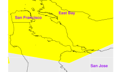
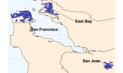
Figure 1: Left: The wildfire smoke coverage on August 31, 2021, where yellow represents exposure to wildfire smoke. Right: The bike share locations in the three outcome units.

Traditional unit-to-unit cross-sectional analyses would be infeasible in our study as it would be impossible to control for attributes of interventional and outcome units, with only three outcome units (see discussion in Section 3.5). However, given daily data on 1,003 days, approximately 140 of which are exposed across the three areas, our approach can be applied to estimate the effect of smoke exposure on each outcome area, without the need to consider location-varying covariates, and controlling for time-varying confounding only.

The matching algorithms balance daily temperature, humidity, and precipitation as potential time-varying confounders, and smooth seasonal trends are balanced implicitly. We find it plausible that no further covariates are necessary beyond weather-related data to meet the unconfoundedness assumptions. This reasoning stems from the understanding that factors influencing wildfire occurrence and smoke dispersion patterns are unlikely to impact biking activity in distant locations. Similarly, economic indices fluctuating over time in outcome areas are probably unrelated to wildfire presence in North American forests.

Table 4 shows the estimates and p-values from Naïve-$t$ and the three matching estimators. The estimate from the naïve approach is positive, implying that smoke increases biking activity. This unreasonable result is likely due to temporal confounding because most exposed time periods occur during the late summer and fall months, while the naïve uses all time periods. Instead, the matching estimators estimate that smoke exposure reduces biking activity in San Francisco, while riding behavior in East Bay and San Jose, are not influenced by wildfire smoke exposure. The matching algorithms use unexposed time periods during the summer and fall months only as matches (see Supplement E.2 for an illustration). These results are statistically significant at the 0.05 level for San Francisco under Matching 1-1, or 1-1/2. Since exposure is relatively dense during the summer and fall months, Matching 1-2 returns approximately half the number of matches compared to the other two matching algorithms, which might explain larger p-values for this estimator.

Table 4: The effect of wildfire smoke on bikeshare hours in San Francisco, East Bay, and San Jose for Naïve-$t$ and the matching estimators. For each region, the three columns correspond to estimate, p-value (bold font if below 0.05), and number of matches.

	San Francisco			East Bay			San Jose
Naïve-$t$	0.973	(1.000)		0.110	(1.000)		0.022	(0.810)
Maching 1-1	-0.553	(0.021)	101	-0.035	(0.239)	103	-0.038	(0.084)	100
Matching 1-1/2	-0.569	(0.018)	101	-0.006	(0.434)	103	-0.031	(0.107)	100
Matching 1-2	-0.253	(0.163)	56	-0.006	(0.448)	59	0.000	(0.501)	59

6 Discussion

In this manuscript we developed a causal inference framework based for time series data with bipartite interference and a random network. We showed that, when focusing on estimands that average over time, controlling for time-varying information allows us to attribute differences in outcomes to causal effects of the exposure. We introduce three algorithms for matching exposed and unexposed time periods, and corresponding matching estimators, which perform well across various complicating scenarios.

Despite the merits of the proposed framework, several open questions remain. In certain applications it would be important to allow for potential outcomes to depend on previous exposures (Bojinov and Shephard, 2019). A careful consideration of the necessary assumptions and approach for estimation in this setting remains to be addressed in future research. Moreover, definition of effects and estimation methods under more complicated exposure mappings in the time series setting persists as an open question. Towards that front, future work could investigate the relative merits of matching, outcome modeling, and weighting approaches within the context of time series data with bipartite interference.

Supplementary information for
“Bipartite causal inference with interference, time series data, and a random network”
by Zhaoyan Song and Georgia Papadogeorgou

Appendix A Theoretical results

A.1 Proof of exposure unconfoundedness

Proof of Proposition 1.

First, since $\bm{X}^{*},\bm{W}^{*},\bm{P}^{*}$ are time-invariant, we can treat them as constants in the condition and thus omit them for simplicity. Next, under 2:

$$P( E_{tj}=e|\mathcal{Y}_{tj}(\cdot),f(t),\bm{W}_{tj},\bm{X}_{t},\bm{P}_{t.j.})$$

$$=\sum_{\forall\bm{g},\bm{a}}P(E_{tj}=e|\bm{G}_{\cdot tj}=\bm{g},\bm{A}_{t}=\bm{a},\mathcal{Y}_{tj}(\cdot),f(t),\bm{W}_{tj},\bm{X}_{t},\bm{P}_{t.j.})\cdot$$

$$\qquad\qquad P(\bm{G}_{\cdot tj}=\bm{g}|\bm{A}_{t}=\bm{a},\mathcal{Y}_{tj}(\cdot),f(t),\bm{W}_{tj},\bm{X}_{t},\bm{P}_{t.j.})\cdot$$

$$\qquad\qquad\qquad P(\bm{A}_{t}=\bm{a}|\mathcal{Y}_{tj}(\cdot),f(t),\bm{W}_{tj},\bm{X}_{t},\bm{P}_{t.j.})$$

$$=\sum_{\forall\bm{g},\bm{a}}I\left(h_{tj}(\bm{a},\bm{g})=e\right)P(\bm{G}_{\cdot tj}=\bm{g}|\bm{A}_{t}=\bm{a},f(t),\bm{W}_{tj},\bm{X}_{t},\bm{P}_{t.j.})P(\bm{A}_{t}=\bm{a}|f(t),\bm{W}_{tj},\bm{X}_{t},\bm{P}_{t.j.})$$

The first equality holds because of the law of total probability and the conditional probability formula. The first component in the second equality is simply the indicator function of the exposure vector equivalent to a known vector or not; the second utilizes Assumption 3 and the third applies Assumption 2. ∎

A.2 Proofs of bias bounds

Proof of Theorem 1.

We consider the case of bounding the bias of the matching algorithms when the outcome model has a linear form in the exposure and time. Define $I_{1}$ as the set of $(t_{tr},t_{c})$ and $I_{2}$ as the set of $(t_{tr},t_{c1},t_{c2})$ as the solution of matched units to the mixed integer programming.

• Matching 1-1

  $$|\operatorname{E}(\widehat{\tau}-\tau)|=$$

  $$=\left|\operatorname{E}\left(\operatorname{E}\left(\frac{1}{|I_{1}|}\sum_{(t_{tr},t_{c})\in I_{1}}Y_{t_{tr}}-Y_{t_{c}}\right)-\left.\left(\frac{1}{|\mathcal{T}_{tr}|}\sum_{t_{tr\in\mathcal{T}_{tr}}}Y_{t_{tr}}(1)-Y_{t_{tr}}(0)\right)\right|\bm{E},\bm{t},\bm{W},\bm{X},\bm{P}\right)\right|$$

  $$=\left|\frac{1}{|I_{1}|}\sum_{(t_{tr},t_{c})\in I_{1}}\left(\beta_{1}+\beta_{2}t_{tr}-\beta_{2}t_{c}+\bm{\beta}_{3}^{\top}\bm{W}_{t_{tr}}-\bm{\beta}_{3}^{\top}\bm{W}_{t_{c}}+\bm{\beta}_{4}^{\top}\widetilde{\bm{X}}_{t_{tr}}-\bm{\beta}_{4}^{\top}\widetilde{\bm{X}}_{t_{c}}+\bm{\beta}_{5}^{\top}\widetilde{\bm{P}}_{t_{tr}}-\bm{\beta}_{5}^{\top}\widetilde{\bm{P}}_{t_{c}}\right)-\beta_{1}\right|$$

  $$\leq\frac{1}{|I_{1}|}|\beta_{2}|\left|\sum_{(t_{tr},t_{c})\in I_{1}}(t_{tr}-t_{c})\right|+\frac{1}{|I_{1}|}\left|\sum_{s}\beta_{3s}\sum_{(t_{tr},t_{c})\in I_{1}}({{W}}_{t_{tr}s}-{{W}}_{t_{c}s})\right|+$$

  $$\qquad\qquad\frac{1}{|I_{1}|}\left|\sum_{s}\beta_{4s}\sum_{(t_{tr},t_{c})\in I_{1}}(\widetilde{X}_{t_{tr}s}-\widetilde{X}_{t_{c}s})\right|+\frac{1}{|I_{1}|}\left|\sum_{s}\beta_{5s}\sum_{(t_{tr},t_{c})\in I_{1}}(\widetilde{P}_{t_{tr}s}-\widetilde{P}_{t_{c}s})\right|$$

  $$<\delta|\beta_{2}|+\delta^{\prime}(\|\bm{\beta}_{3}\|_{1}+\|\bm{\beta}_{4}\|_{1}+\|\bm{\beta}_{5}\|_{1}).$$

• Matching 1-2

  $$|\operatorname{E}(\widehat{\tau}-\tau)|=$$

  $$=\left|\operatorname{E}\left(\operatorname{E}\left(\frac{1}{|I_{2}|}\sum_{(t_{tr},t_{c_{1}},t_{c_{2}})\in I_{2}}Y_{t_{tr}}-\frac{1}{2}(Y_{t_{c_{1}}}+Y_{t_{c_{2}}})\right)-\left.\left(\frac{1}{|\mathcal{T}_{tr}|}\sum_{t_{tr\in\mathcal{T}_{tr}}}Y_{t_{tr}}(1)-Y_{t_{tr}}(0)\right)\right|\bm{E},\bm{t},\bm{W},\bm{X},\bm{P}\right)\right|$$

  $$=\left.\sum_{(t_{tr},t_{c_{1}},t_{c_{2}})\in I_{2}}\left(\beta_{1}+\beta_{2}t_{tr}-\frac{\beta_{2}}{2}(t_{c_{1}}+t_{c_{2}})+\bm{\beta}_{3}^{\top}\bm{W}_{t_{tr}}-\frac{\bm{\beta}_{3}^{\top}}{2}(\bm{W}_{t_{c_{1}}}+\bm{W}_{t_{c_{2}}})+\right.\right.$$

  $$\qquad\quad\left.\left.\bm{\beta}_{4}^{\top}\widetilde{\bm{X}}_{t_{tr}}-\frac{\bm{\beta}_{4}^{\top}}{2}(\widetilde{\bm{X}}_{t_{c_{1}}}+\widetilde{\bm{X}}_{t_{c_{2}}})+\bm{\beta}_{5}^{\top}\widetilde{\bm{P}}_{t_{tr}}-\frac{\bm{\beta}_{5}^{\top}}{2}(\widetilde{\bm{P}}_{t_{c_{1}}}+\widetilde{\bm{P}}_{t_{c_{2}}})\right)-\beta_{1}\right|$$

  $$\leq\frac{1}{|I_{2}|}|\beta_{2}|\left|\sum_{(t_{tr},t_{c_{1}},t_{c_{2}})\in I_{2}}\left(t_{tr}-\frac{1}{2}(t_{c_{1}}+t_{c_{2}})\right)\right|+\frac{1}{|I_{2}|}\left|\sum_{s}\beta_{3s}\sum_{(t_{tr},t_{c_{1}},t_{c_{2}})\in I_{2}}{{W}}_{t_{tr}s}-\frac{1}{2}({{W}}_{t_{c_{1}}s}+{{W}}_{t_{c_{2}}s})\right|+\cdots$$

  $$<\delta|\beta_{2}|+\delta^{\prime}(\|\bm{\beta}_{3}\|_{1}+\|\bm{\beta}_{4}\|_{1}+\|\bm{\beta}_{5}\|_{1}).$$

• Matching 1-1/2

  $$|\operatorname{E}(\widehat{\tau}-\tau)|$$

  $$=\left|\operatorname{E}\left(\operatorname{E}\left(\frac{1}{|I|}\sum_{(t_{tr},t_{c})\in I_{1}}\left(Y_{t_{tr}}-Y_{t_{c}}\right)+\sum_{(t_{tr},t_{c_{1}},t_{c_{2}})\in I_{2}}\left(Y_{t_{tr}}-\frac{1}{2}(Y_{t_{c_{1}}}+Y_{t_{c_{2}}})\right)\right)-\right.\right.$$

  $$\left.\left.\hskip 40.0pt-\left.\left(\frac{1}{|I|}\sum_{j\in I}Y_{t_{tr}}(1)-Y_{t_{tr}}(0)\right)\right|\bm{E},\bm{t},\bm{W},\bm{X},\bm{P}\right)\right|$$

  $$=\left|\frac{1}{|I|}\sum_{(t_{tr},t_{c})\in I_{1}}\left(\beta_{1}+\beta_{2}t_{tr}-\beta_{2}t_{c}+\bm{\beta}_{3}^{\top}\bm{W}_{t_{tr}}-\bm{\beta}_{3}^{\top}\bm{W}_{t_{c}}+\bm{\beta}_{4}^{\top}\widetilde{\bm{X}}_{t_{tr}}-\bm{\beta}_{4}^{\top}\widetilde{\bm{X}}_{t_{c}}+\bm{\beta}_{5}^{\top}\widetilde{\bm{P}}_{t_{tr}}-\bm{\beta}_{5}^{\top}\widetilde{\bm{P}}_{t_{c}}\right)+\right.$$

  $$\qquad\left.\sum_{(t_{tr},t_{c_{1}},t_{c_{2}})\in I_{2}}\left(\beta_{1}+\beta_{2}t_{tr}-\frac{\beta_{2}}{2}(t_{c_{1}}+t_{c_{2}})+\bm{\beta}_{3}^{\top}\bm{W}_{t_{tr}}-\frac{\bm{\beta}_{3}^{\top}}{2}(\bm{W}_{t_{c_{1}}}+\bm{W}_{t_{c_{2}}})+\right.\right.$$

  $$\qquad\quad\left.\left.+\bm{\beta}_{4}^{\top}\widetilde{\bm{X}}_{t_{tr}}-\frac{\bm{\beta}_{4}^{\top}}{2}(\widetilde{\bm{X}}_{t_{c_{1}}}+\widetilde{\bm{X}}_{t_{c_{2}}})+\bm{\beta}_{5}^{\top}\widetilde{\bm{P}}_{t_{tr}}-\frac{\bm{\beta}_{5}^{\top}}{2}(\widetilde{\bm{P}}_{t_{c_{1}}}+\widetilde{\bm{P}}_{t_{c_{2}}})\right)-\beta_{1}\right|$$

  $$\leq\frac{1}{|I|}|\beta_{2}|\left|\sum_{(t_{tr},t_{c})\in I_{1}}(t_{tr}-t_{c})+\sum_{(t_{tr},t_{c_{1}},t_{c_{2}})\in I_{2}}\left(t_{tr}-\frac{1}{2}(t_{c_{1}}+t_{c_{2}})\right)\right|+$$

  $$\qquad\frac{1}{|I|}\left|\sum_{s}\beta_{3s}\left(\sum_{(t_{tr},t_{c})\in I_{1}}W_{t_{tr}s}-W_{t_{c}s}+\sum_{(t_{tr},t_{c_{1}},t_{c_{2}})\in I_{2}}W_{t_{tr}}-\frac{1}{2}(W_{t_{c_{1}}s}+W_{t_{c_{2}}s})\right)\right|+\cdots$$

  $$<\delta|\beta_{2}|+\delta^{\prime}(\|\bm{\beta}_{3}\|_{1}+\|\bm{\beta}_{4}\|_{1}+\|\bm{\beta}_{5}\|_{1}).$$

∎

Proof of Theorem 2.

We study the bias of the matching estimator based on Matching 1-1. The bias bounds of estimators based on Matching 1-2 and Matching 1-1/2 are derived similarly, and therefore are omitted here.

We bound the quantity $h_{s}(W_{t_{tr}s})-h_{s}(W_{t_{c}s})$ below, and similar bounds can be acquired for the functions $h_{s}$ that correspond to $\widetilde{\bm{X}}$ and $\widetilde{\bm{P}}$.

$$\left|\sum_{(t_{tr},t_{c})\in I_{1}}h_{s}(W_{t_{tr}s})-h_{s}(W_{t_{c}s})\right|=$$

$$=\left|\sum_{r=1}^{(b-a)/\ell}\sum_{(t_{tr},t_{c})\in I_{1}}(\sum_{k=1}^{K-1}\gamma_{k}{W}_{t_{tr}sr}^{k\dagger}+R_{t_{tr},r,K})-(\sum_{k=1}^{K-1}\gamma_{k}{W}_{t_{c}sr}^{k\dagger}+R_{t_{c},r,K})\right|$$

$$\leq\sum_{r=1}^{(b-a)/\ell}\left(\sum_{k=1}^{K-1}|\gamma_{k}|\left|\sum_{(t_{tr},t_{c})\in I_{1}}{W}_{t_{tr}sr}^{k\dagger}-{W}_{t_{c}sr}^{k\dagger}\right|+2|I_{1}|\frac{|h_{5}^{(K)|}(\xi_{sr})}{K!}(\ell/2)^{K}\right).$$

$$\leq|I_{1}|\left(\sum_{r=1}^{(b-a)/\ell}(\sum_{k=1}^{K-1}\delta^{\prime}|\gamma_{k}|+2\frac{|h_{s}^{(K)}(\xi_{sr})|}{K!}(\ell/2)^{K})\right)$$

$$\leq|I_{1}|\left((b_{s}-a_{s})/\ell(\sum_{k=1}^{K-1}\delta^{\prime}c/k!+2\frac{c}{K!}(\ell/2)^{K})\right),$$

where $\gamma_{k}:=\frac{h_{s}^{(k)}(\xi_{sr})}{k!}\leq\frac{c}{k!}$ is the coefficient of the Taylor expansion of order $k$ around $\xi_{sr}$, and $R_{t,r,k}$ is the residual of Taylor expansion such that $|R_{t,r,k}|\leq\frac{|h_{s}^{(K)|}(\xi_{sr})}{K!}(\ell/2)^{K}\leq\frac{c}{K!}(\ell/2)^{K}.$ Therefore, we can show

$$|\operatorname{E}(\widehat{\tau}-\tau)|=$$

$$=\left|\operatorname{E}\left(\operatorname{E}\left(\frac{1}{|I_{1}|}\sum_{(t_{tr},t_{c})\in I_{1}}Y_{t_{tr}}-Y_{t_{c}}\right)-\left.\left(\frac{1}{|\mathcal{T}_{tr}|}\sum_{t_{tr\in\mathcal{T}_{tr}}}Y_{t_{tr}}(1)-Y_{t_{tr}}(0)\right)\right|\bm{E},\bm{t},\bm{W},\bm{X},\bm{P}\right)\right|$$

$$=\left|\frac{1}{|I_{1}|}\sum_{(t_{tr},t_{c})\in I_{1}}\left(\theta+\beta+(h_{0}(t_{tr})-h_{0}(t_{c}))+{\scriptstyle\sum\limits_{s=1}^{p_{W}}}(h_{s}(W_{t_{tr}s})-h_{s}(W_{t_{c}s}))+\right.\right.$$

$$\left.\left.\qquad\qquad{\scriptstyle\sum\limits_{s=1}^{p_{X}}}(h_{p_{W}+s}(\widetilde{X}_{t_{tr}s}-h_{p_{W}+s}(\widetilde{X}_{t_{c}s}))+{\scriptstyle\sum\limits_{s=1}^{p_{P}}}(h_{p_{W}+p_{X}+s}(\widetilde{P}_{t_{tr}s})-h_{p_{W}+p_{X}+s}(\widetilde{P}_{t_{c}s}))\right)-\beta_{1}\right|$$

$$\leq\left((T-1)/\ell(\sum_{k=1}^{K-1}\delta c/k!+2\frac{c}{K!}(\ell/2)^{K})\right)+\sum_{s}\left((b_{s}-a_{s})/\ell(\sum_{k=1}^{K-1}\delta^{\prime}c/k!+2\frac{c}{K!}(\ell/2)^{K})\right)$$

$$\leq C_{T}\delta+C_{WXP}\delta^{\prime}+C_{TWXP}\ell^{K-1}.$$

∎

A.3 The bounding constants in Theorem 2

Although we match discrete time periods, we think of the smooth temporal trend as a continuous function for time over the whole interval $[0,T]$. For the time-varying covariates, their supports are indexed by their corresponding additive function, which is $[b_{s}-a_{s}]$ for every $h_{s},s=1,2,\cdots,p_{W}+p_{X}+p_{P}$. The constants $C_{T},C_{WXP}$ and $C_{TWXP}$ are equal to

$$C_{T}=\sum_{k=1}^{K-1}\frac{(T-1)c}{\ell k!},$$

$$C_{WXP}=\sum_{s=1}^{p_{W}+p_{X}+p_{P}}\sum_{k=1}^{K-1}\frac{(b_{s}-a_{s})c}{\ell k!},$$

$$C_{TWXP}=(\frac{1}{2})^{K-1}\left(\frac{(T-1)c}{K!}+\sum_{s=1}^{p_{W}+p_{X}+p_{P}}\frac{(b_{s}-a_{s})c}{K!}\right).$$

Appendix B A Detailed Simulation Description of Section 4

We consider settings with $N=50$ interventional units and $M=200$ outcome units at randomly generated locations on the $[0,1]\times[0,1]$ square in an $(x,y)$ coordinate system. The locations of the interventional and outcome units are generated in the following manner. For the interventional units, the $x$ coordinates of units 1 to 10, 31 to 40 are generated independently from Uniform$(0,0.5)$, while the $x$ coordinates for the remaining units are generated from a Uniform$(0.5,1)$ distribution. The $y$ coordinates for the interventional units are generated from a Uniform$(0,0.5)$ distribution for units 1 to 10 and 21 to 30, and from Uniform$(0.5,1)$ distribution for the remaining units. Similarly, for the outcome units, the $x$ coordinates for units 1 to 68 and 113 to 156 are drawn from a Uniform$(0,0.5)$ distribution, while the $x$ coordinates for the remaining outcome units are drawn from a Uniform$(0.5,1)$ distribution. The $y$ coordinates are drawn from Uniform$(0,0.5)$ for units 1 to 50 and 101 to 150, and from Uniform$(0.5,1)$ for the remaining units.

We generate covariates, treatments, graphs, exposures, and outcomes over $T=400$ time periods. We create scenarios with or without different confounders between exposure and outcome.

B.1 The covariates

We consider six covariates for the interventional units, six covariates for the outcome units, and one network covariate. Specifically, the covariates we consider are as follows:

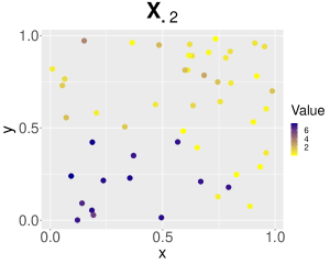
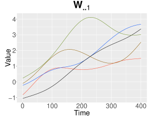
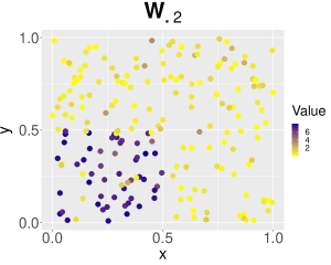
Figure S.2: Visualization of interventional and outcome unit covariates over time and units. The top left panel shows 5 realizations from the Gaussian process for $\bm{X}_{..1}$. The top right figure is the $[0,1]\times[0,1]$ location square with one realization for the location of the interventional points and the corresponding location-varying covariate $\bm{X}_{.2}$. The bottom right figure is 5 realizations from the Gaussian process for $\bm{W}_{..1}$ and the bottom right figure is a realization from the locations of the outcome units colored by the values of one realization of $\bm{W}_{.2}$.

• Interventional unit covariates:

  1. Confounders equal to smooth functions of time: $\bm{X}_{.i1}=({X}_{1i1},X_{2i1},\dots,X_{Ti1})$ is generated from a Gaussian process with Gaussian correlation kernel and mean representing a smooth temporal trend as $\bm{X}_{.i1}\sim\mathcal{N}(f(t),\Sigma)$, where $\Sigma_{t_{1},t_{2}}=\frac{\exp(-({t_{1}}-{t_{2}})^{2})}{2\cdot 100^{2}}$ and $f(t)=\frac{3}{400}t$. Realizations of this covariate $\bm{X}_{.i1}$ for five interventional units is shown on the top-left panel of Figure S.2.

  2. Location-varying confounders: We consider a covariate that varies across unit but not across time, $X_{ti2}=X_{i2}$. For units $i$ inside the $[0,0.5]\times[0,0.5]$ rectangle, we generate $X_{i2}/8\sim$ Beta$(9,1)$; for the rest $i$’s, $X_{i2}/8\sim$ Beta$(1,9)$. A visualization of this covariate for all intervention units is shown at the top-right panel of Figure S.2.

  3. Time-varying confounders: $X_{ti3}\sim{N}(0,t/100),i=1,\cdots,N,t=1,\cdots,T.$ This variable varies across time without a smooth pattern.

• Outcome unit covariates:

  1. Confounders equal to smooth functions of time: $\bm{W}_{.j1}$ is generated by the same Gaussian process as $\bm{X}_{.i1}$, as $\bm{W}_{.j1}\sim{N}(f(t),\Sigma)$, where $\Sigma_{t_{1},t_{2}}=\frac{\exp(-({t_{1}}-{t_{2}})^{2})}{2\cdot 100^{2}}$ and $f(t)=\frac{3}{400}t$. Realizations of this covariate $\bm{W}_{.i1}$ for five outcome units is shown on the bottom-left panel of Figure S.2. It is evident that covariate $\bm{X}_{.i1}$ for the interventional units and covariate $\bm{W}_{.j1}$ for the outcome units represent smooth temporal trends that are similar, but different. Therefore, if $\bm{X}_{.i1}$ is a predictor of the interventional units’ treatment across time, and $\bm{W}_{.j1}$ is a predictor of the outcome units’ outcome across time, then the common smooth temporal trend in $\bm{X}_{.i1}$ and $\bm{W}_{.j1}$ confounds the exposure-outcome relationship of interest.

  2. Location-varying confounders: for units $j$ inside the $[0,0.5]\times[0,0.5]$ square, we let their covariates $W_{tj2}=W_{j2}$, where $W_{j2}/8\sim$ Beta$(9,1)$ for all $t$; for the rest $j$’s, $W_{tj2}=W_{j2}$, where $W_{j2}/8\sim$ Beta$(1,9)$ for all $t$. A visualization of this covariate for all outcome units is shown at the bottom-right panel of Figure S.2. It is evident that the location-varying covariates $\bm{X}_{.2}$ and $\bm{W}_{.2}$ share spatial trends. Therefore, if the former is a predictor of the interventional units’ treatment, and the latter of the outcome units’ outcome, then there exists location-varying confounding of the exposure-outcome relationship.

  3. Time-varying confounders: $W_{tj3}/2\sim$Beta$(t/100,2),j=1,2,\cdots,M,\ t=1,2,\cdots,T.$ This variable has an non-smooth temporal trend.

• Network covariates: We generate $p_{P}=1$ network covariate, and the network covariate array $\bm{P}_{t}$ is an $N\times M$ matrix. The entries of the matrix are generated independently as $P_{tij}\sim$ Beta($t/50,10$), $i=1,2,\cdots,N,\ j=1,2,\cdots,M,\ t=0,1,\cdots,T$. Therefore, the network covariates have a non-smooth temporal trend.

• Bipartite covariates: We consider additional covariates for interventional units based on the weighted average of neighboring outcome unit covariates, and vice versa. We define the $N\times M$ matrix $\bm{R}$, with entries $r_{ij}=1$ if unit $i$ and $j$ are within distance 0.1, and $r_{ij}=0$ otherwise. We set $X_{i4}$ and $\bm{X}_{.i5}$ to denote the $i$th interventional unit-related location and time-varying covariates such that:

  1. $X_{i4}=\frac{\sum_{j}r_{ij}W_{j2}}{\sum_{j}r_{ij}},i=1,2,\cdots,N$, and

  2. $X_{ti5}=\frac{\sum_{j}r_{ij}W_{tj3}}{\sum_{j}r_{ij}},i=1,2,\cdots,N,\ t=1,2,\cdots,T.$

  Similarly we set ${W}_{j4}$ and $\bm{W}_{.j5}$ to denote the $j$th outcome-unit-related location and time-varying covariates. Here, is useful to introduce the matrix $\bm{Q}$, whose columns are the normalized version of the columns of $\bm{R}.$ Specifically, the $(i,j)$th entry is equal to $q_{ij}=r_{ij}/\sum_{i}r_{ij}$. Then, the covariates are defined as

  1. $W_{j4}={\sum_{i}q_{ij}X_{i2}},j=1,2,\cdots,N$, and

  2. $W_{tj5}={\sum_{i}q_{ij}X_{ti3}},j=1,2,\cdots,N,\ t=1,2\cdots,T.$

  The columns of the matrix $\bm{Q}$ correspond to the vectors $\bm{q}$ we introduce in Section 3.1 for defining the interventional and network covariate summaries.

• For every unit, there is an associated time-varying location-invariant confounder, termed $X_{ti6}=W_{tj6}=Z_{t}$, following $\mathcal{N}(t/200,\log(t)/10)$ everywhere.

B.2 The treatment assignment, bipartite network, and outcome

We consider five scenarios regarding the confounding structure. In terms of the treatment assignment, the five scenarios consider the following generation of treatment vectors over the interventional units across time.

1. No confounders:

   $$A_{ti} \sim\text{Uniform}(0,1),$$

   $$G_{tij} \sim\text{Ber}(\rho),\quad\quad\text{where }\rho=0.17,$$

   $$Y_{tj} =E_{tj}+W_{j2}+\epsilon_{tj}.$$

2. Only time-smooth confounders exist:

   $$A_{ti}\mid X_{ti1} \sim\text{Ber}(1/(1+\exp(X_{ti1}/1.2))$$

   $$G_{tij} \sim\text{Ber}(\rho_{ij}),\quad\quad\text{where }\rho_{ij}=1/(2(1+\exp dist(i,j)),$$

   $$Y_{tj} =E_{tj}+W_{tj1}+\epsilon_{tj}$$

3. Only location-varying confounders exist:

   $$A_{ti}\mid X_{i2},X_{i4} \sim\text{Ber}({1}/{(1+0.3\exp{(X_{i2}}-X_{i4}/40))})$$

   $$G_{tij} \sim\text{Ber}(\rho_{ij}),\quad\quad\text{where }\rho_{ij}=1/(1.7(1+\exp dist(i,j))$$

   $$Y_{tj} =E_{tj}+4W_{j2}+4W_{j4}+\epsilon_{tj}$$

4. Only time-varying confounders exist:

   $$A_{ti}\mid X_{ti3},X_{ti5},X_{ti6},\bm{P}_{t} \sim\text{Ber}(\frac{1}{1+\exp(X_{ti3}/2+X_{ti5}/2+X_{ti6}+\sum_{j}r_{ij}P_{tij}/(10\sum_{j}r_{ij}))})$$

   $$G_{tij}\mid t \sim\text{Ber}(\rho_{tij}),\quad\text{where }\rho_{tij}={1}/(1+0.1\exp{\sin(\pi t/1000)}+\exp{dist(i,j)})$$

   $$Y_{tj} =E_{tj}+W_{tj3}+W_{tj5}+{\sum_{i}q_{ij}P_{tij}}+W_{tj6}+\epsilon_{tj}$$

5. All confounders exist:

   $$A_{ti}\mid\bm{X}_{t},\bm{P}_{t}\sim{\text{Ber}(\eta_{tij})},\quad\quad\text{where}$$

   $$\eta_{tij}=\frac{1}{1+0.45\exp(X_{ti1}/20+X_{i2}+X_{ti3}/100+X_{i4}+X_{ti5}/20+X_{ti6}/1.5+\sum_{j}r_{ij}P_{tij}/(10\sum_{j}r_{ij}))}$$

   $$G_{tij}\mid t\sim\text{Ber}(\rho_{tij}),\quad\quad\text{where }\rho_{tij}={1}/(1+0.1\exp{\sin(\pi t/1000)}+\exp{dist(i,j)})$$

   $$Y_{tj}=E_{tj}+W_{tj1}+2*W_{j2}+W_{tj3}+0.1*W_{tj3}^{2}+2*W_{j4}+W_{tj5}+1/(1+\exp(W_{tj5}))+$$

   $$\qquad\qquad\sin\left({\sum_{i}q_{ij}P_{tij}}\right)+2W_{tj6}+\epsilon_{tj}$$

Appendix C Description for naïve approaches

Implementing three naïve approaches requires a full dataset including exposure status $E_{tj}$ and outcomes $Y_{tj}$ among all units $m_{1},m_{2},\cdots,m_{M}$ and all time points $t=1,2,\cdots,T$. While Naïve-uses the full dataset, Naïve-$t$ uses only the data from the first outcome unit across time, and Naïve-$j$ uses the data across all outcome units but only for the first time point.

C.1 Estimator

For Naïve-$t$, we split the temporal data for the first outcome unit into two groups: the exposed time periods, $t\in\mathcal{T}_{tr}$ if $E_{jt}=1$, and the unexposed time periods, $t\in\mathcal{T}_{c}$. Similarly for Naïve-$j$, we split the data for the outcome units in the exposed outcome units, $j\in\mathcal{J}_{tr}$ if $E_{jt}=1$, and the unexposed outcome units, $j\in\mathcal{J}_{c}$ otherwise. For Naïve-all, the tuple $(t,j)\in\mathcal{S}_{tr}$ if $E_{jt}=1$ and $(t,j)\in\mathcal{S}_{c}$ otherwise. We use the estimators $\widehat{\tau}^{\text{Na\"{i}ve}-t},\widehat{\tau}^{\text{Na\"{i}ve}-j}$ and $\widehat{\tau}^{\text{Na\"{i}ve}-all}$as follows:

$$\widehat{\tau}^{\text{Na\"{i}ve}-t} =\frac{1}{|\mathcal{T}_{tr}|}\sum_{t\in\mathcal{T}_{tr}}Y_{tj}-\frac{1}{|\mathcal{T}_{c}|}\sum_{t\in\mathcal{T}_{c}}Y_{tj},$$

$$\widehat{\tau}^{\text{Na\"{i}ve}-j} =\frac{1}{|\mathcal{J}_{tr}|}\sum_{j\in\mathcal{J}_{tr}}Y_{tj}-\frac{1}{|\mathcal{J}_{c}|}\sum_{j\in\mathcal{J}_{c}}Y_{tj},$$

$$\widehat{\tau}^{\text{Na\"{i}ve}-all} =\frac{1}{|\mathcal{S}_{tr}|}\sum_{(t,j)\in\mathcal{S}_{tr}}Y_{tj}-\frac{1}{|\mathcal{S}_{c}|}\sum_{(t,j)\in\mathcal{S}_{c}}Y_{tj}.$$

C.2 Inference

We adopted the classic Wald-type confidence interval construction for two independent samples. Denote $s_{tr}$ as the standard deviation of outcomes with index from $\mathcal{T}_{tr},\mathcal{J}_{tr}$ or $\mathcal{S}_{tr}$, and $s_{c}$ as the standard deviation of outcomes with index from $\mathcal{T}_{c},\mathcal{J}_{c}$ or $\mathcal{S}_{c}$ for each naïve approach. The confidence intervals for Naïve-$t$, Naïve-$j$, and Naïve-all are

$$\widehat{\tau}^{\text{Na\"{i}ve}-t}\pm Z_{\alpha}\sqrt{\frac{(|\mathcal{T}_{tr}|-1)s_{tr}^{2}+(|\mathcal{T}_{c}|-1)s_{c}^{2}}{|\mathcal{T}_{tr}|+|\mathcal{T}_{c}|-2}}\sqrt{\frac{1}{|\mathcal{T}_{tr}|}+\frac{1}{|\mathcal{T}_{c}|}},$$

$$\widehat{\tau}^{\text{Na\"{i}ve}-j}\pm Z_{\alpha}\sqrt{\frac{(|\mathcal{J}_{tr}|-1)s_{tr}^{2}+(|\mathcal{J}_{c}|-1)s_{c}^{2}}{|\mathcal{J}_{tr}|+|\mathcal{J}_{c}|-2}}\sqrt{\frac{1}{|\mathcal{J}_{tr}|}+\frac{1}{|\mathcal{J}_{c}|}},$$

and

$$\widehat{\tau}^{\text{Na\"{i}ve}-all}\pm Z_{\alpha}\sqrt{\frac{(|\mathcal{S}_{tr}|-1)s_{tr}^{2}+(|\mathcal{S}_{c}|-1)s_{c}^{2}}{|\mathcal{S}_{tr}|+|\mathcal{S}_{c}|-2}}\sqrt{\frac{1}{|\mathcal{S}_{tr}|}+\frac{1}{|\mathcal{S}_{c}|}},$$

respectively.

Appendix D Additional Simulation Results

D.1 Unadjusted matching

We state the methodology for unadjusted matching with time series data given exposure and outcome values at each time period. For the three matching criteria, 1-1, 1-2, and 1-1/2, we balance time but not the time-varying confounders. Specifically, we remove constraints (A.4)-(A.6) for 1-1 objective (A), (B.6)-(B.8) for 1-2 objective (B), and (C.6)-(C.8) for 1-1/2 objective (C).

We evaluate the performance of the unadjusted estimator in the simulations of Section 4. In Table S.5 we show the bias, mean squared error, coverage, and proportion of matched exposure when applying three unadjusted matching algorithms. Unadjusted matching estimators are unbiased with nominal coverage in the absence of non-smooth time-varying confounders, even in the presence of confounding temporal trends, in cases (a), (b) and (c). However, in the scenarios with non-smooth time-varying confounding, unadjusted estimators will be biased. The proportion of exposed time points that are matched using unadjusted approaches is only slightly higher than the proportion for adjusted approaches in some scenarios.

Table S.5: Simulation results of single-unit estimations. Bias, mean squared error (MSE), coverage of 95% intervals (%), and proportion of exposed time points being matched (%). We show simulation results for 3 unadjusted matching methods. ‘U’ stands for ‘unadjusted’.

		Dense				Medium				Sparse
	Method	Bias	MSE	Cover	Prop	Bias	MSE	Cover	Prop	Bias	MSE	Cover	Prop
(a)1	U1-1	-0.00	0.011	96.4	97.8	-0.00	0.020	94.8	100.0	-0.00	0.039	95.0	100.0
	U1-1/2	-0.00	0.011	94.8	97.8	-0.00	0.018	95.0	100.0	-0.01	0.036	95.4	100.0
	U1-2	-0.01	0.014	94.6	62.2	-0.01	0.016	95.6	90.8	-0.01	0.031	93.2	98.8
(b)1	U1-1	-0.00	0.019	95.2	62.7	-0.00	0.025	93.8	85.1	0.00	0.036	95.8	97.7
	U1-1/2	0.00	0.020	94.8	62.7	-0.00	0.022	94.6	85.1	0.00	0.033	94.0	97.7
	U1-2	-0.01	0.023	94.8	41.1	0.00	0.025	93.4	59.9	0.00	0.035	94.8	80.5
(c)1	U1-1	-0.01	0.013	94.4	91.1	0.00	0.020	94.2	99.7	0.01	0.040	93.8	100.0
	U1-1/2	-0.01	0.013	94.4	91.1	-0.00	0.017	94.2	99.7	0.00	0.039	94.2	100.0
	U1-2	-0.01	0.017	93.0	56.4	0.00	0.017	93.8	85.6	-0.00	0.029	92.8	97.4
(d)1	U1-1	-0.4	0.226	55.0	69.8	-0.37	0.192	59.4	86.2	-0.35	0.218	80.0	99.8
	U1-1/2	-0.41	0.225	48.4	69.8	-0.37	0.190	57.4	86.2	-0.36	0.223	75.0	99.8
	U1-2	-0.44	0.278	53.4	47.1	-0.42	0.234	57.6	63.2	-0.35	0.206	77.2	92.0
(e)1	U1-1	-0.64	0.477	23.3	76.4	-0.60	0.429	30.0	95.0	-0.61	0.480	53.6	99.7
	U1-1/2	-0.63	0.450	20.3	76.4	-0.59	0.416	34.6	95.0	-0.60	0.462	47.8	99.7
	U1-2	-0.67	0.520	27.4	51.4	-0.64	0.484	30.4	74.7	-0.62	0.484	45.2	91.5

• ¹The scenarios shown in Table S.5 correspond to (a) No confounders, (b) Time-smooth confounders, (c) Location-varying confounders, (d) Time-varying confounders, and (e) All confounders.

We also demonstrated the performance of unadjusted matching under multiple hypothesis simulations in Section 4.2.2. The results are shown in Table S.6. The unadjusted methods give reliable inferences for testing the global null in the absence of confounders or in the presence of only time-smooth confounders.

Table S.6: Simulation results for using 3 unadjusted matching methods to test the global null hypothesis for scenarios (b), (d) and (e), and under a medium exposure level. ‘U’ stands for ‘unadjusted’.

		Average estimator mean	Average rate of p-value $\leq$ 0.05	Rate of min(p-value) $\leq$ 0.05	Rate of FDR min (adj.p-value) $\leq$ 0.05
(b)	U1-1	-0.00	0.053	1.000	0.078
	U1-1/2	-0.00	0.052	1.000	0.103
	U1-2	-0.00	0.055	1.000	0.109
(d)	U1-1	-0.39	0.422	1.000	0.996
	U1-1/2	-0.39	0.445	1.000	0.996
	U1-2	-0.43	0.437	1.000	0.998
(e)	U1-1	-0.62	0.720	1.000	1.000
	U1-1/2	-0.62	0.748	1.000	1.000
	U1-2	-0.67	0.735	1.000	1.000

D.2 Analysis of tuning parameters

Following the simulation study in Section 4.1.2, we apply two different sets of $(\delta,\delta^{\prime},\epsilon)$ per simulation: $(0,0.01,2)$ and $(2,0.05,6)$. In Table S.7, we compare the performance of tuning either $(\delta,\epsilon)$ that correspond to tuning parameters of time, or $\delta^{\prime}$ that is a tuning parameter for the measured covariates in comparison to the default setting $(\delta,\delta^{\prime},\epsilon)=(2,0.01,6)$ (which is shown in Table 2).

Some conclusions from this comparison are discussed in Section 4.2.3. Here, we also point out that, even though Matching 1-2 performed best under sparse scenarios in Table 2, when $(\delta,\epsilon)$ are small, Matching 1-2 is no longer best. That is because the tight constraints exclude many possible 1-2 pairs, and the proportion of exposed time points that are matched is almost half of that of 1-1 or 1-1/2 matching strategies, resulting in large variability for the matching 1-2 estimator.

Table S.7: Simulation results of single-unit estimations under different tuning parameters.

		Dense				Medium				Sparse
Method		Bias	MSE	Cover	Prop	Bias	MSE	Cover	Prop	Bias	MSE	Cover	Prop
No confounders
1-1	$(1)^{1}$	-0.00	0.01	93.8	87.1	-0.01	0.02	94.8	98.3	-0.00	0.04	94.4	99.9
	(2)	-0.00	0.01	94.0	97.8	-0.00	0.02	95.6	100.0	-0.00	0.04	95.4	100.0
	(3)	-0.00	0.01	95.0	97.8	-0.01	0.02	95.2	100.0	-0.01	0.04	94.4	100.0
1-1/2	(1)	0.00	0.01	95.2	87.1	-0.01	0.02	95.0	98.3	-0.01	0.03	95.4	99.9
	(2)	-0.00	0.01	95.0	97.8	-0.00	0.02	95.2	100.0	-0.00	0.03	96.0	100.0
	(3)	-0.00	0.01	94.4	97.8	-0.00	0.02	95.8	100.0	-0.01	0.03	94.8	100.0
1-2	(1)	-0.01	0.02	96.0	40.7	0.00	0.02	94.4	63.9	-0.01	0.04	93.2	81.7
	(2)	-0.01	0.01	96.2	62.2	-0.01	0.02	95.0	90.8	-0.00	0.03	95.0	98.8
	(3)	-0.01	0.01	95.2	62.4	-0.01	0.02	95.8	90.8	-0.01	0.03	96.0	98.7
Time-smooth confounders
1-1	(1)	0.01	0.02	94.8	58.2	0.00	0.03	94.8	78.7	0.02	0.04	93.0	93.1
	(2)	-0.00	0.02	95.4	62.7	-0.00	0.02	93.0	85.1	0.00	0.04	94.6	97.7
	(3)	-0.00	0.02	94.2	62.5	-0.00	0.02	94.4	85.1	0.01	0.04	96.2	97.8
1-1/2	(1)	0.01	0.02	95.2	58.2	0.01	0.02	95.6	78.7	0.02	0.04	95.2	93.2
	(2)	-0.01	0.02	94.4	62.7	-0.00	0.02	95.4	85.1	0.01	0.03	95.2	97.7
	(3)	-0.01	0.02	93.6	62.5	-0.01	0.02	94.6	85.1	0.01	0.03	94.4	97.8
1-2	(1)	0.01	0.03	94.4	28.3	0.01	0.04	92.6	42.9	0.02	0.05	94.2	59.0
	(2)	-0.00	0.02	95.6	41.1	0.01	0.02	95.0	59.9	0.00	0.03	95.0	80.5
	(3)	-0.01	0.02	95.0	40.9	0.00	0.03	94.4	59.9	0.00	0.03	95.0	80.6
Location-varying confounders
1-1	(1)	-0.01	0.01	93.6	80.9	-0.00	0.02	94.2	96.3	0.01	0.04	94.6	99.6
	(2)	-0.01	0.01	94.8	91.1	0.00	0.02	94.2	99.7	0.00	0.04	95.2	100.0
	(3)	-0.01	0.01	94.4	91.1	0.01	0.02	95.4	99.7	0.01	0.04	95.4	100.0
1-1/2	(1)	-0.01	0.01	94.2	80.9	-0.00	0.02	94.4	96.3	0.01	0.04	94.4	99.6
	(2)	-0.01	0.01	95.2	91.1	0.00	0.02	93.6	99.7	-0.00	0.03	94.6	100.0
	(3)	-0.01	0.01	94.0	91.1	0.00	0.02	95.2	99.7	0.01	0.03	95.8	100.0
1-2	(1)	-0.00	0.03	93.4	36.6	0.01	0.03	93.2	59.8	0.01	0.04	95.8	78.6
	(2)	-0.01	0.02	95.6	56.4	-0.00	0.02	94.0	85.6	0.00	0.03	93.8	97.4
	(3)	-0.01	0.02	94.8	56.4	0.00	0.02	94.6	85.6	0.00	0.03	93.6	97.3
Time-varying confounders
1-1	(1)	-0.01	0.02	98.8	57.8	-0.01	0.02	99.0	73.3	-0.02	0.06	97.2	90.3
	(2)	-0.00	0.02	98.4	67.3	-0.02	0.02	98.6	84.4	-0.02	0.06	97.0	99.6
	(3)	-0.06	0.02	98.4	68.4	-0.06	0.02	97.6	85.4	-0.04	0.06	95.6	99.8
1-1/2	(1)	-0.00	0.02	98.8	57.8	-0.01	0.02	99.0	73.3	-0.02	0.06	97.8	90.5
	(2)	-0.00	0.02	98.0	67.3	-0.02	0.02	98.6	84.4	-0.01	0.05	96.8	99.6
	(3)	-0.06	0.02	98.0	68.4	-0.06	0.03	97.0	85.4	-0.04	0.05	95.2	99.8
1-2	(1)	0.00	0.03	99.0	26.4	-0.01	0.04	98.4	37.2	-0.01	0.08	97.6	54.8
	(2)	-0.01	0.02	97.8	43.0	-0.01	0.02	97.0	58.4	-0.02	0.05	96.4	86.2
	(3)	-0.06	0.03	98.2	44.3	-0.06	0.03	97.4	60.2	-0.05	0.05	96.0	88.8
All confounders
1-1	(1)	-0.02	0.02	99.2	64.7	-0.02	0.03	99.6	83.7	-0.00	0.05	99.0	92.3
	(2)	-0.02	0.02	98.7	74.9	-0.01	0.03	98.4	94.2	0.00	0.04	99.4	99.6
	(3)	-0.1	0.03	97.2	75.8	-0.09	0.04	96.6	94.4	-0.06	0.05	99.0	99.7
1-1/2	(1)	-0.02	0.02	99.0	64.8	-0.02	0.03	99.4	83.8	0.01	0.05	99.0	92.5
	(2)	-0.02	0.02	98.3	74.9	-0.01	0.03	98.4	94.2	0.00	0.04	98.8	99.6
	(3)	-0.11	0.03	96.8	75.8	-0.09	0.04	96.4	94.4	-0.07	0.04	97.8	99.7
1-2	(1)	-0.02	0.03	99.2	30.4	-0.00	0.04	99.4	46.2	0.00	0.06	99.0	57.7
	(2)	-0.02	0.02	99.1	48.6	-0.02	0.03	98.6	70.7	0.00	0.04	98.4	87.2
	(3)	-0.1	0.03	98.4	49.8	-0.1	0.04	97.8	71.8	-0.08	0.04	97.0	89.2

• ¹Tuning parameters: (1) strict: $(\delta,\delta^{\prime},\epsilon)=(0,0.01,2)$, (2) medium: $(\delta,\delta^{\prime},\epsilon)=(2,0.01,6)$ (the results in Table 2 correspond to this choice of tuning parameters), (3) loose: $(\delta,\delta^{\prime},\epsilon)=(2,0.05,6)$.

D.3 Modification of matching methods: Covariate balancing within matches

In Section 4.1.2 we observe coverage of our 95% intervals that is larger than the nominal level. Here, we illustrate that this issue of over-coverage is alleviated when covariate balance is imposed for every match. We extend the matching algorithms in Equation A, Equation B and Equation C to include additional constraints. For simplicity, we only show the constraints for the outcome unit covariates, but similar constrains are adopted for the interventional and network time-varying covariates as well. Given a small value $\delta^{\prime\prime}$, for matching 1-1 in Equation A we impose

$$|a_{t_{tr}t_{c}}(\bm{W}_{t_{tr}}-\bm{W}_{t_{c}})|\leq\bm{1}_{p_{W}}\cdot\delta^{\prime\prime},\quad\forall t_{tr}\in\mathcal{T}_{tr},\forall t_{c}\in\mathcal{T}_{c},$$

and similarly for Matching 1-2 in Equation B we impose

$$\left|a_{t_{tr}t_{c_{1}}t_{c_{2}}}\left(\bm{W}_{t_{tr}}-\frac{\bm{W}_{t{c_{1}}}+\bm{W}_{t{c_{2}}}}{2}\right)\right|\leq\bm{1}_{p_{W}}\cdot\delta^{\prime\prime},\quad\forall t_{tr}\in\mathcal{T}_{tr},\forall t_{c_{1}},t_{c_{2}}\in\mathcal{T}_{c}.$$

We evaluated the performance of these extended matching estimators under confounding scenario (d) with medium sparsity level. We set $\delta^{\prime\prime}=0.5$. As a comparison, the standard deviation of time-varying covariates $\bm{W}_{..3}$, $\bm{W}_{..5}$, $\bm{W}_{..6}$ and $\widetilde{\bm{P}}_{.}$ varies from 0.3 to 1.7. In Figure S.3, we see that the three extended matching estimators are unbiased for the true causal effect (which is equal to 1). The coverage rates for the estimators based on the extended algorithms 1-1, 1-1/2, and 1/2 are 97.4%, 97.4%, and 96.8%, respectively, closer to the nominal level than the coverage rates of the matching estimators that do not balance covariates within each match (included in Table 2 and equal to 98.6%, 98.6% and 97.8% for Matching 1-1, 1-1/2 and 1/2, respectively). We believe that the coverage of the extended estimators remains above 95% due to the relatively large value of $\delta^{\prime\prime}$ we consider, which implies that matched exposed and unexposed time periods can still somewhat with respect to their measured covariates. The proportion of matches is lower for smaller values of $\delta^{\prime\prime}$ which impose stricter balance constraints within each match. Therefore, we did not evaluate the coverage for extended matching estimators that employ smaller values of $\delta^{\prime\prime}$. Even with $\delta^{\prime\prime}=0.5$, the proportion of matched exposed time periods decreases significantly to 60.9%, 69.1%, and 47.5% for Extended 1-1, Extended 1-1/2, and Extended 1-2, respectively. We can conclude that the new matching that incorporates the within-match adjustment has the benefit of coverage that is closer to the nominal level, but suffers from a lower proportion of matched exposed time periods.

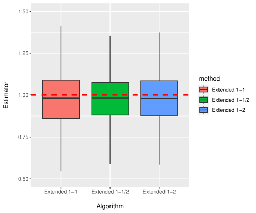
Figure S.3: Boxplots of estimated causal effects over 500 data sets based on the extended estimators.

D.4 Network-outcome confounding can lead to exposure-outcome confounding

We illustrate that confounding of the exposure-outcome relationship can arise due to confounding of the network-outcome relationship, even in the absence of confounding between the interventional units’ treatment and the outcome. To do so, we revisit the no-confounding scenario (a) shown Table 1 and modify the generation of the network to impose network-outcome confounding. Specifically, we generate the entries of G independently as $G_{tij}\sim\text{Ber}(\rho_{ij})$, for $\rho_{ij}=1/(1.7(1+\exp dist(i,j))$. Under this modification, the network G and the outcomes are both associated with location-varying information. We consider the medium sparsity level. Estimated effects are shown in S.4. We see that Naïve-all and Naïve-$j$ are both biased, illustrating that the network-outcome dependence on location-varying information has introduced confounding of the exposure-outcome relationship.

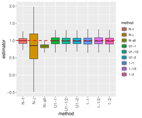
Figure S.4: Boxplots of causal effect estimates for the naïve methods, the matching estimators without adjustment for measured covariates (discussed in Supplement D.1), and the matching estimators with balance constraints for measured covariates. This scenario corresponds to the case with exposure-outcome confounding due to network-outcome dependence on location-varying information.

D.5 Simulations under heterogeneous treatment effects

We performed a simulation where exposure effects are no longer homogeneous over time for an individual outcome unit. We defined three new estimands, termed $\tilde{\tau}^{\mathrm{1-1}}_{j}(e,e^{\prime}),\tilde{\tau}^{\mathrm{1-1/2}}_{j}(e,e^{\prime})$ and $\tilde{\tau}^{\mathrm{1-2}}_{j}(e,e^{\prime})$, as the average difference in potential outcome between exposures $e$ and $e^{\prime}$ over the exposed time periods that are matched according to 1-1, 1-1/2, and 1-2, respectively. For example, $\tilde{\tau}^{\mathrm{1-1}}_{j}(e,e^{\prime})$ can be written as

$$\tilde{\tau}^{\mathrm{1-1}}_{j}(e,e^{\prime})=\frac{1}{\sum_{t:\ \mathrm{matched\ in\ 1-1}}I(E_{tj}=e)}\sum_{t:\ \mathrm{matched\ in\ 1-1}}(Y_{tj}(e)-Y_{tj}(e^{\prime}))I(E_{tj}=e).$$

For ease of notation, in single-unit simulations under binary exposure, we simplify them as $\tilde{\tau}^{\mathrm{1-1}},\tilde{\tau}^{\mathrm{1-1/2}}$ and $\tilde{\tau}^{\mathrm{1-2}}$.

The data generating process is based on scenario (d) under medium exposure. Compared to scenario (d), we alter the generation of the outcome variable to include treatment effects that vary across units and across time. Specifically, we specify

$$Y_{tj}=(1+\epsilon^{\prime}_{tj})E_{tj}+0.005(400-t)E_{tj}+W_{tj3}+W_{tj5}+\sum_{i}q_{ij}P_{tij}+W_{tj6}+\epsilon_{tj},$$

where $\epsilon^{\prime}_{tj}$ are generated independently from $N(0,1).$ We simulate 500 data sets and consider estimation of effects for the first outcome unit.

We compare matching approaches to Naïve-t. We exclude Naïve-$j$ and Naïve-all from simulations under heterogeneity since the estimands they target average across units, whereas Naïve-t and the matching estimators target unit-specific effects.

The bias, MSE, Coverage and proportion of exposed units that are matched are shown in Table S.8. We evaluate the performance of the three matching estimators and Naïve-$t$ for estimating the average effect over all time points $\tau$, and the average effect over all exposed time points $\widetilde{\tau}$. We also evaluate the performance of each matching estimator against the causal effect over the set of exposed time periods that are in fact matched, in that we evaluate the 1-1 matching estimator for estimating $\widetilde{\tau}_{1-1}$, the 1-1/2 matching estimator for estimating $\widetilde{\tau}_{1-1/2}$ and the 1-2 matching estimator for estimating $\widetilde{\tau}_{1-2}$. In the presence of heterogeneous effects across time, the matching estimators perform relatively well for estimating the effect over the exposed $\tilde{\tau}$, and substantially better than the Naïve-$t$ approach that suffers from confounding bias. Particularly, Matching 1-1 and 1-1/2 which match 85% of the exposed time points are close to unbiased with appropriate coverage of confidence intervals. When compared against the effect over the matched exposed population, $\tilde{\tau}^{\mathrm{1-1}},\tilde{\tau}^{\mathrm{1-1/2}}$ and $\tilde{\tau}^{\mathrm{1-2}}$ the estimators are unbiased with appropriate coverage. This suggests that even though the effect of exposure is not constant at each time point, matching approaches can still serve as a useful tool for inferring the average effect of the exposure.

Table S.8: Simulation results under heterogeneous effects for a single outcome unit. Bias, mean squared error (MSE), coverage of 95% intervals (%) of the Naïve-$t$ method and matching methods, and proportion of exposed units being matched of matching methods.

Estimand	Method	Bias	MSE	Coverage	Proportion
$\tau$	Naïve	-0.62	0.44	29.2	-
	1-1	0.40	0.20	60.8	85.1
	1-1/2	0.40	0.20	59.2	85.1
	1-2	0.30	0.14	84.4	59.9
$\widetilde{\tau}$	Naïve	-1.09	1.25	1.4	-
	1-1	-0.07	0.03	98.4	85.1
	1-1/2	-0.07	0.03	97.6	85.1
	1-2	-0.17	0.06	95.2	59.9
$\widetilde{\tau}_{1-1}$	Naïve	-1.02	1.11	2.0	-
	1-1	0.00	0.03	98.8	85.1
$\widetilde{\tau}_{1-2}$	Naïve	-1.02	1.11	2.0	-
	1-2	0.00	0.02	98.8	85.1
$\widetilde{\tau}_{1-1/2}$	Naïve	-0.92	0.91	4.2	-
	1-1/2	0.00	0.03	99.2	59.9

D.6 The impact of temporal correlation in the outcome variable on inference

To analyze the impact of temporal correlation in the outcome variable on coverage, we alter scenario (a) under medium exposure such that the outcome error term $\epsilon$ is equal to $\epsilon_{tj}=\rho\epsilon_{(t-1)j}+\sqrt{1-\rho^{2}}e_{t}$, where $e_{t}\sim N(0,1),$ and $\rho$ is a tuning parameter adjusting the amount of autocorrelation of the error term. We simulate 500 data sets under different levels of autocorrelation, $\rho=0.2,0.4,0.6$ and $0.8$, and recorded the coverage of the three matching estimators. The results are shown in Table S.9. The correlation in the outcome across time has minimal impact on the coverage of the confidence intervals, which is close to 95% across all scenarios, even when auto-correlation in the error term is very high ($\rho=0.8$).

Table S.9: Simulation results of single-unit estimation in the presence of temporal correlation $\rho=0.2,0.4,0.6$ and 0.8 in the random error term. in the outcome variable. Coverage of 95% intervals (%) of matching methods.

$\rho$	1-1	1-1/2	1-2
0.2	98.0	96.0	97.0
0.4	98.0	96.6	96.8
0.6	96.0	96.2	95.8
0.8	95.6	94.2	95.6

Appendix E Additional study information

E.1 Information on data availability and creation

In our study, the interventional units correspond to the different locations of forested area in North America, each of which might experience a wildfire or not. Hazardous smoke produced by wildfires can travel long distances, and affect population exposure and behavior across different areas. The National Oceanic and Atmospheric Administration’s Hazard Mapping System (HMS) combines data from polar and geostationary satellites in real-time, enabling experts to accurately identify and track the dispersion of smoke. The HMS data can be found at https://www.ospo.noaa.gov/Products/land/hms.html, which report daily smoke exposure across the United States as light, medium or high based on smoke thickness.

We focus on three outcome units: San Francisco, San Jose and East Bay in northern California, which might experience exposure to smoke from wildfires or not, based on random patterns of smoke transport and dispersion. Using HMS, we consider an area as exposed if smoke thickness is light or higher. During most of the time periods under study (January 2021 to September 2023), all three regions are either simultaneously exposed or unexposed. Overall, the numbers of wildfire exposed days are 147 for San Francisco, 147 for East Bay and 137 for San Jose. The scenario in Figure 1 where two of the three regions are exposed is rare, but we include it for illustration purposes.

The outcome of interest corresponds to the total daily amount of bicycle riding time using Lyft’s Bay Wheels bikeshare program, which records daily bikeshare usage since 2017 with more than 450 bikeshare stations. This database is available for public use at https://www.lyft.com/bikes/bay-wheels/system-data. We can obtain from it that more than 97% of rides last less than 1 hour, meaning it is unlikely to rent a bike overnight, and rides begin and end within the same area. Therefore, it is reasonable to assume there is little spillover effect across time or outcome units.

Due to the temperature and drought season, there are more wildfires and gusty winds in late summer than in the other seasons. As a result, the exposed time periods and the corresponding matched unexposed ones, concentrate around the late summer and fall (see Supplement E.2). Therefore, the matching algorithms use information on exposed and unexposed time periods during the summer and fall. This is in contrast to the naïve approach, which uses data on all seasons, including the winter months were both exposure and bike activity are expected to be lower.

E.2 Illustrations of matched data for San Francisco

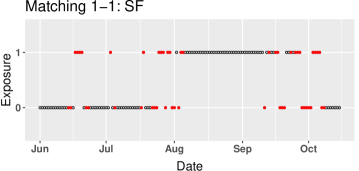
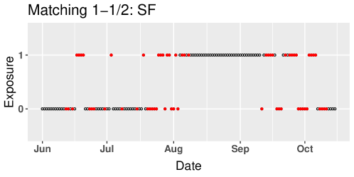
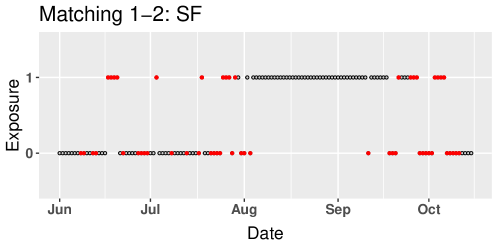
Figure S.5: Exposure and matching information for Matching 1-1, Matching 1-1/2, and Matching 1-2 for San Francisco during the period from June 1, 2021, to October 15, 2021. The hollow dots are time periods that are not matched while the red dots correspond to matched time periods.

We analyze data from January 2021 until September 2023. Most exposed time periods, and as a result most matches, occur during the summer and fall months. As an illustration, the exposed and unexposed time periods for a subset of our time window and for San Francisco are shown in Figure S.5, with red color denoting whether the time period was used in a match according to Matching 1-1, Matching 1-1/2, or Matching 1-2. Under $\epsilon=6$, Matching 1-1 and Matching 1-1/2 have similar but not identical matching patterns, while Matching 1-2 matches fewer exposed time periods.

References

- Abadie and Cattaneo [2018] Alberto Abadie and Matias D Cattaneo. Econometric methods for program evaluation. Annual Review of Economics, 10:465–503, 2018.
- Abadie and Imbens [2006] Alberto Abadie and Guido W Imbens. Large sample properties of matching estimators for average treatment effects. Econometrica, 74(1):235–267, 2006.
- Agarwal et al. [2023] Anish Agarwal, Sarah H Cen, Devavrat Shah, and Christina Lee Yu. Network synthetic interventions: A causal framework for panel data under network interference. 2023.
- Aronow and Samii [2017] Peter M. Aronow and Cyrus Samii. Estimating average causal effects under general interference, with application to a social network experiment. Annals of Applied Statistics, 11:1912–1947, 12 2017.
- Benjamini and Hochberg [1995] Yoav Benjamini and Yosef Hochberg. Controlling the false discovery rate: a practical and powerful approach to multiple testing. Journal of the Royal statistical society: series B (Methodological), 57(1):289–300, 1995.
- Bojinov and Shephard [2019] Iavor Bojinov and Neil Shephard. Time series experiments and causal estimands: Exact randomization tests and trading. Journal of the American Statistical Association, 114:1665–1682, 10 2019.
- Brennan et al. [2022] Jennifer Brennan, Vahab Mirrokni, and Jean Pouget-Abadie. Cluster randomized designs for one-sided bipartite experiments. Advances in Neural Information Processing Systems, 35:37962–37974, 2022.
- Cao and Dowd [2019] Jianfei Cao and Connor Dowd. Estimation and inference for synthetic control methods with spillover effects. arXiv preprint arXiv:1902.07343, 2019.
- Clark and Handcock [2021] Duncan A Clark and Mark S Handcock. An approach to causal inference over stochastic networks. arXiv preprint arXiv:2106.14145, 2021.
- Di Stefano and Mellace [2020] Roberta Di Stefano and Giovanni Mellace. The inclusive synthetic control method. Discussion Papers on Business and Economics, University of Southern Denmark, 14, 2020.
- Doubleday et al. [2021] Annie Doubleday, Youngjun Choe, Tania M Busch Isaksen, and Nicole A Errett. Urban bike and pedestrian activity impacts from wildfire smoke events in seattle, wa. Journal of Transport & Health, 21:101033, 2021.
- Doudchenko et al. [2020] Nick Doudchenko, Minzhengxiong Zhang, Evgeni Drynkin, Edoardo Airoldi, Vahab Mirrokni, and Jean Pouget-Abadie. Causal inference with bipartite designs. 10 2020.
- Forastiere et al. [2021] Laura Forastiere, Edoardo M Airoldi, and Fabrizia Mealli. Identification and estimation of treatment and interference effects in observational studies on networks. Journal of the American Statistical Association, 116(534):901–918, 2021.
- Grossi et al. [2020] Giulio Grossi, Patrizia Lattarulo, Marco Mariani, Alessandra Mattei, and O Oner. Synthetic control group methods in the presence of interference: The direct and spillover effects of light rail on neighborhood retail activity. arXiv preprint arXiv:2004.05027, 2020.
- Harshaw et al. [2023] Christopher Harshaw, Fredrik Sävje, David Eisenstat, Vahab Mirrokni, and Jean Pouget-Abadie. Design and analysis of bipartite experiments under a linear exposure-response model. Electronic Journal of Statistics, 17(1):464–518, 2023.
- Ho et al. [2007] Daniel E Ho, Kosuke Imai, Gary King, and Elizabeth A Stuart. Matching as nonparametric preprocessing for reducing model dependence in parametric causal inference. Political analysis, 15(3):199–236, 2007.
- Imbens [2024] Guido W Imbens. Causal inference in the social sciences. Annual Review of Statistics and Its Application, 11, 2024.
- Keele et al. [2014] Luke Keele, Rocío Titiunik, and José R Zubizarreta. Enhancing a geographic regression discontinuity design through matching to estimate the effect of ballot initiatives on voter turnout. Journal of the Royal Statistical Society, Series A, 178:223–239, 2014.
- Menchetti and Bojinov [2020] Fiammetta Menchetti and Iavor Bojinov. Estimating causal effects in the presence of partial interference using multivariate bayesian structural time series models. Harvard Business School Technology & Operations Mgt. Unit Working Paper, (21-048), 2020.
- Pouget-Abadie et al. [2019] Jean Pouget-Abadie, Kevin Aydin, Warren Schudy, Kay Brodersen, and Vahab Mirrokni. Variance reduction in bipartite experiments through correlation clustering. Advances in Neural Information Processing Systems, 32, 2019.
- Sävje [2024] Fredrik Sävje. Causal inference with misspecified exposure mappings: separating definitions and assumptions. Biometrika, 111(1):1–15, 2024.
- Zigler et al. [2020] Corwin Zigler, Vera Liu, Fabrizia Mealli, and Laura Forastiere. Bipartite interference and air pollution transport: Estimating health effects of power plant interventions. 12 2020.
- Zigler and Papadogeorgou [2021] Corwin M Zigler and Georgia Papadogeorgou. Bipartite causal inference with interference. Statistical science: a review journal of the Institute of Mathematical Statistics, 2021.
- Zubizarreta [2012] José R Zubizarreta. Using mixed integer programming for matching in an observational study of kidney failure after surgery. Journal of the American Statistical Association, 107(500):1360–1371, 2012.
- Zubizarreta et al. [2013] José R Zubizarreta, Dylan S Small, Neera K Goyal, Scott Lorch, and Paul R Rosenbaum. Stronger instruments via integer programming in an observational study of late preterm birth outcomes. The Annals of Applied Statistics, pages 25–50, 2013.
- Zubizarreta [2015] José R. Zubizarreta. Stable weights that balance covariates for estimation with incomplete outcome data. Journal of the American Statistical Association, 110:910–922, 7 2015.