Pushing the limits of negative group velocity

Abstract

Distortion free negative group velocity pulse propagation is demonstrated in a rare-earth-ion-doped-crystal (RE) through the creation of a carefully designed spectral absorption structure in the inhomogeneous profile of Eu:YSO and subsequently inverting it. The properties of the RE system make it particularly well suited for this since it supports the creation of very sharp, arbitrarily tailored spectral features, which can be coherently inverted by a single pulse thanks to the long coherence time of the transition. All together these properties allow for a large time advancement of pulses without causing distortion. A pulse advancement of 10.9$\%$ with respect to the pulse full-width-half-maximum was achieved corresponding to a time-bandwidth product of 0.05. This to our knowledge is the largest time-bandwidth product achieved, with negligible shape distortion and attenuation. Our results show that the rare-earth platform is a powerful test bed for superluminal propagation in particular and dispersion profile programming in general.

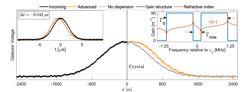
Figure 1: The spatial propagation of the pulse as it approaches the crystal. For clarity, the incoming and no dispersion pulses are scaled to the same intensity as the probe that propagates through the crystal. Unscaled data can be found in the supplement. The crystal is indicated by the vertical line. Here it can be seen that the advanced pulse peak comes out of the material before the incoming pulse peak enters. In the left inset the pulses are shown in time, with the advancement $\Delta t$. The $t_{\text{FWHM}}$ ratio between the advanced and reference pulse was 0.984. The pulse has a $t_{\text{FWHM}}$ of 5 μs. The right inset shows the gain structure used in the experiment and its effect on the refractive index. The gain structure width, $\Gamma_{\text{g}}$, and hole width $\Gamma_{\text{hole}}$ are indicated.

Manipulation of the group velocity, $v_{g}$, of pulses has been a subject of study for several decades. This manipulation is done by controlling the dispersion of the medium in which the pulse propagates. Controlling dispersion is vital in various applications, e.g. chirped pulse amplification Strickland and Mourou (1985) and in optical fibres Grüner-Nielsen et al. (2005). Reducing $v_{g}$ has led to an interesting field of research with a number of applications such as laser stabilisation Zhao et al. (2009); Horvath et al. (2022) and medical imaging A.Bengtsson et al. (2019). When working at the other end of the spectrum of $v_{g}$, in particular increasing $v_{g}$ beyond the vacuum light speed $c$, or when $v_{g}$ becomes negative, things become more abstract and less intuitive. One cannot violate causality, but negative group velocities can be achieved and can be described by the Kramers-Kronig relations Z.Fang et al. (2017). A number of experiments, starting as early as the 1960s, have been conducted to show that one can go into a regime where $v_{g}>c$ and can even go negative i.e. the pulse peak exits the material earlier than it entered Basov et al. (1966); S.Chu and S.Wong (1982); Segard and B.Macke (1985); R.Y.Chiao (1993); A.M.Steinberg et al. (1993); Rajan et al. (2015). The methods used include using the dispersion in an absorbing medium near a transparency Rajan et al. (2015) and non-linear amplification Basov et al. (1966). However, all these early experiments showed either a great deal of distortion of the pulses that were advanced in time Basov et al. (1966); S.Chu and S.Wong (1982) or the pulses were heavily attenuated Segard and B.Macke (1985); R.Y.Chiao (1993); A.M.Steinberg et al. (1993); Rajan et al. (2015). This left room for different interpretations of the result and the physical meaning of what was seen. In the strong attenuation case, for example, it was argued that the pulse was not advanced, but rather selectively attenuated such that the pulse peak appears to be shifted forward, but is still completely contained within the original pulse envelope.

To address the concerns raised regarding the physical interpretation, an undistorted, advanced pulse needed to be produced. It was suggested by Steinberg et al. Steinberg and Chiao (1994) that one could achieve undistorted pulse propagation through a transparent optical window between two gain regions. This was subsequently shown experimentally by Wang et al. L.J.Wang et al. (2000), using a Raman pumped system in a caesium vapour cell in $\Lambda$ configuration. However, the initial publication showed the advanced pulse still had some distortion. This among other factors made Ringenmacher and Mead Ringenmacher and Mead (2000) question the interpretation. To them, the 3$\%$ shape error with only 62 ns, 1.6$\%$, advancement on a pulse with $t_{\text{FWHM}}=$ 3.7 μs, and hence a time-bandwidth product of 0.007, seemed insufficient for a proper conclusion. Later Wang et al. published a second paper where they presented a pulse with similar advancement but without the previously observed distortion A.Dogariu et al. (2001).

In this work, we demonstrate almost an order of magnitude improvement in terms of time-bandwidth product, and relative pulse advancement. A Gaussian probe pulse with time full width half maximum (FWHM), $t_{\text{FWHM}}$ = 5 μs, was then used. This pulse was advanced by 0.543 μs which corresponds to 10.9$\%$ of the $t_{\text{FWHM}}$, see FIG 1. The relation of the FWHM of a Gaussian pulse in time and frequency is $t_{\text{FWHM}}=0.44/\nu_{\text{FWHM}}$, hence $\nu_{\text{FWHM}}$ = 88 kHz. This gives a time-bandwidth product, $|\Delta t|\cdot\nu_{\text{FWHM}}$, of 0.05, the corresponding group refractive index $n_{g}$ is hence -6.6$\cdot 10^{3}$. The shape was well maintained, the $t_{\text{FWHM}}$ stayed within 1.6$\%$ and the pulse power within 3.0$\%$ (upper bound estimation) of the reference.

We realised these results through the creation of two sharp, closely spaced gain regions in the inhomogeneous profile of a Europium-doped YSO crystal. This leads to a region of strong and linear anomalous dispersion between the gain regions, see FIG 1, left inset. The rare-earth (RE) system allows for much sharper gain features than were created in the caesium vapour cell L.J.Wang et al. (2000), and a group refractive index that is strongly negative. We are not aware of any previous result of a pulse time advancement with this large a time-bandwidth product, with as little distortion or attenuation.

Light pulses travel at the group velocity $v_{g}$ Saleh and Teich (2019):

$$v_{g}(\nu)=\frac{c}{n(\nu)+\nu\frac{dn(\nu)}{d\nu}}$$ (1)

With the speed of light in vacuum $c$, the refractive index $n(\nu)$ and the optical frequency $\nu$ Siegman (1986). From this expression, one can see that the refractive index and the change of it with frequency, or dispersion, influence the group velocity. In close vicinity of resonances, i.e. in absorption or gain regions, very strong dispersion can be achieved, see FIG 1. This behaviour can be described using the susceptibility, the imaginary and real parts of which govern the absorption and refractive index response respectively, using this, one can calculate the effect near such lines.

The real part of the susceptibility can be computed fairly simply by applying the parameters for the gain structures, $\Gamma_{g}$, and spacing of said peaks, or the hole width, $\Gamma_{\text{hole}}$, which are more than 14 MHz in frequency away from any absorbing structure. Equation 2 is then found for $n(\nu)$ in terms of $\alpha$, the absorption coefficient, and the parameters of the optical structure, see FIG 1 for clarification. The material parameters that allows for these assumptions are noted in the supplement. Since the region of interest is the transparent region around the centre frequency of the hole, a Taylor expansion is applied to get a linear approximation of $n(\nu)$:

$$n(\nu)=n_{\text{host}}+\frac{\alpha c}{\pi^{2}\nu_{c}}\left(\frac{1}{\Gamma_{\text{hole}}}-\frac{1}{\Gamma_{g}}\right)(\nu-\nu_{c})$$ (2)

With the background refractive index, $n_{\text{host}}$, and the central optical frequency, $\nu_{c}$. It should be noted that in the case of an inverted population the absorption coefficient, $\alpha$, will change sign and become a gain coefficient. A full derivation can be found in the supplement. By evaluating equation (2) at the centre frequency, the group refractive index $n_{g}=n(\nu)+\nu\frac{dn(\nu)}{d\nu}|_{\nu=\nu_{c}}$ is found. When the dispersion is large, $n_{\text{host}}$ is negligible and the dispersion term completely dominates the denominator, hence the group velocity $v_{g}(\nu=\nu_{c})$:

$$v_{g}=\frac{\pi^{2}}{\alpha}\left(\frac{1}{\Gamma_{\text{hole}}}-\frac{1}{\Gamma_{g}}\right)^{-1}$$ (3)

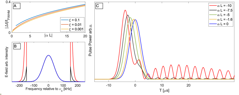
Figure 2: (a) Relative pulse advancement as a function of $\alpha L$ at fixed $\Gamma_{\text{hole}}$ (=300 kHz) for different degrees of tolerance in the pulse power increase. (b) Increase in pulse area of the electric field caused by the gain structure for different values of $\alpha L$ corresponding to those in (c). (c) Maxwell-Lindblad simulation of the propagation pulse with $t_{\text{FWHM}}$ = 5 μs and $\Gamma_{\text{hole}}$ = 300 kHz at various $\alpha L$, which shows the distortion caused by the amplified frequency regions in (b). The experimental conditions in FIG 1 correspond to $\alpha L=-1.6$

The resulting time advancement compared to propagation in vacuum is:

$$\Delta t=\frac{\alpha L}{\pi^{2}}\left(\frac{1}{\Gamma_{\text{hole}}}-\frac{1}{\Gamma_{g}}\right)$$ (4)

It is then evident that the stronger the gain and the narrower the spectral hole between the gain regions, the stronger the effect on the dispersion and thus the group velocity.

We will now briefly describe how the gain structure is prepared, with more details given in the supplementary material. The rare-earth ions are inhomogeneously broadened, such that different ions absorb at different frequencies. Further, the ions have three different degenerate ground hyperfine levels at zero magnetic field. Thus, it is possible to use optical pumping to spectrally tailor the absorption profile until the structure seen in the right inset of FIG 1 is created, except that the peaks have not yet been inverted and are therefore absorption peaks. In principle, ions far detuned from the absorption peaks also contribute to the refractive index, but as shown in the supplementary, the effect of these can be neglected. The laser used has a linewidth of a few kHz and the homogeneous broadening of the ions in the crystal is on the order of kHz, hence the created spectral structure is well described by step functions, as seen in FIG 1. The absorption peaks consist of different ion classes, where ion class refers to a unique optical transition for a given resonance frequency within the inhomogeneous profile. Since these transitions function as an effective two-level system for the inversion, they must be coherently excited using a single pulse. Furthermore, due to limited available laser power, the peaks must consist entirely of transitions with strong oscillator strength such that complete inversion can be achieved coherently well within the lifetime of the excited state. Said ions can be collected by targeting specific frequency ranges. The excited state lifetime in the Eu-system is 2 ms. However, in a long strongly inverted medium, amplified spontaneous emission (ASE) will reduce the upper state lifetime. Spontaneous emission events at the beginning of the inverted region will be amplified as they travel along the inverted region and stimulate emission from the upper state. This effect scales exponentially with the magnitude of the gain. Hence there is a maximal allowable $\alpha L_{max}$, which can be estimated considering that the spontaneous emission that occurs at the very first slice of the crystal will have the dominant effect in reducing the lifetime. The details are given in the supplement and the result is,

$$\alpha L_{max}=\ln\left(\frac{\gamma_{\text{rad,21}}}{W_{12}}\frac{z_{R}\lambda}{4n\pi L^{2}}\right)$$ (5)

With the radiative decay, $\gamma_{rad,21}$ on the ${}^{5}D_{0}\rightarrow~{}^{7}F_{0}$ transition used in the experiment, the Rayleigh length, $z_{R}$, crystal length, $L$, and the stimulated emission rate $W_{12}$. In our case $z_{R}\approx L$ was required to ensure full inversion, and from simulations it followed that halving the lifetime was acceptable as this would leave enough time for first the inversion pulse and then the propagation pulse. This in essence gives a fundamental limit for the maximal dispersion associated with the material. In Eu:YSO, this limit is $\alpha L_{max}\approx 18$. In our experiments, we were, however, limited by the available Rabi frequency and thus only inverted gain structures with an $\alpha L_{max}\approx 2$. Thus, with an improved experimental setup it is possible to improve the time-bandwidth product even more.

Let us now turn to the topic of distortion. To have a distortion free pulse the maximum bandwidth of a pulse, $\nu_{\text{FWHM}}$, is limited by the transmission window bandwidth, $\Gamma_{\text{hole}}$, and must remain below $\Gamma_{\text{hole}}$ by a factor that depends on the gain $\alpha L$. Pulses with large $t_{\text{FWHM}}$ achieve this but do not improve the relative advancement or time-bandwidth-product, which is the defining quantity one wants to maximise. A pulse with a Gaussian envelope in time, will also have a Gaussian envelope in in frequency, and hence has frequency content in the wings which extends into the inverted region. This means that part of the Gaussian pulse, however small, will get selectively amplified, which may distort the pulse. However, the Gaussian envelops falls off fast enough that beyond a certain bandwidth, the gain structures causes practically no distortion, i.e., there is a a level of tolerance when it comes to power leaking into the structure, before the pulse gets noticeably distorted, see FIG 2. This tolerance is connected to the magnitude of the gain of the structure, the frequency width of the optical window and the frequency width of the pulse. By multiplying the gain peaks with the $\vec{E}$-field of the Gaussian in frequency space and comparing the area under the pulse to that of the unperturbed pulse, one can get a quick and intuitive picture whether the distortion will be significant. The error depends on the magnitude of the gain and the product of the $t_{\text{FWHM}}$ and hole-width $\Gamma_{hole}$:

$$\xi=(1-e^{-\alpha L})\left(\operatorname{erf}\left(\frac{\pi t_{\text{FWHM}}\cdot\Gamma_{\text{hole}}}{4\sqrt{ln(2)}}\right)-1\right)$$ (6)

$\xi$ is then used as a measure of how much the pulse is amplified or distorted, with the error function, $\operatorname{erf}()$ . Consequently there is a gain versus bandwidth trade-off, the largest time-bandwidth product is achieved at the highest $\alpha L$, but this structure will require higher Rabi frequency of the inversion pulse and reduce the tolerance for power in the structure. This tolerance can be seen in FIG 2 (a), where the increase in distortion due to the local amplification of the pulses’, is plotted as a function of $\alpha L$ and the product of $\Gamma_{h}$ and $t_{\text{FWHM}}$. In time, this results initially in amplification and at larger values a ringing trailing the pulse front, which we both refer to as distortion for simplicity.

Our analysis shows that there is still some progress to be made by further optimising the experimental parameters of the system and that given enough laser power a relative pulse advancement of 30$\%$ or more could be possible depending on the allowed level of pulse distortion. Through this work, we have demonstrated that the rare earth system is an excellent test bed for applications which exploit strong dispersive properties.

Supplement

.1 Experimental setup

The experiments were conducted in a Y₂SiO₅ crystal with dimensions 14$\times$15$\times$21 mm doped to 1 at$\%$ natural abundance Europium containing both isotopes 151 and 153 in essentially equal proportion. The experiment was performed in a custom built closed cycle cryostat made by MyCryofirm in the temperature range 2-4 K.

The light pulses in this work were measured with a Hamamatsu S5973-02 photodiode and amplified by a femto - DHPCA-100 trans-impedance amplifier. Due to the low light power in the propagation pulses it was necessary to use high gain on the transimpedence amplifier. This limits the bandwidth of the detection to $f_{\text{BW}}=$ 1.8 MHz, hence we have a rise time, $t_{\text{rise}={0.35}/{f_{\text{BW}}}}$ of 0.2 $\mu s$. From simulations we know that this is sufficient bandwidth to detect any of the distortions that arise from clipping the structure, should they occur as can be seen in FIG 2 The optical setup is schematically shown in FIG 3, the light path is as follows, the shaped pulse come out of the PM fibre onto a beamsplitter that splits it into the reference path, where it is focused on an AOM that gates the propagation pulse from the inversion pulse and then finally on the detector. The rest of the light goes through the crystal, which we call the advanced path. For the advanced pulse it is first expanded, the polarisation is aligned with the crystal and filtered and then focused down into the crystal in the cryostat which is at 2 K after which it is collimated and then again gated by an AOM and then focused on the detector through a polariser and filter that remove the fluorescence of the crystal and otherwise scattered light. Significant care was put into adjusting the AOM delay such that pulses arrived at the detectors at the same time when no structure was prepared.

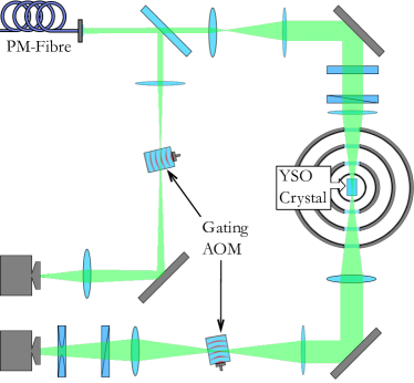
Figure 3: Optical setup during the experiment.

.2 Preparation of structure

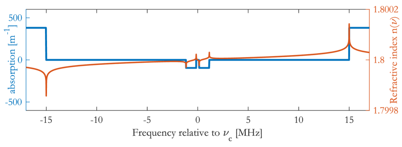
Figure 4: Simulated Dispersion effect of the gain structure and optical window

Experiments were performed on the ${}^{7}F_{0}\rightarrow$ ${}^{5}D_{0}$ transition. A six level simulator was used to keep track of the ions and determine the optimal frequencies for the optical pumping and creating the absorption and transmission structures, such that the ions that make up the structure have their strong transition at these frequencies. The ion classes with the weak transition in these frequency range are not targeted for the burn back. A 29 MHz wide transmission widow was first created using optical pumping. Two absorbing structures each 1 MHz wide, centred at $\pm$ 650 kHz from the centre of the optical transmission window, leaving a 300 kHz transmission window at the centre frequency were created see FIG 4. The collected ions correspond to the transitions $\ket{1/2g}\rightarrow\ket{5/2e}$, $\ket{3/2g}\rightarrow\ket{3/2e}$ and $\ket{5/2g}\rightarrow\ket{1/2e}$, which have the strong oscillator strengths and hence will be easier to invert. If the ions with low oscillator strength would not be removed, these ions would take up part of the energy from the inversion pulse, but would not reach inversion. This means that there will be an absorbing component in the structure leading to the effective gain to be much lower and as such the advancement would be reduced. The population inversion was then simulated using a Maxwell-Lindblad simulator, which used a simplified two level system where the oscillator strength has been averaged corresponding to the fraction of the respective ions collected and estimated available laser power. The two peaks are inverted using a ”sech-scan pulse”, a frequency scan spliced in the middle of a sechhyp pulse Park and Garwood (2009). A Gaussian pulse, $t_{\text{FWHM}}$ = 5 μs, was used as the propagation pulse. From the Maxwell-Lindblad simulations the parameters for the experiment were determined, as well as the type of distortion, should the pulse power in the gain structures exceed the distortion free limit. This can be seen in FIG 2, where various magnitudes of $\alpha L$ are shown.

.3 Distortion

To get a quick and intuitive idea of what will happen to the pulse for certain $t_{\text{FWHM}}$ and $\Gamma_{\text{hole}}$ with a given $\alpha L$ one can look at the increase of pulse area in frequency space. This will give a clear representation of which frequency content is amplified and how large it is compared to the original envelope, see FIG 2. To find a badness number, we start with a Gaussian pulse in time,

$$E(t)=exp\left({-\frac{4ln(2)t^{2}}{t_{\text{FWHM}}^{2}}}\right)$$ (7)

Which naturally remains Gaussian in frequency,

$$E(\nu)=\frac{t_{\text{FWHM}}\sqrt{\pi}}{2\sqrt{ln(2)}}exp\left({-\frac{t_{\text{FWHM}}^{2}\pi^{2}\nu^{2}}{4ln(2)}}\right)$$ (8)

One can then write the expression for the gain structure as a function of frequency $\gamma(\nu)$. Since a Gaussian quickly drops off in amplitude, the effect of the gain structure will mostly come from the frequencies closest the pulse centre frequency, and the frequency content far in the wings will have little influence on the distortion. Thus the product of the amplification and the power in the wing of the pulse will be negligible already by before the end of the proposed frequency width. This allows us to simplify the gain structure to be infinitely broad but with the transmission window around the centre frequency. Hence $\gamma(\nu)$:

$$\gamma(\nu)=exp\left(-\alpha L\left(\theta\left(-\frac{\Gamma_{h}}{2}+\nu\right)+\theta\left(-\frac{\Gamma_{h}}{2}-\nu\right)\right)\right)$$ (9)

Simply multiplying these and then integrating the product gives a measure of the energy in the pulse, then subtracting the original power leads to the error:

$$\xi={\int_{-\infty}^{\infty}E(\nu)\gamma(\nu)d\nu}-{\int_{-\infty}^{\infty}E(\nu)d\nu}$$ (10)

Solving this lead to:

$$\xi=(1-e^{-\alpha L})\left(\operatorname{erf}\left(\frac{\pi t_{\text{FWHM}}\cdot\Gamma_{\text{hole}}}{4\sqrt{ln(2)}}\right)-1\right)$$

The effect on the dispersion, taking in account the edges of the 29 MHz wide optical window is shown in FIG 4. It is seen that although there is positive dispersion outside the gain structure, the dispersion within the transmission window is still negative. Furthermore it is clearly seen that the strongest dispersion effects occur closest to the spectral features.

.4 Derivation of $n(\nu)$

The refractive index for the transmission windwo and the material combined is:

$$n(\nu)=n_{\text{host}}+\frac{\chi_{real}}{2n_{\text{host}}}$$ (11)

Start from the susceptibility:

$$\chi_{h}(\nu)=-\frac{2j\alpha_{0}cn_{\text{host}}}{\nu_{\text{central}}\pi^{2}(\Gamma_{h}+2j(\nu-\nu_{0}))}$$ (12)

Assume that the absorption profile looks flat from the perspective of the pit/structure and that there is no background absorption in the pit:

$$g(\nu)=\theta\left(-\frac{\Gamma_{\text{hole}}}{2}+\nu_{0}\right)+\theta\left(-\frac{\Gamma_{\text{hole}}}{2}-\nu_{0}\right)\\ -\theta\left(-{\Gamma_{g}}-\nu_{0}\right)-\theta\left(-\Gamma_{g}+\nu_{0}\right)$$ (13)

Here $\theta(\nu)$ represents the Heaviside step-function. The real part of $\chi_{h}(\nu)$ describes the refractive index, the imaginary part the absorption. Then to get the $\Re(\chi_{h}(\nu))$ for the structure the integral of the susceptibility multiplied with the absorption profile must be computed:

$$\chi_{real}=\int^{\infty}_{\infty}g(\nu)\Re(\chi_{h}(\nu))d\nu_{0}$$ (14)

Furthermore assume that the structure terminates at $\Gamma_{g}$ and that beyond this point the absorption is far enough away to not have a significant influence. One could consider these effects by by simply adding similar terms with the appropriate boundary conditions, but as can be seen from FIG 4 it has little effect on the result. The simplified situation is described by:

$$\chi_{real}=\int^{-{\Gamma_{\text{hole}}}/{2}}_{-\Gamma_{g}}\Re(\chi_{h}(\nu))d\nu_{0}+\int^{\Gamma_{g}}_{{\Gamma_{\text{hole}}}/{2}}\Re(\chi_{h}(\nu))d\nu_{0}$$ (15)

Then computing this integral this gives:

$$\begin{split}\chi_{real}=-\frac{\alpha_{0}cn_{\text{host}}}{2\pi^{2}\nu_{\text{central}}}\\ ln\left(\frac{4\Gamma_{g}^{2}+8\Gamma_{g}\nu+4\nu^{2}+\Gamma_{h}^{2}}{4\nu^{2}+4\Gamma_{\text{hole}}\nu+\Gamma_{h}^{2}+\Gamma_{\text{hole}}^{2}}\right)\\ +ln\left(\frac{4\nu^{2}-4\Gamma_{\text{hole}}\nu+\Gamma_{h}^{2}+\Gamma_{\text{hole}}^{2}}{4\Gamma_{g}^{2}-8\Gamma_{g}\nu+4\nu^{2}+\Gamma_{h}^{2}}\right)\end{split}$$ (16)

The homogeneous linewidth $\Gamma_{h}$ will be negligible compared to the other frequency widths so can be ignored giving:

$$\begin{split}\chi_{real}=-\frac{\alpha_{0}cn_{\text{host}}}{2\pi^{2}\nu_{\text{central}}}\times\\ ln\left(\left(\frac{4\Gamma_{g}^{2}+8\Gamma_{g}\nu+4\nu^{2}}{4\nu^{2}+4\Gamma_{\text{hole}}\nu+\Gamma_{\text{hole}}^{2}}\right)\left(\frac{4\nu^{2}-4\Gamma_{\text{hole}}\nu+\Gamma_{\text{hole}}^{2}}{4\Gamma_{g}^{2}-8\Gamma_{g}\nu+4\nu^{2}}\right)\right)\end{split}$$ (17)

using 11 and applying a Taylor expansion in $\nu$ around the centre of the pit:

$$n(\nu)=n_{\text{host}}+\frac{\alpha_{0}c}{\pi^{2}\nu_{\text{central}}}\left(\frac{1}{\Gamma_{g}}-\frac{2}{\Gamma_{\text{hole}}}\right)\nu$$ (18)

.5 Unscaled pulses and reference

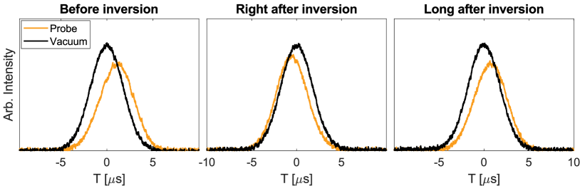
Figure 5: Probe pulse sequence, raw data, where vacuum refers to the pulse that does not travel through the crystal but is picked off by the beamsplitter as shown in FIG 3

In FIG 5 the pulse sequence from the experiment is shown. After the structure is prepared, we sent in an initial pulse without inversion, to probe the collected $\alpha L$ without disturbing the structure. Between probe pulses a 15 ms wait was added to allow proper relaxation. After which an inversion pulse is sent immediately followed by a probe pulse. Finally after another 15 ms wait, a third probe pulse is sent to asses the structure after absorption. This data is not scaled, but as one can see from the delayed pulse compared to the advanced pulse there is minimal amplification of the advanced pulse. In the main paper the reference pulses are scaled down to the probe pulses to more clearly display the effect. The vacuum pulse has higher intensity than the probe pulses.

.6 Maximal gain

We assumed excited volume of the crystal to be roughly cylindrical. Then a spectral packet that originated at the very start of the crystal will reach the end with intensity:

$$I_{ij}\approx\frac{\gamma_{\text{rad,ij}}h\nu r^{2}}{4\sigma_{ij}L^{2}}e^{-\alpha_{ij}L}$$ (19)

p552 Siegman (1986), where the subscripts indicate the specific levels involved. We have $\gamma_{\text{rad,tot}}=\frac{1}{2~{}\unit{ms}}=500~{}\unit{Hz}$ the radiative decay for the respective real atomic transitions, $r$ the radius of the cylinder, the absorption on a particular transition, $\alpha_{ij}$, note that $\alpha_{ij}<0$ when the population is inverted. Then using the relation of the stimulated transition rate and intensity one can find the relationship between the radiative decay rate and the transition rate. The stimulated emission rate $W_{ij}$ between a level $i$ and $j$ is given by:

$$W_{ij}=\frac{\sigma_{ij}I_{ij}}{h\nu}$$ (20)

combining these two equations leads to the ratio of the stimulated and radiative rates,

$$\frac{W_{ij}}{\gamma_{\text{rad}}ij}\approx\left(\frac{r}{2L}\right)^{2}e^{-\alpha_{ij}L}$$ (21)

p522 Siegman (1986), with beam radius, $r$ and the crystal length, $L$ . The ${}^{5}D_{0}\rightarrow~{}^{7}F_{0}$, transition is used for this experiment, but there is also relaxation to the other ${}^{7}F_{J}$ levels, hence it is important to know what dominates the stimulated emission.

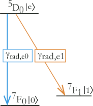
Figure 6: Relevant levels for radiative decay. The ${}^{5}D_{0}$ is denoted by $\ket{e}$, the ${}^{7}F_{0}$ by $\ket{0}$ and the ${}^{7}F_{1}$ by $\ket{1}$

The branching ratio for the ${}^{5}D_{0}\rightarrow~{}^{7}F_{0}$, $\gamma_{\text{rad, ceo}}$ can be calculated from the oscillator strength:

$$\gamma_{rad,e0}=F_{e0}3^{*}\gamma_{\text{rad, ceo}}$$ (22)

Siegman (1986); Könz et al. (2003) For this transition $F_{e0}=1.3\cdot 10^{-8}$, and, with the light polarisation aligned with the D1 axis,

$$3^{*}_{e0}=\frac{3.9}{\sqrt{3.9^{2}+0.8^{2}}}\cdot 3=2.94$$ (23)

the classical electron oscillator radiative decay rate, $\gamma_{rad,ceo}$ is given by,

$$\gamma_{rad,ceo}=2.47\cdot 10^{-22}~{}nf_{a}^{2}$$ (24)

with the optical frequency, $f_{a}$, and the index of refraction, n, hence $\gamma_{\text{rad,e0}}=4.23$. Now $\gamma_{\text{rad, e0}}/\gamma_{\text{rad, tot}}=$ 0.8$\%$, which means that 99.2$\%$ from the ${}^{5}D_{0}$ relaxes through the ${}^{7}F_{J\in 1,2,3,4,5,6}$ lines. However all the ${}^{7}F_{J\in 2,3,4,5,6}$ are quite broad, the exception is ${}^{7}F_{1}$. Which is the narrowest and strongest and will dominate those dynamics. Könz et al. report it to be much narrower than 6 GHz Könz et al. (2003), and the structure that we invert is about 2.3 MHz wide. So as long as the ${}^{7}F_{1}$ is wide compared to this, it can be ignored. One then needs to compute the cross sections of the transitions, $\sigma_{ij}$

$$\sigma_{ij}(\nu)=\frac{3^{*}\gamma_{rad,ij}}{\Delta\nu_{\text{Lorentz}}}\left(\frac{\lambda}{n}\right)^{2}$$ (25)

In term the absorption depends on the cross section,

$$\alpha_{ij}=\Delta N_{ij}\sigma_{ij}$$ (26)

If we assume that the linewidth for the ${}^{3}D_{0}\rightarrow~{}^{7}F_{1}$ is on the order of 1 Ghz, and we take $\sigma_{e0}=1.2\cdot 10^{-18}$ m^2 from Kriváchy et al. Kriváchy et al. (2023). The radiative decay rate for ${}^{5}D_{0}\rightarrow~{}^{7}F_{1}$ was estimated to be $\gamma_{\text{rad, e1}}\approx 40$ from the relative line strengths in FIG 1b in Yano et al. (1991), due to the limited resolution this was a rather crude estimate. Then for the $e1$ transition one gets

$$\Delta\nu_{\text{Lorentz}}=\frac{3}{\sigma_{\text{{e1}}}}\left(\frac{\lambda_{\text{e1}}}{n}\right)^{2}\gamma_{\text{rad},e1}$$ (27)

Thus $\sigma_{\text{e1}}=1.28\cdot 10^{-20}$ m^2. Which means the stimulated ASE decay is completely dominated by the ${}^{5}D_{0}\rightarrow~{}^{7}F_{0}$. So we can simply take

$$\frac{W_{e0}}{\gamma_{\text{rad,e0}}}\approx\left(\frac{\sqrt{\frac{z_{R}\lambda}{n\pi}}}{2L}\right)^{2}\cdot e^{-\alpha_{e0}L}$$ (28)

Where $z_{R}$ is the Raleigh range $\lambda$ the wavelength, $W_{e0}$ the stimulated emission rate. Hence, given an acceptable reduction of the lifetime, given by the ratio $W_{e0}/\gamma_{\text{rad,e0}}$, one can determine the maximum $\alpha L_{max}$:

$$\alpha L_{max}=\ln\left(\frac{\gamma_{\text{rad,e0}}}{W_{e0}}\frac{z_{R}\lambda}{4n\pi L^{2}}\right)$$ (29)

This gives $\alpha L_{max}=17.3$ in our case.

References

- Strickland and Mourou (1985) D. Strickland and G. Mourou, Optics Communications 55, 447 (1985).
- Grüner-Nielsen et al. (2005) L. Grüner-Nielsen, M. Wandel, P. Kristensen, C. Jørgensen, L. V. Jørgensen, B. Evold, B. Pálsdóttir, and D. Jakobsen, Journal of lightwave technology 23, 3566 (2005).
- Zhao et al. (2009) Y. Zhao, H.-W. Zhao, X.-Y. Zhang, B. Yuan, and S. Zhang, Optics & Laser Technology 41, 517 (2009).
- Horvath et al. (2022) S. Horvath, C. Shi, D. Gustavsson, A. Walther, A. Kinos, S. Kröll, and L. Rippe, New Journal of Physics 24, 1 (2022).
- A.Bengtsson et al. (2019) A.Bengtsson, D.Hill, M.Li, M.Di, M.Cinthio, T.Erlöv, S.Andersson-Engels, N.Reistad, A.Walter, L.Rippe, and S.Kröll, Biomedial Optics Express 10, 5565 (2019).
- Z.Fang et al. (2017) Z.Fang, H. Cai, G. chen, and R. Qu, “Single frequency semiconductor lasers,” in Single Frequency Semiconductor Lasers, Vol. 9, edited by A. Majumdar, A. Bjarklev, H. Caulfield, G. Marowsky, M. W. Sigrist, C. Someda, and M. Nakazawa (Springer, Singapore, 2017) pp. 168–169.
- Basov et al. (1966) N. Basov, R. Ambartsumyan, V. Zuev, P. Kryukov, and V. Letokhov, Soviet Physics JETP 23 (1966).
- S.Chu and S.Wong (1982) S.Chu and S.Wong, Physical Review letters 48, 738 (1982).
- Segard and B.Macke (1985) B. Segard and B.Macke, Physics Letters 109A, 213 (1985).
- R.Y.Chiao (1993) R.Y.Chiao, Phys. Rev. A 48 (1993).
- A.M.Steinberg et al. (1993) A.M.Steinberg, P.G.Kwiat, and R.Y.Chiao, Phys. Rev. Lett. 71 (1993).
- Rajan et al. (2015) R. P. Rajan, A. Redbane, and H. Riesen, Journal of the optical society of america B 32 (2015).
- Steinberg and Chiao (1994) A. M. Steinberg and R. Y. Chiao, Physical Review A 49, 2071 (1994).
- L.J.Wang et al. (2000) L.J.Wang, A.Kuzmich, and A.Dogariu, Nature 406, 277 (2000).
- Ringenmacher and Mead (2000) H. I. Ringenmacher and L. R. Mead, “Comment on ”Gain-Assisted Superluminal light Propagation”,” (2000).
- A.Dogariu et al. (2001) A.Dogariu, A.Kuzmich, and L.J.Wang, Phys. Rev. A 63 (2001).
- Saleh and Teich (2019) B. Saleh and M. Teich, Fundamentals of Photonics (Wiley, 2019).
- Siegman (1986) A. E. Siegman, Lasers, 1st ed. (University Science Books, Mill Valley, CA, 1986).
- Park and Garwood (2009) J.-Y. Park and M. Garwood, Magn Reson Med. 61, 175 (2009).
- Könz et al. (2003) F. Könz, Y. Sun, C. Thiel, R. Cone, R. Equall, R. L. Hutcheson, and R. Macfarlane, Physical Review B 68, 1 (2003).
- Kriváchy et al. (2023) T. Kriváchy, K. T. Kaczmarek, M. Afzelius, J. Etesse, and G. Haack, Physical Review A 107 (2023).
- Yano et al. (1991) R. Yano, M. Mitsunaga, and N. Uesugi, Optics Letters 16 (1991).