A probabilistic model of relapse in drug addiction

Abstract

More than 60$\%$ of individuals recovering from substance use disorder relapse within one year. Some will resume drug consumption even after decades of abstinence. The cognitive and psychological mechanisms that lead to relapse are not completely understood, but stressful life experiences and external stimuli that are associated with past drug-taking are known to play a primary role. Stressors and cues elicit memories of drug-induced euphoria and the expectation of relief from current anxiety, igniting an intense craving to use again; positive experiences and supportive environments may mitigate relapse. We present a mathematical model of relapse in drug addiction that draws on known psychiatric concepts such as the “positive activation; negative activation” paradigm and the “peak-end” rule to construct a relapse rate that depends on external factors (intensity and timing of life events) and individual traits (mental responses to these events). We analyze which combinations and ordering of stressors, cues, and positive events lead to the largest relapse probability and propose interventions to minimize the likelihood of relapse. We find that the best protective factor is exposure to a mild, yet continuous, source of contentment, rather than large, episodic jolts of happiness.

[1]organization=Department of Computational Medicine, addressline=UCLA, city=Los Angeles, postcode=90095-1766, state=CA, country=USA

[2]organization=Department of Computational Medicine, addressline=UCLA, city=Los Angeles, postcode=90095-1766, state=CA, country=USA

[3]organization=Department of Mathematics, addressline=California State University at Northridge, city=Los Angeles, postcode=91330, state=CA, country=USA

1 Introduction

Illicit drug abuse remains a major problem in the United States. Despite decades of research and the implementation of policies ranging from harm reduction to punitive measures, drug overdose deaths have increased dramatically over the past 40 years, surpassing 107,000 fatalities in 2022 [1]. According to the 2021 National Survey on Drug Use and Health (NSDUH) about 3.3$\%$ of the population aged 12 and above misused opioids in 2021, the latest year for which data is available [2].

Our understanding of substance abuse has also evolved in the past 40 years: addiction, once viewed as a lifestyle choice, is now considered a chronic brain disease characterized by the compulsive seeking and using of drugs despite harmful consequences. Drugs change the neurocircuitry of the brain reward system leading to distortions in how non-drug rewards are processed, diminished self-control, increased sensitivity to stressful events, and the prioritization of drug consumption above all. Over time, tolerance emerges so that for pleasurable sensations to persist or for withdrawal symptoms to dampen, one must increase dosage or intake frequency. Since drug-induced damage to the brain is long-lasting and structural, treatment is a complex process, spanning several years and necessitating behavioral and pharmacological approaches [3]. While detoxification requires a few weeks, remaining sober over a lifetime is challenging: according to the National Institute of Drug Abuse (NIDA) more than 60$\%$ of those with substance use disorder relapse within one year [4, 5, 6]. The likelihood of relapse is highest in the first months after detoxification [7]; however, relapse is possible even after many years of abstinence [8]. Since those in recovery may have lost their previously built tolerance, de-novo consumption, even in smaller amounts than during active use, may cause overdoses.

Given the severity of the problem, it is important to understand the psychological, behavioral and environmental factors that characterize drug use [9, 10, 11]. Many studies have been developed over the years to illustrate the process of addiction, utilizing psychiatric concepts, brain imaging studies, and behavioral surveys [12, 13, 14, 15, 16, 17, 18, 19]. Forecasting tools and data analyses have also been presented [20, 21, 22]. There is however no explicit quantitative framework to describe the cognitive processes behind relapsing, although the presence of emotional stressors and sensory cues are known to be major influences [23, 24, 25, 26, 27, 28].

Among the most vivid memories of addicts (and former addicts) is the pleasure associated with the first time drugs were consumed, often the most euphoric part of the drug-taking experience. “Chasing the first high” is a common refrain, regardless of how far in the past the first high occurred. This aligns with the so-called “peak-end” rule according to which the memory of a past experience is biased by its most emotionally intense period (the high in this case), and its ending [29]. Other less intense periods, or even the entire duration of the experience, do not carry as much mnemonic weight [30]. Relapses may be triggered by stressful events that lead to the retrieval of euphoric drug-related memories, such as the first high, and to the anticipation of future euphoria if drugs are consumed again [31]. Drugs are viewed as a way to alleviate the negative affects induced by current stressors and to increase short term wellbeing [32]. External cues such as persons, objects, locations, situations connected to past drug use may also evoke memories associated with prior drug consumption and pleasure [33, 34]. When stressors and/or cues are present, the associations between drug use and pleasure (or mitigation of pain) may lead to intense cravings and relapse [35]. The goal of this work is to create a mathematical framework whereby the relapse likelihood is described as a function of quantities that represent life stressors occurring at various times and with varying intensity, cues and memories related to the previous drug addiction experience, and changes to the neurocircuitry of the former user.

In the next section, we introduce our mathematical model in which the relapse rate is framed in terms of the mental state of the user, drug availability and the presence of cues. Known psychological and behavioral processes associated with addiction, such as reward collection, tolerance, adaptation, and decision-making [36, 17, 18, 19, 37, 38] are integrated into a probabilistic model of relapse events. Most critical of these components is a “mental state” that is driven by positive life experiences, stressors and cues. Predictions of our model, subject to different sequences of positive events, stressors, and cues are shown in Section 3. We end with further discussion and conclusions in Section 4.

2 Dynamical systems model for relapse

2.1 Relapse rates and probabilities

We begin by assuming that drug consumption has ceased and that the individual started recovery at time $t=0$. At any time $t>0$ of the recovery phase, the probability per unit time of relapse, defined as the instant the individual breaks sobriety by drug intake, is assumed to be driven by the user’s mental state $M(t)$, which can be either positive or negative, the influence $C(t)$ of any external cues that remind the user of past drug taking euphoria, and the current availability of drugs, $I(t)$. Positive values of the mental state $M(t)$ indicate well-being and optimism, and negative values represent discontent and malaise. Drug availability can be described by a continuous variable that represents the ease with which drugs are acquired and consumed. For simplicity, we binarize $I(t)$ so that $I(t)=1$ indicates that drugs are readily available and $I(t)=0$ that they cannot be procured. Finally, cues are assumed to amplify the relapse rate via a non-negative motivation term $C(t)\geq 0$. Together, we let $M(t)$, $C(t)$ and $I(t)$ shape the rate of relapse $R(t)$ via

$$R(t)=I(t)R_{0}e^{C(t)}e^{-M(t)}.$$ (1)

In this model, $R(t)\mathrm{d}t$ can be interpreted as the probability that the relapse event (first use of drugs after $t=0$) occurred between $t$ and $t+\mathrm{d}t$. Even though the instantaneous relapse rate does not explicitly depend on history or memory, it depends on $C(t)$ and $M(t)$ which dynamically evolve, implicitly imparting event histories into the current relapse rate. Eq. 1 indicates that if the drug supply is unrestricted ($I(t)=1$), no cues are present ($C(t)=0$), and an individual is under a “neutral” mental state ($M(t)=0$) the rate of relapse is given by a reference baseline $R(t)=R_{0}$. Negative values of the mental state $M(t)<0$ increase the relapse rate, conversely $R(t)$ vanishes in the case of a strongly positive mental state $M(t)\gg 1$. An alternative model for $R(t)$ may include a maximal saturated value $R_{\rm max}$, representing the fastest possible rate of acquiring and consuming drugs and that is attained when $C(t)-M(t)$ surpasses a positive threshold. Finally, the probability of relapsing by time $T$, $P(T)$, can be written in terms of the survival (against relapse) probability up to time $T$, $S(T)$ given by

$$S(T)=\displaystyle e^{-\int_{0}^{T}R(t){\rm d}t},\quad P(T)=1-S(T).$$ (2)

Next, we describe an event-based model for the dynamics of the mental state $M(t)$.

2.2 The PA/NA mental state model

The so-called “Positive Activation, Negative Activation” (PA/NA) model posits that affects arising from positive and negative experiences are not coupled [39, 40, 41] and might be processed on different neural substrates [42, 43]. Thus a realistic representation of the mental state $M(t)$ is as a sum of two contributions, $M(t)=M_{\rm a}(t)+M_{\rm b}(t)$, where positive events affect $M_{\rm a}(t)$, negative ones affect $M_{\rm b}(t)$, and the two evolve independently. Negative events, or stressors, are known to impact one’s mental state more than positive ones, a neurological phenomenon known as the “negativity bias” [44]; recent studies also show that stressors tend to affect drug users more than the general population [45, 46], and that drug abuse produces hypersensitivity to negative emotional distress [25, 47, 48]. Note that the exponential term $e^{-M(t)}$ in Eq. 1 weights negative mental states more than positive ones, in accordance with negativity bias [44]. We model the dynamics of $M_{\rm a}$ and $M_{\rm b}$ using different processing rates $\kappa_{\rm a}(t)$ and $\kappa_{\rm b}(t)$ as

$$\frac{\mathrm{d}M_{\rm a}}{\mathrm{d}t}= -\kappa_{\rm a}(t)M_{\rm a}+\!\sum_{i,t\geq t_{i}^{\rm a}}\!A_{i}\delta(t-t_{i}^{\rm a}),$$ (3a)

$$\frac{\mathrm{d}M_{\rm b}}{\mathrm{d}t}= -\kappa_{\rm b}(t)M_{\rm b}-\!\sum_{j,t\geq t_{j}^{\rm b}}\!B_{j}\delta(t-t_{j}^{\rm b}).$$ (3b)

In Eq. 3a $A_{i}>0$ is the intensity of positive life event $i$, as experienced by the individual in recovery, occurring at time $t_{i}^{\rm a}$ and $\kappa_{\rm a}(t)>0$ is the processing rate that returns $M_{\rm a}(t)$ to steady state. Similarly for $-B_{j}<0$, $t_{j}^{\rm b}$ and $\kappa_{\rm b}(t)$ in Eq. 3b. Since $M_{\rm a}$ and $M_{\rm b}$ are decoupled and $\kappa_{\rm a}(t)\neq\kappa_{\rm b}(t)$, Eqs. 3a and 3b are our mathematical representation of the PA/NA model. We solve them assuming that there are no initial affects, $M_{\rm a}(t=0)=M_{\rm b}(t=0)=0$ and that $\kappa_{\rm a}(t)=\kappa_{\rm a}$ and $\kappa_{\rm b}(t)=\kappa_{\rm b}$ are time-independent. Non-zero initial affects can be incorporated by setting $A_{1}=M_{\rm a}(t=0)$ at $t_{i=1}^{\rm a}=0$ or $B_{1}=-M_{\rm b}(t=0)$ at $t_{j=1}^{\rm b}=0$ in the sequence of positive or negative life events. Time-dependent $\kappa_{\rm a}(t),\kappa_{\rm b}(t)$ are discussed in the Appendix. We solve Eqs. 3a and 3b under the above approximations to find

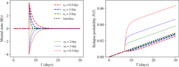
Figure 1: Mental state at time $t$, $M(t)$, and the probability of relapse before time $T$, $P(T)$, upon exposure to a single stressor $\{-B_{1},t_{1}^{\rm b}\}$ or to a single positive event $\{A_{1},t_{1}^{\rm a}\}$ for three processing rates $\kappa_{\rm b}\text{ or }\kappa_{\rm a}=2,1,0.5$/day with $B_{1}=A_{1}=4$, $t^{\rm b}_{1},t^{\rm a}_{1}=7$ days, $R_{0}=10^{-3}$/day ,$~{}M_{0}=0$. The relapse probability decreases with $\kappa_{\rm b}$ so that the longer a stressor impacts one’s mental state, the larger the likelihood of relapse. The opposite is true for positive events, for which the longer memory of a positive event is retained, the less likely relapse is. Note the more pronounced effect of the negative mental state $B_{1}$, compared to the positive one $A_{1}$ under the same processing rate despite their amplitudes being the same. The mental state $M(t)=M_{\rm a}(t)+M_{\rm b}(t)$ is given by Eqs. 4; the relapse probability $P(T)$ by Eqs. 1 and 2.

$$M_{\rm a}(t)= \!\sum_{i,t\geq t_{i}^{\rm a}}\!A_{i}e^{-\kappa_{\rm a}(t-t_{i}^{\rm a})},$$ (4)

$$M_{\rm b}(t)= -\!\sum_{j,t\geq t_{j}^{\rm b}}\!B_{j}e^{-\kappa_{\rm b}(t-t_{j}^{\rm b})}.$$

The mental state integrated up to time $T$ after $n_{\rm a}$ positive and $n_{\rm b}$ negative life events, such that $t_{n_{\rm a}}^{\rm a}\leq T\leq t_{n_{\rm a}+1}^{\rm a}$ and $t_{n_{\rm b}}^{\rm b}\leq T\leq t_{n_{\rm b}+1}^{\rm b}$, is thus given by

$$\int_{0}^{T}\!M(t)\mathrm{d}t= \int_{0}^{T}\!\big{(}M_{\rm a}(t)+M_{\rm b}(t)\big{)}\mathrm{d}t$$ (5)

$$\>= \frac{1}{\kappa_{\rm a}}\sum_{i=1}^{n_{\rm a}}\!A_{i}\left(1-e^{-\kappa_{\rm a}(T-t_{i}^{\rm a})}\right)-\frac{1}{\kappa_{\rm b}}\sum_{j=0}^{n_{\rm b}}\!B_{j}\left(1-e^{-\kappa_{\rm b}(T-t_{j}^{\rm b})}\right).$$

The effects of a sequence of $n_{\rm a}$ events defined by $\{A_{i},t_{i}^{\rm a}\}$ on the integrated mental state in Eq. 5 can be reproduced by a single event of amplitude $Z_{\rm a}$ at specific time $t_{\rm a}$

$$Z_{\rm a}=\sum_{i=1}^{n_{\rm a}}A_{i},\,\,\,t_{\rm a}=\frac{1}{\kappa_{\rm a}}\ln\left[\displaystyle{\frac{\sum_{i=1}^{n_{\rm a}}A_{i}e^{\kappa_{\rm a}t_{i}^{\rm a}}}{\sum_{i=1}^{n_{\rm a}}A_{i}}}\right].$$ (6)

Similarly, a sequence of $n_{\rm b}$ events $\{-B_{j},t_{j}^{\rm b}\}$ generates an integrated mood that can be reproduced by single event

$$Z_{\rm b}=\sum_{j=1}^{n_{\rm b}}B_{j},\,\,\,t_{\rm b}=\frac{1}{\kappa_{\rm b}}\ln\left[\displaystyle{\frac{\sum_{j=0}^{n_{\rm b}}B_{j}e^{\kappa_{\rm b}t_{j}^{\rm b}}}{\sum_{i=0}^{n_{\rm b}}B_{j}}}\right].$$ (7)

Thus far, we have modeled the dynamics of positive and negative mental state variables. Included in the relapse rate $R(t)$ is also a dependence on random cues that trigger the memory of drug-induced euphoria. The model for cues shares many features of the negative mood variable and is described below.

2.3 External cues

Here we discuss representations for $C(t)\geq 0$. External cues can trigger memories of the pleasurable feelings associated with drug taking [49, 50]. We model these memories as impulses occurring at times $t_{\ell}^{\rm c}$ whose effects decay with rate $\kappa_{\rm c}$. Thus, the dynamics of $C(t)$, the overall motivation from cues, is given by

$$\frac{\mathrm{d}C}{\mathrm{d}t}=-\kappa_{\rm c}(t)C+\!\sum_{\ell,t\geq t_{\ell}^{\rm c}}\!C_{\ell}\delta(t-t_{\ell}^{\rm c}).$$ (8)

The amplitude $C_{\ell}$ represents the mnemonic strength of a given cue. By the peak-end rule, we assume that the most intense memory is proportional to $w_{\rm peak}>0$, the largest reward response during addiction, and set $C_{\ell}=w_{\rm peak}$ for all $\ell$. We also assume the decay rate $\kappa_{\rm c}(t)$ associated with the permanence of the cue in one’s memory is a constant, $\kappa_{\rm c}(t)=\kappa_{\rm c}$ and that there are no initial cues, $C(t=0)=0$, which leads to

$$C(t)=w_{\rm peak}\sum_{\ell,t\geq t_{\ell}^{\rm c}}e^{-\kappa_{\rm c}(t-t^{\rm c}_{\ell})}.$$ (9)

3 Results

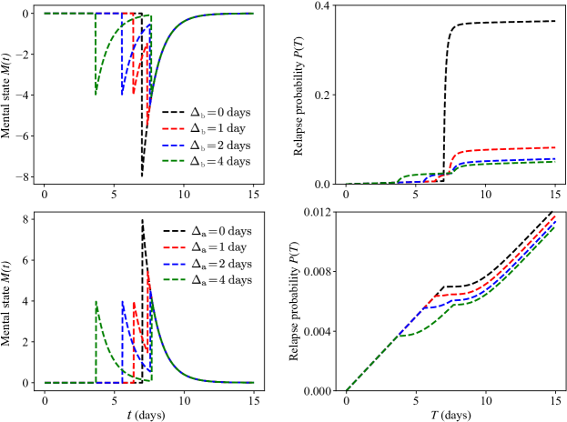
Figure 2: Top row: Mental state $M(t)$ and relapse probability $P(T)$ upon exposure to two stressors $\{-B_{1},t_{1}^{\rm b}\}$ and $\{-B_{2},t_{2}^{\rm b}\}$ separated by lag times $\Delta_{\rm b}=t_{2}^{\rm b}-t_{1}^{\rm b}=0,1,2,4$ days and obtained using Eqs. 1, 2, 4, and 12. Parameters are $\kappa_{\rm b}=1$/day, $B_{1}=B_{2}=4$, $~{}R_{0}=10^{-3}$/day,$~{}M_{0}=0$. All stressor pairs define the same integrated mental state defined in Eq. 5 and are equivalent to the single event $\{-Z_{\rm b},t_{\rm b}\}$ shown in the red curve. For each $\Delta_{\rm b}$, the corresponding $t_{1}^{\rm b}$ is derived from the constraint $H_{\rm b}=B_{1}e^{\kappa_{\rm b}t_{1}^{\rm b}}+B_{2}e^{\kappa_{\rm b}(t_{1}^{\rm b}+\Delta_{\rm b})}$ where $H_{\rm b}=Z_{\rm b}e^{\kappa_{\rm b}t_{\rm b}}$, $Z_{\rm b}=(B_{1}+B_{2})$, and $t_{\rm b}=7$ days. Notice that $P(T)$ decreases with $\Delta_{\rm b}$, implying that stressors should be as spaced apart as possible to decrease the likelihood of relapse in accordance with our analytical findings. Bottom row: Corresponding plots for two positive events, $\{A_{1},t_{1}^{\rm a}\}$ and $\{A_{2},t_{2}^{\rm a}\}$ separated by lag times $\Delta_{\rm a}=t_{2}^{\rm a}-t_{1}^{\rm a}=0,1,2,4$ days with $A_{1}=A_{2}=4$ and all other parameters the same as above. The constraint can be obtained by setting ${\rm a}\to{\rm b}$ in the two-stressor constraint expression, with $t_{\rm a}=7$ days. Here, $P(T)$ decreases with $\Delta_{\rm a}$, implying that the best protection against relapse is by experiencing well-spaced positive events rather than large clustered ones. Small, repeated joys and small, repeated unpleasant events are better than large a jolt of happiness or catastrophe.

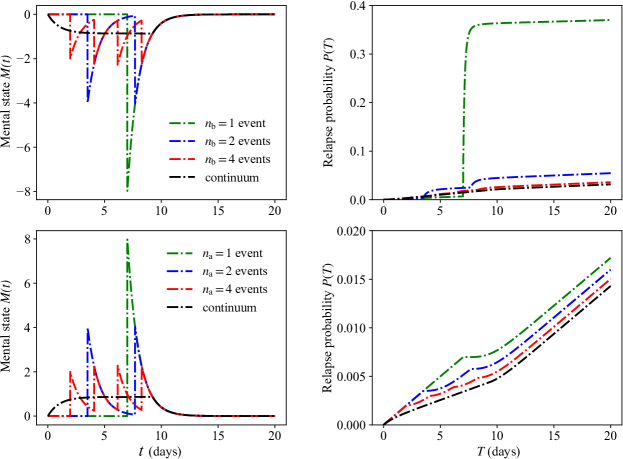
Figure 3: Top row: Mental state $M(t)$ and relapse probability $P(T)$ upon exposure to $n_{\rm b}=1,2,4$ negative events $\{-B_{i},t_{i}^{\rm b}\}$ and a continuum of stressors. All curves are obtained using Eqs. 1, 2, 4, and 12. Sequences define the same integrated mental state defined in Eq. 5 and are equivalent to the single event $\{-Z_{\rm b},t_{\rm b}\}$ shown in the red curve, where $Z_{\rm b}=8$ and $t_{\rm b}=7$ days. Within each sequence, events carry the same amplitude $B_{i}$ and are separated by the same time interval $\Delta_{\rm b}=$ 3.5 days ($n_{\rm b}=2$, black curve), 2 days ($n_{\rm b}=4$, blue curve), and 0.1 days (continuum, green curve). Other parameters are $\kappa_{\rm b}=1$/day,$~{}R_{0}=10^{-3}$/day,$~{}M_{0}=0$. Bottom row: Corresponding plots for sequences of equivalent positive events with $Z_{\rm a}=8$ and $t_{\rm a}=7$ days with $\kappa_{\rm a}=1$/day and $\Delta_{\rm a}=$ 3.5 days ($n_{\rm a}=2$, black curve), 2 days ($n_{\rm a}=4$, blue curve), and 0.1 days (continuum, green curve). Notice that for both positive and negative events the relapse probability is lowest for small events of limited magnitude.

We now study how external stimuli and intrinsic traits affect the relapse probability $P(T)$. External factors include specific realizations of the $\{A_{i},t_{i}^{\rm a}\}$ and $\{-B_{j},t_{j}^{\rm b}\}$ sequences, cue occurrence times $\{t_{\ell}^{\rm c}\}$ and drug availability profile $I(t)$. The intrinsic characteristics of an individual include how his or her mental state is affected by stressors, joyous events, and cues, the processing rates for positive and negative events, $\kappa_{\rm a}$ and $\kappa_{\rm b}$, for cues, $\kappa_{\rm c}$, and the intensity of the first high $w_{\rm peak}$. Relevant parameter ranges are listed in Table  1. Specifically, we measure time in units of days and fix $R_{0}=10^{-3}$/day consistent with known relapse rates of roughly 40 to 60 percent among opioid abuse disorder patients one year after treatment [51]. We assume drugs are always available and set $I(t)=1$ throughout the remainder of this work. Relapse is not possible if drugs are not available.

3.1 Dynamics without cues

We begin by studying the case of no cues and an unimpeded drug supply so that $C(t)=0$ and $I(t)=1$. We first analyze the simple case of a single life event and later consider sequences of multiple negative and positive ones. Our goal is to identify which combination of events (intensity and timing) leads to the smallest relapse likelihood.

3.1.1 Longer-lasting stressors increase the relapse probability; longer-lasting positive events decrease it

We consider a single stressor that is processed at three different rates $\kappa_{\rm b}$. Fig. 1 shows that the longer the stressor affects one’s mental state (i.e. the lower $\kappa_{\rm b}$), the larger the relapse probability $P(T)$. Corresponding results are shown for a positive experience processed at various rates $\kappa_{\rm a}$: lower values of $\kappa_{\rm a}$ result in smaller relapse likelihoods, as the effects of the positive event are retained for a longer time. Due to the exponential term in the relapse rate, stressors result in higher relapse likelihoods compared to positive ones of the same amplitude.

3.1.2 Clustered stressors increase the relapse probability more than disperse ones

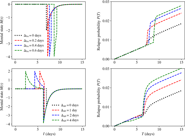
Figure 4: Top row: Mental state $M(t)$ and relapse probability $P(T)$ upon exposure to a stressor $\{-B_{1},t_{1}^{\rm b}\}$ followed by a positive event $\{A_{2},t_{2}^{\rm a}\}$. The two events are separated by lag times $\Delta_{\rm ba}=t_{2}^{\rm a}-t_{1}^{\rm b}=0,0.2,0.4,0.6$ hours. All curves are obtained using Eqs. 1, 2, 4, and 14. Parameters are $\kappa_{\rm b}=\kappa_{\rm a}=\kappa=1$/day, $B_{1}=4$, $A_{2}=2$, $~{}R_{0}=10^{-3}$/day,$~{}M_{0}=0$ and by setting $H=2e^{7}$. All event pairs define the same integrated mental state defined in Eq. 5 for $T>t_{2}^{\rm a}$. Notice that $P(T)$ increases with $\Delta_{\rm ba}$, implying that given a stressor, the likelihood of relapse is lowest the earlier a counteracting positive event occurs, in accordance with our analytical findings. Bottom row: Corresponding plots for a positive event $\{A_{1},t_{1}^{\rm a}\}$ followed by a stressor $\{-B_{2},t_{2}^{\rm b}\}$ with lag times $\Delta_{\rm ab}=t_{2}^{\rm b}-t_{1}^{\rm a}=0,1,2,4$ days with $A_{1}=2$, $B_{2}=4$ and all other parameters are the same as above. Here, $P(T)$ also increases with $\Delta_{\rm ab}$ and is smallest for $\Delta_{\rm ab}\to 0$.

We now include multiple life events and study how their timing affects the likelihood of relapse. Let us start with two negative events, $\{-B_{1},t_{1}^{\mathrm{b}}\}$ and $\{-B_{2},t_{2}^{\mathrm{b}}\}$, that define the time interval $\Delta_{\rm b}=t_{2}^{\mathrm{b}}-t_{1}^{\mathrm{b}}\geq 0$. We then define the effective time $U(T)$ given by

$$U(T) \equiv-\frac{\ln S(T)}{R_{0}}=\int_{0}^{T}e^{-M(s)}\mathrm{d}s$$ (10)

$$=t_{1}^{\rm b}+\!\int_{0}^{\Delta_{\rm b}}e^{B_{1}e^{-\kappa_{\rm b}s}}\mathrm{d}s+\!\int_{\Delta_{\rm b}}^{T-t_{1}^{\rm b}}\!\!e^{\left(B_{1}+B_{2}e^{\kappa_{\rm b}\Delta_{\rm b}}\right)e^{-\kappa_{\rm b}s}}\mathrm{d}s.$$

If $B_{1},B_{2}=0$ (as in the “neutral” case or baseline) Eq. 10 gives $U(T)=T$; finite values of $B_{1},B_{2}$ lead to $U(T)>T$, increasing the relapse probability $P(T)=1-S(T)$ above that of the baseline.

We now consider the family of paired events where the amplitudes $B_{1},B_{2}$ are fixed and where $t_{1}^{\rm b},t_{2}^{\rm b}$ are chosen such that for $T>t_{2}^{\rm b}$ the two events yield the same integrated mood as the single event $\{Z_{\rm b},t_{\rm b}\}$ defined in Eqs. 7. This implies that $B_{1}e^{\kappa_{\rm b}t_{1}^{\rm b}}+B_{2}e^{\kappa_{\rm b}t_{2}^{\rm b}}\equiv H_{\rm b}$ must be a constant, leaving one degree of freedom, which we choose to be $\Delta_{\rm b}$. The above constraints also impose that the integrated mental state, $\int_{0}^{T}M(s)\mathrm{d}s$ is invariant for all paired events within the family defined by $B_{1},B_{2},H_{\rm b}$. We may now ask: within this family of paired events, where the integrated mental state is fixed, which choice of $\Delta_{\rm b}$ minimizes the relapse probability at any time $T>t_{2}^{\rm b}$? We first express $t_{1}^{\rm b}$ in terms of $H_{\rm b}$ and $\Delta_{\rm b}$,

$$t^{\rm b}_{1}=\frac{1}{\kappa_{\rm b}}\ln\bigg{(}\frac{H_{\rm b}}{B_{1}+B_{2}e^{\kappa_{\rm b}\Delta_{\rm b}}}\bigg{)},$$ (11)

and make the dependence of $U(T)$ on $\Delta_{\rm b}$ explicit so that $U(T)\to U(T;\Delta_{\rm b})$ and

$$\kappa_{\rm b}U(T;\Delta_{\rm b})= \ln\Big{(}\frac{H_{\rm b}}{B_{1}+B_{2}e^{\kappa_{\rm b}\Delta_{\rm b}}}\Big{)}$$ (12)

$$\,\,+\mbox{ Ei}(B_{1})-\mbox{Ei}\big{(}B_{1}e^{-\kappa_{\rm b}\Delta_{\rm b}}\big{)}$$

$$\,\,+\mbox{ Ei}\big{(}B_{1}e^{-\kappa_{\rm b}\Delta_{\rm b}}+B_{2}\big{)}-\mbox{Ei}\big{(}H_{\rm b}e^{-\kappa_{\rm b}T}\big{)}$$

where the exponential integral $\mbox{Ei}(x)\equiv\int_{-\infty}^{x}t^{-1}e^{t}\mathrm{d}t$. Since $B_{1},B_{2},H_{\rm b}$ are fixed, the extrema of $U(T;\Delta_{\rm b})$ with respect to $\Delta_{\rm b}$ at any time $T$ are given by the zeros of

$$\kappa_{\rm b}\frac{\partial U(T;\Delta_{\rm b})}{\partial\Delta_{\rm b}}=(1-B_{2})e^{B_{1}e^{-\kappa_{\rm b}\Delta_{b}}}\!+\frac{e^{B_{2}}e^{B_{1}e^{-\kappa_{\rm b}\Delta_{b}}}\!-1}{1+\frac{B_{1}}{B_{2}}e^{-\kappa_{\rm b}\Delta_{\rm b}}}.$$ (13)

Regardless of $B_{1},B_{2},\kappa_{\rm b}$, the left hand side of Eq. 13 is a negative function of $\Delta_{\rm b}$, implying that $U(T;\Delta_{\rm b})$ has a maximum at $\Delta_{\rm b}\to 0$. Since $P(T)=1-S(T)=1-e^{-R_{0}U(T;\Delta_{\rm b})}$, we conclude that the largest relapse probability also occurs at $\Delta_{\rm b}\to 0$; that is, the relapse likelihood is largest when the two negative events occur simultaneously. In the top row of Fig. 2 we show the relapse probability $P(T)$ upon exposure to pairs of stressors that belong to the same family of events with fixed $B_{1},B_{2},H_{\rm b}$ and different timings $\Delta_{\rm b}$. The relapse probability is indeed largest when the time lag between the two stressors is smallest, $\Delta_{\rm b}\to 0$. We can apply the same arguments to more than two events and show that as the number of stressors increases, so does the likelihood of relapse. Given a negative integrated mental state generated by a set of $n_{\rm b}$ negative events occurring within time $T$, the relapse likelihood is largest when stressors are coincident, and is reduced when stressors are spread out. Fig. 3 shows the relapse probability for $n_{\rm b}=1,2,4$ and a continuum of negative events. In our model, relapse after a single catastrophic event is more likely than after a series of smaller stressors which cumulatively yield the same integrated negative mental state as the single catastrophic stressor.

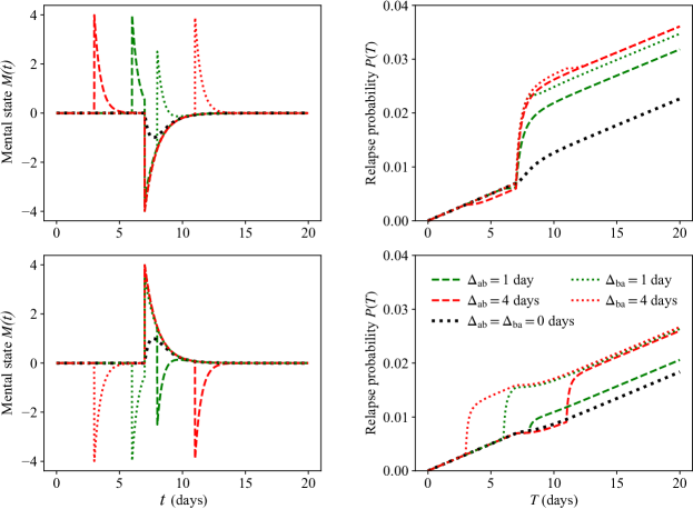
Figure 5: Top row: Mental state $M(t)$ and relapse probability $P(T)$ upon exposure to two events of opposite sign $\{A_{i},t_{i}^{\rm a}\}$ and $\{-B_{j},t_{j}^{\rm b}\}$ for $\kappa_{\rm a}=2$/day and $\kappa_{\rm b}=1$/day where $i=1,j=2$ or $j=1,i=2$. All curves are obtained using Eqs. 1, 2, 4, and 14. Events carry the amplitudes $A_{i}=B_{j}=4$; the other parameters are set at $M_{0}=0,R_{0}=10^{-3}$. Lag times are evaluated by setting $t_{j}^{\rm b}=7$ days where $j=1$ for lag times $\Delta_{\rm ba}=t_{2}^{\rm a}-t_{1}^{\rm b}$ and $j=2$ for lag times $\Delta_{\rm ab}=t_{2}^{\rm b}-t_{1}^{\rm a}$. For large enough $\Delta_{\rm ab}=\Delta_{\rm ba}=4$ days the relapse probability is independent of the order of events; however, for smaller lag times $\Delta_{\rm ab}=\Delta_{\rm ba}=1$ day, the order of events matters and the relapse probability is lower when the positive event $\{A_{1},t_{1}^{\rm a}\}$ occurs prior to the stressor $\{-B_{2},t_{2}^{\rm a}\}$. If the two events are concurrent and $\Delta_{\rm ab}=\Delta_{\rm ba}=0$ the total input to the mental state is negative since $\kappa_{\rm b}<\kappa_{\rm a}$ and the effects of the stressor are retained for a longer time than those of the positive event. Bottom row: Corresponding plots for $\kappa_{\rm a}=1$/day and $\kappa_{\rm b}=2$/day with all other parameters and events the same as those of the top row, and where the ordering of positive and negative events is reversed. Here, the order of events plays an even more crucial role when the time lag $\Delta_{\rm ab}=\Delta_{\rm ba}=1$ as the relapse probability is much lower when the positive event $\{A_{1},t_{1}^{\rm a}\}$ occurs prior to the stressor $\{-B_{2},t_{2}^{\rm a}\}$. Since $\kappa_{\rm b}\neq\kappa_{\rm a}$ it is not possible for the pairs of events to define the same mental state for all values of $t$.

3.1.3 Dispersed positive events decrease the relapse probability more than clustered ones

We can derive similar expressions to Eq. 10 for two positive life events for which the corresponding $U(T)$ is obtained by substituting $B_{1,2}\to-A_{1,2}$, and $t_{1}^{\rm b},\Delta_{\rm b},\kappa_{\rm b}\to t_{1}^{\rm a},\Delta_{\rm a},\kappa_{\rm a}$, respectively. Using the same methods as for pairs of negative events, we can show that the occurrence of two positive events decreases the likelihood of relapse the most when the two events are well spaced out. Results are shown in the bottom row of Fig. 2 for pairs of positive events with fixed $A_{1},A_{2},H_{\rm a}$ and different timings. The smallest likelihood of relapse occurs when the time lag between positive events $\Delta_{\rm a}$ is large, conversely, the likelihood of relapse is most pronounced for $\Delta_{\rm a}\to 0$. In the case of multiple, positive life events, as with the findings described for negative life events, the likelihood of relapse decreases the most when an individual experiences many distributed but moderately happy events, compared to a much larger but isolated positive episode that carries the same overall impact as the distributed ones. Results for sequences of multiple events belonging to the same family are shown in the bottom row of Fig. 3 for $n_{\rm a}=1,2,4$ where events are equally spaced and for a continuum of episodes. As expected, the lowest relapse probability occurs for a uniform distribution of positive events. A modest but continuous source of support is more protective against relapse than a very intense yet short-lived positive experience.

3.1.4 Relapse is least likely if a positive experience occurs immediately after a stressor

We now examine the case of a stressor $\{-B_{1},t_{1}^{\rm b}\}$ followed by a positive event $\{A_{2},t_{2}^{\rm a}\}$, where $t_{2}^{\rm a}>t_{1}^{\rm b}$. We label the positive event $A_{2}$ rather than $A_{1}$ so that it is clear that the positive event occurs after the negative one. Given an integrated mental state $\int_{0}^{T}M(t^{\prime})\mathrm{d}t^{\prime}$ and values for $B_{1},A_{2}$, the goal is to establish the lag time between the two events that minimizes the likelihood of relapse. The general case of different processing rates $\kappa_{\rm a}\neq\kappa_{\rm b}$ does not allow for easy generalization, so we set $\kappa_{\rm a}=\kappa_{\rm b}=\kappa$ to simplify our analysis. We write $U(T)=-\ln S(T)/R_{0}$ in terms of $\Delta_{\rm ba}=t_{2}^{\rm a}-t_{1}^{\rm b}$ and make the dependence on $\Delta_{\rm ba}$ explicit in the expression for $U(T;\Delta_{\rm ba})$ as follows

$$\kappa U(T;\Delta_{\rm ba})= \ln\bigg{(}\frac{H}{B_{1}-A_{2}e^{\kappa\,\Delta_{\rm ba}}}\bigg{)}$$ (14)

$$\,\,+\mbox{ Ei}(B_{1})-\mbox{Ei}(B_{1}e^{-\kappa\Delta_{\rm ba}})$$

$$\,\,+\mbox{ Ei}(B_{1}e^{-\kappa\Delta_{\rm ba}}-A_{2})-\mbox{Ei}(He^{-\kappa T}),$$

where $H\equiv B_{1}e^{\kappa t_{1}^{\rm b}}-A_{2}e^{\kappa t_{1}^{\rm a}}$ is a constant that ensures $\int_{0}^{T}M(t^{\prime})\mathrm{d}t^{\prime}$ is independent of $\Delta_{\rm ba}$. We can thus write

$$\kappa\frac{\partial U(T;\Delta_{\rm ba})}{\partial\Delta_{\rm ba}}= \,A_{2}e^{B_{1}e^{-\kappa\Delta_{\rm ba}}}$$ (15)

$$\,\,\times\Big{(}\frac{1-e^{-\kappa A_{2}}}{A_{2}}+\frac{e^{-B_{1}e^{-\kappa\Delta_{\rm ba}}}-e^{-\kappa A_{2}}}{B_{1}e^{-\kappa\Delta_{\rm ba}}-A_{2}}\Big{)}.$$

The left hand side of Eq. 15 is a positive function of $\Delta_{\rm ba}$ regardless of $A_{1},B_{2},\kappa$; as a consequence, for $T>t_{2}^{\rm a}$, $U(T;\Delta_{\rm ba})$ is an increasing function of $\Delta_{\rm ba}$ and attains its lowest value at $\Delta_{\rm ba}=0$. Thus, the relapse probability is also the lowest for $\Delta_{\rm ba}=0$. Once a negative life event occurs, the way to minimize the occurrence of relapses is for the individual to experience a healing, positive experience as soon as possible. Similar results hold in the case of a positive event $\{A_{1},t_{1}^{\rm a}\}$ followed by a negative event $\{B_{2},t_{2}^{\rm b}\}$; the relapse probability is lowest when the time lag between the two events is shortest.

In Fig. 4 we show the relapse probability for equivalent pairs of events $\{-B_{1},t_{1}^{\rm b}\}$ and $\{A_{2},t_{2}^{\rm a}\}$ that define a fixed $H\equiv B_{1}e^{\kappa t_{1}^{\rm b}}-A_{2}e^{\kappa t_{2}^{\rm a}}$ for $\kappa_{\rm a}=\kappa_{\rm b}=\kappa$. For large enough $T$, $P(T)$ decreases with $\Delta_{\rm ba}$, confirming our analytic predictions. The same finding arises for equivalent pairs of events $\{A_{1},t_{1}^{\rm a}\}$ and $\{-B_{2},t_{2}^{\rm b}\}$ that define a fixed $H\equiv-A_{1}e^{\kappa t_{1}^{\rm a}}+B_{2}e^{\kappa t_{2}^{\rm b}}$ for $\kappa_{\rm a}=\kappa_{\rm b}=\kappa$. To derive the mathematical results presented for pairs of events of amplitude $(A_{1},A_{2})$, $(B_{1},B_{2})$, $(B_{1},A_{2})$ and $(A_{1},B_{2})$ we assumed that no other prior events occurred; however, it is possible to show that our findings remain valid in the presence of earlier events. For example, given the events $\{A_{1},t_{1}^{\rm a}\}$, $\{-B_{2},t_{2}^{\rm b}\}$, $\{-B_{3},t_{3}^{\rm b}\}$ with $t_{3}^{\rm b}\geq t_{2}^{\rm b}\geq t_{1}^{\rm a}$ processed at the same rate $\kappa_{\rm a}=\kappa_{\rm b}=\kappa$ one can show that the relapse probability is still maximized upon clustering the two negative events $(B_{2},B_{3})$ and setting $\Delta_{\rm b}=t_{3}^{\rm b}-t_{2}^{\rm b}\to 0$.

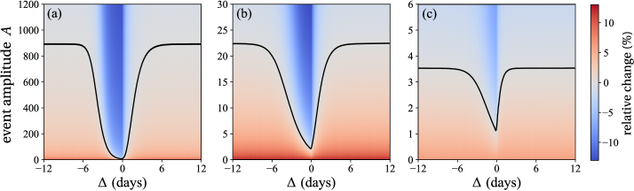
Figure 6: Long-term percentage changes in the relapse probability after one negative and one positive event relative to the neutral scenario of no events occurring. For $\Delta=\Delta_{\rm ba}=t_{2}^{\rm a}-t_{1}^{\rm b}>0$, the stressor $\{-B_{1},t_{1}^{\rm b}\}$ is followed by a positive event $\{A_{2},t_{2}^{\rm a}\}$ where $B_{1}=2$, $t_{1}^{\mathrm{b}}=12$ days and $A=A_{2}$ is determined from Eq. 17 at $T=30$ days. The color shading represents the percentage change of $P(T=30)$ assuming the two events have occurred relative to the neutral case. The black curve represents the amplitude of $A_{2}$ that yields the same relapse probability as the neutral case effectively neutralizing the effects of the stressor. For $\Delta=-\Delta_{\rm ab}=t_{1}^{\rm a}-t_{2}^{\rm b}<0$ the positive event $\{A_{1},t_{1}^{\rm a}\}$ is followed by a stressor $\{-B_{2},t_{2}^{\rm b}\}$ where $B_{2}=2$, $t_{2}^{\mathrm{b}}=12$ days. Here, the black curve tracks the amplitude of a preemptive positive event $A_{1}$ that would neutralize the future $B_{2}=2$ stressor at $T=30$ days as determined from Eq. 17. In panel (a) we set $\kappa_{\mathrm{a}}=2$/day, $\kappa_{\mathrm{b}}=1$/day; in panel (b) we set $\kappa_{\mathrm{a}}=\kappa_{\mathrm{b}}=1$/day; and in panel (c) we set $\kappa_{\mathrm{a}}=1$/day, $\kappa_{\mathrm{b}}=2$/day. The asymmetry between the positive and negative values of $\Delta$ underlines the importance of event order. For a given $\Delta=\Delta_{\rm ba}>0$, the value of $A_{2}$ necessary to balance $B_{1}=2$ is larger than the value of $A_{1}$ necessary to balance $B_{2}=2$ when $\Delta=-\Delta_{\rm ab}=-|\Delta_{\rm ba}|<0$. Upon comparing the black lines in the three panels for fixed $\Delta=\Delta_{\rm ba}>0$ the value of $A_{2}$ necessary to neutralize the $B_{1}$ stressor is larger when $\kappa_{\rm a}$ is larger or $\kappa_{\rm b}$ is lower, i.e. under fast processing of positive events or longer-lasting stressors. Similar considerations apply when $\Delta=\Delta_{\rm ab}<0$.

We now consider the general case $\kappa_{\rm a}\neq\kappa_{\rm b}$. In Fig. 5 we show results for pairs of events $\{A_{1},t_{1}^{\rm a}\}$ and $\{-B_{2},t_{2}^{\rm b}\}$ where $A_{1}=B_{2}$ and $\Delta_{\rm{ab}}\equiv t_{2}^{\rm b}-t_{1}^{\rm a}$, and for pairs of events $\{-B_{1},t_{1}^{\rm b}\}$ and $\{A_{2},t_{2}^{\rm a}\}$ where $B_{1}=A_{2}$ and $\Delta_{\rm ba}\equiv t_{2}^{\rm a}-t_{1}^{\rm b}$. The long-term relapse probability $P(T)$ is largely insensitive to the absolute timing of the pair of events, as long as $T-t_{2}^{\mathrm{a,b}}\gg\kappa_{\mathrm{a}}^{-1},\kappa_{\mathrm{b}}^{-1}$; however, it strongly depends on the event order and the magnitude of the time lag $\Delta_{\rm ab}$ or $\Delta_{\rm ba}$. For a fixed $\Delta_{\rm ab}=\Delta_{\rm ba}$, $P(T)$ may depend significantly on the order of events. In general, the larger $\kappa_{\rm a}\Delta_{\rm ab}$ and $\kappa_{\rm b}\Delta_{\rm ba}$, the less sensitive the relapse probability is to the order of events as shown by comparing the cases $\Delta_{\rm ab}=\Delta_{\rm ba}=4$ days with $\Delta_{\rm ab}=\Delta_{\rm ba}=1$ day in Fig. 5. Note that since $\kappa_{\rm a}\neq\kappa_{\rm b}$ it is impossible for the pairs of events in Fig. 5 to define the same integrated mental state $\int_{0}^{T}M(t^{\prime})\mathrm{d}t^{\prime}$ for any given $T$.

Finally, given a stressor $\{-B_{1},t_{1}^{\rm b}\}$ which is processed at a rate $\kappa_{\rm b}$ we determine which later event $\{A_{2},t_{2}^{\rm a}\}$ processed at rate $\kappa_{\rm a}$ will yield the same relapse probability as the baseline case, where no events occur. To do this, we note that under the baseline, $U(T)=T$ and that since it is not possible to define a single event as in Eq. 14 for $\kappa_{\rm a}\neq\kappa_{\rm b}$, we must write $U(T;\Delta_{\rm ba})$ in its general form

$$U(T;\Delta_{\rm ba})=t_{1}^{\rm b}+\int_{0}^{\Delta_{\rm ba}}e^{B_{1}e^{-\kappa_{\rm b}t}}\mathrm{d}t+\int_{\Delta_{\rm ba}}^{T-t_{1}^{\rm b}}\!\!e^{B_{1}e^{-\kappa_{\rm b}t^{\prime}}-A_{2}e^{-\kappa_{\rm a}(t^{\prime}-\Delta_{\rm ba})}}\mathrm{d}t^{\prime}$$ (16)

where $\Delta_{\rm ba}=t_{2}^{\rm a}-t_{1}^{\rm b}$. To find the value of $A_{2}$ that balances $U(T;\Delta_{\rm ba})$ with the baseline $U(T)=T$, we must solve

$$U(T;\Delta_{\rm ba})= \,t_{1}^{\rm b}+\frac{1}{\kappa_{\rm b}}\left[\rm{Ei}(B_{1})-\rm{Ei}\left(B_{1}e^{-\kappa_{\rm b}\Delta_{\rm ba}}\right)\right]$$ (17)

$$\,+\frac{1}{\kappa_{\rm a}}\left[\rm{Ei}(-A_{2})-\rm{Ei}\big{(}-A_{2}e^{-\kappa_{\rm a}(T-t_{1}^{\rm b}-\Delta_{\rm ba})}\big{)}\right]$$

$$= U(T)=T.$$

Under the assumption $\kappa_{\rm a}\Delta_{\rm ba},\kappa_{\rm b}\Delta_{\rm ba}\gg 1$, and using the identity $\lim_{x\rightarrow 0}{\rm Ei}(x)=\ln|x|+\gamma$, where $\gamma$ is the Euler-Mascheroni constant, Eq. 17 can be simplified to

$$\rm{Ei}(-A_{2})-\gamma-\ln(A_{2})=\frac{\kappa_{\rm a}}{\kappa_{\rm b}}\big{[}\ln(B_{1})+\gamma-\rm{Ei}(B_{1})\big{]}.$$ (18)

Eq. 18 yields the value of $A_{2}$ that neutralizes the effects of a stressor of amplitude $B_{1}$ so that at long times the relapse rate is the same as if neither event occurred. It is straightforward to show that upon substituting $B_{1}\to-A_{1}$ and $A_{2}\to-B_{1}$ Eq. 18 still holds when the order of events is reversed and the positive event occurs prior to the negative one. The black curves in Fig. 6 trace the values of $A=A_{2}$ that balance a stressor of amplitude $B_{1}$ given a lag time $\Delta=\Delta_{\rm ba}>0$ for various choices of $\kappa_{\rm a}$ and $\kappa_{\rm b}$. These results correspond to positive values of $\Delta$. Vice-versa, the amplitude of a protective event $A=A_{1}$ that can balance a later stressor of amplitude $B_{2}$ are shown for negative values of $\Delta=-\Delta_{\rm ab}<0$. The asymmetry between positive and negative values of $\Delta$ for all choices of $\kappa_{\rm a}$ and $\kappa_{\rm b}$ implies that a modest amplitude of the positive event is required to balance a fixed stressor, regardless of whether the positive event occurs before or after the stressor. The other color-coded regions in Fig. 6 show the percent increase (or decrease) of the relapse probability $P(T)$ compared to the neutral case of no negative or positive life event, for specific values of $A_{1},A_{2},B_{1},B_{2},t_{1}^{\rm a},t_{1}^{\rm b},t_{2}^{\rm a},t_{2}^{\rm b},T,\kappa_{\rm a},\kappa_{\rm b}$.

3.1.5 A constant source of positivity can offset the random lows of life

We now study the scenario in which there is a constant input $Y$ to the mental state which may represent a continuous stressor or source of support. We also assume that positive and negative life events occur randomly and are processed at rates $\kappa_{\rm a}=\kappa_{\rm b}=\kappa$. Under these assumptions we describe the dynamics for $M=M_{\rm a}+M_{\rm b}$ as

$$\frac{\mathrm{d}M}{\mathrm{d}t}=-\kappa M+Y+\xi(t),$$ (19)

where $\xi(t)$ is a Gaussian white noise term that represents the random, positive and negative, life events. We set the general initial mental state value $M(t=0)=M_{0}$ and write the mean and correlation function of $\xi(t)$ as

$$\langle\xi(t)\rangle= 0$$ (20)

$$\langle\xi(t)\xi(t^{\prime})\rangle= 2\lambda\delta(t-t^{\prime}).$$

Eqs. 20 define an Ornstein-Uhlenbeck stochastic process, a classic paradigm in statistical mechanics [52, 53, 54, 55]. The relapse rate of the neutral case, where there are no life events or continuous inputs to perturb an individual’s mental state and $Y=\xi(t)=0$, is given by

$$R_{\rm d}(t)=R_{0}e^{-M_{0}e^{-\kappa t}}.$$ (21)

If $Y\neq 0$ and $\xi(t)\neq 0$, Eq. 19 can be solved as

$$M(t)= \mu_{\rm m}(t)+\int_{0}^{t}\!e^{-\kappa(t-t^{\prime})}\xi(t^{\prime})\mathrm{d}t^{\prime},$$ (22)

$$\mu_{\rm m}(t)\equiv \frac{Y}{\kappa}+\Big{(}M_{0}-\frac{Y}{\kappa}\Big{)}e^{-\kappa t}.$$

Associated with Eqs. 19 and 20 is a Fokker-Planck equation governing the dynamics of the probability density function $P_{\rm m}(M,t)$ [54, 53]

$$\frac{\partial P_{\rm m}(M,t)}{\partial t}=\frac{\partial}{\partial M}\Big{(}(\kappa M-Y)P_{\rm m}\Big{)}+\lambda\frac{\partial^{2}P_{\rm m}}{\partial M^{2}}.$$ (23)

The solution to Eq. 23 and the initial condition $P(M,t=0)=\delta(M-M_{0})$ is

$$P_{\rm m}(M,t)= \frac{1}{\sqrt{2\pi\sigma_{\rm m}^{2}(t)}}e^{-\frac{(M-\mu_{M}(t))^{2}}{2\sigma_{\rm m}^{2}(t)}}$$ (24)

$$\sigma^{2}_{\rm m}(t)\equiv \frac{\lambda}{k}(1-e^{-2kt}).$$

In the limit $t\to\infty$, Eq. 24 defines a steady state Gaussian distribution centered at $Y/\kappa$ with variance $\lambda/\kappa$. The expected time-dependent relapse rate is given by

$$\langle R(t)\rangle=R_{0}\langle e^{-M(t)}\rangle=R_{0}\!\int_{-\infty}^{\infty}\!\!\!e^{-M}P(M,t)\mathrm{d}M$$ (25)

which is explicitly expressed as

$$\langle R(t)\rangle= R_{0}\exp\Big{[}-\mu_{\rm m}(t)+\frac{1}{2}\sigma_{\rm m}^{2}(t)\Big{]},$$ (26a)

$$\langle R(t\to\infty)\rangle= R_{0}\exp\Big{[}\frac{(\lambda-2Y)}{2\kappa}\Big{]}.$$ (26b)

The relapse rate in Eq. 26b can be compared with the equivalent expression obtained in the absence of noise, i.e. for $Y\neq 0$ and $\xi(t)=\lambda=0$

$$\frac{\langle R(t\to\infty)\rangle}{R(t\to\infty;\xi(t)=0)}=e^{\lambda/2\kappa}>1.$$ (27)

Since the above $\lambda$-independent ratio is always larger than one, Eq. 27 implies that unbiased noise, where positive and negative life events are equally likely in frequency and magnitude, results in a larger relapse rate than the noise-free case, regardless of the sign of $Y$. Mathematically, this result stems from the asymmetry in $R_{0}e^{-M(t)}$ where the increase due to a stressor is much larger than the decrease following a positive fluctuation of similar amplitude, consistent with the brain’s negativity bias [44]. We can also compare the general case $Y\neq 0$ and $\xi(t)\neq 0$ with the neutral case $Y=\xi(t)=0$ yielding

$$\frac{\langle R(t\to\infty)\rangle}{R_{\rm d}(t\to\infty)}=\exp\Big{[}\frac{(\lambda-2Y)}{2\kappa}\Big{]}.$$ (28)

The values of $Y,\lambda$ in Eq. 28 can be tuned so that the driving term and the noise balance each other. Specifically, for the long term expected relapse rate in the presence of noise to be less than the relapse rate in the absence of any external input, the constant input $Y$ must obey $Y>\lambda/2$. Given the form for $P(T)$ in Eq. 2, we can write the expected relapse probability as

$$\langle P(T)\rangle=1-\left\langle\exp\Big{[}-R_{0}\int_{0}^{T}e^{-M(t)}\mathrm{d}t\Big{]}\right\rangle$$ (29)

and approximate it in the $\kappa T\gg 1$ limit by

$$\langle P(T)\rangle \approx 1-\exp\Big{[}-R_{0}\int_{0}^{T}\langle e^{-M(t)}\rangle\mathrm{d}t\Big{]}$$ (30)

$$\approx 1-\exp\Big{[}-e^{\frac{\lambda-2Y}{2\kappa}}R_{0}T\Big{]}.$$

In the Appendix we discuss Eq. 29 and cases where the approximation in Eq. 30 fails, namely in the $\kappa\to 0$ limit. Fig. 7 shows the expected relapse rate $\langle R(t)\rangle$ as $\kappa,Y,\lambda$ are varied. Results derived from 100,000 simulations of the stochastic process in Eq. 19 are compared with predictions from the analytical result (Eq. 26a). We also show the relapse rate for the baseline given by $R_{\rm d}(t)=R_{0}$. The expected relapse rate increases with the noise amplitude $\lambda$ and decreases with the magnitude of the positive experience $Y$ and with the processing rate $\kappa$. Lower $\kappa$ values imply longer processing times for all events; however, since the asymmetry in $R(t)$ assigns more weight to negative occurrences, a larger likelihood of relapse is observed as $\kappa\to 0$. The corresponding values of the expected relapse probability $\langle P(T)\rangle$ obtained from simulations and from the analytical approximation in Eq. 30 are shown in Fig. 8.

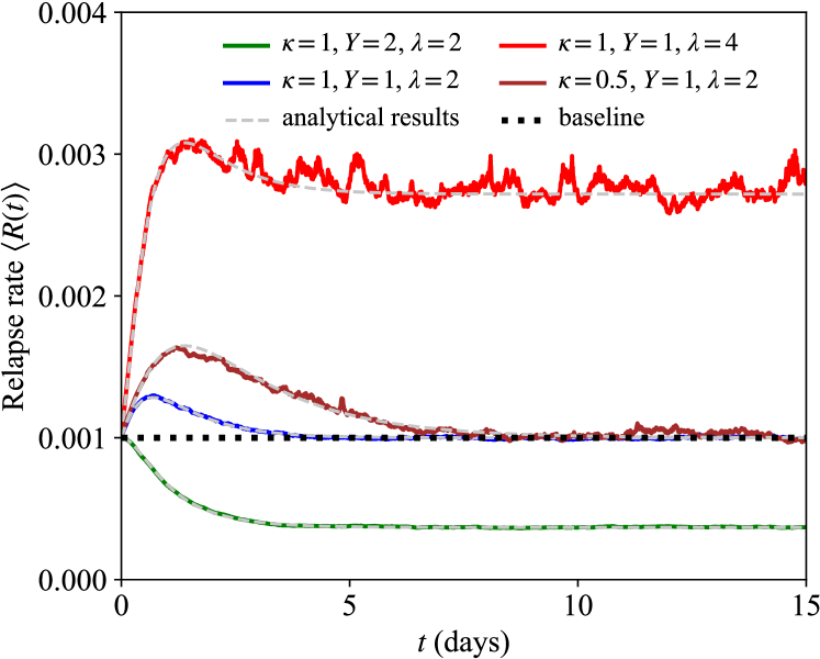
Figure 7: Dynamics of $\langle R(t)\rangle$ averaged over 100,000 realizations of the Ornstein-Uhlenbeck described by Eq. 19 and the analytical expression for $\langle R(t)\rangle$ in Eq. 26a. Parameters are $M_{0}=0,R_{0}=10^{-3}$/day. Values in the legend are in units of /day. For $\lambda=2Y$ the $t\to\infty$ relapse rate in Eq. 26b $\langle R(t\to\infty)\rangle=R_{0}$ matches the neutral case of no exposure to any positive or negative life event.

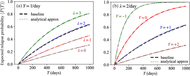
Figure 8: Expected relapse probability $\langle P(T)\rangle$ as derived from averaging over 5,000 realizations of the Ornstein-Uhlenbeck process in Eq. 19 and the analytical approximation in Eq. 30 for the baseline $Y=\lambda=0$ with $R_{0}=10^{-3},\kappa=1$/day. Values of $\lambda,Y$ displayed along the curves are in units of /day. In panel (a) we set $Y=1$/day; as $\lambda$ is increased $\langle P(T)\rangle$ also increases. For $\lambda=2Y$ results from the baseline are recovered. Small values of $\lambda<2Y$ decease $\langle P(T)\rangle$ below the baseline, whereas large fluctuations $\lambda>2Y$ increase $\langle P(T)\rangle$ beyond the baseline. In panel (b) we set $\lambda=2$/day and allow $Y$ to be negative, representing constant negative experiences that increase $\langle P(T)\rangle$. These results indicate that sustained, large enough positive experiences may neutralize a series of random, potentially large stressors.

Finally, we evaluate the first passage statistics to a given mental state $M_{\rm th}<0$. Although the threshold level value can be arbitrary, we set it to be negative to represent a critically unhappy mental state. The dynamics of the mean first passage time $T_{\rm m}(M)$ to reach $M_{\rm th}$ starting from a given mental state $M>M_{\rm th}$ can be derived from the backward Kolmogorov equation associated with Eq. 23

$$\lambda\frac{\mathrm{d}^{2}T_{\rm m}}{\mathrm{d}M^{2}}-(\kappa M-Y)\frac{\mathrm{d}T_{\rm m}}{\mathrm{d}M}=-1$$ (31)

along with absorbing boundary conditions $T\,(M_{\rm th})=0$ and $T_{\rm m}\,(M\to\infty)=0$. Equation 31 can be solved using standard methods to yield

$$T_{\rm m}(M)=\frac{\sqrt{\pi}}{\kappa}\int_{\sqrt{\frac{\kappa}{2\lambda}}(M_{\rm th}-Y/\kappa)}^{\sqrt{\frac{\kappa}{2\lambda}}(M-Y/\kappa)}\!e^{z^{2}}{\rm{erfc}}(z)\mathrm{d}z$$ (32)

where ${\rm erfc}(x)$ is the complementary error function ${\rm erfc}(x)=1-{\rm{erf}}(x)$. Since the argument of the integrand is a positive, decreasing function of $z$, Eq. 32 implies that $T_{\rm m}(M)$ is increasing in $Y,M$ and decreasing in $\lambda,M_{\rm th}$. This is to be expected, given that large values of $Y,M$ tend to shift the mental state away from the lower negative threshold $M_{\rm th}$, and given that large $\lambda$ values lead to larger fluctuations that are more likely to reach the negative $M_{\rm th}$. However, $T_{\rm m}(M)$ is non-monotonic with $\kappa$ as shown in the top row of Fig. 9. Here we plot $T_{\rm m}(M=0)$ as derived from Eq. 32 and denote it as $T_{\rm m}(M=0\to M=M_{\rm th})$ for clarity. Note that $T_{\rm m}(M=0)$ decreases with increasing $\kappa$ at low values of $\kappa$ and increases with $\kappa$ at large $\kappa$. To understand this non-monotonicity, note that the mental state $M$ will be restored towards $Y/\kappa$ within a time frame $\kappa^{-1}$ after any random fluctuation. As $\kappa\to\infty$, this implies that after each random event, $M\to 0$ very quickly and that cumulative effects of multiple past random events will be very limited. As a result, increasing $\kappa$ when $\kappa$ is already large will make reaching $M_{\rm th}$ less likely and thus, the mean first passage time will increase.

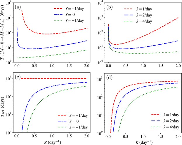
Figure 9: Top row: Mean first passage time $T_{\rm m}(M=0\to M=M_{\rm th})$ for an initial mental state $M=0$ to reach the negative threshold $M_{\rm th}=-2$ as a function of the decay rate $\kappa$. Results follow from the random process in Eq. 19 and the analytical form in Eq. 32. For large $\kappa$, each random fluctuation dissipates quickly so that the effects of multiple inputs to the mental state do not accumulate appreciably, hence $T_{\rm m}(M)$ increases with $\kappa$. Increasing $\kappa$ for small values of $\kappa$ will reduce the likelihood of positive values of the mental state thus shortening the time to reach $M_{\rm th}$ as discussed in the text. These two trends lead to the observed non-monotonic behavior, which is most pronounced for large $Y,\lambda$. In (a) we set $\lambda=2$/day and vary the constant input $Y$; in (b) we set $Y=0$ and vary the noise amplitude $\lambda$. Bottom row: Mean first passage time $T_{\rm rel}$ to relapse computed from the approximation in Eq. 35 and shown as a function of the decay rate $\kappa$. In panel (c) we set $\lambda=2$/day and vary the constant input $Y$; in panel (d) we set $Y=0$ and vary the noise amplitude $\lambda$.

On the other hand, when $\kappa\approx 0$, $M$ will grow approximately linearly away from $M_{\rm th}$ driven by the $Y$ input while being subject to noise. Whatever the initial value of $M$, for large enough values of $Y$ and $\lambda$, $M$ will most likely become positive before one, or a sequence of, negative random events will lead it close to $M_{\rm th}$. Increasing $\kappa>0$ will now lessen any positive values of $M$, and thus accelerate reaching the $M_{\rm th}$ threshold. Any negative values of $M$ will instead increase as $\kappa$ is increased, and this will cause a delay in hitting $M_{\rm th}$. However, given the negative value of the threshold, excursions in the $M>0$ space will be much longer than those in the $0<M<M_{\rm th}$ space, so that acceleration in reaching $M_{\rm th}$ will dominate. As a result, increasing $\kappa$ when $\kappa$ is small will lead to a shorter mean first passage time. This effect will be more pronounced for large values of $Y,\lambda$ as the excursion to, and permanence in, the $M>0$ space will be more sustained in these cases. When $Y,\lambda$ are small and especially if the initial $M$ value is negative, decreases in $T_{\rm m}(M)$ as $\kappa$ is increased for small values of $\kappa$ will be much less evident, as excursions to the $M>0$ plane will be rare. An alternate representation of Eq. 32 is given by expanding the integrand via a Taylor series and evaluating the integral, leading to

$$T_{\rm m}(M)= \frac{\pi}{2\kappa}{\rm erfi}(z_{\rm in})-\frac{z_{\rm in}^{2}}{\kappa}{{}_{2}}F_{2}\Big{(}1,1;\frac{3}{2},2;z_{\rm in}^{2}\Big{)}$$ (33)

$$-\frac{\pi}{2\kappa}{\rm erfi}(z_{\rm eg})+\frac{z_{\rm eg}^{2}}{\kappa}{{}_{2}}F_{2}\Big{(}1,1;\frac{3}{2},2;z_{\rm eg}^{2}\Big{)}$$

where ${{}_{2}}F_{2}$ is the generalized hypergeometric function and

$$z_{\rm in}=\sqrt{\frac{\kappa}{2\lambda}}\Big{(}M-\frac{Y}{\kappa}\Big{)},\,\,\,z_{\rm eg}=\sqrt{\frac{\kappa}{2\lambda}}\Big{(}M_{\rm th}-\frac{Y}{\kappa}\Big{)}.$$ (34)

Eqs. 32 and 33 are the mean time $T_{\rm m}(M)$ for an initial mental state $M$ to first reach the threshold $M_{\rm th}$; one may similarly determine the mean first time to relapse $T_{\rm{rel}}$ using Eq. 2

$$T_{\rm{rel}}=\int_{0}^{\infty}\langle S(T)\rangle\mathrm{d}T\approx\frac{e^{\frac{2Y-\lambda}{2\kappa}}}{R_{0}}.$$ (35)

The last relationship arises from Eq. 30 and is valid for $\kappa T\gg 1$. We show $T_{\rm{rel}}$ as a function of $\kappa$ in the bottom row of Fig. 9, using the same parameters chosen for $T_{\rm{m}}(M)$. The mean first time to relapse is an increasing function of $Y$ and a decreasing function of $\lambda$, indicating that positive continuous inputs and exposure to relatively small noise amplitudes can act as protective factors. These trends are consistent with those observed for $T_{\rm{m}}(M)$.

3.2 The presence of cues

In this section, we study how cues affect the mental state and the likelihood of relapse. According to Eqs. 1 and 9 sensory cues are mathematically represented as a stressor of fixed amplitude $w_{\rm peak}$ occurring at times $t_{\ell}^{\rm c}$. This description is consistent with psychiatric studies that have identified overlaps in the neural circuits that process stress and drug-related cues and that have found that both lead to cravings and heightened susceptibility to relapse [56, 49]. As mentioned earlier, we assume that cues always bring back memories of the first high so that the amplitude $w_{\rm peak}$ is fixed. As a result, findings illustrated in Sections 3.1.1 and 3.1.4 still hold upon substituting $B_{i}\to w_{\rm peak}$ for all $i$ and $\kappa_{\rm b}\to\kappa_{\rm c}$. In particular, relapse is less likely if a positive experience occurs immediately after being exposed to a drug-related cue and one can still utilize the results shown in Fig. 6 to determine the magnitude and timing of the positive experience necessary to balance exposure to a cue. Values of $\kappa_{\rm c}$ will be chosen such that $\kappa_{\rm c}>\kappa_{\rm b}$, as we expect the time to process a drug-related cue to be less than the time to overcome a stressor.

Consider the case in which an individual is randomly exposed, through a Poisson process with rate $\lambda_{\rm c}$, to cues that elicit the memory of the first high. The individual thus experiences, with probability $P_{\rm c}(n_{\rm c},t)=(\lambda_{\rm c}t)^{n_{\rm c}}e^{-\lambda_{\rm c}t}/n_{\rm c}!$, $n_{\rm c}$ cues within a time interval $t$. The mean time between successive cues is $1/\lambda_{\rm c}$. Given the equivalence between cues and stressors, these results may also be interpreted as the response to an identical stressor presented at random, Poisson-distributed times. The dynamics of the cue-induced motivation is thus

$$\frac{\mathrm{d}C}{\mathrm{d}t}=-\kappa_{\rm c}C+w_{\rm peak}\sum_{\ell=1;t\geq t^{\rm c}_{\ell}}^{n_{\rm c}}\delta(t-t^{\rm c}_{\ell}),$$ (36)

where $n_{\rm c}$ are the Poisson-distributed number of events that have occurred until time $t$. We also assume that there is a counteracting source of support $Y>0$ to the mental state so that

$$M(t)=M_{\rm a}(t)=\frac{Y}{\kappa_{\rm a}}\big{(}1-e^{-\kappa_{\rm a}t}\big{)}.$$ (37)

We solve Eq. 36 with the initial condition $C(t=0)=0$. The resulting expression for $C(t)$ can be used to write the relapse rate $R(t)$ in Eq. 1 using the mental state $M(t)=M_{\rm a}(t)$ given in Eq. 37 and under the assumption that drugs are fully available $I(t)=1$. We find

$$\frac{R(t)}{R_{0}}=e^{-\frac{Y}{\kappa_{\rm a}}\left(1-e^{-\kappa_{\rm a}t}\right)}\!\!\prod_{\ell=1;t\geq t^{\rm c}_{\ell}}^{n_{\rm c}}\!\!e^{w_{\rm peak}e^{-\kappa_{\rm c}\left(t-t_{\ell}^{\rm c}\right)}.}$$ (38)

Using well known properties of the Poisson process shown in the Appendix we estimate the expected value of the relapse rate for any number of events occurring within time $t$ as

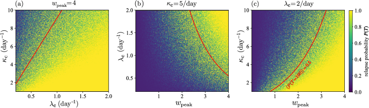
Figure 10: Relapse probability $P(T=100)$ following exposure to a single, randomly drawn sequence of sensory cues occurring at times generated according to a Poisson process of rate $\lambda_{\mathrm{c}}$. The corresponding relapse rate is evaluated through Eq. 38 and the relapse probability at $T=100$ days, $P(T=100)$, is evaluated using Eqs. 2. The red curves depict the analytical approximation obtained for $\langle P(T=100)\rangle=0.5$ calculated using Eqs. 40 and 41. We do not include any positive, continuous form of support so that $Y=0$ and results are independent of the processing rate $\kappa_{\rm a}$. In panel (a) we fix $w_{\rm peak}=4$; in panel (b) we fix $\kappa_{\mathrm{c}}=5$/day; in panel (c) we fix $\lambda_{\mathrm{c}}=2$/day. Collectively, the panels show that the likelihood of relapse increases with increases in the amplitude $w_{\mathrm{peak}}$, the frequency of cue occurrences $\lambda_{\mathrm{c}}$, or the typical cue processing time $1/\kappa_{\mathrm{c}}$.

$$\left\langle{\frac{R(t)}{R_{0}}}\right\rangle= \exp\left({-\lambda_{\rm c}t-\frac{Y}{\kappa_{\rm a}}(1-e^{-\kappa_{\rm a}t})}\right)$$ (39)

$$\,\,\,\times\exp\Big{[}\lambda_{\rm c}\int_{0}^{t}e^{w_{\rm peak}e^{-\kappa_{\rm c}\left(t-t^{\prime}\right)}}\mathrm{d}t^{\prime}\Big{]}.$$

In the $\kappa_{\rm a}t,\kappa_{\rm c}t\gg 1$ limit Eq. 39 can be approximated by

$$\ln\Big{\langle}{\frac{R(t)}{R_{0}}}\Big{\rangle}\approx-\displaystyle{\frac{Y}{\kappa_{\rm a}}+\frac{\lambda_{\rm c}}{\kappa_{\rm c}}}\big{(}{\rm Ei}(w_{\rm peak})-\ln(w_{\rm peak})-\gamma\big{)},$$ (40)

where $\gamma$ is the Euler-Mascheroni constant. We use the approximation in Eq. 40 to evaluate the relapse rate $R(t)$ in Eq. 2, leading to an approximate expression for $\langle P(T)\rangle$, valid for $\kappa_{\rm a}T,\kappa_{\rm c}T\gg 1$

$$\langle P(T)\rangle=1-\langle e^{-\int_{0}^{T}R(t){\rm d}t}\rangle\approx 1-e^{-R_{0}Te^{Q_{\rm c}}},$$ (41)

where

$$Q_{\rm c}\equiv-\displaystyle{\frac{Y}{\kappa_{\rm a}}+\frac{\lambda_{\rm c}}{\kappa_{\rm c}}}\big{(}{\rm Ei}(w_{\rm peak})-\ln(w_{\rm peak})-\gamma\big{)}.$$ (42)

In Fig. 10, we evaluate the probability of relapse at given values $\kappa_{\rm c},\lambda_{\rm c},w_{\rm peak}$. We do this by first drawing a sequence of cues that occur according to a Poisson process of rate $\lambda_{\rm c}$. Then, using this specific sequence of cues, we compute the relapse rate given in Eq. 38. Finally, we determine the survival probability and the relapse probability at a fixed time $T=100$ days using Eqs. 2. The results in Fig. 10 are obtained under the assumption of no positive input, $Y=0$. For comparison we use the analytical approximation given in Eqs. 40 and 41 to find the parameter curve corresponding to $\langle P(T=100)\rangle=0.5$.

In the baseline case, where there are no cues or external stimuli, $R(t)=R_{0}$, hence the positive support $Y$ will balance or alleviate the cue-induced drive to take drugs only if it satisfies

$$Y\geq\frac{\lambda_{\rm c}\kappa_{\rm a}}{\kappa_{\rm c}}\big{(}{\rm Ei}(w_{\rm peak})-\ln(w_{\rm peak})-\gamma\big{)}.$$ (43)

Thus, to be effective, the counterbalancing source of support $Y$ must increase with the intensity of the memory of the first high $w_{\rm peak}$, the rate of exposure to the cues $\lambda_{\rm c}$, the duration of the cue $1/\kappa_{\rm c}$ and the processing rate of the positive events $\kappa_{\rm a}$.

4 Conclusions

We presented a mathematical model for the probability of relapse in drug addiction. Our model incorporates dynamics that reflect psychiatric concepts such as the positive activation, negative activation (PA/NA) model and the peak-end rule.

Addiction research, like other studies that focus on learning, memory, rewards and synaptic plasticity, relies on neuroimaging methods to understand how the brain and its neurocircuitry adapt to short- or long-term drug use and ensuing behavioral changes. It is well documented that drug users and former users display dysregulation in their brain reward system, heightened reactivity to drug-related cues and stressors, less inhibitory self-control, and a tendency to engage in compulsive behaviors. It is also well established that the process of physical detoxification is a relatively short one, but cravings and relapse can occur even long after cessation of drug use. Relapse is often triggered by exposure to stressors or drug-related cues that the former user is unable to manage. Among the biggest limitations of neuroimaging studies and clinical trials are the need to control for individual predispositions and external circumstances, high costs, difficulties in recruiting volunteers with substance use disorder especially in longitudinal studies.

Given the complexities of addiction and the practical limitations in obtaining comprehensive data, simple and analytically tractable mathematical models may be helpful to understand how the brain responds to drugs and their absence. Decision-making and many psychiatric disorders, including addiction, have been described using quantitative mathematical models in recent years [57, 58, 59, 60, 61, 62]. In our work, we considered the response of the brain to a series of inputs representing positive and negative events, and how their amplitude, timing and ordering affect the likelihood that a person in recovery will use again. By construction, and mirroring the PA/NA model, negative events increase the likelihood of relapse more than positive ones of the same magnitude. We find that clustering positive or negative events is generally detrimental. For a fixed, mental state activity integrated over a fixed time frame and imparted by an arbitrary number of negative (or positive) events, the best way of distributing these events is through a continuum of moderate negativity (or positivity), rather than as a large jolt of catastrophe (or happiness) occurring at all once. On the other hand, once an individual is exposed to a stressor, a positive event occurring immediately afterward can act as a protective factor. We also found that a constant source of positive input can balance the negativity arising from a series of random events that may include large stressors. Since the mathematical representation of sensory cues in our work is akin to that of stressors, the above considerations remain valid for exposure to drug-related cues.

The effect of different environments and user profiles may be studied by tuning relevant parameters. By changing $\kappa_{\rm a},\kappa_{\rm b},\kappa_{\rm c}$ and $w_{\rm peak}$ we can represent users who respond differently to life experiences and whose memories of the “first high” vary in intensity. Similarly, the amplitudes $A_{i},B_{j}$, the Gaussian noise $\lambda$ and the Poisson parameter $\lambda_{\rm c}$ can represent different risk levels in the social environment of the recovering addict. Finally, although developed in the context of relapse, our model can be used to also study the driving and protective factors that lead a non-user to try drugs for the first time. In this case, $C(t)=0$ as there are no sensory cues related to past use, but $M(t)$ can represent external stimuli that induce an individual to use drugs for the first time.

How do we translate these findings into practice? How to experience continuous positivity? Certainly, it is important to seek out positive, fulfilling experiences, embodied by the $A_{i}$ events discussed in this work. However, the continuous sources of positivity we introduced, such as the green curves in Fig. 3 and the $Y$ term in Eq. 19, represent inputs to the mental state. One may interpret these inputs as arising not just from actual events, but also as imparted from a positive attitude towards life, for example through support from family and friends, finding satisfaction in one’s work, hobbies and social life. A positive attitude can also be developed through cognitive behavioral therapy, individual or group counseling or psychotherapy which are known to be effective in helping manage life’s challenges without recourse to drugs.

SYMBOL	QUANTITY	RANGE
$M_{\rm a}$	positive activity of the mental state	$\sim 10$
$M_{\rm b}$	negative activity of the mental state	$\sim-10$
$C$	mental response to cues	$\sim 1$
$\kappa_{\rm a},~{}\kappa_{\rm b}$	equilibration values of the mental state processing rates	$\sim 1$/day
$\kappa_{\rm a,0},~{}\kappa_{\rm b,0}$	onset values of the mental state processing rates	$0.6\sim 0.8\kappa_{\rm{a,b}}$ [63]
$\gamma_{\rm a},~{}\gamma_{\rm b}$	recovery rates for $\kappa_{\rm a}(t)$ and $\kappa_{\rm b}(t)$	$0.002\sim 0.02$/day [63]
$\kappa_{\rm c}$	processing rates of drug-related cues and memories	$\sim 10$/day
$R_{0}$	rate of relapse in the neutral mental state (without inputs)	$\sim 10^{-3}$/day
$A_{i}$	intensity of positive life event i	$\sim 1$
$B_{j}$	intensity of negative life event j	$\sim 1$
$w_{\mathrm{peak}}$	intensity of most pleasurable drug-taking reward response	$\sim 1$
$t_{i}^{\mathrm{a}}$	time of occurrence of positive life event i	$\sim$ day
$t_{j}^{\mathrm{b}}$	time of occurrence of negative life event j	$\sim$ day
$t_{\ell}^{\mathrm{q}}$	time of occurrence of cue $\ell$	$\sim$ day
$\lambda_{q}$	Poisson process rate for the occurrence of cues	$\sim 1$/day
$Y$	continuous input to the mental state
$\kappa$	mental state processing rate for $\kappa_{\rm a}=\kappa_{\rm b}$
$\lambda$	Gaussian noise intensity in the OU process for the mental state

Table 1: Relevant quantities and parameter ranges for the relapse models presented in Eqs. 1, 3a, 3b (distinct mental state neurocircuitry for few positive and negative events, no cues); Eqs. 1, 19, (common mental state neurocircuitry for random, Gaussian distributed positive and negative events, no cues); Eqs. 1, 9, 36, 37 (distinct mental state neurocircuitry for uniform, positive events, subject to Poisson distributed drug-related cues) and time-dependent forms for the processing rates.

5 Acknowledgement

M.R.D. and T. C. acknowledge support from the Army Research Office through grant W911NF-18-1-0345.

6 Appendix

Appendix A Time-dependent processing rates $\kappa_{\rm a}(t)$ and $\kappa_{\rm b}(t)$

Time-dependent processing rates $\kappa_{\rm a}(t)$, $\kappa_{\rm b}(t)$ are included in our mathematical representations of the PA/NA model in Eqs. 3a and 3b to allow for neuroadaptive changes after cessation of drug use. Assuming that at the beginning of the recovery phase at $t=0$ there are no negative or positive affects so that $M_{\rm a}(t=0)=M_{\rm b}(t=0)=0$, the general solution is

$$M_{\rm a}(t)= \sum_{i,t\geq t_{i}^{\rm a}}A_{i}e^{-\int_{t_{i}^{\rm a}}^{t}\kappa_{\rm a}(s^{\prime}){\rm d}s^{\prime}},$$ (44a)

$$M_{\rm b}(t)= -\sum_{j,t\geq t_{j}^{\rm b}}B_{j}e^{-\int_{t_{j}^{\rm b}}^{t}\kappa_{\rm b}(s^{\prime}){\rm d}s^{\prime}}$$ (44b)

Drug addiction is known to attenuate the pleasure stemming from positive stimuli, leading to anhedonia [27]. It is thus reasonable to assume that after cessation of drug use, positive experiences will return to being more pleasurable. This is supported by experimental evidence that dopamine transporter loss in former methamphetamine users can recover after a sufficiently long period of abstinence [63]. Plausible forms for $\kappa_{\rm a}(t)$ include monotonically decreasing functions that start at $\kappa_{\rm a}(t=0)=\kappa_{\rm a,0}$ and that descend towards the standard value at full recovery $\kappa_{\rm a}(t\to\infty)=\kappa_{\rm a}^{*}<\kappa_{\rm a,0}$. Within this scenario, positive events occurring well into the recovery phase elevate one’s mental state for a longer period compared to positive events occurring at the onset of the recovery phase. Similarly, since drug abuse is known to exacerbate negative emotional distress [25, 47, 48, 64], we can assume that $\kappa_{\rm b}(t)$ is a monotonically increasing function with $\kappa_{\rm b}(t=0)=\kappa_{\rm b,0}$ that increases towards $\kappa_{\rm b}(t\to\infty)=\kappa_{\rm b}^{*}>\kappa_{\rm b,0}$. In this case, negative affects linger less in the minds of former users as recovery continues. We mathematically represent the processing rates $\kappa_{\rm a}(t),\kappa_{\rm b}(t)$ during abstinence as

$$\kappa_{\rm a}(t)= \kappa_{\rm a,0}e^{-\gamma_{\rm a}t}+\kappa_{\rm a^{*}}(1-e^{-\gamma_{\rm a}t}),$$ (45a)

$$\kappa_{\rm b}(t)= \kappa_{\rm b,0}e^{-\gamma_{\rm b}t}+\kappa_{\rm b^{*}}(1-e^{-\gamma_{\rm b}t}),$$ (45b)

where $\gamma_{\rm a}^{-1},\gamma_{\rm b}^{-1}$ are typical time scales associated with neuroadaptive changes to the processing rates and where $\kappa_{\rm a,0}>\kappa_{\rm a}^{*}$ and $\kappa_{\rm b,0}<\kappa_{\rm b}^{*}$. The positive affect $M_{\rm a}(t)$ in Eq. 44a can thus be written as

$$M_{\rm a}(t)=\sum_{i,t\geq t_{i}^{\rm a}}A_{i}e^{-\kappa^{*}_{\rm a}(t-t_{i}^{\rm a})}\exp\left[\frac{(\kappa_{\rm a}^{*}-\kappa_{\rm a,0})}{\gamma_{\rm a}}\left(e^{-\gamma_{\rm a}t_{i}^{\rm a}}-e^{-\gamma_{\rm a}t}\right)\right].$$ (46)

For $M_{\rm b}(t)$ in Eq. 44b instead we find

$$M_{\rm b}(t)=-\sum_{j,t\geq t_{j}^{\rm b}}B_{j}e^{-\kappa^{*}_{\rm b}(t-t_{j}^{\rm b})}\exp\left[\frac{(\kappa_{\rm b}^{*}-\kappa_{\rm b,0})}{\gamma_{\rm b}}\left(e^{-\gamma_{\rm b}t_{j}^{\rm b}}-e^{-\gamma_{\rm b}t}\right)\right].$$ (47)

If the restoring, neuroadaptive changes to $\kappa_{\rm a}(t)$ occur over short time scales such that $\gamma_{\rm a}t_{i}^{\rm a}\gg 1$, then $\kappa_{\rm a}(t)$ can be approximated by its equilibration value $\kappa_{\rm a}^{*}$. Conversely, for longer lived changes scales such that $\gamma_{\rm a}t_{i}^{\rm a}\ll 1$, then $\kappa_{\rm a}(t)$ can be approximated by its initial condition $\kappa_{\rm a,0}$. In either of these two limits, $\kappa_{\rm a}(t)$ can be approximated by a constant, $\kappa_{\rm a}$. Similar considerations hold for $\kappa_{\rm b}(t)$ that in the same limits can be modeled as a constant $\kappa_{\rm b}$. We can thus write

$$M_{\rm a}(t)=\sum_{i,t\geq t_{i}^{\rm a}}A_{i}e^{-\kappa_{\rm a}(t-t_{i}^{\rm a})},\quad M_{\rm b}(t)=-\sum_{j,t\geq t_{j}^{\rm b}}B_{j}e^{-\kappa_{\rm a}(t-t_{j}^{\rm b})},$$ (48)

where $\kappa_{\rm a}=\kappa_{\rm a,0}$ or $\kappa_{\rm a}^{*}$ depending on the proper limit (and similarly for $\kappa_{\rm b}$) and use the results for the constant $\kappa_{\rm a},\kappa_{\rm b}$ cases discussed in Eqs. 4.

Instead of considering a sequence of positive or negative events, for simplicity, we now assume there is a constant negative input $Y=-0.5$/day and that there are no random events. In this scenario, the ideal case of an individual who has never used drugs is represented by the negative mental state $M(t)=M_{\rm b}(t)$ given by

$$M(t)=\frac{Y}{\kappa^{*}_{\rm b}}(1-e^{-\kappa_{\rm b}^{*}t}),$$ (49)

and obtained using the standard processing rate $\kappa^{*}_{\rm b}$. We identify the scenario of a recovering addict processing events with the same rates as if drugs were never used, as a proxy for full recovery. A patient still in recovery on the other hand processes events at the time-dependent rate $\kappa_{\rm b}(t)$ given by Eq. 45b. For this individual, the same circumstances yield the following negative mental state

$$M(t)=Ye^{-\int_{0}^{t}\kappa_{\rm b}(t^{\prime}){\rm d}t^{\prime}}\int_{0}^{t}e^{\int_{0}^{t^{\prime}}\kappa_{\rm b}(t^{\prime\prime}){\rm d}t^{\prime\prime}}\mathrm{d}t^{\prime}$$ (50)

Eq. 50 reduces to Eq. 49 under no recovery, when $\gamma_{\rm b}=0$ in Eq. 50, provided $\kappa^{*}_{\rm b}$ is replaced by $\kappa_{\rm b,0}$ in Eq. 49.

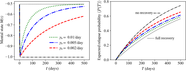
Figure 11: Dynamics of $M(t)$ and $\langle P(T)\rangle$ under a continuous negative input $Y=-0.5$/day, an initial processing rate $\kappa_{{\rm b},0}=1$/day, a fully recovered processing rate $\kappa_{\rm b}^{*}=2$/day, and $R_{0}=10^{-3}$. Recovery rates are given by $\gamma_{\mathrm{b}}=0.002,0.005,0.01$/day. The black dashed curve is the ideal case of the individual never having used drugs, or having fully recovered (Eq. 49), and the dotted curve is the no recovery case ($\gamma_{\rm b}=0$ in Eq. 50). Intermediate curves show patients in recovery who tend to approach the ideal case of never having drugs after a long enough recovery time.

In Fig. 11 we consider a dynamically varying $\kappa_{\rm b}(t)$ and plot the mental state $M(t)$ and relapse probability $P(t)$ for an initial processing rate $\kappa_{0,\rm b}=1$/day and the recovered, standard processing rate $\kappa^{*}_{\rm b}=2$/day. The initially large value of $\kappa_{0,\rm b}$ implies that right after cessation of drug use the neurocircuitry of the individual is still compromised, and any life event is processed quickly. We also set $\gamma_{\rm b}=0.002$/day, $\gamma_{\rm b}=0.005$/day and $\gamma_{\rm b}=0.01$/day, corresponding to recovery times from $\kappa_{0,\rm b}$ to $\kappa^{*}_{\rm b}$ ranging from three months to one and half years, approximately.

The mental states $M(t)$ in each of these scenarios are shown in Fig. 11(a). In Fig. 11(b) we show the corresponding expected relapse probability, $\langle P(T)\rangle$. Here, the state of no exposure to drugs (Eq. 49) is represented by the lower-bounded curve and the state of no recovery from drugs (Eq. 50 with $\gamma_{\rm b}=0$) is represented by the upper-bounded one. All other curves correspond to Eq. 50 with finite, non-zero values of the recovery rate $\gamma_{\rm b}$. As can be seen, the latter are all initially closer to the upper bound, as the recovery effects are minimal at the onset. However, as the recovery process continues, the curves start approaching the lower curve corresponding to the ideal case of the individual never having used drugs in the first place. Finally, faster recovery processes (larger values of $\gamma_{\rm b}$) yield lower relapse probabilities.

Appendix B Estimating the relapse probability

Here, we consider approximations to the expected relapse probability $\langle P(T)\rangle$ as given by Eq. 29

$$\langle P(T)\rangle=1-\langle S(T)\rangle=1-\left\langle\exp\left[-R_{0}\int_{0}^{T}e^{-M(t^{\prime})}\mathrm{d}t^{\prime}\right]\right\rangle.$$ (51)

We first expand the exponential in Eq. 51 in a Taylor series

$$\langle S(T)\rangle=\sum_{n=0}^{\infty}\frac{R_{0}^{n}}{n!}(-1)^{n}\int_{0}^{T}\!\!\cdots\!\int_{0}^{T}\!\langle e^{-M(t^{(1)})}\!\cdots e^{-M(t^{(n)})}\rangle\mathrm{d}t^{(1)}\!\cdots\mathrm{d}t^{(n)}$$ (52)

and note that upon neglecting correlations we can approximate the expectation of the products of $e^{-M(t)}$ in Eq. 52 as products of expectations so that

$$\int_{0}^{T}\!\!\cdots\!\int_{0}^{T}\langle e^{-M(t^{(1)})}\cdots e^{-M(t^{(n)})}\rangle\mathrm{d}t^{(1)}\!\cdots\mathrm{d}t^{(n)}\approx\left[\int_{0}^{T}\langle e^{-M(t)}\rangle\mathrm{d}t\right]^{n}$$ (53)

leading to

$$\langle P(T)\rangle\approx 1-\exp\bigg{[}-R_{0}\int_{0}^{T}\langle e^{-M(t)}\rangle\mathrm{d}t\bigg{]}.$$ (54)

We now evaluate the integral for the $n=1$ summand in Eq. 52, for which Eq. 53 is exact. We find

$$\langle e^{-M(t)}\rangle =\int_{-\infty}^{\infty}\!\!e^{-M}P_{\rm m}(M,t)\,\mathrm{d}M$$ (55)

$$=\exp{\left(\frac{\lambda-2Y}{2\kappa}\right)}\exp{\left[-\left(M_{0}-\frac{Y}{\kappa}\right)e^{-\kappa t}-\frac{\lambda}{2\kappa}e^{-2\kappa t}\right]}.$$

We now consider the $n=2$ summand in Eq. 52 to determine the conditions under which the approximation in Eq. 53 fails and correlations must be taken into account. Our goal is thus to evaluate $\langle e^{-M(t^{(1)})}e^{-M(t^{(2)})}\rangle\equiv\langle e^{-M(t^{\prime})}e^{-M(t^{\prime\prime})}\rangle$. To do this, we must consider the joint probability density $P_{\rm m}(M_{1},M_{2},t^{\prime},t^{\prime\prime})$ of finding the mental state $M_{1}$ at time $t^{\prime}$ and of finding the mental state $M_{2}$ at time $t^{\prime\prime}>t^{\prime}$, conditioned on the previous value $M_{1}$ at time $t^{\prime}$ This is given by

$$P_{\rm m}(M_{1},M_{2},t^{\prime},t^{\prime\prime})=P_{\rm m}(M_{2},t^{\prime\prime}|M_{1},t^{\prime})P_{\rm m}(M_{1},t^{\prime})$$ (56)

where $P_{\rm m}(M_{1},t^{\prime})$ is the probability density of finding $M_{1}$ at $t^{\prime}$, with the given initial conditions, and where $P_{\rm m}(M_{2},t^{\prime}|M_{1},t^{\prime})$ is the probability density of finding $M_{2}$ at $t^{\prime\prime}$, conditioned on having $M_{1}$ at $t^{\prime}$. The two quantities evolve according to the Fokker-Planck equation shown in Eq. 23 and lead to

$$\langle e^{-M(t^{\prime})} e^{-M(t^{\prime\prime})}\rangle$$ (57)

$$=\int_{-\infty}^{\infty}\int_{-\infty}^{\infty}\!e^{-M_{1}}e^{-M_{2}}P_{\rm m}(M_{2},M_{1},t^{\prime},t^{\prime\prime})\mathrm{d}M_{1}\mathrm{d}M_{2}$$

$$=\int_{-\infty}^{\infty}\int_{-\infty}^{\infty}\!e^{-M_{1}}e^{-M_{2}}P_{\rm m}(M_{2},t^{\prime\prime}|M_{1},t^{\prime})P_{\rm m}(M_{1},t^{\prime})\mathrm{d}M_{1}\mathrm{d}M_{2}$$

where

$$P_{\rm m}(M_{1},t^{\prime})\sim {\cal N}\left(\mu_{1}(t^{\prime}),~{}\sigma^{2}(t^{\prime})\right)$$ (58)

$$P_{\rm m}(M_{2},t^{\prime\prime}|M_{1},t^{\prime})\sim {\cal N}\left(\mu_{2}(t^{\prime\prime}-t^{\prime}),~{}\sigma^{2}(t^{\prime\prime}-t^{\prime})\right)$$

and ${\cal N}(\mu,\sigma)$ is the normal distribution of mean $\mu$ and variance $\sigma$. The values $\mu_{1},\mu_{2},\sigma$ are given by

$$\mu_{1}(t^{\prime})= \frac{Y}{\kappa}+\left(M_{0}-\frac{Y}{\kappa}\right)e^{-\kappa t^{\prime}}$$ (59)

$$\mu_{2}(t^{\prime\prime}-t^{\prime})= \frac{Y}{\kappa}+\left(M_{1}-\frac{Y}{\kappa}\right)e^{-\kappa(t^{\prime\prime}-t^{\prime})}$$

$$\sigma^{2}(t)= \frac{\lambda}{\kappa}(1-e^{-2\kappa t}).$$

We now evaluate Eq. 57 to find

$$\langle e^{-M(t^{\prime})}e^{-M(t^{\prime\prime})}\rangle= \langle e^{-M(t^{\prime})}\rangle\langle e^{-M(t^{\prime\prime})}\rangle e^{\frac{2\lambda}{\kappa}e^{-\kappa t^{\prime\prime}}\sinh(\kappa t^{\prime})}$$ (60)

where $\langle e^{-M(t^{\prime})}\rangle$ is given in Eq. 55.

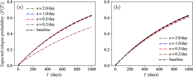
Figure 12: Expected relapse probability $\langle P(T)\rangle$ as determined from 5,000 trajectories of the Ornstein-Uhlenbeck process with $M_{0}=0$ and various parameters $Y,\lambda,\kappa$ and the analytical estimate given by Eqs. 26a and 30. The ratio $\lambda=2Y$ is kept for all parameter combinations, leading to the expectation $\langle P(T)\rangle\approx 1-\exp(R_{0}T)$, according to Eq. 30. In panel (a) we fix $Y=1$/day and $\lambda=2$/day. Results from the numerical simulations match the analytical estimate only for large values of $\kappa$ as illustrated in the text, when correlations can be neglected. In panel (b) we fix $2\lambda=\alpha\kappa$, with $\alpha=8$ to show that under this assumption correlations play a less prominent role in the limit $\kappa\to 0$.

Given that $t^{\prime\prime}>t^{\prime}$, the exponential term in Eq. 60 will tend towards unity as $\kappa\to\infty$, implying correlations can be neglected. The $\kappa\to\infty$ limit corresponds to a relatively short processing time, consistent with the notion that the decay of random events is fast and do not allow for strong correlations. Conversely, if $\kappa\to 0$ we find

$$\lim_{\kappa\to 0}\exp\left(\frac{2\lambda}{\kappa}e^{-\kappa t^{\prime\prime}}\sinh(\kappa t^{\prime})\right)=e^{2\lambda t^{\prime}}$$ (61)

which can be quite large for even moderate values of $\lambda$ at large times. Finally, note that if we set $2\lambda=\alpha\kappa$ where $\alpha$ is a proportionality constant, then

$$\lim_{\kappa\to 0}\exp\left(\alpha e^{-\kappa t^{\prime\prime}}\sinh(\kappa t^{\prime})\right)=1,$$ (62)

suggesting that an alternative way of neglecting correlations in the small $\kappa$ limit, when the processing time is large, is to instead modulate the amplitude of the noise $\lambda$ to be comparable to $\kappa$. The evaluation of higher order correlations $n>2$ in Eq. 52 is a more tedious calculation, but we expect that in the $\kappa\to\infty$ limit the same considerations will apply and that correlations can also be neglected. In Fig. 12 we plot the expected relapse probability $\langle P(T)\rangle$ obtained by averaging over 5,000 runs of the Ornstein-Uhlenbeck process for several values of $\kappa$ and other parameters. We show that the analytical approximation in Eq. 30 holds only for sufficiently large values of $\kappa$.

Appendix C Deriving the average relapse rate for Poisson distributed cues

We now derive Eq. 39 assuming cues affect the mental state $M$ through events of amplitude $w_{\rm peak}$ that are Poisson distributed with rate $\lambda_{\rm c}$. According to Eq. 38, assuming that within time $t$ there have been $n_{\rm c}$ Poisson distributed cues, the relapse rate is given by

$$\frac{R(t)}{R_{0}}=\exp\left[-\frac{Y}{\kappa_{\rm a}}\left(1-e^{-\kappa_{\rm a}t}\right)\right]\!\prod_{\ell=1;t\geq t^{\rm c}_{\ell}}^{n_{\rm c}}\!\!\!\exp\left[w_{\rm peak}e^{-\kappa_{\rm c}\left(t-t_{\ell}^{\rm c}\right)}\right].$$ (63)

For a general function $f(y)$ one can show that given $n_{\rm c}$ events within time $t$ that are Poisson distributed, the following holds

$$\left.\left\langle\prod_{\ell=1}^{n_{\rm c}}f(t^{\rm c}_{\ell})\right\rangle\right|_{n_{\rm c}}\!\!=\left[\frac{1}{t}\int_{0}^{t}f(y)\mathrm{d}y\right]^{n_{\rm c}}\quad\,n_{\rm c}\sim\mathrm{Poisson}(\lambda_{\rm c},t).$$ (64)

We will show the validity of this expression below. For now, assuming Eq. 64 holds, we write

$$\left.\left\langle\frac{R(t)}{R_{0}}\right\rangle\right\rvert_{n_{\rm c}}=\exp\left[-\frac{Y}{\kappa_{\rm a}}\left(1-e^{-\kappa_{\rm a}t}\right)\right]\left[\frac{1}{t}\int_{0}^{t}\exp\left[w_{\rm peak}e^{-\kappa_{\rm c}\left(t-t^{\prime}\right)}\right]\mathrm{d}t^{\prime}\right]^{n_{\rm c}}.$$ (65)

We can now average over the likelihood of having $n_{\rm c}$ events within $t$ by weighting Eq. 65 by the Poisson distribution to obtain

$$\left\langle\frac{R(t)}{R_{0}}\right\rangle= \exp\left[-\frac{Y}{\kappa_{\rm a}}\left(1-e^{-\kappa_{\rm a}t}\right)\right]$$ (66)

$$\times\sum_{n_{\rm c}=0}^{\infty}\frac{(\lambda_{\rm c}t)^{n_{\rm c}}e^{-\lambda_{\rm c}t}}{n_{\rm c}!}\left[\frac{1}{t}\int_{0}^{t}\exp\left[w_{\rm peak}e^{-\kappa_{\rm c}\left(t-t^{\prime}\right)}\right]\mathrm{d}t^{\prime}\right]^{n_{\rm c}}$$

Upon evaluating the integral we can write

$$\left\langle\frac{R(t)}{R_{0}}\right\rangle= \exp\left[-\lambda_{\rm c}t-\frac{Y}{\kappa_{\rm a}}\left(1-e^{-\kappa_{\rm a}t}\right)\right]$$ (67)

$$\times\exp\left[\lambda_{\rm c}\int_{0}^{t}e^{w_{\rm peak}e^{-\kappa_{\rm c}\left(t-t^{\prime}\right)}}\mathrm{d}t^{\prime}\right]$$

which, for $\kappa_{\rm a}t,\kappa_{\rm c}t\gg 1$ can be simplified to

$$\lim_{t\rightarrow\infty}\ln\left\langle\frac{R(t)}{R_{0}}\right\rangle=-\frac{Y}{\kappa_{\rm a}}+\frac{\lambda_{\rm c}}{\kappa_{\rm c}}\left({\rm Ei}(w_{\rm peak})-\ln(w_{\rm peak})-\gamma\right)$$ (68)

where $\gamma$ is the Euler-Mascheroni constant. To show the validity of Eq. 64 we take a general Poisson process of rate $\eta$ and for which $p(t_{1},\ldots,t_{n}|N=n)$ is the probability density of $n$ events occurring within time $t$ ordered such that $t_{1}\leq t_{2}\leq\dots\leq t_{n}$. In a Poisson process, the possibility of an event occurring in $[t,t+\mathrm{d}t]$ is always $\eta\mathrm{d}t$, which does not correlate with time, so we can divide the time period $t$ equally into $M$ segments of length $\mathrm{d}t$ with $M\gg 1$ so that $t=M\mathrm{d}t$. We label them $\{[T_{1},T_{1}+\mathrm{d}t],[T_{2},T_{2}+\mathrm{d}t],\ldots,[T_{M},T_{M}+\mathrm{d}t]\}$. Since each event $t_{1}\leq t_{k}\leq t_{n}$ will fall into one of the above segments we can write

$$p(t_{1},\ldots,t_{n}| N=n)(\mathrm{d}t)^{n}$$ (69)

$$=\mathbb{P}(T_{1}<t_{1}<T_{1}+\mathrm{d}t,\ldots,T_{n}<t_{n}<T_{n}+\mathrm{d}t)$$

$$=\mathbb{P}(\{[T_{1},T_{1}+\mathrm{d}t],\ldots,[T_{n},T_{n}+\mathrm{d}t]\})$$

where the last equality implies that one can simply pick the $n\in M$ segments corresponding to the $t_{1}\leq t_{k}\leq t_{n}$ events. Since these intervals are equiprobable, and

$$p(t_{1},\ldots,t_{n}|N=n)(\mathrm{d}t)^{n}=\binom{M}{n}^{-1}=\frac{n!(M-n)!}{M!}\approx\frac{n!}{M^{n}}.$$

Using $M=t/\mathrm{d}t$, this becomes $p(t_{1},\ldots,t_{n}|N=n)=\frac{n!}{t^{n}}$. An alternative way to obtain this is result is to use the explicit form for the Poisson distribution

$$p(t_{1},\ldots,t_{n}|N=n)= \frac{p(t_{1},\ldots,t_{n},N=n)}{P(N=n)}$$ (70)

$$= \frac{e^{-\eta(T-t_{n})}\cdot\eta e^{-\eta(t_{n-1}-t_{n})}\cdots\eta e^{-\eta(t_{1}-t_{2})}\cdot\eta e^{-\eta t_{1}}}{\frac{(\eta T)^{n}e^{-\eta T}}{n!}}$$

$$= \frac{\eta^{n}e^{-\eta T}}{\frac{(\eta T)^{n}e^{-\eta T}}{n!}}=\frac{n!}{T^{n}}.$$

Finally, for a generic function $f(t)$ and for a series of $n$ Poisson-distributed events occurring at times $0<t_{1}<\dots<t_{n}<t$ we can write

$$\left.\left\langle\prod_{j=1}^{n}f(t_{j})\right\rangle\right|_{n} =\int\left[\prod_{j=1}^{n}f(t_{j})p(t_{1},\ldots,t_{n}|N=n)\right]\mathrm{d}t_{1}\cdots\mathrm{d}t_{n}$$

$$=\frac{n!}{t^{n}}\int\left[\prod_{j=1}^{n}f(t_{j})\right]\mathrm{d}t_{1}\cdots\mathrm{d}t_{n}=\frac{n!}{t^{n}}\int\left[\prod_{j=1}^{n}f(t_{j})\mathrm{d}t_{j}\right],$$

where the multidimensional time integrals are constrained by $0<t_{1}<\dots<t_{n}<t$. We now eliminate the ordering of the sequence $t_{1},\ldots,t_{n}$, and divide the integral by the number of permutations to obtain

$$\left.\left\langle\prod_{j=1}^{n}f(t_{j})\right\rangle\right|_{n} =\frac{1}{t^{n}}\left[\prod_{j=1}^{n}\int_{0<t_{j}<t}f(t_{j})\mathrm{d}t_{j}\right]$$

$$=\prod_{j=1}^{n}\left[\int_{0}^{t}f(t_{j})\frac{\mathrm{d}t_{j}}{t}\right]=\frac{1}{t}\left[\int_{0}^{t}f(y)\mathrm{d}y\right]^{n},$$

which is Eq. 64.

References

- [1] Farida Bhuiya Ahmad, Jodi A. Cisewski, Lauren M. Rossen, and Paul Sutton. Provisional drug overdose death counts. National Center for Health Statistics, 2022.
- [2] U.S. Department of Health and Human Services, Substance Abuse and Mental Health Services Administration, Center for Behavioral Health Statistics and Quality, NSDUH-2021-DS0001. National Survey on Drug Use and Health 2021. https://datafiles.samhsa.gov, 2021.
- [3] Nora D. Volkow and Marisela Morales. The brain on drugs: From reward to addiction. Cell, 162(4):712–725, 2015.
- [4] National Institute on Drug Abuse. Treatment and recovery. https://nida.nih.gov/publications/drugs-brains-behavior-science-addiction/treatment-recovery, 2022.
- [5] A. Thomas McLellan, David C. Lewis, Charles P. O’ Brien, and Herbert D. Kleber. Drug dependence, a chronic medical illness: Implications for treatment, insurance, and outcomes evaluation. Journal of the American Medical Association, 284:1689–1695, 2000.
- [6] Rajita Sinha. New findings on biological factors predicting addiction relapse vulnerability. Current Psychiatry Reports, 13:398–405, 2011.
- [7] Mary L. Brecht and Diane Herbeck. Time to relapse following treatment for methamphetamine use: a long-term perspective on patterns and predictors. Drug and Alcohol Dependence, 139:18–25, 2014.
- [8] Bobby P. Smyth, Joseph Barry, Eamon Keenan, and Kevin Ducray. Lapse and relapse following inpatient treatment of opiate dependence. Irish Medical Journal, 103:176–179, 2010.
- [9] Alan David Kaye, Richard D. Urman, Elyse M. Cornett Cornett, and Amber Edinoff. Substance Use and Addiction Research: Methodology, Mechanisms, and Therapeutics. Academic Press, London, UK, 2023.
- [10] Maria R. D’Orsogna, Lucas Böttcher, and Tom Chou. Fentanyl-driven acceleration of racial, gender and geographical disparities in drug overdose deaths in the United States. PLOS Global Public Health, 3:e0000769, 2023.
- [11] Daniele Caprioli, Michele Celentano, Giovanna Paolone, and Aldo Baldiani. Modeling the role of environment in addiction. Progress in Neuro-Psychopharmacology and Biological Psychiatry, 31:1639–1653, 2007.
- [12] Nora D. Volkow, Joanna S. Fowler, and Gene-Jack Wang. The addicted human brain: insights from imaging studies. The Journal of Clinical Investigation, 111:1444–1451, 2003.
- [13] George F. Koob and Nora D. Volkow. Neurocircuitry of addiction. Neuropsychopharmacology: official publication of the American College of Neuropsychopharmacology, 35(1):217–238, jan 2010.
- [14] Rita Z. Goldstein and Nora D. Volkow. Dysfunction of the prefrontal cortex in addiction: neuroimaging findings and clinical implications. Nature Reviews Neuroscience, 12(11):652–669, 2011.
- [15] George F. Koob and Nora D. Volkow. Neurobiology of addiction: a neurocircuitry analysis. The Lancet. Psychiatry, 3:760–773, 2016.
- [16] Jessica A. Mollick and Hedy Kober. Computational models of drug use and addiction: A review. Journal of Abnormal Psychology, 129:544–555, 2020.
- [17] Tom Chou and Maria R. D’Orsogna. A mathematical model of reward-mediated learning in drug addiction. Chaos, 32:021102, 2022.
- [18] Boris S. Gutkin, Stanislas Dehaene, and Jean P. Changeux. A neurocomputational hypothesis for nicotine addiction. Proceedings of the National Academy of Sciences, 103:1106–1111, 2006.
- [19] Abraham Peper. Intermittent adaptation: A mathematical model of drug tolerance, dependence and addiction. In Boris S. Gutkin and Serge H. Ahmed, editors, Computational Neuroscience of Drug Addiction, Springer Series in Computational Neuroscience, volume 10, chapter 2, pages 19–56. Springer, New York, NY, 2012.
- [20] Hawre Jalal, Jeanine M. Buchanich, Mark S. Roberts, Lauren C. Balmert Balmert, Kun Zhang Zhang, and Donald S. Burke. Changing dynamics of the drug overdose epidemic in the United States from 1979 through 2016. Science, 361:6408, 2018.
- [21] Lucas Böttcher, Tom Chou, and Maria R. D’Orsogna. Modeling and forecasting age-specific overdose mortality in the United States. European Physics Journal Special Topics, 232:1743–1752, 2023.
- [22] Lucas Böttcher, Tom Chou, and Maria R. D’Orsogna. Forecasting drug-overdose mortality by age in the United States at the national and county levels. PNAS Nexus, 3:pgae050, 2024.
- [23] Rajita Sinha. How does stress increase risk of drug abuse and relapse? Psychopharmacology, 158:343–359, 2001.
- [24] Christopher J. Evans and Catherine M. Cahill. Neurobiology of opioid dependence in creating addiction vulnerability. F1000Research, 5:1748, 2016.
- [25] George F. Koob. Neurobiology of opioid addiction: Opponent process, hyperkatifeia, and negative reinforcement. Biological Psychiatry, 87:44–53, 2020.
- [26] Lili Nie, Dara G. Ghahremani, Mark A. Mandelkern, Andy C. Dean, Wei Luo, Anlian Ren, Jing Li, and Edythe D. London. The relationship between duration of abstinence and gray-matter brain structure in chronic methamphetamine users. American Journal of Drug and Alcohol Abuse, 47:65–73, 2021.
- [27] George F. Koob. Anhedonia, hyperkatifeia, and negative reinforcement in substance use disorders. In Diego A. Pizzagalli, editor, Anhedonia: Preclinical, Translational, and Clinical Integration. Springer, Cham, Switzerland, 2022.
- [28] Nilofar Vafaie and Hedy Kober. Association of drug cues and craving with drug use and relapse; A systematic review and meta-analysis. JAMA Psychiatry, 79:641–650, 2022.
- [29] Daniel L. Kahneman. Evaluation by moments, past and future. In Choices, Values and Frames, pages 693–708. Cambridge University Press, 2000.
- [30] Barbara L. Fredrickson and Daniel L. Kahneman. Duration neglect in retrospective evaluations of affective episodes. Journal of Personality and Social Psychology, 65:45–55, 1993.
- [31] Aaron M. Bornstein and Hanna Pickard. “Chasing the first high”: Memory sampling in drug choice. Neuropsychopharmacology, 45:907–915, 2020.
- [32] Sean E. McCabe, James A. Cranford, and Carol J. Boyd. Stressful events and other predictors of remission from drug dependence in the United States: Longitudinal results from a national survey. Journal of Substance Abuse Treatment, 71:41–47, 2016.
- [33] Christina J. Perry, Isabel Zbukvic, Jee H. Kim, and Andrew J. Lawrence. Role of cues and contexts on drug-seeking behaviour. British Journal of Pharmacology, 171:4636–4672, 2014.
- [34] Rajtarun Madangopal, Brendan J. Tunstall, Lauren E. Komer, Sophia J. Weber, Jennifer K. Hoots, Veronica A. Lennon, Jennifer M. Bossert, David H. Epstein, Yavin Shaham, and Bruce T. Hope. Discriminative stimuli are sufficient for incubation of cocaine craving. eLife, 8:e44427, 2019.
- [35] Freidbert Weiss, Roberto Ciccocioppo, Loren H. Parsons, Simon Katner, Xiu Liu, Eric P. Zorrilla, Glenn R. Valdez, Osnat Ben-Shahar, Stefania Angeletti, and Regina R. Richter. Compulsive drug-seeking behavior and relapse. Neuroadaptation, stress, and conditioning factors. Annals of the New York Academy of Sciences, 937:1–26, 2001.
- [36] George F. Koob and Michel Le Moal. Neurobiological mechanisms for opponent motivational processes in addiction. Philosophical Transactions of the Royal Society B: Biological Sciences, 363(1507):3113–3123, 2008.
- [37] Mehdi Keramati and Boris S. Gutkin. Homeostatic reinforcement learning for integrating reward collection and physiological stability. eLife, 3:e04811, 2014.
- [38] Theodora Duka, Hans S. Crombag, and David N. Stephens. Experimental medicine in drug addiction: Towards behavioral, cognitive and neurobiological biomarkers. Journal of Psychopharmacology, 25:1235–1255, 2011.
- [39] David Watson, David Wiese, Jatin Vaidya, and Auke Tellegen. The two general activation systems of affect: Structural findings, evolutionary considerations, and psychobiological evidence. Journal of Personality and Social Psychology, 76:820–838, 1999.
- [40] James J. Gross and Robert W. Levenson. Emotion elicitation using films. Cognition and Emotion, 9:87–108, 1995.
- [41] Tiffany A. Ito, John T. Cacioppo, and Peter J. Lang. Eliciting affect using the international affective picture system: Trajectories through evaluative space. Personality and Social Psychology Bulletin, 24:855–879, 1998.
- [42] John T. Cacioppo, W. L. Gardner, and G. G. Berntson. The affect system has parallel and integrative processing components: Form follows function. Journal of Personality and Social Psychology, 76:839–855, 1999.
- [43] Peter J. Lang. The emotion probe. studies of motivation and attention. American Psychologist, 50:372–385, 1995.
- [44] Tiffany A. Ito, Jeff T. Larsen, N. Kyle Smith, and John T. Cacioppo. Negative information weighs more heavily on the brain: The negativity bias in evaluative categorizations. Journal of Personality and Social Psychology, 75:887–900, 1998.
- [45] Noam Zilberman, Gal Yadid, Yaniv Efrati, and Yuri Rassovsky. Negative and positive life events and their relation to substance and behavioral addictions. Drug and Alcohol Dependence, 204:107562, 2019.
- [46] Noam Zilberman, Gal Yadid, Yaniv Efrati, and Yuri Rassovsky. Who becomes addicted and to what? psychosocial predictors of substance and behavioral addictive disorders. Psychiatry Research, 291:113221, 2020.
- [47] George F. Koob, Patricia Powell, and Aaron White. Addiction as a coping response: Hyperkatifeia, deaths of despair, and COVID-19. American Journal of Psychiatry, 177:1031–1037, 2020.
- [48] George F. Koob. Drug addiction: Hyperkatifeia/Negative reinforcement as a framework for medications development. Pharmacological Review, 73:163–201, 2021.
- [49] Rajita Sinha and Chaing-Shan Ray Li. Imaging stress- and cue-induced drug and alcohol craving: association with relapse and clinical implications. Drug and Alcohol Review, 26:25–31, 2007.
- [50] Helen C. Fox, Keri L. Bergquist, Kwang I. Hong, and Rajita Sinha. Stress-induced and alcohol cue-induced craving in recently abstinent alcohol dependent individuals. Alcohol Clinincal and Experimental Research, 31:395–403, 2007.
- [51] Kyle Kampman and Margaret Jarvis. National practice guideline for the use of medications in the treatment of addiction involving opioid use. Journal of Addiction Medicine, 9:358–367, 2015.
- [52] George E. Uhlenbeck and Leonard S. Ornstein. On the theory of Brownian motion. Physical Review, 36:823–841, 1930.
- [53] Crispin W. Gardiner. Handbook of Stochastic Methods. Springer-Verlag, Berlin, 4th edition, 2009.
- [54] Hannes Risken. The Fokker–Planck Equation: Methods of Solution and Applications. Springer-Verlag, New York, 1989.
- [55] Caibin Zeng. Mean exit time and escape probability for the Ornstein–Uhlenbeck process. Chaos, 30(9):093127, 2020.
- [56] Helen C. Fox, Makram Talih, Robert Malison, George M. Anderson, Mary J Kreek, and Rajita Sinha. Frequency of recent cocaine and alcohol use affects drug craving and associated responses to stress and drug-related cues. Psychoneuroendocrinology, 30:880–891, 2005.
- [57] Christophe Gauld and Damien Depannemaecker. Dynamical systems in computational psychiatry: A toy-model to apprehend the dynamics of psychiatric symptoms. Frontiers in Psychology, 14:1099257, 2023.
- [58] Olena Trofymchuk, Eduardo Liz, and Sergei Trofimchuk. The peak-end rule and its dynamic realization through differential equations with maxima. Nonlinearity, 36:507–536, 2023.
- [59] Xiaoou Cheng, Maria R D’Orsogna, and Tom Chou. Mathematical modeling of depressive disorders: Circadian driving, bistability and dynamical transitions. Computational and Structural Biotechnology Journal, 19:664–690, 2020.
- [60] Tobias U. Hauser, Vasilisa Skvortsova, Munmun De Choudhury, and Nikolaos Koutsouleris. The promise of a model-based psychiatry: Building computational models of mental ill health. Lancet Digital Health, 4:e816–e828, 2022.
- [61] Lae U. Kim, Maria R. D’Orsogna, and Tom Chou. Onset, timing, and exposure therapy of stress disorders: Mechanistic insight from a mathematical model of oscillating neuroendocrine dynamics. Biology Direct, 11:13, 2016.
- [62] Rosemary Harris. Random walkers with extreme value memory: Modeling the peak-end rule. New Journal of Physics, 17:053049, 2015.
- [63] Nora D. Volkow, Linda Chang, Gene-Jack Wang, Joanna S. Fowler, Dinko Franceschi, Mark Sedler, Samuel J. Gatley, Eric Miller, Robert Hitzemann, Yu-Shin Ding, et al. Loss of dopamine transporters in methamphetamine abusers recovers with protracted abstinence. Journal of Neuroscience, 21(23):9414–9418, 2001.
- [64] Ali Cheetham, Nicholas B. Allen, Murat Yucel, and Dan I. Lubman. The role of affective dysregulation in drug addiction. Clinical Psychology Review, 30:621–634, 2010.