Bivariate measure-inducing quasi-copulas
Abstract.
It is well known that every bivariate copula induces a positive measure on the Borel -algebra on , but there exist bivariate quasi-copulas that do not induce a signed measure on the same -algebra. In this paper we show that a signed measure induced by a bivariate quasi-copula can always be expressed as an infinite combination of measures induced by copulas. With this we are able to give the first characterization of measure-inducing quasi-copulas in the bivariate setting.
Key words and phrases:
Quasi-copula; copula; signed measure; total variation norm; infinite series2020 Mathematics Subject Classification:
62H05, 60B10, 60A101. Introduction
Copulas, introduced in 1959 by Sklar, are one of the main tools for modeling dependence of random variables in statistical literature. These are multivariate functions that link the cumulative distribution function of a random vector and its one-dimensional marginal distributions. Copulas have found widespread use in various practical applications such as finance [13], biology [21], environmental sciences [4, 10] and many others.
Quasi-copulas, a generalization of copulas, were introduced by Alsina, Nelsen, and Schweizer [1] in order to characterize operations on distribution functions that can be derived from operations on random variables. Their importance is explained by the following property: a point-wise infimum respectively supremum of a given set of copulas is always a quasi-copula. Thus, quasi-copulas are indispensable in the theory of imprecise probabilities, which model situations when the exact dependence structure between random variables, i.e. copula, is not known and is therefore replaced by a set of copulas.
The set of all quasi-copulas has been studied intensively in recent years and compared to the set of all copulas. The lattice theoretical properties of both sets were investigated in [17, 11, 2, 19], while topological properties, particularly from the perspective of Baire categories, were studied in [8, 9]. From a measure-theoretic point of view one of the major differences between copulas and quasi-copulas is that, while every -variate copula induces a positive measure on the Borel -algebra on (see [14]), there exist -variate quasi-copulas (for all ) that do not induce a signed measure on the same -algebra [16, 12]. This has stimulated numerous investigations of the mass distribution of quasi-copulas [15, 5, 24, 23, 7] and related concepts [6, 18, 20], aimed at a better understanding of the behaviour of quasi-copulas. As evidenced by several very recent papers, this is an active area of research, where there is still much to be done. In fact, a full characterization of quasi-copulas that do induce a signed measure on the Borel -algebra on is still an open problem, see [3, Problem 4].
In this paper we study bivariate quasi-copulas that induce a signed measure on the Borel -algebra on . We show that the signed measure induced by such a quasi-copula can always be expressed with measures induced by bivariate copulas. This is done by making use of a recent result in [7] giving a characterization of those quasi-copulas that can be expressed as linear combinations of two copulas. Note that any such quasi-copula automatically induces a signed measure, but not all measure-inducing quasi-copulas can be expressed as linear combinations of copulas, see [7, Example 13]. However, the same paper also initiated the study of quasi-copulas using infinite series of copulas and this idea is key to our result. In particular, our main theorem reads as follows.
Theorem 1.
For a bivariate quasi-copula the following two conditions are equivalent.
-
There exists a signed measure defined on the Borel -algebra on such that
-
There exists a sequence of bivariate copulas and a sequence of real numbers such that
-
the series of functions converges uniformly to and
-
the series of induced measures converges in the total variation norm to some finite signed measure.
-
This result can be seen as a characterization of bivariate quasi-copulas that induce a signed measure on , so it gives an answer to the open problem [3, Problem 4] mentioned above in the bivariate case. However, we do not consider the bivriate case to be completely resolved, since it would still be beneficial to obtain a characterization of measure-inducing quasi-copulas in operationally simpler terms.
The paper is structured as follows. In Section 2 we recall some basic notions from measure theory and some results on bivariate quasi-copulas that we will need in our proofs. The main part of the paper is devoted to the proof of Theorem 1. Assuming a quasi-copula induces a signed measure , we construct in Section 3 a sequence of measure-inducing quasi-copulas that converge to and whose induced measures converge to . In addition, all these quasi-copulas are linear combinations of copulas. In Section 4 we convert the sequence into a series of multiples of copulas , and finally prove Theorem 1. An example that demonstrates our result is given in Section 5.
2. Preliminaries
Throughout the paper we will denote the unit interval by and the unit square by . A function is a (bivariate) quasi-copula if it satisfies the following conditions:
-
is grounded: for all ,
-
has uniform marginals: and for all ,
-
is increasing in each variable,
-
is -Lipschitz:
for all .
A function that satisfies conditions , , and
-
is -increasing:
for all with and ,
is called a (bivariate) copula.
Let be a measurable space equipped with a finite signed measure . Let be the Jordan decomposition of measure , i.e., and are finite positive measures with disjoint supports. If and denote the supports of and , respectively, then and for all . The positive measure is called the total variation measure of . It satisfies the inequality for all . The total variation norm of is given by
| (1) |
The vector space of all finite signed measures on equipped with the total variation norm is a Banach space. For two finite measures and on we write if for all . In particular, we have for any finite signed measure .
The Borel -algebras on and will be denoted by and , respectively. Note that is the smallest -algebra on that contains all rectangles of the form for some . It also contains all rectangles that are either closed of open on any of their four sides. In particular, it contains all half-open rectangles of the form for some with and .
A bivariate quasi-copula is said to induce a signed measure on if there exist a signed measure on such that for all . Measure is automatically finite and for any half-open rectangle we have , where
is the volume of with respect to . Since quasi-copulas are continuous functions, the equality holds also if the rectangle is either open or closed on any of its sides, because the measure of a vertical or horizontal segment is . For example,
It is well known that any copula induces a (positive) measure on and this measure is stochastic in the sense that , where denotes the Lebesgue measure on .
We recall a result from [7] that will be crucial for our constructions. For a positive integer we will denote .
Theorem 2 ([7, Theorem 10]).
For a bivariate quasi-copula the following conditions are equivalent.
-
There exist bivariate copulas and and real numbers and such that
-
Quasi-copula satisfies the condition , where
for all , and for all .
Informally speaking, what the coefficient does, is approximately detect at most how much positive mass quasi-copula accumulates on any vertical/horizontal strip relative to the width/height of the strip. With increasing the detection is more and more accurate.
3. Measure induced by a quasi-copula
We assume throughout this section that is a bivariate quasi-copula that induces a signed measure on . We will denote by the Jordan decomposition of measure . Since , both and are finite measures. Measure is stochastic, but measures and are not, unless is a copula, in which case is stochastic and is the zero measure.
The goal of this section is to construct a sequence of bivariate quasi-copulas with the following properties:
-
sequence converges to uniformly,
-
for every , induces a signed measure ,
-
for every , is a linear combination of two copulas,
-
sequence converges to in the total variation norm.
Let us give an outline of the construction, which is split into several steps to make it easier to follow. The main idea is to start with condition , using Theorem 2. We need to approximate quasi-copula , which need not satisfy (see condition of Theorem 2), with a quasi-copula , that does satisfy . To this end we identify sets of the form and which cause to be greater than for some fixed normalising constant . These sets are defined in Subsection 3.1. Quasi-copula (for every ) is constructed in Subsection 3.3 by ”smoothing out” the mass distribution of on the set and leaving it unchanged elsewhere. For this to work, the sets and need to be constructed carefully, because, to ensure property , they need to have small Lebesgue measure, i.e., in the limit when goes to infinity the measure must tend to , and, to ensure property , the sets need to have small measure in the same sense. Both of these properties are verified in Subsection 3.2. We then prove property by explicitly constructing signed measures and showing with a direct calculation that they are induced by quasi-copulas . This is done in Subsection 3.4, where property is also verified. Finally, in Subsection 3.5 we prove that quasi-copulas satisfy condition of Theorem 2, which then give us property and consequently also property .
3.1. Construction of sets
We start with the construction of sets , the sets will be defined later. For an integer we introduce a family of open intervals
which essentially form a partition of . For integers and let
| (2) |
Note that for every we have , so that
| (3) |
To make sense of what follows, we make the following remark. Intuitively, the sets are the ”bad” strips, which make from condition of Theorem 2 large and possibly infinite. We will later ”smooth out” the mass distribution of on the bad strips in order to make finite. For this to work, we actually need to slightly enlarge the sets , so that the smoothing will also affect the boundary of the bad strips.
For every and there exists a uniquely determined such that . For all let
| (4) |
and define inductively for all
| (5) |
We give an example to demonstrate the sets introduced above.
Example 3.
Let be a quasi-copula with mass distributed as depicted in Figure 1 left, where the unit square is divided into small squares of dimensions . The dark gray squares contain a mass of while the light gray squares contain a mass of distributed uniformly over the square. All other squares contain no mass.
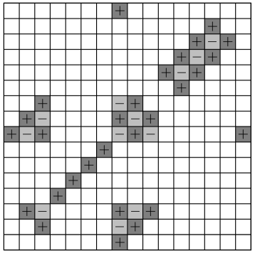

The corresponding (nonempty) sets and , where and , are depicted on Figure 1 right, along with the values for on top (note that ). In particular,
Next, we give some basic properties of the sets defined above.
Lemma 4.
For all we have
Proof.
We prove this by induction on . From equations (2) and (4) if follows that , so the claim holds for . Suppose it holds for some and let . Then, by equation (5), either or . In the first case . In the second case for some . Since and is a union of some subfamily of , it follows that , because is a refinement of for any . By equation (2) we conclude that , which finishes the proof. ∎
Lemma 5.
For any the sets with are disjoint.
Proof.
If , then , while is a union of some subfamily of . Hence, either or . So if and , then . By equation (5) this implies that the sets and are disjoint. The claim now follows. ∎
Lemma 5 implies that for every we have a disjoint (double) union
| (6) |
Next lemma shows that the sequence of sets is decreasing in with respect to inclusion.
Lemma 6.
for all .
3.2. Measure-theoretic properties of sets and
Note that all subsets of considered above are open, so they are Borel measurable. We will now show that the Lebesgue measure of is small.
Lemma 7.
for all .
Proof.
We can now give one of the key points of this construction. Let
| (7) |
The first crucial property of the set is that its Lebesgue measure is .
Lemma 8.
We have .
Proof.
Furthermore, the restriction of measure to the set is the zero measure.
Lemma 9.
The measures defined for all by
is the zero measure.
Proof.
Let be arbitrary and let . Then
Taking into account the monotonicity of , see Lemma 6, and the fact that is a finite signed measure, we obtain
Using equation (6) and the fact that the union in (6) is disjoint by Lemma 5, we obtain
| (8) | ||||
For any rectangle , where stands for either or , the continuity, groundedness and -Lipschitz property of quasi-copulas imply
regardless of whether is empty or not. Applying this inequality to the rectangle in (8) and using also Lemma 8 we obtain
and consequently . To prove that is the zero measure on we use a standard argument. By the above the collection is a -algebra that contains all rectangles of the form . Hence, and is the zero measure. ∎
As a consequence to Lemma 9, we obtain the second crucial property of the set , which will be essential for the convergence of measures constructed later.
Lemma 10.
We have
Proof.
By Lemma 9, the measure defined in that lemma is a zero measure. Denote the support of by . Then
and similarly . The claim now follows since .
∎
Switching the first and second coordinate in the above constructions, we can analogously define for all and the sets
| (9) |
By symmetry the versions of Lemmas 7–10 for the sets and also hold. In particular, for all , , the measure defined for all by
is the zero measure, and the following lemma holds.
Lemma 11.
We have
3.3. Construction of quasi-copulas
We now turn our attention to the construction of a sequence of quasi-copulas . For every positive integer denote the complements
By equations (6) and (9) the sets and are open, so the sets and are closed and contain and . The restriction of quasi-copula to the set is a sub-quasi-copula according to [22, Definition 2.3]. We can extend sub-quasi-copula to a quasi-copula using the formula from the proof of [22, Theorem 2.3], which we recall now. Let be an arbitrary point in and denote
Then and . If , then , and if , then . Now let
Then the value of the extension at is given by
| (10) | ||||
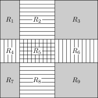
Note that is bilinear on . In particular, if is a closed rectangle such that only the vertices of lie in , then is bilinear on (e.g. on Figure 2). If only the left and right side of lie in , then is linear in on but not necessary in (e.g. and on Figure 2), if only the bottom and top side of lie in , then is linear in on but not necessary in (e.g. and on Figure 2), and if the whole lies in , then on is not linear in any coordinate in general (e.g. , , , and on Figure 2). So the extension is as linear as possible. This means that it spreads mass on uniformly in certain directions, which will be important later on.
3.4. Construction of measures
We aim to prove that quasi-copulas induce signed measures on . We now construct these measures. From equations (6) and (9) it follows that the sets and are countable unions of disjoint open intervals, say
| (11) |
where each and is a member of . We are assuming here without loss of generality that the unions are infinite. If they are finite the arguments are essentially the same.
For a set with , define a probability measure on by
for all , and finite signed measures and on by
| (12) |
for all . Furthermore, introduce finite signed measures and on by
| (13) | ||||
and
| (14) |
for all , where denotes both the product of measures and the Cartesian product of sets. The idea behind the definition of is that it should correspond to the measure induced by the the extension on the set . In particular, the first sum corresponds to the regions where is linear in the coordinate (regions and on Figure 2), the second sum corresponds to the regions where is linear in coordinate (regions and on Figure 2) and the third sum corresponds to the regions where is bilinear (region on Figure 2).
We first need to show that is well defined.
Lemma 12.
For every the sum in equation (13) converges in the total variation norm, so is a finite signed measure on .
Proof.
For every with let be the Jordan decomposition of and denote the supports of and by and , respectively. Since is a probability measure, and and are positive measures, we can estimate using equation (1)
| (15) | ||||
Using equations (1) and (12) we estimate
| (16) | ||||
Combining inequalities (15) and (16) gives
and similarly we obtain
These two inequalities imply
| (17) | ||||
Since the vector space of all finite measures equipped with the total variation norm is a Banach space, this implies that the sum in equation (13) converges in the total variation norm and is a finite signed measure. ∎
We can now prove that quasi-copulas induce signed measures. For every define a finite signed measure
where and are given in equations (13) and (14). We show with a direct calculation that measure is induced by .
Lemma 13.
For every quasi-copula induces signed measure .
Proof.
We consider four cases, depending on where the point lies.
Case 1: and . On Figure 2 this corresponds to . In this case is not contained in any and is not contained in any so equation (18) becomes
Since
and this union is disjoint, we conclude
| (19) |
By equation (10) this is equal to because and .
Case 2: and . On Figure 2 this corresponds to . We may assume without loss of generality that since the order of the intervals in equation (11) is arbitrary. On the other hand, is not contained in any . By splitting , we infer that equation (18) can be written as
Note that , so we may use Case 1 to evaluate the first term in the above expression. Using equation (19), the first term is equal to . Furthermore, the last term and the first of the two sums are equal to because . Hence,
| (20) | ||||
Finally, by continuity of we can express
By equation (10) this is equal to because and .
Case 3: and . On Figure 2 this corresponds to . This case is treated similarly as Case 2. Assuming , we obtain
which is again equal to by equation (10).
Case 4: and . On Figure 2 this corresponds to . We may assume without loss of generality that and . By splitting , we infer that equation (18) can be written as
Note that , so by Case 2, using equation (20), the first term in the above expression is equal to
Furthermore, the last term and the first of the two sums are equal to because . Hence,
We can simplify the last sum, also using , to obtain
| (21) | ||||
Note that
so we may combine the second and third row of equation (21) to get
The continuity of implies
so that
By equation (10) this is again equal to because and . ∎
Next step is to establish the convergence of finite signed measures .
Lemma 14.
The sequence of measures converges to in the total variation norm.
Proof.
From the proof of Lemma 12, see in particular inequality (17), it follows that
When tends to infinity, the right-hand side converges to by Lemmas 10 and 11, so the sequence of measures converges to the zero measure in the total variation norm. Furthermore, note that
for all . So we can use equation (1) and an analogous calculation as in inequality (16) to obtain
Using a similar argument as for , we infer that the sequence converges to the zero measure, so that converges to in the total variation norm. We conclude that the sequence of finite measures converges to . ∎
3.5. Decomposition of quasi-copulas
We have so far shown that quasi-copulas induce signed measures and the measures converge in the total variation norm to measure , which is induced by .
The final property of quasi-copulas that we need is that every is a linear combination of two copulas. To prove this we will show that each satisfies condition of Theorem 2.
Lemma 15.
For every there exist bivariate copulas and and real numbers and such that . Consequently, .
Proof.
Fix . By Theorem 2 it suffices to prove that
where for all and for all . Let and . The continuity of implies
therefore
| (22) |
Equation implies for all . Similarly, for all . Hence, by equations (13) and (14),
where we also used . This implies
From equations (12) and (14) we infer
therefore
| (23) | ||||
We now consider two cases.
Case 1: . Note that but because . Hence, by equation (6). This implies that there exists with and such that intersects . But then because and . By equation (11) we may assume without loss of generality that . Hence, does not intersect any with . It now follows from inequality (23) and from that
or equivalently
Since with and the set is disjoint from , Lemma 4 and equation (2) imply that . By condition (3) we have , hence
| (24) |
Case 2: . Note that each is a member of . Hence, we have three options for each , namely, the interval does not intersect , the interval is contained in , or the interval contains . By the case assumption and equation (11), option cannot happen, so the interval contains all that it intersects. In particular,
Thus, inequality (23) implies
| (25) | ||||
Furthermore, , otherwise Lemma 4 and equation (6) would imply that . By condition (3) this implies
This, together with inequality (25), gives
| (26) |
Combining inequalities (24) and (26) with inequality (22) gives
Since and were arbitrary, we infer
By symmetry we also obtain
Consequently, , as required. ∎
Let us summarize the results of this section that we will need for the proof of Theorem 1.
Theorem 16.
Let be a bivariate quasi-copula that induces a signed measure on . Then there exists a sequence of bivariate quasi-copulas , , such that
-
for some bivariate copulas and and some real numbers and , and
-
the sequence of induced measures converges to in the total variation norm.
4. Proof of the main theorem
In this section we continue assuming that is a bivariate quasi-copula that induces a signed measure . By Theorem 16 we obtain a sequence of measures , induced by quasi-copulas , that converges to in the total variation norm. We will now convert the sequence of measures into a series, which will be manipulated to produce a converging series of multiples of measures induced by copulas. We will employ a method that was used in [7] for converting a sequence of quasi-copulas into a function series converging in the supremum norm. We just need to apply the method to a sequence of measures converging in the total variation norm.
First we construct the series
| (27) |
Partial sums of this series are measures , so by Theorem 16 the series converges in the total variation norm and its sum is . Theorem 16 also implies that for some bivariate copulas and and some real numbers and . Note that . If both and are positive, is a convex combination of copulas, so it is a copula itself and we may assume , , and . If at least one of and is negative, we may assume , and consequently . So we have and for all . Furthermore,
for all , where and . Since and for all , the functions
| (28) |
for all are convex combinations of copulas, so they are copulas themselves. Denote also
| (29) |
for all so that
In addition, let
| (30) |
Then the series in equation (27) is expressed as
| (31) |
If we omit the parenthesis in series (31), the resulting series
is not convergent in the total variation norm. For example, evaluating it on the set we obtain the series , which is divergent, in fact, oscillating, since and . Before we omit the parenthesis in series (31), we need to split its terms into sums of terms with small enough norm, so that after omitting the parenthesis the ”oscillation” will tend to . For every we choose a positive integer . We rewrite the series in equation (31) as
| (32) |
and remove the parenthesis to obtain the series
| (33) | ||||
We now prove the following.
Lemma 17.
The series of finite signed measures (33) converges to in the total variation norm.
Proof.
The difference between and any partial sum of series (33), is of the form
for some , , and . We can estimate its total variation norm as follows
Using and the fact that is a probability measure, we obtain
When tends to infinity, the first term converges to , the second term converges to because it is the norm of a single term of a converging series (31), and the last term converges to because it is the norm of the tail of a converging series (31). This proves that the partial sums of series (33) converge to in the total variation norm. ∎
We are now finally ready to prove Theorem 1.
Proof of Theorem 1.
: Assume that a quasi-copula induces a signed measure on . Let be the sequence of copulas
defined in equations (28) and (30), and let be the sequence of real numbers
defined in equations (29) and (30). By Lemma 17 the series converges in the total variation norm to , which proves condition . For all and we have
Hence, the convergence of the series in the total variation norm implies that the series converges uniformly to . This proves condition .
: By condition the sum of the series is a finite signed measure on . Denote this measure by . As above, this implies that the series converges uniformly to the function . On the other hand, this series converges to by condition . Hence, for all . ∎
We note that if condition of Theorem 1 holds, then the series in condition converges to . This implies that a measure induced by a bivariate quasi-copula can always be expressed as a converging sum of multiples of measures induced by bivariate copulas, i.e., as what we can call an infinite linear combination of measures induced by copulas.
Corollary 18.
Any measure induced by some measure-inducing bivariate quasi-copula can be expressed as where each is a measure induced by some bivariate copula, each is a real number, and the series converges in the total variation norm.
As another corollary to Theorem 1 we obtain the following interesting property.
Theorem 19.
Let be a bivariate quasi-copula that induces a signed measure on . Then
| (34) |
is a joint distribution function of two absolutely continuous random variables and with ranges in .
Proof.
Let and be the sequences from Theorem 1, so that . Function is clearly a distribution function of two random variables and with support in . The cumulative distribution of is given by
Let be the positive measure induced by , i.e., for all . Suppose satisfies . Let and be the supports of measures and , respectively. Then
Since is a positive measure, and similarly for all . Hence, . This shows that measure is absolutely continuous with respect to Lebesgue measure. By Radon-Nikodym theorem there exists a -measurable function such that . Therefore, is absolutely continuous random variable with density . Similarly, is also absolutely continuous. ∎
5. Example
We conclude this paper with an example illustrating Theorem 1 and Corollary 18. In [7, Example 13] the authors construct an example of a quasi-copula , that induces a finite signed measure, but cannot be written as a linear combination of two copulas. This implies that its induced measure cannot be written as a linear combination of two measures induced by copulas. On the other hand, by Corollary 18, measure can be expressed as an infinite linear combination of measures induced by copulas. We now find such a representation of .
First, we briefly recall the definition of quasi-copula , for some additional details see [7, Example 13]. For a positive integer let be a discrete quasi-copula defined on an equidistant mesh , which has mass distributed in a checkerboard pattern (of positive and negative values) within the central diamond-shaped area (with no mass outside this area), so that there are exactly squares with positive mass and squares with negative mass . For example, the spread of mass of is given by the matrix
If we denote by the bilinear extension of to , then quasi-copula is defined as an ordinal sum of quasi-copulas , with respect to the partition , where and . Since the length of is , the summand contributes a total mass of to the mass of .
Denote the product copula by . Note that for every positive integer the function is clearly grounded and has uniform marginals. In fact, it is a copula since its mass is nowhere negative and its total mass is equal to . We can express
| (35) |
For a positive integer denote by the ordinal sum with respect to partition , where the -th summand is and all other summands are . In addition, denote by the ordinal sum with respect to partition , where all the summands are .
We claim that
| (36) |
Indeed, the series on the right converges in the total variation norm because the support of measure is contained in , so by equation (35)
and the series is convergent with sum . In addition, on each the sum of the series in (36) coincides with by equation (35), because only the two terms and are nonzero there. This implies that the sum of the series in (36) is indeed equal to .
Acknowledgments
The author would like to thank Damjana Kokol Bukovšek for useful discussions and comments that helped to improve the presentation of this paper. The author acknowledges financial support from the ARIS (Slovenian Research and Innovation Agency), research core funding No. P1-0222.
References
- [1] C. Alsina, R. B. Nelsen, and B. Schweizer, On the characterization of a class of binary operations on distribution functions, Statist. Probab. Lett. 17 (1993), no. 2, 85–89. MR 1223530
- [2] J. J. Arias-García and B. De Baets, On the lattice structure of the set of supermodular quasi-copulas, Fuzzy Sets and Systems 354 (2019), 74–83. MR 3906655
- [3] J. J. Arias-García, R. Mesiar, and B. De Baets, A hitchhiker’s guide to quasi-copulas, Fuzzy Sets and Systems 393 (2020), 1–28. MR 4102063
- [4] N. A. Buliah and W. L. S. Yie, Modelling of extreme rainfall using copula, AIP Conference Proceedings 2266 (2020), 090007.
- [5] B. De Baets, H. De Meyer, and M. Úbeda Flores, Extremes of the mass distribution associated with a trivariate quasi-copula, C. R. Math. Acad. Sci. Paris 344 (2007), no. 9, 587–590. MR 2323747
- [6] M. Dibala, S. Saminger-Platz, R. Mesiar, and E. P. Klement, Defects and transformations of quasi-copulas, Kybernetika (Prague) 52 (2016), no. 6, 848–865. MR 3607851
- [7] G. Dolinar, B. Kuzma, and N. Stopar, Quasi-copulas as linear combinations of copulas, Fuzzy Sets and Systems 477 (2024), Paper No. 108821, 15. MR 4677117
- [8] F. Durante, J. Fernández-Sánchez, and W. Trutschnig, Baire category results for quasi-copulas, Depend. Model. 4 (2016), no. 1, 215–223. MR 3555169
- [9] F. Durante, J. Fernández-Sánchez, W. Trutschnig, and M. Úbeda Flores, On the size of subclasses of quasi-copulas and their Dedekind–MacNeille completion, Mathematics 8 (2020), no. 12, 2238.
- [10] N. C. Dzupire, P. Ngare, and L. Odongo, A copula based bi-variate model for temperature and rainfall processes, Scientific African 8 (2020), e00365.
- [11] J. Fernández-Sánchez, R. B. Nelsen, and M. Úbeda Flores, Multivariate copulas, quasi-copulas and lattices, Statist. Probab. Lett. 81 (2011), no. 9, 1365–1369. MR 2811851
- [12] J. Fernández-Sánchez, J. A. Rodríguez-Lallena, and M. Úbeda Flores, Bivariate quasi-copulas and doubly stochastic signed measures, Fuzzy Sets and Systems 168 (2011), 81–88. MR 2772622
- [13] A. J. McNeil, R. Frey, and P. Embrechts, Quantitative risk management, revised ed., Princeton Series in Finance, Princeton University Press, Princeton, NJ, 2015, Concepts, techniques and tools. MR 3445371
- [14] R. B. Nelsen, An introduction to copulas, second ed., Springer Series in Statistics, Springer, New York, 2006. MR 2197664
- [15] R. B. Nelsen, J. J. Quesada-Molina, J. A. Rodríguez-Lallena, and M. Úbeda Flores, Some new properties of quasi-copulas, Distributions with given marginals and statistical modelling, Kluwer Acad. Publ., Dordrecht, 2002, pp. 187–194. MR 2058992
- [16] by same author, Quasi-copulas and signed measures, Fuzzy Sets and Systems 161 (2010), no. 17, 2328–2336. MR 2658036
- [17] R. B. Nelsen and M. Úbeda Flores, The lattice-theoretic structure of sets of bivariate copulas and quasi-copulas, C. R. Math. Acad. Sci. Paris 341 (2005), no. 9, 583–586. MR 2182439
- [18] M. Omladič and N. Stopar, Final solution to the problem of relating a true copula to an imprecise copula, Fuzzy Sets and Systems 393 (2020), 96–112. MR 4102064
- [19] by same author, Dedekind-MacNeille completion of multivariate copulas via ALGEN method, Fuzzy Sets and Systems 441 (2022), 321–334. MR 4434854
- [20] by same author, Multivariate imprecise Sklar type theorems, Fuzzy Sets and Systems 428 (2022), 80–101. MR 4347444
- [21] A. Onken, S. Grünewälder, M. H. J. Munk, and K. Obermayer, Analyzing short-term noise dependencies of spike-counts in Macaque prefrontal cortex using copulas and the flashlight transformation, PLoS Comput. Biol. 5 (2009), no. 11, e1000577, 13. MR 2577405
- [22] J. J. Quesada Molina and C. Sempi, Discrete quasi-copulas, Insurance Math. Econom. 37 (2005), no. 1, 27–41. MR 2156594
- [23] C. Sempi, A study of the mass distribution of quasi-copulas, Fuzzy Sets and Systems 466 (2023), Paper No. 108467, 5. MR 4594098
- [24] M. Úbeda Flores, Extreme values of the mass distribution associated with a tetravariate quasi-copula, Fuzzy Sets and Systems 473 (2023), Paper No. 108728, 5. MR 4649324