Efficient Learning Using Spiking Neural Networks Equipped With Affine Encoders and Decoders

Abstract

We study the learning problem associated with spiking neural networks. Specifically, we consider hypothesis sets of spiking neural networks with affine temporal encoders and decoders and simple spiking neurons having only positive synaptic weights. We demonstrate that the positivity of the weights continues to enable a wide range of expressivity results, including rate-optimal approximation of smooth functions or approximation without the curse of dimensionality. Moreover, positive-weight spiking neural networks are shown to depend continuously on their parameters which facilitates classical covering number-based generalization statements. Finally, we observe that from a generalization perspective, contrary to feedforward neural networks or previous results for general spiking neural networks, the depth has little to no adverse effect on the generalization capabilities.

1 Introduction

Deep learning [29, 6] is a technology that has revolutionized many areas of modern life. The term describes the gradient-based training of deep neural networks. Since its breakthrough in image classification in 2012 [28], deep learning is essentially the only viable technology for this application. Moreover, it is the basis of multiple recent breakthroughs in science [25] and even mathematical research [14]. Recently, deep learning has received wide public attention through the advent of generative AI in the form of large language models such as ChatGPT [39].

It is well-documented that deep learning in modern applications can have extreme requirements on computational resources and the hardware requirements scale in an unsustainable way [52]. In constrained settings, this can become a serious bottleneck preventing the employment of deep learning methods. In addition, these comprehensive computations come with an immense environmental cost.

As a consequence, to develop more powerful tools, the computational cost needs to be controlled. Neuromorphic computing offers one potential solution to this problem. This computation paradigm is based on employing so-called spiking neural networks (SNNs) [32], which are more closely related to biological neural networks, and significantly more energy efficient than deep neural networks. Mathematically, it can be rigorously shown that SNNs can represent certain functions, such as coincidence detectors, with much fewer parameters than feedforward neural networks [1].

In this work, we will contribute to the understanding of improved efficiency by studying approximation and learning problems associated with SNNs.

We study the so-called simple spike model [36] in the formalism introduced in [49] and find that the associated set of SNNs differs in a crucial and fundamental way from sets of feedforward neural networks. The difference lies in the fact that these sets of SNNs are not continuously parameterized by their parameter set. We will expand on this issue in the next subsection.

To overcome said discontinuity, we introduce a modification to the traditional definition of SNNs, which we coin affine SNNs. Affine SNNs distinguish themselves through two properties. First, only positive weights are allowed. Second, we allow the output and the input of these SNNs to be composed with affine maps. This corresponds to the choice of appropriate temporal encoders and decoders in [49].

Despite the restriction on the weights, affine SNNs can reproduce many approximation results by feedforward neural networks, such as the approximation of smooth functions at optimal rates or dimension-independent rates for Barron functions. Moreover, when using empirical risk minimization to find affine SNNs solving a learning problem, the generalization gap can be controlled linearly up to a log factor by the number of parameters involved. Notably, we find that unlike for feedforward neural networks (or previous VC dimension-based analyses of SNNs [45, 36]), our generalization bounds depend at most logarithmically on a notion of depth for SNNs. Therefore, affine SNNs are a novel computational paradigm that combines advantageous properties of feedforward neural networks with superior generalization performance and more energy-efficient implementability.

1.1 Spiking neural networks and continuous parameterizations

To describe our work in more detail, we introduce a very limited definition of an SNN that will be refined later. Indeed, we only require spiking neurons in this introduction. For the purposes of this introduction, a spiking neuron is a function of input times $t_{1},\dots,t_{n}\in\mathbb{R}$, for $n\in\mathbb{N}$, that outputs the smallest number $t^{\star}\in\mathbb{R}$ such that $\sum_{i=1}^{n}w_{i}\varrho(t^{\star}-t_{i}-d_{i})=1$, where $\varrho(x)\coloneqq\max\{0,x\}$ denotes the ReLU activation function, $(w_{i})_{i=1}^{n}\in\mathbb{R}^{n}$ is a vector of weights, and $(d_{i})_{i=1}^{n}\in\mathbb{R}^{n}$ is a vector of delays.

Consider the following example of three-dimensional inputs. Let $s\in\mathbb{R}$. Let $w_{1}=1,w_{2}=-1,w_{3}=1$ and $d_{1}=0$, $d_{2}=1+s$, $d_{3}=2$, and we call the associated spiking neuron $\nu_{s}$. It is not hard to see that for every $t\in\mathbb{R}$

$$\nu_{s}(t,t,t)=\left\{\begin{array}[]{ll}t+2-s&\text{ if }s<0\\ t+1&\text{ if }s\geq 0.\end{array}\right.$$

We observe that $\|\nu_{s}-\nu_{-s}\|_{L^{\infty}}\geq 1$ for all $s\in\mathbb{R}$. Letting $s\to 0$ demonstrates that $\nu_{s}$ does not depend continuously on its parameters.

Since the parameterization is not continuous, we conclude that optimizing the parameters to minimize an objective of the output of a spiking neuron is a discontinuous problem. Hence, contrary to the training of feedforward neural networks, gradient-based training is not well-defined for SNNs.

1.2 Our contribution

In this paper, we identify the fact that the weights in SNNs are allowed to be negative or arbitrarily close to zero as a reason why the parameterization of SNNs through their weights is not continuous.

We propose a solution to this shortcoming via a modified type of SNNs called affine SNNs. Affine SNNs have positive weights only, and it will be demonstrated in Theorem 3.6 that affine SNNs depend continuously on their parameters.

Despite the restriction on their weights, affine SNNs are still remarkably powerful. We collect the results in Section 5. There we find the following:

1. Affine SNNs are universal approximators, i.e., every continuous function on a compact domain can be arbitrarily well approximated by an affine SNN, Theorem 5.4;

2. Affine SNNs can replicate approximation results achieved by linear finite elements, Theorem 5.7. In particular, they approximate, at optimal approximation rates, Sobolev-regular smooth functions, Theorem 5.9.

3. Affine SNNs can produce dimension-independent approximation rates for Barron-regular functions, Theorem 5.11.

All of these approximation results are shared with feedforward neural networks [13, 21, 4]. It is known that the approximation of elements from a finite element space is impossible with shallow feedforward neural networks [21].

Moreover, for an input dimension $d$, the specific construction in [21] has depth $\log(d)$, but it needs to be added that this depth scaling with the input dimension is not necessary, as a depth of $\mathcal{O}(\log(\log(d))$ was shown to suffice in [43, Theorem 3.2]. At the moment, we are not aware of a construction where the depth can be chosen independent of the dimension if the width should be chosen in $\mathcal{O}(d)$. In contrast to the situation for feedforward neural networks, our construction based on SNNs requires just two compositions (in the sense of spiking neurons being applied to the outputs of other spiking neurons), which would correspond to a feedforward neural network with two hidden layers.

We will complement our analysis by studying the learnability of affine SNNs. Surprisingly, we will find that, to keep the generalization gap under control, we need a number of training samples that only depend linearly on the number of parameters (and their magnitude), Theorem 4.3. In particular, the required number of samples depends at most logarithmically on the depth of the SNNs. Note that this is in contrast to previous results for the VC dimension of deep (non-affine, real weights) SNNs, which scales linearly with the depth [45].

In Section 6, we combine the generalization and approximation results to obtain full error bounds for the empirical risk minimization problem for target functions from the classes for which we have derived expressivity statements.

Overall, we observe the following remarkable property of affine SNNs: The capacity cost for learning, i.e., the complexity of the hypothesis set, is bounded with at most logarithmic dependence on the depth of the underlying affine SNNs. Hence, SNNs can solve problems that shallow feedforward neural networks cannot solve at practically no higher capacity cost than shallow neural networks.

In conclusion, we believe that the construction presented in this work is a first step toward identifying SNN constructions that admit

1. continuously dependence on parameters,

2. no worse approximation performance than deep feedforward neural networks for relevant function classes,

3. better performance than deep feedforward neural networks in some tasks,

4. superior generalization performance over deep feedforward neural networks.

However, we note that our construction does not yet fully achieve this desired program because we have not found an approximation result of affine SNNs that reproduces approximation results by deep neural networks, such as given in [51, 53].

1.3 Related work

The research on SNNs is vast and has been developed over multiple decades. For a more comprehensive overview, we refer to the survey articles [32, 41, 20]. In the following, we will focus on the literature that is most closely related to the expressivity and learning problems discussed in this paper.

SNNs come in multiple types that differ in the way of encoding and decoding the input signals. These types include rate encoding, density encoding, and temporal encoding [35, 18]. Moreover, different models of spiking neurons exist, such as the Hodgkin–Huxley model [22, 23], the integrate-and-fire model [50], or the spike response model [16, 27]. This work deals with the spike response model with temporally encoded inputs. In this framework, the expressivity of SNNs has been studied extensively, e.g., [31, 32, 34, 49]. This includes the universal approximation property [11] as well as other, more quantitative approximation rates [49, Section 3.3].

Our results distinguish themselves from previous works due to our requirement of positive weights, which offers significantly less flexibility.

Concerning learning rates, it was shown in [36, 37, 45] that classical statistical learning theory bounds can be derived. These are in terms of the VC dimension or the pseudo-dimension. In contrast, our results will use covering number estimates and yield stronger generalization guarantees since the upper bounds will only depend logarithmically on the depth of the SNNs.

1.4 Feedforward neural networks

A comprehensive overview of the relevant literature on feedforward neural network-based learning is given in [8].

The approximation theory of feedforward neural networks is comparatively very well understood. First of all, universality properties have been shown for various architectures [13, 24, 26]. Moreover, for specific function classes approximation rates can be derived. For example, focusing only on feedforward neural networks with the ReLU activation function, it was established that neural networks can reproduce approximation by linear and higher order finite elements [21, 40], achieve optimal approximation of smooth functions [53, 47], and approximate high-dimensional functions without curse of dimensionality [4].

Regarding learning guarantees, classical statistical learning theory facilitates generalization through, for example, VC dimension, covering number or pseudo-dimension bounds [46, 8, 2]. Applied specifically to ReLU neural networks, such generalization bounds are, for example, derived in [7, 44].

It has to be mentioned that in the context of modern machine learning applications using overparameterized architectures, classical statistical learning theory-based arguments are potentially void, and different tools are required [54, 5].

2 Notions of spiking neural networks

In this section, we introduce the central concepts of this paper. Specifically, we will describe the SNN architectures and the concept of firing times. SNNs are based on the so-called network graphs introduced below.

Definition 2.1.

A (finite) directed, unweighted graph $G=(V,E)$ satisfying the following properties:

1. $G$ has no directed cycles,

2. $G$ has no isolated nodes,

is called a directed acyclic graph or a network graph. We denote the set of all nodes with no incoming edges as $V_{\rm in}$, referred to as the input nodes, and the set of nodes with no outgoing edges as $V_{\rm out}$, referred to as the output nodes. We refer to the length of the longest directed path in $G$ as the (graph) depth of $G$.

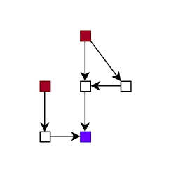
Figure 1: A network graph $G$ with two input nodes in burgundy and one output node in violet

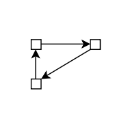
Figure 2: An example of a forbidden directed cycle

Figures 2, 2 provide an example and a non-example of a network graph, respectively.

Based on a network graph, various definitions of SNNs are possible. In Subsection 2.1, we specify our model of SNNs, and in Subsection 2.2, we draw comparisons between our setups and others documented in the literature. Following this, in Subsection 2.3, we introduce affine SNNs. Finally, in Subsection 2.4, we present a useful operation applicable to affine SNNs, facilitating the construction of more complex networks.

In this paper, we denote the cardinality of a set $S$ by $\#S$. Drawing inspiration from graph theory, neural networks, and biology, we will also use the terms “node”, “vertex” and “neuron” interchangeably.

2.1 Spiking neural network model

We now present the definition of a general SNN as an architecture, followed by a description of its dynamics. Afterward, we proceed to introduce a special type of positive SNNs.

Definition 2.2.

Let $G=(V,E)$ be a network graph with a subset $V_{\rm in}\subset V$ of input neurons, a subset $V_{\rm out}\subset V$ of output neurons, and a set $E\subset V\times V$ of synapses. Each synapse $(u,v)\in E$ is a directed edge, associated with the following attributes

1. a response function $\varepsilon_{(u,v)}\colon\mathbb{R}\to\mathbb{R}$,

2. a synaptic delay $d_{(u,v)}\geq 0$,

3. a synaptic weight $\mathsf{w}_{(u,v)}\geq 0$.

Moreover, for every $v\in V\setminus V_{\rm in}$, there exists $(u,v)\in E$ such that $\mathsf{w}_{(u,v)}>0$.

Lastly, let $\mathsf{W}\coloneqq(\mathsf{w}_{(u,v)})_{(u,v)\in E}$, $D\coloneqq(d_{(u,v)})_{(u,v)\in E}$, and $\mathcal{E}\coloneqq(\varepsilon_{(u,v)})_{(u,v)\in E}$ be the tuple of synaptic weights, synaptic delays, and response functions, respectively. Then a spiking neural network (SNN) is a tuple $\Phi=(G,\mathsf{W},D,\mathcal{E})$.

In the sequel, we will focus on SNNs for which the response function is the same for all edges. Concretely, inspired by [49], we adopt a unified response function modeled after the ReLU activation function.

Definition 2.3.

Let $G$ be a network graph, and let $(u,v)$ be one of its synapses. We define the response function $\varepsilon_{(u,v)}:\mathbb{R}\to\mathbb{R}$ associated with $(u,v)$ as follows

$$\varepsilon_{(u,v)}(t)\coloneqq\varrho(t)$$ (2.1)

where $\varrho(t)=\max\{t,0\}$ denotes the ReLU activation function.

Information is propagated through an SNN by the neuron firings. This process is determined through so-called firing times that are initiated by a so-called membrane potential, or simply potential, reaching a critical value. We state the mathematical model below.

Definition 2.4.

Let $\Phi=(G,\mathsf{W},D,\mathcal{E})$ be an SNN, and let $G=(V,E)$ be a network graph. Let $\varepsilon_{(u,v)}\in\mathcal{E}$ be defined as in (2.1). Let $t_{u}\in\mathbb{R}$ for $u\in V_{\rm in}$. Then, for $v\in V\setminus V_{\rm in}$, we define the potential at $v$ as $P_{v}\colon\mathbb{R}\to\mathbb{R}$, where for $t\in\mathbb{R}$

$$P_{v}(t)\coloneqq\sum_{(u,v)\in E}\mathsf{w}_{(u,v)}\varepsilon_{(u,v)}(t-t_{u}-d_{(u,v)})=\sum_{(u,v)\in E}\mathsf{w}_{(u,v)}\varrho(t-t_{u}-d_{(u,v)}).$$ (2.2)

Here in (2.2), $t_{u}=\min\{t\in\mathbb{R}\colon P_{u}(t)=1\}$ is the firing time at $u$ if $u\in V\setminus V_{\rm in}$. Subsequently, the firing time $t_{v}$ at $v$ is given by $t_{v}=\min\{t\in\mathbb{R}\colon P_{v}(t)=1\}$.

A few remarks are in order. First, the provided definition may appear circular, as the firing time at a noninput neuron is determined by its potential, which, in turn, hinges on the firing times of other presynaptic neurons. Second, it does not inherently guarantee that $\min\{t\in\mathbb{R}\colon P_{u}(t)=1\}$ is nonempty.

The following lemma demonstrates the well-definedness of $P_{v}$ and $t_{v}$ for all $v\in V\setminus V_{\rm in}$, when the responses $\varepsilon_{(u,v)}$ are of the form (2.1). A proof is given in Appendix A.1.

Lemma 2.5.

Let $\Phi=(G,\mathsf{W},D,\mathcal{E})$ be an SNN where $G=(V,E)$ is a network graph. Let $\varepsilon_{(u,v)}\in\mathcal{E}$ be defined as in (2.1). Let $t_{u}\in\mathbb{R}$ for $u\in V_{\rm in}$. Then $P_{v}$ and $t_{v}$ are well-defined for all $v\in V\setminus V_{\rm in}$.

We conclude this subsection by formalizing the selected SNNs for this work, referred to as positive SNNs.

Definition 2.6.

Let $\Phi=(G,\mathsf{W},D,\mathcal{E})$ be an SNN with $G=(V,E)$ being a network graph. Then $\Phi$ is a positive SNN if for all $(u,v)\in E$, $\mathsf{w}_{(u,v)}>0$, and $\varepsilon_{(u,v)}$ is given by (2.1). Moreover, if $\Phi$ is a positive SNN, we streamline its tuple notation as $\Phi=(G,\mathsf{W},D)$.

Since Lemma 2.5 asserts in particular that $t_{v}$ exists for $v\in V_{\rm out}$ once $t_{u}$ is assigned for all $u\in V_{\rm in}$ in a positive SNN $\Phi$, we can define a map taking all input firing times to the output firing times. This function is called the realization of $\Phi$.

Definition 2.7.

Let $\Phi=(G,\mathsf{W},D)$ be a positive SNN. Let ${\rm d}_{\rm in}$, ${\rm d}_{\rm out}$ denote the cardinality of $V_{\rm in}$, $V_{\rm out}$, respectively. Then the realization of $\Phi$, $\mathsf{R}(\Phi):\mathbb{R}^{{\rm d}_{\rm in}}\to\mathbb{R}^{{\rm d}_{\rm out}}$, is a function whose inputs are $(t_{v})_{v\in V_{\rm in}}\in\mathbb{R}^{{\rm d}_{\rm in}}$ and whose outputs are $(t_{v})_{v\in V_{\rm out}}\in\mathbb{R}^{{\rm d}_{\rm out}}$, where $t_{v}$ denotes the firing time at neuron $v$.

It is to be understood from the definition above and throughout this paper that we assume a consistent enumeration of the input and output neurons.

2.2 Comparison with existing literature

In this subsection, we offer an interpretation of our architectures and describe their significance. Concurrently, we draw comparisons with related works to place our model of SNNs within the existing literature on SNNs. To begin, it is worth recalling that, as per Definition 2.2, the architecture of an SNN $\Phi=(G,\mathsf{W},D,\mathcal{E})$, given a network graph $G=(V,E)$, is established once the synaptic weights $\mathsf{W}=(\mathsf{w}_{(u,v)})_{(u,v)\in E}$, the synaptic delays $D=(d_{(u,v)})_{(u,v)\in E}$, and the response functions $\mathcal{E}=(\varepsilon_{(u,v)})_{(u,v)\in E}$ are determined. In our model of positive SNNs $\Phi=(G,\mathsf{W},D)$, Definition 2.6, we require the synaptic weights to be positive and the response functions to be of the form (2.1). We discuss these two requirements further below.

Enforcing positive synaptic weights implies that an edge $(u,v)$ is present if and only if $\mathsf{w}_{(u,v)}>0$. The rationale behind this is straightforward. As evident from Definition 2.2, a neuron $u$ can transmit a signal to a neuron $v$ if and only if there exists an edge $(u,v)\in E$ with $\mathsf{w}_{(u,v)}>0$. Therefore, synaptic weights describe the strength of neural connections, which, combined with the assigned responses, impact the firing times. Consequently, when an edge $(u,v)$ has $\mathsf{w}_{(u,v)}=0$, it effectively suppresses the charge contribution from $u$ to $v$ and has the same effect as removing the edge $(u,v)$ from the network.

To justify the choice of the response mechanism (2.1), we first need to recall the following response function cited in [49],

$$\tilde{\varepsilon}_{(u,v)}(t)\coloneqq\begin{cases}0&\text{ if }t\not\in[d_{(u,v)},d_{(u,v)}+\delta]\\ s_{(u,v)}\varrho(t-d_{(u,v)})&\text{ if }t\in[d_{(u,v)},d_{(u,v)}+\delta]\end{cases},$$ (2.3)

for $t\in\mathbb{R}$. Here, $\delta\in(0,\infty]$ is given, and $s_{(u,v)}=\pm 1$ depending on the synapse $(u,v)$. When $s_{(u,v)}=1$, the response at neuron $v$ stimulated by the firing from neuron $u$ corresponds to a biological excitatory synapse. Moreover, if $\delta=\infty$, we recover (2.1). When $s_{(u,v)}=-1$, the response corresponds to a biological inhibitory synapse. Note that the negative synaptic weights considered in Subsection 1.1 can be reintroduced by combining positive synaptic weights with inhibitory responses.

The response model (2.3) is of the type commonly known as the spike response model [33]. It replicates the neuronal dynamics observed in the Hodgkin–Huxley model [17, Chapter 2], [27]. When $\delta<\infty$ in (2.3), the obtained framework serves as a generalized rendition of the leaky integrate and fire model [16]. However, this necessitates making the delays $d_{(u,v)}$ small to observe the joint effect of firings from multiple presynaptic neurons. This consideration, although biologically relevant, introduces mathematical complexities. To mitigate intractability, the parameter $\delta$ is set to $\infty$ in [49], which results in an alternative interpretation of membrane potential:

$$\tilde{P}_{v}(t)\coloneqq\sum_{(u,v)\in E}\mathsf{w}_{(u,v)}s_{(u,v)}\varrho(t-t_{u}-d_{(u,v)}),$$ (2.4)

for $t\in\mathbb{R}$. Consequently, this choice of infinite $\delta$, which we also adopt, ensures that spikes have a sustained effect on postsynaptic neurons.

Additionally, given (2.3), it might seem that Definition 2.3 is merely a convenient simplification, as (2.1) only enables excitatory synapse responses. However, our formulation is strategic because it guarantees a continuous output of firing times based on the network input firing times. More importantly, the restricted usage of excitatory responses does not diminish the expressiveness of our primary neural network architectures, the affine SNNs, formally introduced in the forthcoming Subsection 2.3. In particular, we will demonstrate the network’s continuity of output firing times in Section 3 and its expressivity in Section 5.

In [49], a firing at $v\in V\setminus V_{\rm in}$, given a tuple $(t_{u})_{u\in V_{\rm in}}$, is initiated at time $t_{v}$ when the potential $\tilde{P}_{v}$ reaches a threshold $\theta_{v}$ from below. In our setting, we maintain a uniform threshold value of $1$ for all $v\in V\setminus V_{\rm in}$. We note that selecting a more general value $\theta_{v}$ leads to the following condition for firing,

$$\sum_{(u,v)\in E}\mathsf{w}_{(u,v)}\varrho(t-t_{u}-d_{(u,v)})=\theta_{v},$$

which could be reverted to (2.2) by rescaling all $\mathsf{w}_{(u,v)}$ with $\theta_{v}$ and redefining $P_{v}$ in terms of the scaled synaptic weights.

The formulation (2.2), as well as (2.4), depicts a mechanism whereby charges from presynaptic neurons accumulate at postsynaptic neurons. When the potential reaches a threshold, discharge ensues in the form of firing. It might be intuitive, especially from a biological perspective, to reset $P_{v}$ to $0$ immediately after the first discharge, ensuring subsequent firings initiate a new charge accumulation cycle. This contrasts with both (2.2), (2.4), as they allow for a continuous potential build-up. Nevertheless, the proposed formulation (2.2) is not only mathematically simplified but also aligns with our objective of considering only a unique firing time at a non-input node. Moreover, formulation (2.4) poses a challenge in defining firing times consistently. This arises from the inclusion of inhibitory responses, leading to scenarios where the potential may reach the threshold value from below multiple times, or not at all, with one assigned tuple of input firing times. In response, [49] posits that each neuron in the network fires exactly once. Conversely, the absence of this problem in our approach highlights another advantage of permitting only excitatory responses. A brief analysis of the existence and (dis-)continuity of the output firing times under the potential model (2.4) is also provided in Appendix B.

2.3 Spiking neural networks with affine encoders and decoders

To contextualize and motivate the introduction of affine SNNs, we inspect the implications of Definitions 2.3 and 2.7. Let $\Phi=(G,\mathsf{W},D)$ be a positive SNN associated with the network graph $G=(V,E)$. Consider two tuples of input firing times $(t_{u})_{u\in V_{\rm in}}$, $(\tilde{t}_{u})_{u\in V_{\rm in}}$, such that $\tilde{t}_{u}\geq t_{u}$, for all $u\in V_{\rm in}$. For $v\in V_{\rm out}$, let $t_{v}$, $\tilde{t}_{v}$ denote the respective corresponding firing times at $v$. Then it follows directly from (2.2) that $t_{v}\geq\min\{t_{u}\colon u\in V_{\rm in}\}$ and that $\tilde{t}_{v}\geq t_{v}$. As a consequence, Definition 2.7 implies monotonicity of the function $\mathsf{R}(\Phi)$. Naturally, this constitutes a strong limitation on the functions expressible by positive SNNs. As a remedy, we use affine encoders and decoders to amend the network construction. Note that the use of general encoders and decoders for SNNs has already been introduced in [49].

Definition 2.8.

Let ${\rm d}_{\rm in},{\rm d}_{\rm out},{\rm d}_{0},{\rm d}_{1}\in\mathbb{N}$. A spiking neural network equipped with affine encoder and decoder, or an affine spiking neural network (affine SNN), is a triple $\Psi=(A_{\rm in},\Phi,A_{\rm out})$. Here, $\Phi=(G,\mathsf{W},D)$ is a positive SNN, with $\#V_{\rm in}={\rm d}_{\rm in}$, $\#V_{\rm out}={\rm d}_{\rm out}$, and $A_{\rm in}\colon\mathbb{R}^{{\rm d}_{0}}\to\mathbb{R}^{{\rm d}_{\rm in}}$, $A_{\rm out}\colon\mathbb{R}^{{\rm d}_{\rm out}}\to\mathbb{R}^{{\rm d}_{1}}$ are two affine maps, called encoder and decoder, respectively, such that for $x\in\mathbb{R}^{{\rm d}_{0}}$ and $z\in\mathbb{R}^{{\rm d}_{\rm out}}$

$$A_{\rm in}(x)=W_{\rm in}x+b_{\rm in}\quad\text{ and }\quad A_{\rm out}(z)=W_{\rm out}z+b_{\rm out},$$

where $W_{\rm in}\in\mathbb{R}^{{\rm d}_{\rm in}\times{\rm d}_{0}}$, $W_{\rm out}\in\mathbb{R}^{{\rm d}_{1}\times{\rm d}_{\rm out}}$, $b_{\rm in}\in\mathbb{R}^{{\rm d}_{\rm in}}$, $b_{\rm out}\in\mathbb{R}^{{\rm d}_{1}}$.

The realization of an affine SNN $\Psi=(A_{\rm in},\Phi,A_{\rm out})$ is given by $\mathsf{R}(\Psi)\colon\mathbb{R}^{{\rm d}_{0}}\to\mathbb{R}^{{\rm d}_{1}}$, where $\mathsf{R}(\Psi)=A_{\rm out}\circ\mathsf{R}(\Phi)\circ A_{\rm in}$.

Next, we address the quantification of the size of these networks. With our adoption of directed acyclic graphs as network structures, there is no canonical concept of layers . Consequently, we evaluate the network’s size by examining attributes such as the number of synaptic weights and delays alongside the conventional sizing metrics associated with the affine encoder and decoder maps.

Definition 2.9.

Let $\Psi=(A_{\rm in},\Phi,A_{\rm out})$ be an affine SNN. The size of $\Psi$, denoted ${\rm Size}(\Psi)$, is defined by the total number of nonzero scalar entries in the tuple $(\mathsf{W},D,W_{\rm in},W_{\rm out},b_{\rm in},b_{\rm out})$, i.e.,

$${\rm Size}(\Psi)\coloneqq\big{\|}(\mathsf{W},D,W_{\rm in},W_{\rm out},b_{\rm in},b_{\rm out})\big{\|}_{\ell^{0}}.$$

In our study, it will sometimes be important to guarantee that an affine SNN does not have arbitrarily large outputs. This requirement is standard in the analysis of learning properties of feedforward neural networks [7, Setting 2.5], [44, Equation (4)]. To enforce this, we introduce a clipped realization of an affine SNN below.

Definition 2.10.

Let $\Psi$ be an affine SNN. Let $I\subset\mathbb{R}$ be a compact interval. The $I$-clipped realization of $\Psi$ is given by $\mathsf{R}_{I}(\Psi)\colon\mathbb{R}^{{\rm d}_{0}}\to I^{{\rm d}_{1}}$, where $\mathsf{R}_{I}(\Psi)=\mathrm{clip}_{I}\circ\mathsf{R}(\Psi)$. Here, for $x\in\mathbb{R}^{{\rm d}_{1}}$ and $i=1,\dots,{\rm d}_{1}$

$$(\mathrm{clip}_{I}(x))_{i}=\operatorname*{arg\,min}\{|x_{i}-z|\colon z\in I\}$$

where $x_{i}$ denotes the $i$-th coordinate of $x$.

For ease of reference, we present Table 1, which summarizes the symbols associated with SNNs and affine SNNs that will be consistently used throughout the remainder of this paper.

Symbols			Default meaning
$\Psi$			Affine SNN
$\Phi$			SNN
$G$			Network graph
$\mathsf{W}$			Synaptic weight tuple
$D$			Synaptic delay tuple
$V_{\rm in}$			Input nodes of $G$
$V_{\rm out}$			Output nodes of $G$
${\rm d}_{\rm in}$			Cardinality of $V_{\rm in}$ and input dimension of $\mathsf{R}(\Phi)$
${\rm d}_{\rm out}$			Cardinality of $V_{\rm out}$ and output dimension of $\mathsf{R}(\Phi)$
$A_{\rm in}$			Affine encoder of $\Psi$
$A_{\rm out}$			Affine decoder of $\Psi$
$W_{\rm in}$			Matrix associated with $A_{\rm in}$
$W_{\rm out}$			Matrix associated with $A_{\rm out}$
$b_{\rm in}$			Shift associated with $A_{\rm in}$
$b_{\rm out}$			Shift associated with $A_{\rm out}$
${\rm d}_{0}$			Input dimension of $\mathsf{R}(\Psi)$
${\rm d}_{1}$			Output dimension of $\mathsf{R}(\Psi)$
${\rm Size}(\Psi)$			Size of $\Psi$

Table 1: Commonly used symbols and their meanings

2.4 Addition of affine spiking neural networks

We introduce addition for affine SNNs, a commutative operation on pairs of SNNs with matching input and output dimensions. In later sections, we will employ affine SNN addition to reproduce approximation results based on the superposition of simple functions.

Let $\Psi=(A_{\rm in},\Phi,A_{\rm out})$ be an affine SNN, where $\Phi=(G,\mathsf{W},D)$ is a positive SNN. In what follows, we refer to $A_{\rm in}(\Psi)$ and $A_{\rm out}(\Psi)$ as the encoder and decoder of $\Psi$, respectively. Additionally, we use $G(\Phi)$, $\mathsf{W}(\Phi)$, and $D(\Phi)$ to denote the network graph, the synaptic weight and synaptic delay matrices associated with $\Phi$, respectively.

Definition 2.11.

Let

$$\Psi=(A_{\rm in},\Phi,A_{\rm out})\quad\text{ and }\quad\Psi^{\prime}=(A^{\prime}_{\rm in},\Phi^{\prime},A^{\prime}_{\rm out}),$$

be two affine SNNs, associated with positive SNNs,

$$\Phi=(G,\mathsf{W},D)\quad\text{ and }\quad\Phi^{\prime}=(G^{\prime},\mathsf{W}^{\prime},D^{\prime}),$$

respectively. Let for $x\in\mathbb{R}^{{\rm d}_{0}}$, $y\in\mathbb{R}^{{\rm d}_{\rm out}}$, and $z\in\mathbb{R}^{{\rm d}_{\rm out}^{\prime}}$,

$$A_{\rm in}(x) =W_{\rm in}x+b_{\rm in}\quad\text{ and }\quad A_{\rm out}(y) =W_{\rm out}y+b_{\rm out},$$

$$A^{\prime}_{\rm in}(x) =W^{\prime}_{\rm in}x+b^{\prime}_{\rm in}\quad\text{ and }\quad A^{\prime}_{\rm out}(z) =W^{\prime}_{\rm out}z+b^{\prime}_{\rm out},$$

where $W_{\rm in}\in\mathbb{R}^{{\rm d}_{\rm in}\times{\rm d}_{0}}$, $W_{\rm out}\in\mathbb{R}^{{\rm d}_{1}\times{\rm d}_{\rm out}}$, $b_{\rm in}\in\mathbb{R}^{{\rm d}_{\rm in}}$, $b_{\rm out}\in\mathbb{R}^{{\rm d}_{1}}$, and $W^{\prime}_{\rm in}\in\mathbb{R}^{{\rm d}^{\prime}_{\rm in}\times{\rm d}_{0}}$, $W^{\prime}_{\rm out}\in\mathbb{R}^{{\rm d}_{1}\times{\rm d}^{\prime}_{\rm out}}$, $b^{\prime}_{\rm in}\in\mathbb{R}^{{\rm d}^{\prime}_{\rm in}}$, $b^{\prime}_{\rm out}\in\mathbb{R}^{{\rm d}_{1}}$. Then the addition of $\Psi$, $\Psi^{\prime}$, denoted $\Psi\oplus\Psi^{\prime}$, is an affine SNN, associated with a positive SNN $\Phi\oplus\Phi^{\prime}$ such that

$$G\big{(}\Phi\oplus\Phi^{\prime}\big{)} \coloneqq G\cup G^{\prime}$$

$$\mathsf{W}\big{(}\Phi\oplus\Phi^{\prime}\big{)} \coloneqq\mathsf{W}\cup\mathsf{W}^{\prime}$$

$$D\big{(}\Phi\oplus\Phi^{\prime}\big{)} \coloneqq D\cup D^{\prime},$$

where input (output) nodes of $G$ are listed before input (output) nodes of $G^{\prime}$. Moreover,

$$A_{\rm in}\big{(}\Psi\oplus\Psi^{\prime}\big{)} \colon\mathbb{R}^{{\rm d}_{0}}\to\mathbb{R}^{{\rm d}_{\rm in}+{\rm d}^{\prime}_{\rm in}}$$

$$A_{\rm out}\big{(}\Psi\oplus\Psi^{\prime}\big{)} \colon\mathbb{R}^{{\rm d}_{\rm out}+{\rm d}^{\prime}_{\rm out}}\to\mathbb{R}^{{\rm d}_{1}},$$

are affine maps, such that, for $x\in\mathbb{R}^{{\rm d}_{0}}$,

$$A_{\rm in}\big{(}\Psi\oplus\Psi^{\prime}\big{)}(x)\coloneqq\begin{pmatrix}W_{\rm in}\\ W^{\prime}_{\rm in}\end{pmatrix}x+\begin{pmatrix}b_{\rm in}\\ b^{\prime}_{\rm in}\end{pmatrix},$$

and for $x\in\mathbb{R}^{{\rm d}_{\rm out}+{\rm d}^{\prime}_{\rm out}}$,

$$A_{\rm out}\big{(}\Psi\oplus\Psi^{\prime}\big{)}(x)\coloneqq\begin{pmatrix}W_{\rm out}&W^{\prime}_{\rm out}\end{pmatrix}x+(b_{\rm out}+b^{\prime}_{\rm out}).$$

The following result on the size of the addition of affine SNNs follows immediately from the construction.

Lemma 2.12.

Let $\Psi,\Psi^{\prime}$ be two affine SNNs. Then

$${\rm Size}\big{(}\Psi\oplus\Psi^{\prime}\big{)}={\rm Size}(\Psi)+{\rm Size}(\Psi^{\prime}).$$

3 Lipschitz continuity of affine spiking neural networks

Let $\Psi=(A_{\rm in},\Phi,A_{\rm out})$ be an affine SNN, where $\Phi=(G,\mathsf{W},D)$ is a positive SNN. In this section, we delineate two types of continuity the realization $\mathsf{R}(\Psi)\colon\mathbb{R}^{{\rm d}_{0}}\to\mathbb{R}^{{\rm d}_{1}}$ of $\Psi$ exhibits:

1. continuity concerning the network input $x\in\mathbb{R}^{{\rm d}_{0}}$,

2. continuity concerning the network parameters $(\mathsf{W},D,W_{\rm in},b_{\rm in},W_{\rm out},b_{\rm out})$.

We explore these types of continuity in the listed order. In addressing the first type of continuity with respect to the network input, we offer the following theorem, the proof of which is given in Appendix A.2.

Theorem 3.1.

Let $\Psi$ be an affine SNN. Then, for $x,\tilde{x}\in\mathbb{R}^{{\rm d}_{0}}$,

$$\|\mathsf{R}(\Psi)(x)-\mathsf{R}(\Psi)(\tilde{x})\|_{\ell^{\infty}}\leq({\rm d}_{0}{\rm d}_{\rm out})^{\frac{1}{2}}\|W_{\rm in}\|_{F}\|W_{\rm out}\|_{F}\|x-\tilde{x}\|_{\ell^{\infty}},$$

where $\|\cdot\|_{F}$ denotes the Frobenius norm of a matrix.

To assess the continuity of $\Psi$ in terms of the network parameters, we begin with the continuity of $\Phi$ concerning $(\mathsf{W},D)$. In this context, we fix a network graph $G$ and examine the discrepancies between two positive SNNs constructed on $G$, $\Phi=(G,\mathsf{W},D)$ and $\widetilde{\Phi}=(G,\widetilde{\mathsf{W}},\widetilde{D})$. The following proposition serves as a foundation for the ensuing discussions. A proof is provided in Appendix A.3.

Proposition 3.2.

Let $\Phi=(G,\mathsf{W},D)$, $\widetilde{\Phi}=(G,\widetilde{\mathsf{W}},\widetilde{D})$ be two positive SNNs. Suppose there exists $\mathsf{b}>0$ such that for every $\mathsf{w}_{(u,v)}\in\mathsf{W}$, $\tilde{\mathsf{w}}_{(u,v)}\in\widetilde{\mathsf{W}}$,

$$\min\big{\{}\mathsf{w}_{(u,v)},\tilde{\mathsf{w}}_{(u,v)}\big{\}}\geq\mathsf{b}.$$ (3.1)

Let $\mathsf{L}$ be the graph depth of $G$. Then for every $t\in\mathbb{R}^{{\rm d}_{\rm in}}$,

$$\|\mathsf{R}(\Phi)(t)-\mathsf{R}(\widetilde{\Phi})(t)\|_{\ell^{\infty}}\leq\mathsf{L}\cdot\Big{(}1+\frac{1}{\mathsf{b}^{2}}\Big{)}\|\Phi-\widetilde{\Phi}\|_{\ell^{\infty}},$$ (3.2)

where

$$\|\Phi-\widetilde{\Phi}\|_{\ell^{\infty}}\coloneqq\max\big{\{}\|\mathsf{W}-\widetilde{\mathsf{W}}\|_{\ell^{\infty}},\|D-\widetilde{D}\|_{\ell^{\infty}}\big{\}}.$$ (3.3)

Remark 3.3.

The constant of the Lipschitz estimate in (3.2) is almost tight in general. To see this, consider the graph $G$ with $N$ nodes $(v_{i})_{i=1}^{N}$ and edges only between $v_{i}$ and $v_{i+1}$ for $i=1,\dots,N-1$. Let $\Phi$, $\widetilde{\Phi}$ be two positive SNNs with respective weights $\mathsf{w}_{(v_{i},v_{i+1})}=2\mathsf{b}$, $\tilde{\mathsf{w}}_{(v_{i},v_{i+1})}=\mathsf{b}$ and delays $d_{(v_{i},v_{i+1})}=0$, $\tilde{d}_{(v_{i},v_{i+1})}=\mathsf{b}$ for $i=1,\dots,N-1$. Then, it is immediate for every $t\in\mathbb{R}$ that

$$\mathsf{R}(\Phi)(t)=t+(N-1)\frac{1}{2\mathsf{b}}\quad\text{ and }\quad\mathsf{R}(\widetilde{\Phi})(t)=t+(N-1)\left(\frac{1}{\mathsf{b}}+\mathsf{b}\right).$$

Subsequently,

$$|\mathsf{R}(\Phi)(t)-\mathsf{R}(\widetilde{\Phi})(t)|=(N-1)\left(\frac{1}{2\mathsf{b}}+\mathsf{b}\right)=(N-1)\left(\frac{1}{2\mathsf{b}^{2}}+1\right)\|\Phi-\widetilde{\Phi}\|_{\ell^{\infty}}.$$

Remark 3.4.

The previous Remark 3.3 demonstrates the importance of strictly positive synaptic weights indicated in (3.1). Indeed, if this condition is not met, it is generally not possible to constrain the difference in two network outputs by a multiple of the difference in their network parameters. This can be observed by choosing arbitrarily small $\mathsf{b}$ in Remark 3.3.

Remark 3.5.

The global Lipschitz continuity of positive SNNs should be contrasted with the local Lipschitz continuity of feedforward neural networks [42, Proposition 4]. For feedforward neural networks, the difference in the realizations of the neural networks can only be controlled by the $L$-th power of the $\ell^{\infty}$ difference of the network weights, where $L$ is the graph depth.

Continuing, we present a theorem that expands upon Proposition 3.2, clarifying the Lipschitz continuity of an affine SNN in relation to its network parameters. A proof is included in Appendix A.4.

Theorem 3.6.

Let $\Psi=(A_{\rm in},\Phi,A_{\rm out})$, $\widetilde{\Psi}=(\tilde{A}_{\rm in},\widetilde{\Phi},\tilde{A}_{\rm out})$ be two affine SNNs, where $\Phi=(G,\mathsf{W},D)$, $\widetilde{\Phi}=(G,\widetilde{\mathsf{W}},\widetilde{D})$ are two positive SNNs. Suppose there exist $\mathsf{b},\mathsf{B}\in(0,\infty)$ such that for every $\mathsf{w}_{(u,v)}\in\mathsf{W}$, $\tilde{\mathsf{w}}_{(u,v)}\in\widetilde{\mathsf{W}}$,

$$\min\big{\{}\mathsf{w}_{(u,v)},\tilde{\mathsf{w}}_{(u,v)}\big{\}}\geq\mathsf{b},$$

and for every $d_{(u,v)}\in D$, $\tilde{d}_{(u,v)}\in\widetilde{D}$

$$\max\big{\{}d_{(u,v)},\tilde{d}_{(u,v)}\big{\}}\leq\mathsf{B}.$$

Let

$$W^{\star}_{\rm out} \coloneqq\max\big{\{}\|W_{\rm out}\|_{F},\|\widetilde{W}_{\rm out}\|_{F}\big{\}}$$

$$W^{\star}_{\rm in} \coloneqq\max\big{\{}\|W_{\rm in}\|_{F},\|\widetilde{W}_{\rm in}\|_{F}\big{\}}$$

$$b^{\star}_{\rm in} \coloneqq\max\big{\{}\|b_{\rm in}\|_{\ell^{\infty}},\|\tilde{b}_{\rm in}\|_{\ell^{\infty}}\big{\}}.$$

Then for every $x\in\mathbb{R}^{{\rm d}_{0}}$,

$$\|\mathsf{R}(\Psi)(x)-\mathsf{R}(\widetilde{\Psi})(x)\|_{\ell^{\infty}}\leq B_{1}+B_{2}$$ (3.4)

where, with $\mathsf{L}$ denoting the graph depth of $G$,

$$B_{1}\coloneqq{\rm d}_{\rm out}^{\frac{1}{2}}W^{\star}_{\rm out}\cdot\bigg{(}{\rm d}_{0}^{\frac{1}{2}}\|W_{\rm in}-\widetilde{W}_{\rm in}\|_{F}\|x\|_{\ell^{\infty}}+\mathsf{L}\cdot\Big{(}1+\frac{1}{\mathsf{b}^{2}}\Big{)}\|\Phi-\widetilde{\Phi}\|_{\ell^{\infty}}+\|b_{\rm in}-\tilde{b}_{\rm in}\|_{\ell^{\infty}}\bigg{)},$$

and

$$B_{2}\coloneqq{\rm d}_{\rm out}^{\frac{1}{2}}\|W_{\rm out}-\widetilde{W}_{\rm out}\|_{F}\Big{(}{\rm d}_{0}^{\frac{1}{2}}W^{\star}_{\rm in}\|x\|_{\ell^{\infty}}+b^{\star}_{\rm in}+\mathsf{L}\cdot\Big{(}\frac{1}{\mathsf{b}}+\mathsf{B}\Big{)}\Big{)}+\|b_{\rm out}-\tilde{b}_{\rm out}\|_{\ell^{\infty}}.$$

4 Generalization bounds for affine spiking neural networks

In this section, we derive generalization bounds for the problem of learning functions from finitely many samples using affine SNNs. We start by defining a learning problem.

Let $\Omega$ be a compact domain in a Euclidean space. We assume that there is an unknown probability distribution $\mathcal{D}$ on $\Omega\times[0,1]$. In a learning problem, our objective is to select a member from an appropriate hypothesis set $\mathcal{H}$ of functions mapping $\Omega$ to $[0,1]$ that fits $\mathcal{D}$ best. Concretely, we want to find $g\in\mathcal{H}$ that minimizes the risk $\mathcal{R}$ defined as

$$\mathcal{R}(g)\coloneqq\mathbb{E}_{(x,y)\sim\mathcal{D}}\,|g(x)-y|^{2},$$ (4.1)

over $\mathcal{H}$. Since we do not know $\mathcal{D}$, this optimization problem cannot be solved directly. Instead, we assume that we are given a sample of size $m\in\mathbb{N}$ of observations drawn i.i.d from $\mathcal{D}$, i.e., $S=(x_{i},y_{i})_{i=1}^{m}\sim\mathcal{D}^{m}$. Based on this sample, we define the empirical risk $\widehat{\mathcal{R}}_{S}$ to be

$$\widehat{\mathcal{R}}_{S}(g)\coloneqq\frac{1}{m}\sum_{i=1}^{m}|g(x_{i})-y_{i}|^{2}.$$ (4.2)

A function $g_{S}\in\operatorname*{arg\,min}_{h\in\mathcal{H}}\widehat{\mathcal{R}}_{S}(g)$ is called an empirical risk minimizer. Such a function serves as a potential approximate minimizer for the optimization problem of the risk. Hence, $g_{S}$ approximates a solution to the learning problem if it can be shown that the risk and the empirical risk do not differ too much. In this section, we focus on bounding the risk (4.1) by the empirical risk (4.2) for a hypothesis class $\mathcal{H}$ consisting of clipped realizations of affine SNNs, defined in (4.5) below, up to a small additive term. The main result, Theorem 4.3, is provided at the end.

For a parameterized hypothesis class, a well-known strategy in statistical learning theory involves leveraging the Lipschitz property of the parameterization to assess the so-called covering numbers, which are then used to upper bound the generalization error

$$\sup_{g\in\mathcal{H}}|\mathcal{R}(g)-\widehat{\mathcal{R}}_{S}(g)|.$$

This approach has been employed in the context of feedforward neural networks [7, 19, 44]. For the sake of concreteness, we recall the covering number as follows.

Definition 4.1.

Let $\Omega$ be a relatively compact subset of a metric space $(\mathcal{X},\mathfrak{d})$. For $\varepsilon>0$, we call

$$\mathcal{N}(\Omega,\varepsilon,\mathcal{X})\coloneqq\min\bigg{\{}m\in\mathbb{N}\colon\exists\,(x_{i})_{i=1}^{m}\in\mathcal{X}^{m}\text{ such that }\bigcup_{i=1}^{m}\overline{B(x_{i},\varepsilon)}\supset\Omega\bigg{\}},$$

the $\varepsilon$-covering number of $\Omega$ in $\mathcal{X}$, where $\overline{B(x,\varepsilon)}\coloneqq\{z\in\mathcal{X}\colon\mathfrak{d}(z,x)\leq\varepsilon\}$ is the closed ball with radius $\varepsilon$ centered at $x$.

Further, suppose that $f$ is an $L$-Lipschitz continuous map for some $L>0$ from a metric space $\mathcal{X}$ to $L^{\infty}(\mathbb{R}^{{\rm d}_{0}})$. Then it is straightforward to verify that

$$\mathcal{N}(f(\Omega),L\varepsilon,L^{\infty}(\mathbb{R}^{{\rm d}_{0}}))\leq\mathcal{N}(\Omega,\varepsilon,\mathcal{X}).$$ (4.3)

Let $\mathsf{b}\in(0,1]$, $\mathsf{B}\in[1,\infty)$. Let $G=(V,E)$ be a fixed network graph with $\#V_{\rm in}={\rm d}_{\rm in}$ and $\#V_{\rm out}={\rm d}_{\rm out}$. Consider the class of affine SNNs $\Psi=(A_{\rm in},\Phi,A_{\rm out})$ whose positive SNN $\Phi=(G,\mathsf{W},D)$ is built on $G$. Using this, we define the following parameterized class of these affine SNNs

$$\mathcal{P}_{\rm SNN}^{\star}(G,\vec{{\rm d}};\mathsf{b},\mathsf{B}) \coloneqq\bigg{\{}\Psi=(A_{\rm in},\Phi,A_{\rm out})\colon W_{\rm in}\in[-\mathsf{B},\mathsf{B}]^{{\rm d}_{\rm in}\times{\rm d}_{0}},b_{\rm in}\in[-\mathsf{B},\mathsf{B}]^{{\rm d}_{\rm in}},$$

$$\mathsf{W}\in[\mathsf{b},\mathsf{B}]^{\#E},D\in[0,\mathsf{B}]^{\#E},$$ (4.4)

$$W_{\rm out}\in[-\mathsf{B},\mathsf{B}]^{{\rm d}_{1}\times{\rm d}_{\rm out}},b_{\rm out}\in[-\mathsf{B},\mathsf{B}]^{{\rm d}_{1}}\bigg{\}},$$

where $\vec{{\rm d}}\coloneqq({\rm d}_{0},{\rm d}_{1},{\rm d}_{\rm in},{\rm d}_{\rm out})$. We equip $\mathcal{P}_{\rm SNN}^{\star}(G,\vec{{\rm d}};\mathsf{b},\mathsf{B})$ with the metric

$$\mathfrak{d}(\Psi,\widetilde{\Psi})\coloneqq\max\{\|W_{\rm in}-\widetilde{W}_{\rm in}\|_{\ell^{\infty}},\|b_{\rm in}-\tilde{b}_{\rm in}\|_{\ell^{\infty}},\|\Phi-\widetilde{\Phi}\|_{\ell^{\infty}},\|W_{\rm out}-\widetilde{W}_{\rm out}\|_{\ell^{\infty}},\|b_{\rm out}-\tilde{b}_{\rm out}\|_{\ell^{\infty}}\},$$

where we recall from (3.3) that for $\Phi=(G,\mathsf{W},D)$, $\widetilde{\Phi}=(G,\widetilde{\mathsf{W}},\widetilde{D})$,

$$\|\Phi-\widetilde{\Phi}\|_{\ell^{\infty}}=\max\{\|\mathsf{W}-\widetilde{\mathsf{W}}\|_{\ell^{\infty}},\|D-\widetilde{D}\|_{\ell^{\infty}}\}.$$

Then it is readily seen that $\mathcal{P}_{\rm SNN}^{\star}(G,\vec{{\rm d}};\mathsf{b},\mathsf{B})$ is isometrically isomorphic to a compact subset of $[-\mathsf{B},\mathsf{B}]^{\mathsf{M}}$ where $\mathsf{M}\coloneqq{\rm d}_{\rm in}{\rm d}_{0}+2\#E+{\rm d}_{1}{\rm d}_{\rm out}$.

Let ${\rm d}_{1}=1$. Our hypothesis set of choice is as follows,

$$\mathcal{H}=\mathsf{R}_{[0,1]}(\mathcal{P}_{\rm SNN}^{\star}(G,\vec{{\rm d}};\mathsf{b},\mathsf{B})).$$ (4.5)

Here, $\mathsf{R}_{[0,1]}(\mathcal{P}_{\rm SNN}^{\star}(G,\vec{{\rm d}};\mathsf{b},\mathsf{B}))$ denotes the image set of the map $\mathsf{R}_{[0,1]}$, which is the $[0,1]$-clipped realization map (see Definition 2.10),

$$\mathsf{R}_{[0,1]}\colon\quad\mathcal{P}_{\rm SNN}^{\star}(G,\vec{{\rm d}};\mathsf{b},\mathsf{B})\to L^{\infty}(\mathbb{R}^{{\rm d}_{0}}).$$

Next, we compute the covering number

$$\mathcal{N}(\mathsf{R}_{[0,1]}(\mathcal{P}_{\rm SNN}^{\star}(G,\vec{{\rm d}};\mathsf{b},\mathsf{B})),\varepsilon,L^{\infty}(\mathbb{R}^{{\rm d}_{0}})),$$

a critical quantity that will appear in Theorem 4.3. By leveraging Theorem 3.6 in Section 3, it is straightforward to see that $\mathsf{R}_{[0,1]}$ is a Lipschitz continuous map on $\mathcal{H}$ with the Lipschitz constant $L$, where

$$L\leq L^{\star}\coloneqq{\rm d}_{\rm out}\cdot\Big{(}2{\rm d}_{\rm in}^{\frac{1}{2}}\,{\rm d}_{0}\mathsf{B}+\mathsf{B}\mathsf{L}\cdot\Big{(}1+\frac{1}{\mathsf{b}^{2}}\Big{)}+2\mathsf{B}+\mathsf{L}\cdot\Big{(}\frac{1}{\mathsf{b}}+\mathsf{B}\Big{)}\Big{)}+1.$$ (4.6)

Therefore, we conclude, using (4.3) and the well-known fact that the $\varepsilon$-covering number of $[-\mathsf{B},\mathsf{B}]^{\mathsf{M}}$ is $\lceil 2\mathsf{B}/\varepsilon\rceil^{\mathsf{M}}$, that

$$\log\Big{(}\mathcal{N}(\mathsf{R}_{[0,1]}(\mathcal{P}_{\rm SNN}^{\star}(G,\vec{{\rm d}};\mathsf{b},\mathsf{B})),\varepsilon,L^{\infty}(\mathbb{R}^{{\rm d}_{0}}))\Big{)}\leq\mathsf{M}\log\Big{(}\Big{\lceil}\frac{2\mathsf{B}L^{\star}}{\varepsilon}\Big{\rceil}\Big{)}.$$ (4.7)

Remark 4.2.

Note that the covering number derived in (4.7) depends linearly on the total number of parameters and only logarithmically on the depth of the underlying graph. This is a remarkable property since, for feedforward neural networks, the logarithm of the covering numbers depends linearly on the product of the number of layers and the number of parameters, see e.g. [44, Remark 1], [7, Proposition 2.8].

We are now prepared to present the main result of this section.

Theorem 4.3.

Let ${\rm d}_{1}=1$, ${\rm d}_{0},{\rm d}_{\rm in},{\rm d}_{\rm out}\in\mathbb{N}$, $\mathsf{b}\in(0,1]$, and $\mathsf{B}\in[1,\infty)$. Let $G$ be a network graph with ${\rm d}_{\rm in}$ input neurons and ${\rm d}_{\rm out}$ output neurons. Let $\mathcal{D}$ be a distribution on $[0,1]^{{\rm d}_{0}}\times[0,1]$, and let $S\sim\mathcal{D}^{m}$ be a sample. Then it holds for all $\Psi\in\mathcal{P}_{\rm SNN}^{\star}(G,\vec{{\rm d}};\mathsf{b},\mathsf{B})$ that with probability $1-\delta$

$$\mathcal{R}(\mathsf{R}_{[0,1]}(\Psi))\leq\widehat{\mathcal{R}}_{S}(\mathsf{R}_{[0,1]}(\Psi))+\sqrt{\frac{2(\mathsf{M}\log(m\lceil 16\mathsf{B}L^{\star}\rceil)+\log(2/\delta))}{m}},$$

for all

$$m\geq 2(\mathsf{M}\log(m\lceil 16\mathsf{B}L^{\star}\rceil)+\log(2/\delta)).$$ (4.8)

A proof of Theorem 4.3 is given in Appendix A.5.

5 Expressivity of affine SNNs

It seems plausible that relying exclusively on excitatory responses (see Definition 2.3) will restrict the range of functions that can be approximated by affine SNNs. Nonetheless, we will see in this section that many approximation results of feedforward neural networks can still be reproduced by affine SNNs and even improved.

The core principle behind these expressivity results is the technical lemma below, whose proof is given in Appendix A.6.

Lemma 5.1.

Let ${\rm d}_{0}\in\mathbb{N}$ such that ${\rm d}_{0}\geq 2$, and let $\varepsilon>0$. Then there exists an affine SNN $\Psi_{\varepsilon}^{\min}=(A_{\rm in},\Phi^{\rm min}_{\varepsilon},A_{\rm out})$, with $\mathsf{R}(\Psi^{\min}_{\varepsilon})\colon\mathbb{R}^{{\rm d}_{0}}\to\mathbb{R}$, such that for all $x_{1},\dots,x_{{\rm d}_{0}}\in\mathbb{R}$,

$$|\mathsf{R}(\Psi_{\varepsilon}^{\min})(x_{1},\dots,x_{{\rm d}_{0}})-\min\{x_{1},\dots,x_{{\rm d}_{0}}\}|\leq\varepsilon.$$ (5.1)

Moreover, it holds that ${\rm Size}(\Psi_{\varepsilon}^{\min})=2{\rm d}_{0}+1$, the network graph has depth $1$, all the weights in $\Psi_{\varepsilon}^{\min}$ are bounded above in absolute value by $\max\{1,{1}/{\varepsilon}\}$, and all the weights of $\Phi^{\rm min}_{\varepsilon}$ are bounded below by ${1}/{\varepsilon}$.

Remark 5.2.

Let us point out how remarkable the approximation of the minimum of Lemma 5.1 is in view of approximation by shallow ReLU neural networks. It can be seen from the proof of the lemma that the promised SNN has effectively one non-input neuron. It has been shown in [43, Theorem 4.3] that no ReLU neural network, regardless of its depth, can approximate the $d$-dimensional min operator with fewer than $d$ neurons per hidden layer. Moreover, shallow feedforward neural networks, i.e., those with fewer than three layers cannot efficiently approximate the min operator with $\mathcal{O}(d)$ neurons.

In the remainder of this section as well as the next, we continue to take ${\rm d}_{1}=1$.

5.1 Universality

We start with the following essential lemma, which is a direct consequence of Lemma 5.1. Its proof is given in Appendix A.7.

Lemma 5.3.

Let ${\rm d}_{0}\in\mathbb{N}$, and let $\varepsilon>0$. Let $a\in\mathbb{R}^{{\rm d}_{0}}$, $b,c,d\in\mathbb{R}$. Then there exists an affine SNN $\Psi_{a,b,c,d,\varepsilon}$, with $\mathsf{R}(\Psi_{a,b,c,d,\varepsilon})\colon\mathbb{R}^{{\rm d}_{0}}\to\mathbb{R}$, such that for all $x\in\mathbb{R}^{{\rm d}_{0}}$,

$$|\mathsf{R}(\Psi_{a,b,c,d,\varepsilon})(x)-c\max\{a^{\top}x+b,0\}-d|\leq|c|\varepsilon.$$ (5.2)

Moreover, it holds that ${\rm Size}(\Psi_{a,b,c,d,\varepsilon})\leq{\rm d}_{0}+5$, all the weights in $\Psi_{a,b,c,d,\varepsilon}$ are bounded above in absolute value by $\max\{{1}/{\varepsilon},\|a\|_{\ell^{\infty}},|b|,|c|,|d|\}$, and all the synaptic weights are bounded below by $1/\varepsilon$.

To highlight the significance of Lemma 5.3, consider setting ${\rm d}_{0}=1$, $a=c=1$, $b=d=0$ in (5.2). This results in an affine SNN with constant size, whose realization is capable of approximating the ReLU function with an error of $\varepsilon$. An immediate consequence is that affine SNNs exhibit the same level of expressiveness as shallow ReLU feedforward neural networks. Specifically, it can be further observed that, for each $M\in\mathbb{N}$, the space

$$H_{M}\coloneqq\bigg{\{}x\mapsto\sum_{i=1}^{M}c_{i}\max\{a_{i}^{\top}x+b_{i},0\}+d_{i}\colon a_{i}\in\mathbb{R}^{{\rm d}_{0}},b_{i},c_{i},d_{i}\in\mathbb{R}\bigg{\}}$$ (5.3)

is contained in the closure of the set of realizations of affine SNNs. Since the finite sums of so-called ridge functions (5.3) are known to be universal approximations, see e.g. [30], it implies that affine SNNs also share this property. We detail this in the theorem below, whose proof is given in Appendix A.8.

Theorem 5.4.

Let ${\rm d}_{0}\in\mathbb{N}$, and let $\varepsilon>0$. Let $\Omega\subset\mathbb{R}^{{\rm d}_{0}}$ be a compact domain. Then for every $f\in\mathcal{C}(\Omega)$, there exists an affine SNN $\Psi^{f}$ such that $\sup_{x\in\Omega}|f(x)-\mathsf{R}(\Psi^{f})(x)|\leq\varepsilon$.

5.2 Emulation of finite element spaces

Lemma 5.1 confirms that affine SNNs are capable of approximating the minimum of multiple inputs to a given accuracy. This suggests the potential for effective approximation of linear finite element spaces, which comprise continuous piecewise affine functions. A similar capacity has already been documented in [21] for feedforward neural networks. We aim to translate these results to affine SNNs below.

For a compact domain $\Omega\subset\mathbb{R}^{{\rm d}_{0}}$, a finite element space is based on a simplicial triangulation of $\Omega$ using simplices that we define below.

Definition 5.5.

Let ${\rm d}_{0}\in\mathbb{N}$, $n\in\mathbb{N}_{0}$ such that $n\leq{\rm d}_{0}$. We call $x_{0},\dots,x_{n}\in\mathbb{R}^{{\rm d}_{0}}$ affinely independent points if and only if either $n=0$ or $n\geq 1$, and the vectors $x_{1}-x_{0},\dots,x_{n}-x_{0}$ are linearly independent.

An $n$-simplex is the convex hull of a set of $n+1$ affinely independent points $x_{0},\dots,x_{n}$, denoted as $\mathrm{co}(x_{0},\dots,x_{n})$.

A simplicial triangulation of $\Omega$ is a partition of $\Omega$ into simplices.

Definition 5.6.

Let ${\rm d}_{0}\in\mathbb{N}$, and let $\Omega\subset\mathbb{R}^{{\rm d}_{0}}$ be compact. Let $\mathcal{N}\subset\Omega$ be a finite set and let $\mathcal{T}$ be a finite set of ${\rm d}_{0}$-simplices such that for each $\tau\in\mathcal{T}$, the set $N(\tau)\coloneqq\mathcal{N}\cap\tau$ has cardinality ${\rm d}_{0}+1$ and $\tau=\mathrm{co}(N(\tau))$. We call $\mathcal{T}$ a regular triangulation of $\Omega$, if and only if

1. $\bigcup_{\tau\in\mathcal{T}}\tau=\Omega$,

2. for all $\tau$, $\tau^{\prime}\in\mathcal{T}$ it holds that $\tau\cap\tau^{\prime}=\mathrm{co}(N(\tau)\cap N(\tau^{\prime}))$.

We call $\eta\in\mathcal{N}$ a node. Finally, we call

$$h_{\min}(\mathcal{T}) \coloneqq\min_{\tau\in\mathcal{T}}\min_{\eta_{1}\neq\eta_{2}\in N(\tau)}|\eta_{1}-\eta_{2}|,$$

$$h_{\max}(\mathcal{T}) \coloneqq\max_{\tau\in\mathcal{T}}\max_{\eta_{1},\eta_{2}\in N(\tau)}|\eta_{1}-\eta_{2}|,$$

the min mesh-size and the max mesh-size of $\mathcal{T}$, respectively.

For each $\eta\in\mathcal{N}$, we let $T(\eta)\coloneqq\{\tau\in\mathcal{T}\colon\eta\in\tau\}$ be the set of simplices that contain $\eta$, and let $G(\eta)\coloneqq\bigcup_{\tau\in T(\eta)}\tau$. Given a triangulation $\mathcal{T}$, the associated linear finite element space is defined to be

$$V_{\mathcal{T}}\coloneqq\{f\in\mathcal{C}(\Omega)\colon f\text{ is affine on all }\tau\in\mathcal{T}\}.$$

Let $\phi_{\eta}$ be the unique function in $V_{\mathcal{T}}$ such that for all $\eta^{\prime}\in\mathcal{N}$,

$$\phi_{\eta}(\eta^{\prime})=\delta_{\eta,\eta^{\prime}}.$$ (5.4)

It follows that $(\phi_{\eta})_{\eta\in\mathcal{N}}$ is a basis for $V_{\mathcal{T}}$. In the case that $G(\eta)$ is convex, there exists a simplified formula for $\phi_{\eta}$. Specifically, it is shown in [21, Lemma 3.1] that

$$\phi_{\eta}(x)=\max\{0,\min_{\tau\in T(\eta)}g_{\tau}(x)\}=\min_{\tau\in T(\eta)}g_{\tau}(x)-\min\{0,\min_{\tau\in T(\eta)}g_{\tau}(x)\},$$ (5.5)

for all $x\in\Omega$, where $g_{\tau}$ is the unique globally affine function such that $g_{\tau}=\phi_{\eta}$ on $\tau$. Thus, Lemma 5.1, coupled with (5.5), suggests the existence of moderately sized affine SNNs capable of approximating the functions $\phi_{\eta}$ with arbitrary precision, and subsequently, the elements in $V_{\mathcal{T}}$. This argument is formalized in Theorem 5.7 below, with its proof given in Appendix A.9. In what follows, a convex regular triangulation $\mathcal{T}$ refers to a regular triangulation $\mathcal{T}$ for which $G(\eta)$ is convex for each node $\eta$.

Theorem 5.7.

Let ${\rm d}_{0}\in\mathbb{N}$, and let $\Omega\subset\mathbb{R}^{{\rm d}_{0}}$ be compact. Let $\mathcal{T}$ be a convex regular triangulation of $\Omega$ with node set $\mathcal{N}$. Let $\varepsilon>0$. Then for all $f\in V_{\mathcal{T}}$ there exists an affine SNN $\Psi_{\varepsilon}^{f}$ such that for all $x\in\Omega$,

$$|\mathsf{R}(\Psi^{f}_{\varepsilon})(x)-f(x)|\leq\sum_{\eta\in\mathcal{N}}|f(\eta)|\varepsilon.$$

Moreover,

$${\rm Size}(\Psi^{f}_{\varepsilon})\leq\sum_{\eta\in\mathcal{N}}\big{(}\#T(\eta)({\rm d}_{0}+2)+6\big{)},$$

all the weights in $\Psi_{\varepsilon}^{f}$ are bounded above in absolute value by

$$\max\Big{\{}1,\|(f(\eta))_{\eta\in\mathcal{N}}\|_{\ell^{\infty}}/h_{\min}(\mathcal{T}),C{\rm d}_{0}\|(f(\eta))_{\eta\in\mathcal{N}}\|_{\ell^{\infty}}/h_{\min}(\mathcal{T}),3/\varepsilon\Big{\}}$$

for some $C=C(\Omega)>0$, and all the synaptic weights are bounded below by $\min\{1,{3}/{\varepsilon}\}$.

We conclude this subsection by highlighting another notable approximation result of affine SNNs for smooth functions. To articulate it, we need a geometric condition to hold for the compact domain $\Omega$.

Definition 5.8.

We say that a compact domain $\Omega\subset\mathbb{R}^{{\rm d}_{0}}$ is admissible if for every $N\in\mathbb{N}$, there exist a triangulation $\mathcal{T}_{N}$ and universal constants $C_{1},C_{2},c_{2}>0$ such that $\#\mathcal{T}_{N}\leq C_{1}N$ and that

$$c_{2}N^{-1/{\rm d}_{0}}\leq h_{\min}(\mathcal{T}_{N})\leq h_{\max}(\mathcal{T}_{N})\leq C_{2}N^{-1/{\rm d}_{0}}.$$ (5.6)

The anticipated approximation result for smooth functions is as follows. We provide a proof in Appendix A.10.

Theorem 5.9.

Let ${\rm d}_{0}\in\mathbb{N}$, and let $\Omega\subset\mathbb{R}^{{\rm d}_{0}}$ be an admissible domain. Let $s\in\{1,2\}$. Then for every $f\in W^{s,\infty}(\Omega)$ and every $N\in\mathbb{N}$, there exist an affine SNN $\Psi^{f}_{N}$ and a constant $C_{1}=C_{1}({\rm d}_{0})$ such that

$$\|\mathsf{R}(\Psi^{f}_{N})-f\|_{L^{\infty}(\Omega)}\leq C_{1}N^{-s/{\rm d}_{0}}\|f\|_{W^{s,\infty}(\Omega)}.$$ (5.7)

Moreover, $\mathrm{Size}(\Psi^{f}_{N})\leq C_{2}N$, and all weights of $\Psi^{f}_{N}$ are bounded above in absolute value by

$$\max\Big{\{}C_{3}N^{1/{\rm d}_{0}}\|f\|_{L^{\infty}(\Omega)},2N^{s/{\rm d}_{0}+1}\Big{\}}$$

and all synaptic weights are bounded below by $2N^{s/{\rm d}_{0}+1}$, for some constants $C_{2}=C_{2}(\Omega)$, $C_{3}=C_{3}(\Omega)$.

5.3 Curse of dimensionality

It is well-known that sums of ReLU feedforward neural networks can overcome the curse of dimensionality when approximating specific functions of bounded variation [4, 15, 48, 10], called Barron functions. We recall the definition of these spaces below.

Definition 5.10.

Let ${\rm d}_{0}\in\mathbb{N}$. Let $K>0$. The Barron class $\Gamma_{K}$ with a constant $K$ is defined to be the set of functions $f\in L_{\rm loc}^{1}(\mathbb{R}^{{\rm d}_{0}})$ for which there exists a measurable function $\hat{f}$ such that, for all $x\in\mathbb{R}^{{\rm d}_{0}}$

$$f(x)=\int_{\mathbb{R}^{{\rm d}_{0}}}e^{ix\xi}\hat{f}(\xi)\,{\rm d}\xi,\quad\text{ and }\quad\int_{\mathbb{R}^{{\rm d}_{0}}}|\xi||\hat{f}(\xi)|\,{\rm d}\xi\leq K.$$

The central point of this subsection is to showcase that affine SNNs can approximate Barron functions with a dimension-independent rate. The formal result is as follows.

Theorem 5.11.

Let ${\rm d}_{0}\in\mathbb{N}$. There is a universal constant $\nu>0$ such that the following holds. For every $K>0$, every $f\in\Gamma_{K}$, and every $M\in\mathbb{N}$, there exists an affine SNN $\Psi^{f}_{M}$ such that

$$\sup_{x\in\overline{B(0,1)}}|\Psi^{f}_{M}(x)-f(x)|\leq\frac{\nu\,{\rm d}_{0}^{\frac{1}{2}}K}{\sqrt{M}}.$$ (5.8)

Furthermore, there exist $C,c>0$ such that ${\rm Size}(\Psi^{f}_{M})\leq C{\rm d}_{0}M$, all weights in $\Psi^{f}_{M}$ can be bounded above by $C\cdot(M^{3/2}/\sqrt{K}+\sqrt{K})$, and all synaptic weights are bounded below by $cM^{3/2}/\sqrt{K}$.

A proof of Theorem 5.11 is given in Appendix A.11. It is a product of Lemmas 2.12, 5.3, and the known result that Barron functions can be uniformly approximated on compact domains without the curse of dimensionality by sums of ridge functions [3, 10].

6 Full error analysis

We recall from Section 4 the following parameterized hypothesis class

$$\mathcal{H}=\mathsf{R}_{[0,1]}(\mathcal{P}_{\rm SNN}^{\star}(G,\vec{{\rm d}};\mathsf{b},\mathsf{B})).$$

The class encompasses clipped realizations of affine SNNs associated with a fixed network graph $G=(V,E)$. As defined in (4), (4.5), $\vec{{\rm d}}=({\rm d}_{0},{\rm d}_{1},{\rm d}_{\rm in},{\rm d}_{\rm out})=({\rm d}_{0},1,{\rm d}_{\rm in},{\rm d}_{\rm out})$, $\mathsf{B}$ denotes an upper bound for all the weight and delay parameters, and $\mathsf{b}$ denotes a lower bound for the synaptic weights of the associated positive SNNs. Moreover, the class $\mathsf{R}_{[0,1]}(\mathcal{P}_{\rm SNN}^{\star}(G,\vec{{\rm d}};\mathsf{b},\mathsf{B}))$ was identified to be isometrically isomorphic to a compact domain in $[-\mathsf{B},\mathsf{B}]^{\mathsf{M}}$, where the total Euclidean dimension $\mathsf{M}={\rm d}_{\rm in}{\rm d}_{0}+2\#E+{\rm d}_{1}{\rm d}_{\rm out}={\rm d}_{\rm in}{\rm d}_{0}+2\#E+{\rm d}_{\rm out}$.

We first present the main learning theorem of this section, which will thereafter be applied to the approximation results of the previous section.

Theorem 6.1.

Let ${\rm d}_{0}\in\mathbb{N}$, and let $\Omega\subset\mathbb{R}^{{\rm d}_{0}}$ be a compact domain. Let $\kappa_{\mathsf{B}},\kappa_{\mathsf{M}}>0$. Let $f:\Omega\to[0,1]$, and suppose for every $\varepsilon>0$, there exists a hypothesis class of clipped realizations of affine SNNs,

$$\mathcal{H}(\varepsilon)\coloneqq\mathsf{R}_{[0,1]}\big{(}\mathcal{P}_{\rm SNN}^{\star}\big{(}G(\varepsilon),\vec{{\rm d}}(\varepsilon);\mathsf{b}(\varepsilon),\mathsf{B}(\varepsilon)\big{)}\big{)},$$

where $\vec{{\rm d}}(\varepsilon)\coloneqq({\rm d}_{0},1,{\rm d}_{\rm in}(\varepsilon),{\rm d}_{\rm out}(\varepsilon))$, such that

$$\inf\big{\{}\|f-g\|_{L^{\infty}(\Omega)}\colon g\in\mathcal{H}(\varepsilon)\big{\}}\leq\varepsilon.$$ (6.1)

Moreover, $\mathsf{b}(\varepsilon)$, $\mathsf{B}(\varepsilon)\in\mathbb{R}$ satisfy

$$\varepsilon^{-\kappa_{\mathsf{B}}}\geq\mathsf{B}(\varepsilon)\geq 1\geq\mathsf{b}(\varepsilon)\geq\varepsilon^{\kappa_{\mathsf{B}}},$$ (6.2)

while $G(\varepsilon)$ is a network graph with ${\rm d}_{\rm in}(\varepsilon)$ input nodes and ${\rm d}_{\rm out}(\varepsilon)$ output nodes such that the total dimension

$$\mathsf{M}(\varepsilon)\leq\varepsilon^{-\kappa_{\mathsf{M}}}.$$ (6.3)

Let $\mathcal{D}$ be a distribution on $\Omega$. For every $m\in\mathbb{N}$, let $S=(x_{i},f(x_{i}))_{i=1}^{m}$ be a sample where $x_{i}\sim\mathcal{D}$ are i.i.d for $i=1,\dots,m$, and let $f_{S}$ denote the empirical risk minimizer for

$$\widehat{\mathcal{R}}_{S}(g)\coloneqq\frac{1}{m}\sum_{i=1}^{m}|g(x_{i})-f(x_{i})|^{2},$$

based on the sample $S$, selected from $\mathcal{H}(m^{{-1}/(\kappa_{\mathsf{M}}+4)})$. Then there exists a universal constant $C>0$, such that for every $m\in\mathbb{N}$ and every $\delta>0$,

$$\mathcal{R}(f_{S}) \coloneqq\mathbb{E}_{x\sim\mathcal{D}}\,|f_{S}(x)-f(x)|^{2}$$

$$\leq C\max\big{\{}1,\sqrt{\kappa_{\mathsf{B}}}/\sqrt{\kappa_{\mathsf{M}}}\big{\}}\Big{(}m^{-2/(\kappa_{\mathsf{M}}+4)}\sqrt{\log(m)}+\sqrt{\frac{\log(2/\delta)}{m}}\Big{)}$$

with a probability at least $1-\delta$.

A proof of Theorem 6.1 is given in Appendix A.12. It follows from the proof that the conclusion remains valid if the bounds $\varepsilon^{-\kappa_{\mathsf{B}}}$, $\varepsilon^{\kappa_{\mathsf{B}}}$ in (6.2) or $\varepsilon^{-\kappa_{\mathsf{M}}}$ in (6.3) are only assumed to hold up to a multiplicative constant, with the constant then affecting the final estimate.

Let us describe Theorem 6.1 in words. First, the condition (6.1) necessitates that the family of hypothesis classes $(\mathcal{H}(\varepsilon))_{\varepsilon>0}$ possesses the ability to achieve uniform $\varepsilon$-approximation of $f$ for all $\varepsilon>0$. Second, when (6.1) is met alongside the growth conditions on the parameters (6.2), (6.3), the theorem asserts that learning can be accomplished with high probability. We want to emphasize that (6.1) has already been ensured when $f$ belongs to a Sobolev class, as per Theorem 5.9, or a Barron class, as per Theorem 5.11. Therefore, below, we will provide the appropriate values for ${\rm d}_{\rm in}(\varepsilon),{\rm d}_{\rm out}(\varepsilon)$, $\kappa_{\mathsf{B}}$, $\kappa_{\mathsf{M}}$ for these two results and present the overall learning error estimate.

• Sobolev functions. Let $s\in\{1,2\}$ and $\Omega\subset\mathbb{R}^{{\rm d}_{0}}$ be a compact domain. Let $f\in W^{s,\infty}(\Omega)$ such that $\|f\|_{W^{s,\infty}(\Omega)}\leq 1$. Let $G(\varepsilon)$ be the network graph of the SNN of Theorem 5.9 with ${\rm d}_{\rm in}(\varepsilon)={\rm d}_{\rm out}(\varepsilon)=N=\lceil\varepsilon^{-{{\rm d}_{0}}/s}\rceil$. Let $\kappa_{\mathsf{B}}={\rm d}_{0}/s+1$ and $\kappa_{\mathsf{M}}={{\rm d}_{0}}/s$. Then Theorem 6.1 yields that the risk of the empirical risk minimizer over affine SNNs is asymptotically bounded by a constant multiple of

  $$m^{-2/({\rm d}_{0}/s+4)}\sqrt{\log(m)}+\sqrt{\frac{\log(2/\delta)}{m}},$$

  with probability $1-\delta$.

• Barron functions. Let $K>0$. Let $f\in\Gamma_{K}$. Let $G(\varepsilon)$ the network graph of the SNNs of Theorem 5.11 with ${\rm d}_{\rm in}(\varepsilon)={\rm d}_{\rm out}(\varepsilon)=\lceil\nu^{2}{\rm d}_{0}K^{2}\varepsilon^{-2}\rceil$. Let $\kappa_{\mathsf{B}}=3$, and $\kappa_{\mathsf{M}}=2$. Then Theorem 6.1 yields that the risk of the empirical risk minimizer over affine SNNs is asymptotically bounded by a constant multiple of

  $$m^{-1/3}\sqrt{\log(m)}+\sqrt{\frac{\log(2/\delta)}{m}},$$ (6.4)

  with probability $1-\delta$. It is worth noting that there is no dimension dependence in the exponent of $m$ in (6.4). Therefore, the overall learning error bound can be seen to have overcome the curse of dimensionality.

Appendix A Proofs

A.1 Proof of Lemma 2.5

Fixing $v\in V\setminus V_{\rm in}$, we first assume $t_{u}$ exists whenever $(u,v)\in E$. Then the potential at $v$ is given by (2.2)

$$P_{v}(t)=\sum_{(u,v)\in E}\mathsf{w}_{(u,v)}\varrho(t-t_{u}-d_{(u,v)}),$$

for $t\in\mathbb{R}$, where, by Definition 2.2, at least one $\mathsf{w}_{(u,v)}>0$. It follows that $P_{v}$ crosses the threshold value $1$ at a unique time $t_{v}$. The proof can now be concluded via an induction pattern. Namely, since $G$ is directed acyclic by assumption, there exists a topological ordering of the nodes, $(v_{1},\dots,v_{\#V})$ such that $(v_{i},v_{j})\not\in E$ for all $j\leq i$, see [12, Section 20.4]. Since the firing time is given for each input neuron, we deduce that $P_{v}$ is well-defined for all $v\in V\setminus V_{\rm in}$ by induction over the nodes in the topological order. ∎

A.2 Proof of Theorem 3.1

We start with the following auxiliary lemma.

Lemma A.1.

Let $\Phi=(G,\mathsf{W},D)$ be a positive SNN. Let $v\in V\setminus V_{\rm in}$. Let $(t_{u})_{(u,v)\in E}$, $(\tilde{t}_{u})_{(u,v)\in E}$ denote two different vectors of firing times from all the presynaptic neurons $u$ to $v$, and let $t_{v}\big{(}(t_{u})_{(u,v)\in E}\big{)}$, $t_{v}\big{(}(\tilde{t}_{u})_{(u,v)\in E}\big{)}$ denote the respective, corresponding firing times at $v$. Then it holds that

$$|t_{v}\big{(}(t_{u})_{(u,v)\in E}\big{)}-t_{v}\big{(}(\tilde{t}_{u})_{(u,v)\in E}\big{)}|\leq\|(t_{u})_{(u,v)\in E}-(\tilde{t}_{u})_{(u,v)\in E}\|_{\ell^{\infty}}.$$ (A.1)

Proof.

We explicitly indicate the dependence of the potential $P_{v}$ on the received firing times $(t_{u})_{(u,v)\in E}$ by writing

$$P_{v}(t;(t_{u})_{(u,v)\in E})=\sum_{(u,v)\in E}\mathsf{w}_{(u,v)}\varrho(t-t_{u}-d_{(u,v)}).$$

Suppose $\tilde{t}_{u}\geq t_{u}$ for all $(u,v)\in E$. Then it is evident from the construction that $P_{v}$ satisfies

$$P_{v}(t;(t_{u})_{(u,v)\in E})\geq P_{v}(t;(\tilde{t}_{u})_{(u,v)\in E}).$$ (A.2)

Furthermore, by definition, $t_{v}\big{(}(t_{u})_{(u,v)\in E}\big{)}$, $t_{v}\big{(}(\tilde{t}_{u})_{(u,v)\in E}\big{)}$, are determined as the unique times at which

$$\begin{split}P_{v}(t_{v}\big{(}(t_{u})_{(u,v)\in E}\big{)};(t_{u})_{(u,v)\in E})&=1,\\ P_{v}(t_{v}\big{(}(\tilde{t}_{u})_{(u,v)\in E}\big{)};(\tilde{t}_{u})_{(u,v)\in E})&=1.\end{split}$$ (A.3)

Set $c=\|(t_{u})_{(u,v)\in E}-(\tilde{t}_{u})_{(u,v)\in E}\|_{\ell^{\infty}}$. It follows from the monotonicity depicted in (A.2) that, $t_{v}\big{(}(\tilde{t}_{u})_{(u,v)\in E}\big{)}\geq t_{v}\big{(}(t_{u})_{(u,v)\in E}\big{)}$, and that, for all $t\in\mathbb{R}$

$$\begin{split}P_{v}(t+c;(\tilde{t}_{u})_{(u,v)\in E})&=P_{v}(t;(\tilde{t}_{u}-c)_{(u,v)\in E})\geq P_{v}(t;(t_{u})_{(u,v)\in E}),\\ P_{v}(t-c;(\tilde{t}_{u})_{(u,v)\in E})&=P_{v}(t;(\tilde{t}_{u}+c)_{(u,v)\in E})\leq P_{v}(t;(t_{u})_{(u,v)\in E}).\end{split}$$ (A.4)

In particular, by substituting $t=t_{v}\big{(}(t_{u})_{(u,v)\in E}\big{)}$ in (A.4), and applying (A.3), we obtain

$$P_{v}(t_{v}\big{(}(t_{u})_{(u,v)\in E}\big{)}-c;(\tilde{t}_{u})_{(u,v)\in E}) \leq 1$$

$$=P_{v}(t_{v}\big{(}(\tilde{t}_{u})_{(u,v)\in E}\big{)};(\tilde{t}_{u})_{(u,v)\in E})$$

$$\leq P_{v}(t_{v}\big{(}(t_{u})_{(u,v)\in E}\big{)}+c;(\tilde{t}_{u})_{(u,v)\in E}).$$

By invoking the continuity of $P_{v}$ with respect to time and the intermediate value theorem, along with the uniqueness of firing times, we obtain

$$t_{v}\big{(}(\tilde{t}_{u})_{(u,v)\in E}\big{)}\in[t_{v}\big{(}(t_{u})_{(u,v)\in E}\big{)}-c,t_{v}\big{(}(t_{u})_{(u,v)\in E}\big{)}+c],$$

which readily implies (A.1), when $\tilde{t}_{u}\geq t_{u}$ for all $(u,v)\in E$. For the general case, we define

$$(t^{\prime}_{u})_{(u,v)\in E}\coloneqq(t_{u}+c)_{(u,v)\in E}\quad\text{ and }\quad(t^{\prime\prime}_{u})_{(u,v)\in E}\coloneqq(t_{u}-c)_{(u,v)\in E}.$$

Evidently, $t^{\prime\prime}_{u}\leq t_{u},\tilde{t}_{u}\leq t^{\prime}_{u}$. Then by applying the previous reasoning, we deduce that

$$t_{v}\big{(}(t^{\prime\prime}_{u})_{(u,v)\in E}\big{)}\leq t_{v}\big{(}(t_{u})_{(u,v)\in E}\big{)},\,t_{v}\big{(}(\tilde{t}_{u})_{(u,v)\in E}\big{)}\leq t_{v}\big{(}(t^{\prime}_{u})_{(u,v)\in E}\big{)},$$ (A.5)

and that

$$\begin{split}|t_{v}\big{(}(t_{u})_{(u,v)\in E}\big{)}-t_{v}\big{(}(t^{\prime}_{u})_{(u,v)\in E}\big{)}|&\leq c,\\ |t_{v}\big{(}(t_{u})_{(u,v)\in E}\big{)}-t_{v}\big{(}(t^{\prime\prime}_{u})_{(u,v)\in E}\big{)}|&\leq c.\end{split}$$ (A.6)

Hence, together, (A.5), (A.6) imply

$$|t_{v}\big{(}(t_{u})_{(u,v)\in E}\big{)}-t_{v}\big{(}(\tilde{t}_{u})_{(u,v)\in E}\big{)}|\leq c=\|(t_{u})_{(u,v)\in E}-(\tilde{t}_{u})_{(u,v)\in E}\|_{\ell^{\infty}},$$

as desired. ∎

The proof of Theorem 3.1 is a direct application of this lemma.

Proof of Theorem 3.1.

Let $(t_{u})_{u\in V_{\rm in}}$, $(\tilde{t}_{u})_{u\in V_{\rm in}}$ be two tuples of input firing times for $\Phi$. For each $v\in V\setminus V_{\rm in}$, we denote by $t_{v}$, $\tilde{t}_{v}$, the corresponding firing times in response to $(t_{u})_{u\in V_{\rm in}}$, $(\tilde{t}_{u})_{u\in V_{\rm in}}$, respectively. Define $S(v)\coloneqq\{u\colon(u,v)\in E\}$. Let $v_{1}\in S(v)$ be such that $\|(t_{u})_{u\in S(v)}-(\tilde{t}_{u})_{u\in S(v)}\|_{\ell^{\infty}}=|t_{v_{1}}-\tilde{t}_{v_{1}}|$. Then it follows from Lemma A.1 that

$$|t_{v}-\tilde{t}_{v}|\leq|t_{v_{1}}-\tilde{t}_{v_{1}}|.$$

Iterating this process, and letting $v_{0}\coloneqq v$, we move to select $v_{i+1}\in S(v_{i})$ satisfying $\|(t_{u})_{u\in S(v_{i})}-(\tilde{t}_{u})_{u\in S(v_{i})}\|_{\ell^{\infty}}=|t_{v_{i+1}}-\tilde{t}_{v_{i+1}}|$. Note that, as $G$ is a finite graph, this process yields a directed path of synaptic edges that starts at some $v_{N}\in V_{\rm in}$ and ends in $v_{0}$: $(v_{N},\dots,v_{0})$. Furthermore, for each $i=0,\dots,N-1$, it holds that

$$|t_{v_{i}}-\tilde{t}_{v_{i}}|\leq|t_{v_{i+1}}-\tilde{t}_{v_{i+1}}|.$$

Therefore,

$$|t_{v}-\tilde{t}_{v}|=|t_{v_{0}}-\tilde{t}_{v_{0}}|\leq|t_{v_{N}}-t_{v_{N}}|\leq\|(t_{u})_{u\in V_{\rm in}}-(\tilde{t}_{u})_{u\in V_{\rm in}}\|_{\ell^{\infty}}.$$

Choosing $v\in V_{\rm out}$ arbitrary, we conclude that

$$\|\mathsf{R}(\Phi)\big{(}(t_{u})_{u\in V_{\rm in}}\big{)}-\mathsf{R}(\Phi)\big{(}(\tilde{t}_{u})_{u\in V_{\rm in}}\big{)}\|_{\ell^{\infty}}\\ =\|(t_{v})_{v\in V_{\rm out}}-(\tilde{t}_{v})_{v\in V_{\rm out}}\|_{\ell^{\infty}}\leq\|(t_{u})_{u\in V_{\rm in}}-(\tilde{t}_{u})_{u\in V_{\rm in}}\|_{\ell^{\infty}}.$$ (A.7)

Next, let $(t_{u})_{u\in V_{\rm in}}=A_{\rm in}(x)$, $(\tilde{t}_{u})_{u\in V_{\rm in}}=A_{\rm in}(\tilde{x})$, for some $x,\tilde{x}\in\mathbb{R}^{{\rm d}_{0}}$. Then

$$\|(t_{u})_{u\in V_{\rm in}}-(\tilde{t}_{u})_{u\in V_{\rm in}}\|_{\ell^{\infty}}\leq\|(t_{u})_{u\in V_{\rm in}}-(\tilde{t}_{u})_{u\in V_{\rm in}}\|_{\ell^{2}}\\ \leq\|W_{\rm in}\|_{F}\|x-\tilde{x}\|_{\ell^{2}}\leq{\rm d}_{0}^{\frac{1}{2}}\|W_{\rm in}\|_{F}\|x-\tilde{x}\|_{\ell^{\infty}}.$$ (A.8)

In a similar vein,

$$\begin{split}\|A_{\rm out}\big{(}(t_{v})_{v\in V_{\rm out}}\big{)}-A_{\rm out}\big{(}(\tilde{t}_{v})_{v\in V_{\rm out}}\big{)}&\|_{\ell^{\infty}}\\ &\leq\|A_{\rm out}\big{(}(t_{v})_{v\in V_{\rm out}}\big{)}-A_{\rm out}\big{(}(\tilde{t}_{v})_{v\in V_{\rm out}}\big{)}\|_{\ell^{2}}\\ &\leq\|W_{\rm out}\|_{F}\|(t_{v})_{v\in V_{\rm out}}-(\tilde{t}_{v})_{v\in V_{\rm out}}\|_{\ell^{2}}\\ &\leq{\rm d}_{\rm out}^{\frac{1}{2}}\|W_{\rm out}\|_{F}\|(t_{v})_{v\in V_{\rm out}}-(\tilde{t}_{v})_{v\in V_{\rm out}}\|_{\ell^{\infty}}.\end{split}$$ (A.9)

Combining (A.7), (A.8), (A.9) we arrive at the conclusion of the theorem. ∎

A.3 Proof of Proposition 3.2

We begin by establishing a series of helper lemmas. For the forthcoming analysis, we recall that all SNNs considered share the same network graph.

Lemma A.2.

Let $\Phi=(G,\mathsf{W},D)$, $\widetilde{\Phi}=(G,\mathsf{W},\widetilde{D})$ be two positive SNNs. Let $v\in V\setminus V_{\rm in}$. Suppose $D$, $\widetilde{D}$ only differ in the synaptic delays from all the presynaptic neurons $u$ to $v$, which are $(d_{(u,v)})_{(u,v)\in E}$, $(\tilde{d}_{(u,v)})_{(u,v)\in E}$, respectively. Let $t_{v}\big{(}(d_{(u,v)})_{(u,v)\in E}\big{)}$, $t_{v}\big{(}(\tilde{d}_{(u,v)})_{(u,v)\in E}\big{)}$ denote the respective, corresponding firing times at $v$ in $\Phi$, $\widetilde{\Phi}$. Then

$$|t_{v}\big{(}(d_{(u,v)})_{(u,v)\in E}\big{)}-t_{v}\big{(}(\tilde{d}_{(u,v)})_{(u,v)\in E}\big{)}|\leq\|(d_{(u,v)})_{(u,v)\in E}-(\tilde{d}_{(u,v)})_{(u,v)\in E}\|_{\ell^{\infty}}.$$ (A.10)

Proof.

An important observation to make is that, since $D$ and $\widetilde{D}$ only vary in the synaptic delays from all presynaptic neurons $u$ to $v$, the firing times at the neurons $u$ with $(u,v)\in E$ remain identical for a given set of network input firing times $(t_{u})_{u\in V_{\rm in}}$. We denote these firing times coming to $v$ as $(t_{u})_{(u,v)\in E}$. The corresponding firing times at $v$, $t_{v}\big{(}(d_{(u,v)})_{(u,v)\in E}\big{)}$, $t_{v}\big{(}(\tilde{d}_{(u,v)})_{(u,v)\in E}\big{)}$, in $\Phi$, $\widetilde{\Phi}$ are then the unique times at which

$$\sum_{(u,v)\in E}\mathsf{w}_{(u,v)}\varrho\Big{(}t_{v}\big{(}(d_{(u,v)})_{(u,v)\in E}\big{)}-t_{u}-d_{(u,v)}\Big{)} =1,$$

$$\sum_{(u,v)\in E}\mathsf{w}_{(u,v)}\varrho\Big{(}t_{v}\big{(}(\tilde{d}_{(u,v)})_{(u,v)\in E}\big{)}-t_{u}-\tilde{d}_{(u,v)}\Big{)} =1,$$

respectively. It remains to notice that, from this point onward, by employing a similar argument to that used in the proof of Lemma A.1, we can establish (A.10), as desired. ∎

Lemma A.3.

Let $\Phi=(G,\mathsf{W},D)$, $\widetilde{\Phi}=(G,\widetilde{\mathsf{W}},D)$ be two positive SNNs. Let $v\in V\setminus V_{\rm in}$. Suppose that there exists $\mathsf{b}>0$, such that for every $\mathsf{w}_{(u,v)}\in\mathsf{W}$, $\tilde{\mathsf{w}}_{(u,v)}\in\widetilde{\mathsf{W}}$,

$$\min\big{\{}\mathsf{w}_{(u,v)},\tilde{\mathsf{w}}_{(u,v)}\big{\}}\geq\mathsf{b}.$$ (A.11)

Furthermore, suppose $\mathsf{W}$, $\widetilde{\mathsf{W}}$ only differ in the synaptic weights from all the presynaptic neurons $u$ to $v$, which are $(\mathsf{w}_{(u,v)})_{(u,v)\in E}$, $(\tilde{\mathsf{w}}_{(u,v)})_{(u,v)\in E}$, respectively. Let $t_{v}\big{(}(\mathsf{w}_{(u,v)})_{(u,v)\in E}\big{)}$, $t_{v}\big{(}(\tilde{\mathsf{w}}_{(u,v)})_{(u,v)\in E}\big{)}$ denote the respective, corresponding firing times at $v$ in $\Phi$, $\widetilde{\Phi}$. Then

$$|t_{v}\big{(}(\mathsf{w}_{(u,v)})_{(u,v)\in E}\big{)}-t_{v}\big{(}(\tilde{\mathsf{w}}_{(u,v)})_{(u,v)\in E}\big{)}|\leq\frac{\|(\mathsf{w}_{(u,v)})_{(u,v)\in E}-(\tilde{\mathsf{w}}_{(u,v)})_{(u,v)\in E}\|_{\ell^{\infty}}}{\mathsf{b}^{2}}.$$ (A.12)

Proof.

As with the proof of Lemma A.2, considering that $\mathsf{W}$, $\widetilde{\mathsf{W}}$ only differ in the synaptic weights from all the neurons $u$ presynaptic to $v$, we conclude that the firing times at these neurons, denoted by $(t_{u})_{(u,v)\in E}$, are the same for a given set of network input firing times $(t_{u})_{u\in V_{\rm in}}$. Without loss of generality, we assume $d_{(u,v)}=0$ for all $(u,v)\in E$; otherwise, we can redefine $t_{u}$ to $t_{u}+d_{(u,v)}$. Next, we denote $t^{\star}\coloneqq t_{v}\big{(}(\mathsf{w}_{(u,v)})_{(u,v)\in E}\big{)}$, $\tilde{t}^{\star}\coloneqq t_{v}\big{(}(\tilde{\mathsf{w}}_{(u,v)})_{(u,v)\in E}\big{)}$, the unique times at which

$$\sum_{(u,v)\in E}\mathsf{w}_{(u,v)}\varrho(t^{\star}-t_{u})=1\quad\text{ and }\quad\sum_{(u,v)\in E}\tilde{\mathsf{w}}_{(u,v)}\varrho(\tilde{t}^{\star}-t_{u})=1,$$ (A.13)

respectively. We order the presynaptic neurons according to their associated arrival times $t_{u}$; namely, $\{u\colon(u,v)\in E\}=\{u_{1},\dots,u_{N}\}$, where$t_{u_{1}}\leq\cdots\leq t_{u_{N}}$, and rewrite (A.13) as

$$\sum_{i=1}^{N}\mathsf{w}_{(u_{i},v)}\varrho(t^{\star}-t_{u_{i}})=1\quad\text{ and }\quad\sum_{i=1}^{N}\tilde{\mathsf{w}}_{(u_{i},v)}\varrho(\tilde{t}^{\star}-t_{u_{i}})=1.$$

Suppose $\tilde{\mathsf{w}}_{(u_{i},v)}\geq\mathsf{w}_{(u_{i},v)}$, for all $i=1,\dots,N$. It follows that $\tilde{t}^{\star}\leq t^{\star}$. Let $1\leq J\leq N$ be the largest index for which $t^{\star}\geq t_{u_{J}}$, and $1\leq\tilde{J}\leq N$ the largest index for which $\tilde{t}^{\star}\geq t_{u_{\tilde{J}}}$. Then $\tilde{J}\leq J$. Respectively, the times $t^{\star}$, $\tilde{t}^{\star}$ are dictated by

$$\sum_{i=1}^{J}\mathsf{w}_{(u_{i},v)}(t^{\star}-t_{u_{i}})=1\quad\text{ and }\quad\sum_{i=1}^{\tilde{J}}\tilde{\mathsf{w}}_{(u_{i},v)}(\tilde{t}^{\star}-t_{u_{i}})=1.$$ (A.14)

Hence,

$$0\leq\sum_{i=1}^{\tilde{J}}\tilde{\mathsf{w}}_{(u_{i},v)}(t^{\star}-\tilde{t}^{\star})=\sum_{i=1}^{\tilde{J}}(\tilde{\mathsf{w}}_{(u_{i},v)}-\mathsf{w}_{(u_{i},v)})(t^{\star}-t_{u_{i}})-\sum_{\tilde{J}+1}^{J}\mathsf{w}_{(u_{i},v)}(t^{\star}-t_{u_{i}}),$$

which implies

$$\sum_{i=1}^{\tilde{J}}\tilde{\mathsf{w}}_{(u_{i},v)}|t^{\star}-\tilde{t}^{\star}|\leq\sum_{i=1}^{\tilde{J}}|\tilde{\mathsf{w}}_{(u_{i},v)}-\mathsf{w}_{(u_{i},v)}||t^{\star}-t_{u_{i}}|.$$ (A.15)

On the other hand, it follows from (A.14) that $\max\{|t^{\star}-t_{u_{i}}|\colon i=1,\dots,\tilde{J}\}\leq\mathsf{b}^{-1}$, where $\mathsf{b}$ is as in (A.11). Putting this back in (A.15), we deduce that

$$|t^{\star}-\tilde{t}^{\star}|\leq\frac{\sum_{i=1}^{\tilde{J}}|\tilde{\mathsf{w}}_{(u_{i},v)}-\mathsf{w}_{(u_{i},v)}|}{\mathsf{b}\sum_{i=1}^{\tilde{J}}\tilde{\mathsf{w}}_{(u_{i},v)}}\leq\frac{\|(\mathsf{w}_{(u,v)})_{(u,v)\in E}-(\tilde{\mathsf{w}}_{(u,v)})_{(u,v)\in E}\|_{\ell^{\infty}}}{\mathsf{b}^{2}},$$

in the case $\tilde{\mathsf{w}}_{(u,v)}\geq\mathsf{w}_{(u,v)}$, for all $(u,v)\in E$, as wanted. For the general case, we proceed similarly as in the proof of Lemma A.1. Setting $c=\|(\mathsf{w}_{(u,v)})_{(u,v)\in E}-(\tilde{\mathsf{w}}_{(u,v)})_{(u,v)\in E}\|_{\ell^{\infty}}$, we define $\mathsf{w}^{\prime}_{(u,v)}\coloneqq\mathsf{w}_{(u,v)}+c$, $\mathsf{w}^{\prime\prime}_{(u,v)}\coloneqq\mathsf{w}_{(u,v)}-c$. Then

$$\mathsf{w}^{\prime\prime}_{(u,v)}\leq\mathsf{w}_{(u,v)},\,\tilde{\mathsf{w}}_{(u,v)}\leq\mathsf{w}^{\prime}_{(u,v)},$$ (A.16)

for all $(u,v)\in E$. Therefore

$$\begin{split}\big{|}t_{v}\big{(}(\mathsf{w}_{(u,v)})_{(u,v)\in E}\big{)}-t_{v}\big{(}(\mathsf{w}^{\prime}_{(u,v)})_{(u,v)\in E}\big{)}\big{|}&\leq\frac{c}{\mathsf{b}^{2}},\\ \big{|}t_{v}\big{(}(\mathsf{w}_{(u,v)})_{(u,v)\in E}\big{)}-t_{v}\big{(}\mathsf{w}^{\prime\prime}_{(u,v)})_{(u,v)\in E}\big{)}\big{|}&\leq\frac{c}{\mathsf{b}^{2}}.\end{split}$$ (A.17)

For the final step, we combine (A.16), (A.17) to obtain (A.12). ∎

We are approaching the proof of Proposition 3.2. Observe, although the inputs of $\mathsf{R}(\Phi)$ and $\mathsf{R}(\widetilde{\Phi})$ are identical, represented by $t\in\mathbb{R}^{{\rm d}_{\rm in}}$, the firing times at $v\in V\setminus V_{\rm in}$ will vary in both $\Phi$ and $\widetilde{\Phi}$ due to their different network parameters, respectively $(\mathsf{W},D)$ and $(\widetilde{\mathsf{W}},\widetilde{D})$. To effectively monitor the changes in firing times as they propagate through $\Phi$ and $\widetilde{\Phi}$, we utilize a graph splitting algorithm that enables us to partition a network graph into a finite sequence of disjoint subgraphs, each having depth $1$. The precise statement is provided below.

Lemma A.4.

Let $G=(V,E)$ be a network graph with depth $\mathsf{L}$. Then there exists a finite sequence of network subgraphs $(G^{i})_{i=1}^{\mathsf{L}}$ of $G$, such that the following hold:

1. $E(G)=\bigcup_{i=1}^{\mathsf{L}}E(G^{i})$;

2. $E(G^{i})\cap E(G^{j})=\emptyset$ if $i\neq j$;

3. the depth of $G^{i}$ is $1$;

4. if $v$ is an output node in $G^{i}$, then all the synapses $(u,v)\in E(G)$ are included in $E(G^{i})$;

5. every input node $u$ in $G^{i}$ is an input node of the network subgraph of $G$ comprising all the edges in $\bigcup_{j=i}^{\mathsf{L}}E(G^{j})$.

Proof.

First, we partition the vertex set $V=\bigcup_{i=0}^{\mathsf{L}}V^{i}$ following an algorithm akin to the longest path layering algorithm, which we now describe. Define $V^{i}$ to be the collection of vertices whose longest path from an input node has length $i$. Since $G$ is directed acyclic, $V^{i}$ is well-defined. Evidently, $V^{0}=V_{\rm in}$, and $i$ can reach up to $\mathsf{L}$, where $V^{\mathsf{L}}$ comprises output nodes whose longest directed path to an input node equals the graph depth $\mathsf{L}$. Moreover, there are only directed edges from vertices in $V^{i}$ to vertices in $V^{j}$, if $i<j$. With $(V^{i})_{i=0}^{\mathsf{L}}$ established, we construct $G^{i}$, $i=1,\dots,\mathsf{L}$, to be the subgraph of $G$ comprising all incoming edges to vertices in $V^{i}$. We refer to Figures 4, 4 for a visualization of this graph splitting process. Then the conditions (i), (ii), (iii), (iv) follow directly from the construction. To see (v), we fix an index $i$ and an input node $v$ in $G^{i}$. By way of construction, $v\in V^{k}$, for some $k<i$. Let $\mathcal{G}^{i}$ denote the network subgraph comprising all the edges in $\bigcup_{j=i}^{\mathsf{L}}E(G^{j})$. Supposing that $v$ is not an input node of $\mathcal{G}^{i}$, we can obtain an edge $(u,v)$ in $\mathcal{G}^{i}$. Then it must be that $(u,v)\in E(G^{k})$, posing a contradiction to (ii). ∎

With Lemma A.4 established, we advance to the proof of Proposition 3.2.

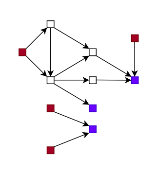
Figure 3: A network graph $G$ with four input nodes in burgundy and three output nodes in violet

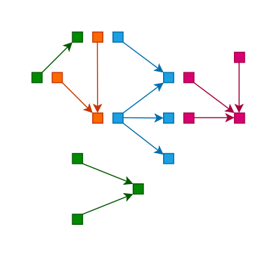
Figure 4: The network graph $G$ split into four network subgraphs with depth of $1$: $G^{1}$ in green, $G^{2}$ in orange, $G^{3}$ in light blue and $G^{4}$ in pink

Proof of Proposition 3.2.

Consider the decomposition of $G$ into $G^{1},G^{2},\dots,G^{\mathsf{L}}$ according to Lemma A.4. Let $\mathsf{W}^{i}$, $\widetilde{\mathsf{W}}^{i}$ be the respective restrictions of $\mathsf{W}$, $\widetilde{\mathsf{W}}$ onto $E(G^{i})$, and $D^{i}$, $\widetilde{D}^{i}$ be the respective restrictions of $D$, $\widetilde{D}$ onto $E(G^{i})$. We construct the following $2\mathsf{L}$ positive SNNs,

$$\Phi^{i}=(G^{i},\mathsf{W}^{i},D^{i})\quad\text{ and }\quad\widetilde{\Phi}^{i}=(G^{i},\widetilde{\mathsf{W}}^{i},\widetilde{D}^{i}),$$

for $i=1,\dots,\mathsf{L}$. Let $V^{i}_{\rm in}$ be the set of input nodes of $G^{i}$ and $V^{i}_{\rm out}$ be the corresponding set of output nodes. Let $t\in\mathbb{R}^{{\rm d}_{\rm in}}$ be a tuple of input firing times for the positive SNNs $\Phi$, $\widetilde{\Phi}$. For each $i=1,\dots,\mathsf{L}$, we write $t_{V^{i}_{\rm in}}$, $\tilde{t}_{V^{i}_{\rm in}}$, to denote the input tuples to $\Phi^{i}$, $\widetilde{\Phi}^{i}$, respectively, and $t_{V^{i}_{\rm out}}$, $\tilde{t}_{V^{i}_{\rm out}}$ to denote the corresponding output tuples. Note that these tuples depend on the given input tuple $t\in\mathbb{R}^{{\rm d}_{\rm in}}$.

Further,

$$\Big{\|}\mathsf{R}(\Phi^{i})\big{(}t_{V^{i}_{\rm in}}\big{)}-\mathsf{R}(\widetilde{\Phi}^{i})\big{(}\tilde{t}_{V^{i}_{\rm in}}\big{)}\Big{\|}_{\ell^{\infty}}\\ \leq\Big{\|}\mathsf{R}(\Phi^{i})\big{(}t_{V^{i}_{\rm in}}\big{)}-\mathsf{R}(\Phi^{i})\big{(}\tilde{t}_{V^{i}_{\rm in}}\big{)}\Big{\|}_{\ell^{\infty}}+\Big{\|}\mathsf{R}(\Phi^{i})\big{(}\tilde{t}_{V^{i}_{\rm in}}\big{)}-\mathsf{R}(\widetilde{\Phi}^{i})\big{(}\tilde{t}_{V^{i}_{\rm in}}\big{)}\Big{\|}_{\ell^{\infty}}.$$ (A.18)

With the graph depth of $G^{i}$ being $1$ (by Lemma A.4), we can apply Lemmas A.2, A.3 to the second term on the RHS of (A.18), resulting in

$$\Big{\|}\mathsf{R}(\Phi^{i})\big{(}\tilde{t}_{V^{i}_{\rm in}}\big{)}-\mathsf{R}(\widetilde{\Phi}^{i})\big{(}\tilde{t}_{V^{i}_{\rm in}}\big{)}\Big{\|}_{\ell^{\infty}}\leq\Big{(}1+\frac{1}{\mathsf{b}^{2}}\Big{)}\|\Phi^{i}-\widetilde{\Phi}^{i}\|_{\ell^{\infty}}.$$ (A.19)

For the first term on the RHS of (A.18), we use Lemma A.1 to obtain

$$\Big{\|}\mathsf{R}(\Phi^{i})\big{(}t_{V^{i}_{\rm in}}\big{)}-\mathsf{R}(\Phi^{i})\big{(}\tilde{t}_{V^{i}_{\rm in}}\big{)}\Big{\|}_{\ell^{\infty}}\leq\|t_{V^{i}_{\rm in}}-\tilde{t}_{V^{i}_{\rm in}}\|_{\ell^{\infty}}.$$ (A.20)

By construction, an input node of $G^{i}$ either originates from an output node of $G^{j}$, for some $j<i$, or an input node of $G$ (see for instance, the graph $G^{4}$ depicted in Figure 4). Subsequently, each component in $t_{V^{i}_{\rm in}}$ is either a component in $t_{V^{j}_{\rm out}}$, or a component in the network input $t$. A similar assertion applies to the corresponding components in $\tilde{t}_{V^{i}_{\rm in}}$. We can then deduce that the RHS of (A.20) is bounded above by

$$\Big{\|}t_{V^{j}_{\rm out}}-\tilde{t}_{V^{j}_{\rm out}}\Big{\|}_{\ell^{\infty}}=\Big{\|}\mathsf{R}(\Phi^{i-1})\big{(}t_{V^{j}_{\rm in}}\big{)}-\mathsf{R}(\widetilde{\Phi}^{i-1})\big{(}\tilde{t}_{V^{j}_{\rm in}}\big{)}\Big{\|}_{\ell^{\infty}},$$

for some $j<i$. However, this quantity resembles the LHS of (A.18). Hence, by replicating the provided reasoning inductively, and combining (A.18), (A.19), we derive

$$\begin{split}\Big{\|}t_{V^{i}_{\rm out}}-\tilde{t}_{V^{i}_{\rm out}}\Big{\|}_{\ell^{\infty}}&=\Big{\|}\mathsf{R}(\Phi^{i})\big{(}t_{V^{i}_{\rm in}}\big{)}-\mathsf{R}(\widetilde{\Phi}^{i})\big{(}\tilde{t}_{V^{i}_{\rm in}}\big{)}\Big{\|}_{\ell^{\infty}}\\ &\leq\sum_{k=1}^{i}\Big{(}1+\frac{1}{\mathsf{b}^{2}}\Big{)}\|\Phi^{k}-\widetilde{\Phi}^{k}\|_{\ell^{\infty}}.\end{split}$$ (A.21)

Let $v\in V_{\rm out}$ be an output node of $G$. Then $v$ is an output node in one of the $G^{i}$, $i=1,\dots,\mathsf{L}$. By Lemma A.4, the edge sets $E(G^{i})$ are mutually disjoint, and collectively, they exhaust the entire edge set $E(G)$ Therefore, from (A.21) we can infer

$$|t_{v}-\tilde{t}_{v}|\leq\sum_{i=1}^{\mathsf{L}}\Big{(}1+\frac{1}{\mathsf{b}^{2}}\Big{)}\|\Phi^{i}-\widetilde{\Phi}^{i}\|_{\ell^{\infty}}\leq\mathsf{L}\cdot\Big{(}1+\frac{1}{\mathsf{b}^{2}}\Big{)}\|\Phi-\widetilde{\Phi}\|_{\ell^{\infty}},$$ (A.22)

where $t_{v}=t_{v}(t)$, $\tilde{t}_{v}=\tilde{t}_{v}(t)$ denote the output firing times at $v$ in $\Phi$, $\tilde{\Phi}$, respectively, given $t\in\mathbb{R}^{{\rm d}_{\rm in}}$. The conclusion (3.2) now follows from (A.22), completing the proof. ∎

A.4 Proof of Theorem 3.6

In the subsequent discussion, the dimension of the zero vector $\vec{0}$ can be inferred from the context. As usual, we start with a necessary lemma.

Lemma A.5.

Let $\Phi=(G,\mathsf{W},D)$ be a positive SNN. Let $\mathsf{b},\mathsf{B}\in(0,\infty)$ be such that for all $(u,v)\in E$, $\mathsf{w}_{(u,v)}\geq\mathsf{b}$ and $d_{(u,v)}\leq\mathsf{B}$. Let $\mathsf{L}$ be the graph depth of $G$. Then

$$\|\mathsf{R}(\Phi)(\vec{0})\|_{\ell^{\infty}}\leq\mathsf{L}\cdot\Big{(}\frac{1}{\mathsf{b}}+\mathsf{B}\Big{)}.$$ (A.23)

Proof.

To begin, we consider the case where $d_{(u,v)}=0$ for all $(u,v)\in E$, and we refer to this specific SNN as $\Phi_{0}$. We make the following observation. Let $v\in V\setminus V_{\rm in}$. Suppose $t_{u}=0$ for all $(u,v)\in E$, and let $t_{v}$ be the corresponding firing time. Then by definition,

$$P_{v}(t_{v})=\sum_{(u,v)\in E}\mathsf{w}_{(u,v)}\varrho(t_{v})=1,$$

from which we obtain

$$t_{v}=\frac{1}{\sum_{(u,v)\in E}\mathsf{w}_{(u,v)}}.$$ (A.24)

Using this, we proceed to derive (A.23) for $\Phi=\Phi_{0}$. For each $u\in V\setminus V_{\rm in}$, let $t_{u}$ be the corresponding firing time at $u$ when the input firing times of $\Phi_{0}$ are set to $\vec{0}$. Let $v\in V_{\rm out}$. Then we can also interpret $t_{v}=t_{v}\big{(}(t_{u})_{(u,v)\in E}\big{)}$. Therefore, an application of Lemma A.1 and the base case result (A.24) grants us

$$|t_{v}\big{(}(t_{u})_{(u,v)\in E}\big{)}| \leq|t_{v}(\vec{0})|+|t_{v}\big{(}(t_{u})_{(u,v)\in E}\big{)}-t_{v}(\vec{0})|$$

$$\leq\frac{1}{\sum_{(u,v)\in E}\mathsf{w}_{(u,v)}}+\|(t_{u})_{(u,v)\in E}\|_{\ell^{\infty}}.$$ (A.25)

Continuing as in the proof of Theorem 3.1, we can find a directed path of synaptic edges, $(v_{N},\dots,v_{0})$, such that $v_{0}=v$, $v_{N}\in V_{\rm in}$, and for each $i=0,\dots,N-1$, it holds that

$$\|(t_{u})_{(u,v_{i})\in E}\|_{\ell^{\infty}}=|t_{v_{i+1}}|.$$

By inductively employing the reasoning in (A.25) along this path, bearing in mind that the input firing times of $\Phi_{0}$ are $\vec{0}$, we acquire

$$|t_{v_{0}}|=|t_{v}|\leq\sum_{i=0}^{N-1}\frac{1}{\sum_{(u,v_{i})\in E}\mathsf{w}_{(u,v_{i})}}\leq\frac{\mathsf{L}}{\mathsf{b}},$$

which in turn implies

$$\|\mathsf{R}(\Phi_{0})(\vec{0})\|_{\ell^{\infty}}\leq\frac{\mathsf{L}}{\mathsf{b}}.$$ (A.26)

Subsequently, in the case of general $\Phi$, it can be deduced from (A.26) and the argument presented in the proof of Proposition 3.2 (with the synaptic weights coinciding) that

$$\|\mathsf{R}(\Phi)(\vec{0})\|_{\ell^{\infty}} \leq\|\mathsf{R}(\Phi_{0})(\vec{0})\|_{\ell^{\infty}}+\|\mathsf{R}(\Phi)(\vec{0})-\mathsf{R}(\Phi_{0})(\vec{0})\|_{\ell^{\infty}}$$

$$\leq\mathsf{L}\cdot\Big{(}\frac{1}{\mathsf{b}}+\|\Phi-\Phi_{0}\|_{\ell^{\infty}}\Big{)}\leq\mathsf{L}\cdot\Big{(}\frac{1}{\mathsf{b}}+\mathsf{B}\Big{)},$$

as wanted. ∎

Proof of Theorem 3.6.

Let $x\in\mathbb{R}^{{\rm d}_{0}}$. Then the inputs of $\Phi$ and $\widetilde{\Phi}$ are $t=(t_{u})_{u\in V_{\rm in}}=A_{\rm in}(x)$ and $\tilde{t}=(\tilde{t}_{u})_{u\in V_{\rm in}}=\tilde{A}_{\rm in}(x)$, respectively, where

$$A_{\rm in}(x)=W_{\rm in}x+b_{\rm in}\quad\text{ and }\quad\tilde{A}_{\rm in}(x)=\widetilde{W}_{\rm in}x+\tilde{b}_{\rm in}.$$ (A.27)

It follows from (A.27) and the estimate (A.7), as well as Proposition 3.2, that

$$\|\mathsf{R}(\Phi)(t)-\mathsf{R}(\widetilde{\Phi})(\tilde{t})\|_{\ell^{\infty}} \leq\|\mathsf{R}(\Phi)(t)-\mathsf{R}(\Phi)(\tilde{t})\|_{\ell^{\infty}}+\|\mathsf{R}(\Phi)(\tilde{t})-\mathsf{R}(\widetilde{\Phi})(\tilde{t})\|_{\ell^{\infty}}$$ (A.28)

$$\leq\|t-\tilde{t}\|_{\ell^{\infty}}+\mathsf{L}\cdot\Big{(}1+\frac{1}{\mathsf{b}^{2}}\Big{)}\|\Phi-\widetilde{\Phi}\|_{\ell^{\infty}}$$

$$\leq\|W_{\rm in}-\widetilde{W}_{\rm in}\|_{F}\|x\|_{\ell^{2}}+\|b_{\rm in}-\tilde{b}_{\rm in}\|_{\ell^{\infty}}+\mathsf{L}\cdot\Big{(}1+\frac{1}{\mathsf{b}^{2}}\Big{)}\|\Phi-\widetilde{\Phi}\|_{\ell^{\infty}}$$

$$\leq{\rm d}_{0}^{\frac{1}{2}}\|W_{\rm in}-\widetilde{W}_{\rm in}\|_{F}\|x\|_{\ell^{\infty}}+\mathsf{L}\cdot\Big{(}1+\frac{1}{\mathsf{b}^{2}}\Big{)}\|\Phi-\widetilde{\Phi}\|_{\ell^{\infty}}+\|b_{\rm in}-\tilde{b}_{\rm in}\|_{\ell^{\infty}}$$

Denote $z=\mathsf{R}(\Phi)(t)$, $\tilde{z}=\mathsf{R}(\widetilde{\Phi})(\tilde{t})$. We can write

$$\begin{split}\|\mathsf{R}(\Psi)(x)-\mathsf{R}(\widetilde{\Psi})(x)\|_{\ell^{\infty}}&=\|A_{\rm out}(z)-\tilde{A}_{\rm out}(\tilde{z})\|_{\ell^{\infty}}\\ &\leq\|A_{\rm out}(z)-A_{\rm out}(\tilde{z})\|_{\ell^{\infty}}+\|A_{\rm out}(\tilde{z})-\tilde{A}_{\rm out}(\tilde{z})\|_{\ell^{\infty}}\\ &=T_{1}+T_{2},\end{split}$$ (A.29)

where $T_{1}\coloneqq\|A_{\rm out}(z)-A_{\rm out}(\tilde{z})\|_{\ell^{\infty}}$, $T_{2}\coloneqq\|A_{\rm out}(\tilde{z})-\tilde{A}_{\rm out}(\tilde{z})\|_{\ell^{\infty}}$. Applying (A.28) to $T_{1}$, we get

$$T_{1}\leq{\rm d}_{\rm out}^{\frac{1}{2}}\|W_{\rm out}\|_{F}\bigg{(}{\rm d}_{0}^{\frac{1}{2}}\|W_{\rm in}-\widetilde{W}_{\rm in}\|_{F}\|x\|_{\ell^{\infty}}+\mathsf{L}\cdot\Big{(}1+\frac{1}{\mathsf{b}^{2}}\Big{)}\|\Phi-\widetilde{\Phi}\|_{\ell^{\infty}}+\|b_{\rm in}-\tilde{b}_{\rm in}\|_{\ell^{\infty}}\bigg{)}.$$

Further, given

$$A_{\rm out}(x)=W_{\rm out}x+b_{\rm out}\quad\text{ and }\quad\tilde{A}_{\rm out}(x)=\widetilde{W}_{\rm out}x+\tilde{b}_{\rm out},$$

we can also similarly obtain

$$T_{2} \leq{\rm d}_{\rm out}^{\frac{1}{2}}\|W_{\rm out}-\widetilde{W}_{\rm out}\|_{F}\|\tilde{z}\|_{\ell^{\infty}}+\|b_{\rm out}-\tilde{b}_{\rm out}\|_{\ell^{\infty}}$$

$$\leq{\rm d}_{\rm out}^{\frac{1}{2}}\|W_{\rm out}-\widetilde{W}_{\rm out}\|_{F}\Big{(}\|\mathsf{R}(\widetilde{\Phi})(\tilde{t})-\mathsf{R}(\widetilde{\Phi})(\vec{0})\|_{\ell^{\infty}}+\|\mathsf{R}(\widetilde{\Phi})(\vec{0})\|_{\ell^{\infty}}\Big{)}+\|b_{\rm out}-\tilde{b}_{\rm out}\|_{\ell^{\infty}}$$

$$\leq{\rm d}_{\rm out}^{\frac{1}{2}}\|W_{\rm out}-\widetilde{W}_{\rm out}\|_{F}\Big{(}\|\tilde{t}\|_{\ell^{\infty}}+\mathsf{L}\cdot\Big{(}\frac{1}{\mathsf{b}}+\mathsf{B}\Big{)}\Big{)}+\|b_{\rm out}-\tilde{b}_{\rm out}\|_{\ell^{\infty}}$$

$$\leq{\rm d}_{\rm out}^{\frac{1}{2}}\|W_{\rm out}-\widetilde{W}_{\rm out}\|_{F}\Big{(}{\rm d}_{0}^{\frac{1}{2}}\|\widetilde{W}_{\rm in}\|_{F}\|x\|_{\ell^{\infty}}+\|\tilde{b}_{\rm in}\|_{\ell^{\infty}}+\mathsf{L}\cdot\Big{(}\frac{1}{\mathsf{b}}+\mathsf{B}\Big{)}\Big{)}+\|b_{\rm out}-\tilde{b}_{\rm out}\|_{\ell^{\infty}},$$

where we have used (A.7) and Lemma A.5 in the third inequality above. Substituting these estimates back into (A.29), we acquire the desired conclusion for the theorem. ∎

A.5 Proof of Theorem 4.3

A standard learning result employing covering numbers is as follows.

Theorem A.6 ([38, Exercise 3.31]).

Let ${\rm d}_{0},m\in\mathbb{N}$. Let $\mathcal{H}$ be a hypothesis set of functions from $[0,1]^{{\rm d}_{0}}$ to $[c_{\rm min},c_{\rm max}]$, where $c_{\rm min},c_{\rm max}\in\mathbb{R}$. Let $\mathcal{D}$ be a distribution on $[0,1]^{{\rm d}_{0}}\times[c_{\rm min},c_{\rm max}]$. Let, for $m\in\mathbb{N}$, $S\sim\mathcal{D}^{m}$ be a sample. Then, for all $\varepsilon>0$

$$\mathbb{P}\Big{(}\sup_{h\in\mathcal{H}}|\mathcal{R}(h)-\widehat{\mathcal{R}}_{S}(h)|\geq\varepsilon\Big{)}\leq 2\mathcal{N}\Big{(}\mathcal{H},\frac{\varepsilon}{8(c_{\rm max}-c_{\rm min})},L^{\infty}([0,1]^{{\rm d}_{0}})\Big{)}\mathrm{exp}\Big{(}\frac{-m\varepsilon^{2}}{2(c_{\rm max}-c_{\rm min})^{4}}\Big{)}.$$

We show below that Theorem A.6 and (4.7) imply Theorem 4.3.

Proof of Theorem 4.3.

Set, for $m\in\mathbb{N}$ satisfying (4.8),

$$\varepsilon(\delta)\coloneqq\sqrt{\frac{2(\mathsf{M}\log(m\lceil 16\mathsf{B}L^{\star}\rceil)+\log(2/\delta))}{m}}\leq 1,$$

then by Theorem A.6 the statement of this theorem follows if

$$2\mathcal{N}\Big{(}\mathsf{R}_{[0,1]}(\mathcal{P}_{\rm SNN}^{\star}(G,\vec{{\rm d}};\mathsf{b},\mathsf{B})),\frac{\varepsilon(\delta)}{8},L^{\infty}([0,1]^{{\rm d}_{0}})\Big{)}\mathrm{exp}\Big{(}\frac{-m\varepsilon(\delta)^{2}}{2}\Big{)}\leq\delta.$$

Since, by definition

$$\mathrm{exp}\Big{(}\frac{-m\varepsilon(\delta)^{2}}{2}\Big{)}=\frac{\delta}{2}\mathrm{exp}\Big{(}-\mathsf{M}\log\Big{(}m\Big{\lceil}16\mathsf{B}L^{\star}\Big{\rceil}\Big{)}\Big{)},$$

we can conclude the theorem if

$$\mathcal{N}\Big{(}\mathsf{R}_{[0,1]}(\mathcal{P}_{\rm SNN}^{\star}(G,\vec{{\rm d}};\mathsf{b},\mathsf{B})),\frac{\varepsilon(\delta)}{8},L^{\infty}([0,1]^{{\rm d}_{0}})\Big{)}\leq\mathrm{exp}\Big{(}\mathsf{M}\log\Big{(}m\Big{\lceil}16\mathsf{B}L^{\star}\Big{\rceil}\Big{)}\Big{)}.$$ (A.30)

Let us have a look at the left-hand side of (A.30). Building upon the rationale given in (4.7), it holds that

$$\begin{split}\log\Big{(}\mathcal{N}\Big{(}\mathsf{R}_{[0,1]}(\mathcal{P}_{\rm SNN}^{\star}(G,\vec{{\rm d}};\mathsf{b},\mathsf{B})),\frac{\varepsilon(\delta)}{8},L^{\infty}([0,1]^{{\rm d}_{0}})\Big{)}\Big{)}&\leq\mathsf{M}\log\Big{(}\Big{\lceil}\frac{16\mathsf{B}L^{\star}}{\varepsilon(\delta)}\Big{\rceil}\Big{)}\\ &\leq\mathsf{M}\log\Big{(}m\Big{\lceil}16\mathsf{B}L^{\star}\Big{\rceil}\Big{)},\end{split}$$ (A.31)

where we have used that $\lceil 1/(\varepsilon(\delta))\rceil\leq\lceil\sqrt{m}\rceil\leq m$. Exponentiating (A.31) yields (A.30) and thus completes the proof. ∎

A.6 Proof of Lemma 5.1

We begin by constructing $\Phi^{\rm min}_{\varepsilon}=(G,\mathsf{W}^{\rm min}_{\varepsilon},D^{\rm min}_{\varepsilon})$ as follows. We take $G$ to be a graph with ${\rm d}_{0}$ input nodes $u_{1},\dots,u_{{\rm d}_{0}}$ and one output node $v$. Let $\mathsf{W}^{\rm min}_{\varepsilon}$ consist of $\mathsf{w}_{(u_{i},v)}=\varepsilon^{-1}$ for $i=1,\dots,{\rm d}_{0}$. Let all the delays be zero, i.e. $d_{(u_{i},v)}=0$, for $i=1,\dots,{\rm d}_{0}$. Finally, we formalize the structure of $\Psi^{\rm min}_{\varepsilon}$ by defining $A_{\rm in}:\mathbb{R}^{{\rm d}_{0}}\to\mathbb{R}^{{\rm d}_{0}}$, $A_{\rm out}:\mathbb{R}\to\mathbb{R}$ as $A_{\rm in}={\rm Id}^{{\rm d}_{0}\times{\rm d}_{0}}$, $A_{\rm out}={\rm Id}^{1\times 1}$, respectively.

To show that $\Psi^{\rm min}_{\varepsilon}$ fulfills (5.1), we first calculate the output firing time $t_{v}$ by $\Phi^{\rm min}_{\varepsilon}$ from the input firing times $t_{u_{i}}$. Suppose, without loss of generality, that

$$t_{u_{1}}=\min\{t_{u_{i}}\colon i=1,\dots,{\rm d}_{0}\}.$$

The potential at $v$ then takes the form (2.2)

$$P_{v}(t)=\sum_{i=1}^{{\rm d}_{0}}\varepsilon^{-1}\varrho(t-t_{u_{i}}).$$ (A.32)

Since all terms on the right-hand side of (A.32) are non-negative, we deduce

$$P_{v}(t_{u_{1}}+\varepsilon)\geq\varepsilon^{-1}\varrho(\varepsilon)=1.$$

It follows that the firing time $t_{v}$ of $v$ is not larger than $t_{u_{1}}+\varepsilon$. On the other hand, $P_{v}(t_{u_{1}})=0$. Therefore, $t_{v}\in(t_{u_{1}},t_{u_{1}}+\varepsilon]$, by the continuity of $P_{v}$ and the intermediate value theorem. We conclude that, for $x_{1},\dots,x_{{\rm d}_{0}}\in\mathbb{R}$,

$$|\mathsf{R}(\Psi^{\rm min}_{\varepsilon})(x_{1},\dots,x_{{\rm d}_{0}})-\min\{x_{1},\dots,x_{{\rm d}_{0}}\}|\\ =|(A_{\rm out}\circ\Phi^{\rm min}_{\varepsilon}\circ A_{\rm in})(x_{1},\dots,x_{{\rm d}_{0}})-\min\{x_{1},\dots,x_{{\rm d}_{0}}\}|\leq\varepsilon,$$

which shows (5.1). It remains to observe that ${\rm Size}(\Psi^{\rm min}_{\varepsilon})=2{\rm d}_{0}+1$, as per the construction. ∎

A.7 Proof of Lemma 5.3

We create $\Psi_{a,b,c,d,\varepsilon}=(A_{\rm in},\Phi,A_{\rm out})$ as follows. We define $A_{\rm in}\colon\mathbb{R}^{{\rm d}_{0}}\to\mathbb{R}^{2}$ to be such that

$$A_{\rm in}(x)=\begin{pmatrix}-a^{\top}x-b\\ 0\end{pmatrix},$$ (A.33)

and $A_{\rm out}\colon\mathbb{R}\to\mathbb{R}$ such that $A_{\rm out}(x)=-cx+d$. In constructing $\Phi=(G,\mathsf{W},D)$, we follow the structure of $\Phi^{\rm min}_{\varepsilon}$ in the proof of Lemma 5.1. Namely, we let $G$ consist of two synapses, $(u_{1},v)$, $(u_{2},v)$, with $\mathsf{w}_{(u_{i},v)}=\varepsilon^{-1}$ and $d_{(u_{i},v)}=0$. To see that $\Psi_{a,b,c,d,\varepsilon}$ satisfies (5.2), we note, as argued in the proof of Lemma 5.1,

$$|\mathsf{R}(\Phi)(t_{1},t_{2})-\min\{t_{1},t_{2}\}|\leq\varepsilon;$$

therefore,

$$\Big{|}A_{\rm out}\circ\mathsf{R}(\Phi)(t_{1},t_{2})-\Big{(}-c\cdot\big{(}\min\{t_{1},t_{2}\}\big{)}+d\Big{)}\Big{|}\\ =\Big{|}A_{\rm out}\circ\mathsf{R}(\Phi)(t_{1},t_{2})-\Big{(}c\cdot\big{(}\max\{-t_{1},-t_{2}\}\big{)}+d\Big{)}\Big{|}\leq|c|\varepsilon.$$ (A.34)

Combining (A.33), (A.34), we obtain (5.2).

Finally, it is straightforward to see that ${\rm Size}(\Psi_{a,b,c,d,\varepsilon})\leq{\rm d}_{0}+5$. Moreover, the weights of $\Psi_{a,b,c,d,\varepsilon}$ are bounded above in absolute value by $\max\{1/\varepsilon,\|a\|_{\ell^{\infty}},|b|,|c|,|d|\}$, and the synaptic weights are bounded below by ${1}/{\varepsilon}$.

A.8 Proof of Theorem 5.4

For $M\in\mathbb{N}$, recall the set $H_{M}$ defined in (5.3). Then by the well-known result [30, Theorem 1], $\bigcup_{M\in\mathbb{N}}H_{M}$ is dense in $\mathcal{C}(\Omega)$. On the other hand, it is evident from Lemma 5.3 and Definition 2.11 that each $H_{M}$ is contained in the closure of the set of all realizations of affine SNNs. The result now follows. ∎

A.9 Proof of Theorem 5.7

We first prove that affine SNNs with relatively moderate size can effectively approximate the basis elements $\phi_{\eta}$ of $V_{\mathcal{T}}$, in the following lemma.

Lemma A.7.

Let ${\rm d}_{0}\in\mathbb{N}$, and let $\Omega\subset\mathbb{R}^{{\rm d}_{0}}$ be compact. Let $\mathcal{T}$ be a regular triangulation of $\Omega$ with node set $\mathcal{N}$. Let $\varepsilon>0$. Then for each node $\eta\in\mathcal{N}$ such that $G(\eta)$ is convex, there exists an SNN $\Psi_{\varepsilon}^{\eta}$ such that, for all $x\in\Omega$

$$|\mathsf{R}(\Psi_{\varepsilon}^{\eta})(x)-\phi_{\eta}(x)|\leq\varepsilon.$$

Moreover,

$${\rm Size}(\Psi^{\eta}_{\varepsilon})\leq({\rm d}_{0}+2)\#T(\eta)+6,$$

all the weights in $\Psi_{\varepsilon}^{\eta}$ are bounded above in absolute value by

$$\max\big{\{}1,1/h_{\min}(\mathcal{T}),C{\rm d}_{0}/h_{\min}(\mathcal{T}),3/\varepsilon\big{\}}$$

for some $C=C(\Omega)>0$, and all the synaptic weights are bounded below by $\min\{1,{3}/{\varepsilon}\}$.

Proof.

Since for each $\tau\in T(\eta)$, $g_{\tau}$ is globally affine, it takes the form, $g_{\tau}(x)=a_{\tau}^{\top}x+b_{\tau}$, where $a_{\tau}\in\mathbb{R}^{{\rm d}_{0}}$, $b_{\tau}\in\mathbb{R}$. We build an affine SNN $\Psi^{\eta}_{3\varepsilon}=(A_{\rm in},\Phi,A_{\rm out})$ as follows. Let $A_{\rm out}\colon\mathbb{R}^{2}\to\mathbb{R}$ be such that, $A_{\rm out}(x,y)=x-1-y$, and $A_{\rm in}\colon\mathbb{R}^{{\rm d}_{0}}\to\mathbb{R}^{\#T(\eta)+1}$ such that

$$A_{\rm in}(x)=\begin{pmatrix}\big{(}a_{\tau}^{\top}x+b_{\tau}\big{)}_{\tau\in T(\eta)}\\ 0\end{pmatrix}.$$

Next, we consider $\Phi=(G,\mathsf{W},D)$, a positive SNN where $G$ comprises $\#T(\eta)+1$ input nodes, labeled $u_{0},u_{\tau}$, for $\tau\in T(\eta)$, $2$ output nodes, labeled $v_{1}$, $v_{2}$, and $1$ intermediate node $w$, along with $\#T(\eta)+3$ synaptic edges. The synaptic edges and their weights are,

$$\mathsf{w}_{(u_{\tau},w)}=\mathsf{w}_{(w,v_{2})}=\mathsf{w}_{(u_{0},v_{2})}=\varepsilon^{-1},\quad\text{ and }\quad\mathsf{w}_{(w,v_{1})}=1.$$ (A.35)

Let all the corresponding delays be zero. Then, given input firing times $((t_{u_{\tau}})_{\tau\in T(\eta)},t_{u_{0}})$, we can deduce from (A.35) and the reasoning provided in the proof of Lemma 5.1 that

$$|t_{w}-\min\{t_{u_{\tau}}\colon\tau\in T(\eta)\}|\leq\varepsilon,$$

and $|t_{v_{2}}-\min\{t_{w},t_{u_{0}}\}|\leq\varepsilon$. Therefore,

$$\begin{split}|t_{v_{1}}-(\min\{t_{u_{\tau}}\colon\tau\in T(\eta)\}+1)|&\leq\varepsilon,\\ |t_{v_{2}}-\min\{t_{u_{0}},\min\{t_{u_{\tau}}\colon\tau\in T(\eta)\}\}|&\leq 2\varepsilon.\end{split}$$ (A.36)

Integrating (A.36) with the specifics given to $A_{\rm in}$, $A_{\rm out}$, we conclude for $x\in\Omega$,

$$|\mathsf{R}(\Psi^{\eta}_{3\varepsilon})(x)-\big{(}\min_{\tau\in T(\eta)}(a_{\tau}^{\top}x+b_{\tau})-\min\{0,\min_{\tau\in T(\eta)}(a_{\tau}^{\top}x+b_{\tau})\}\big{)}|\leq 3\varepsilon.$$

It should be now routine to check that ${\rm Size}(\Psi^{\eta}_{3\varepsilon})\leq({\rm d}_{0}+2)\#T(\eta)+6$ and that every synaptic weight in $\Psi^{\eta}_{3\varepsilon}$ is bounded below by $\min\{1,1/\varepsilon\}$. As for the remaining weights, it can be inferred from (5.4) and the the fact that $g_{\tau}=\phi_{\eta}$ on $\tau$ that

$$\|a_{\tau}\|_{\ell^{\infty}}\leq 1/h_{\rm min}(\mathcal{T}).$$ (A.37)

Additionally, it also follows from (5.4) that $g_{\tau}(x_{\tau}^{\star})=0$ for some $x_{\tau}^{\star}\in\Omega$. Thus

$$|b_{\tau}|\leq|a_{\tau}^{\top}x_{\tau}^{\star}|\leq{\rm d}_{0}\,\sup\{|x|\colon x\in\Omega\}/h_{\min}(\mathcal{T}).$$ (A.38)

Therefore, by combining (A.37), (A.38), we conclude the final assertion of the lemma with $1/\varepsilon$ instead of $3/\varepsilon$. Finally, the result follows by substituting $\varepsilon$ by $\varepsilon/3$. ∎

Theorem 5.7 now follows as an immediate consequence of Lemma A.7.

Proof of Theorem 5.7.

Let $f\in V_{\mathcal{T}}$. Since $(\phi_{\eta})_{\eta\in\mathcal{N}}$ is a basis of $V_{\mathcal{T}}$ satisfying (5.4), we can write

$$f(x)=\sum_{\eta\in\mathcal{N}}f(\eta)\phi_{\eta}(x).$$

For each $\eta\in\mathcal{N}$, following an argument presented in the proof of Lemma A.7, we construct an affine SNN $\Psi^{\eta}_{\varepsilon}$ that guarantees for all $x\in\Omega$,

$$|\mathsf{R}(\Psi^{\eta}_{\varepsilon})(x)-f(\eta)\phi_{\eta}(x)|\leq|f(\eta)|\varepsilon.$$

Let $\Psi^{f}_{\varepsilon}\coloneqq\bigoplus_{\eta\in\mathcal{N}}\Psi^{\eta}_{\varepsilon}$. The theorem now follows directly from an application of Lemma 2.12 and the triangle inequality. ∎

A.10 Proof of Theorem 5.9

We cite the following known result, which we will use to demonstrate Theorem 5.9.

Proposition A.8 ([9, Proposition 1]).

Let ${\rm d}_{0}\in\mathbb{N}$ and $\Omega\subset\mathbb{R}^{{\rm d}_{0}}$ be a compact domain. Let $s\in\{1,2\}$. Let $\mathcal{T}$ be a regular triangulation of $\Omega$. Then for every $f\in W^{s,\infty}(\Omega)$, there exist $g=\sum_{\eta\in\mathcal{N}}c_{\eta}\phi_{\eta}$ and constants $C_{1},C_{2}=C_{2}(\mathcal{T},{\rm d}_{0})>0$, such that $|c_{\eta}|\leq C_{1}\|f\|_{L^{\infty}(\Omega)}$, and that

$$\|f-g\|_{L^{\infty}(\Omega)}\leq C_{2}\cdot(h_{\max}(\mathcal{T}))^{s}\|f\|_{W^{s,\infty}(\Omega)}.$$

In addition, the constant $C_{2}(\mathcal{T},{\rm d}_{0})$ depends on $\mathcal{T}$ only through the so-called shape coefficient $h_{\rm max}(\mathcal{T})/h_{\rm min}(\mathcal{T})$, i.e., $C_{2}(\mathcal{T},{\rm d}_{0})=C_{2}(h_{\rm max}(\mathcal{T})/h_{\rm min}(\mathcal{T}),{\rm d}_{0})$.

Proof of Theorem 5.9.

In what follows, the majorant constant $C$ is subject to change meaning from one instance to the next, and its parametric dependence, if present, will be explicitly specified. Since $\Omega$ is admissible, we can choose for $N\in\mathbb{N}$ a triangulation $\mathcal{T}_{N}$ for which (5.6) holds. Therefore, by Proposition A.8, there exists $g=\sum_{\eta\in\mathcal{N}}c_{\eta}\phi_{\eta}$ satisfying

$$\|f-g\|_{L^{\infty}(\Omega)}\leq CN^{-s/{\rm d}_{0}}\|f\|_{W^{s,\infty}(\Omega)},$$ (A.39)

where $C=C({\rm d}_{0})$ only. In turn, since $g\in V_{\mathcal{T}_{N}}$, Theorem 5.7 implies the existence of an affine SNN $\Psi^{g}_{N}$ such that

$$\|\mathsf{R}(\Psi^{g}_{N})-g\|_{L^{\infty}(\Omega)}\leq CN\max_{\eta\in\mathcal{N}(\mathcal{T}_{N})}|c_{\eta}|N^{-s/{\rm d}_{0}-1}\leq CN^{-s/{\rm d}_{0}}\|f\|_{L^{\infty}(\Omega)}.$$ (A.40)

By renaming $\Psi^{g}_{N}$ to $\Psi^{f}_{N}$ and combining (A.39), (A.40), we obtain (5.7). The size of $\Psi^{f}_{N}$ and its associated weights can now be determined by applying the conclusions of Theorem 5.7 with $\varepsilon$ in place of $N^{-s/{\rm d}_{0}-1}$. ∎

A.11 Proof of Theorem 5.11

Before proceeding, we introduce a key result derived from [3, Theorem 1] and [10, Proposition 2.2], which sets the stage for our analysis.

Theorem A.9.

Let ${\rm d}_{0}\in\mathbb{N}$. There is a universal constant $\kappa>0$ such that the following holds. For every $K>0$, every $f\in\Gamma_{K}$, and every $M\in\mathbb{N}$, there exists an element $g\in H_{8M}$ (as in (5.3)) such that

$$\sup_{x\in\overline{B(0,1)}}|f(x)-g(x)|\leq\frac{\kappa\,{\rm d}_{0}^{\frac{1}{2}}K}{\sqrt{M}},$$

where $\overline{B(0,1)}$ denotes the closed unit ball in $\mathbb{R}^{{\rm d}_{0}}$. Furthermore, for all $i=1,\dots,8M$, $\|a_{i}\|_{\ell^{\infty}},|b_{i}|,|c_{i}|,|d_{i}|$ in the definition of $g$ via (5.3) can be chosen so that

$$\|a_{i}\|_{\ell^{\infty}},|b_{i}|,|c_{i}|,|d_{i}|\leq C\sqrt{K},$$

for some $C>0$.

In the forthcoming discussion, all majorant constants are universal, and the meaning of the analytic constants $C,c>0$ may vary between different instances.

Proof of Theorem 5.11.

By Theorem A.9, there exist constant $\kappa>0$ and $a_{i}\in\mathbb{R}^{{\rm d}_{0}},b_{i},c_{i},d_{i}\in\mathbb{R}$ for $i=1,\dots,8M$ such that $\|a_{i}\|_{\ell^{\infty}},|b_{i}|,|c_{i}|,|d_{i}|\leq C\sqrt{K}$, for some $C>0$, and

$$\sup_{x\in\overline{B(0,1)}}\Big{|}f(x)-\sum_{i=1}^{8M}c_{i}\max\{a_{i}^{\top}x+b_{i},0\}+d_{i}\Big{|}\leq\frac{\kappa\,{\rm d}_{0}^{\frac{1}{2}}K}{\sqrt{M}}.$$ (A.41)

On the other hand, by using Lemma 5.3 and performing repeated additions of affine SNNs, we can construct an affine SNN $\Psi$ such that

$$\sup_{x\in\overline{B(0,1)}}\Big{|}\Psi(x)-\sum_{i=1}^{8M}c_{i}\max\{a_{i}^{\top}x+b_{i},0\}+d_{i}\Big{|}\leq\frac{\kappa K}{\sqrt{M}}.$$ (A.42)

Letting $\Psi^{f}_{M}=\Psi$, we infer from (A.41), (A.42) that

$$\sup_{x\in\overline{B(0,1)}}\Big{|}\Psi^{f}_{M}(x)-f(x)\Big{|}\leq\frac{\kappa K\cdot({\rm d}_{0}^{\frac{1}{2}}+1)}{\sqrt{M}}\leq\frac{2\kappa\,{\rm d}_{0}^{\frac{1}{2}}K}{\sqrt{M}}.$$

Hence, we can set $\nu=2\kappa$. In addition, it is readily seen from the conclusions of Lemmas 2.12, 5.3 and (A.42) that ${\rm Size}(\Psi^{f}_{M})\leq C{\rm d}_{0}M$, that all the weights in $\Psi^{f}_{M}$ can be bounded above by $C\cdot(M^{3/2}/\sqrt{K}+\sqrt{K})$, and all of its synaptic weights can be bounded below by $cM^{3/2}/\sqrt{K}$, for some $C,c>0$. This completes the proof. ∎

A.12 Proof of Theorem 6.1

In the following discussion, the majorant constant $C>0$ is a universal constant, though its value may vary from one instance to the next.

For each $m\in\mathbb{N}$, we let $\varepsilon_{m}\coloneqq m^{{-1}/(\kappa_{\mathsf{M}}+4)}$. Let $\delta^{\prime}>0$. Then under the assumption (6.1), we have the existences of $g_{m}$, depending on $\delta^{\prime}$, such that

$$\|g_{m}-f\|_{L^{\infty}(\Omega)}\leq m^{{-1}/(\kappa_{\mathsf{M}}+4)}+\delta^{\prime}.$$ (A.43)

Therefore, it follows directly from the definition of empirical risk minimizer and (A.43) that

$$\widehat{\mathcal{R}}_{S}(f_{S})\leq\widehat{\mathcal{R}}_{S}(g_{m})\leq\frac{1}{m}\sum_{i=1}^{m}|f(x_{i})-g_{m}(x_{i})|^{2}\leq m^{{-2}/(\kappa_{\mathsf{M}}+4)}+2\delta^{\prime}.$$ (A.44)

Next, we consider the quantity

$$I(\varepsilon_{m})\coloneqq\sqrt{\frac{2\big{(}\mathsf{M}(\varepsilon_{m})\log(m\lceil 16\mathsf{B}(\varepsilon_{m})L^{\star}(\varepsilon_{m})\rceil)+\log(2/\delta)\big{)}}{m}},$$

where, recall from (4.6) that

$$L^{\star}(\varepsilon_{m})\\ \coloneqq{\rm d}_{\rm out}(\varepsilon_{m})\Big{(}2\mathsf{B}(\varepsilon_{m})\Big{(}{\rm d}_{\rm in}^{\frac{1}{2}}(\varepsilon_{m}){\rm d}_{0}+1\Big{)}+\mathsf{B}(\varepsilon_{m})\mathsf{L}(\varepsilon_{m})\Big{(}2+\frac{1}{\mathsf{b}^{2}(\varepsilon_{m})}\Big{)}+\frac{\mathsf{L}(\varepsilon_{m})}{\mathsf{b}(\varepsilon_{m})}\Big{)}+1,$$

and $\mathsf{L}(\varepsilon_{m})$ represents the graph depth $G(\varepsilon_{m})$. Since

$$\max\{{\rm d}_{\rm out}(\varepsilon_{m}),{\rm d}_{\rm in}^{\frac{1}{2}}(\varepsilon_{m}){\rm d}_{0},\mathsf{L}(\varepsilon_{m})\}\leq\mathsf{M}(\varepsilon_{m})\leq\varepsilon_{m}^{-\kappa_{\mathsf{M}}},$$

by definition, and $\varepsilon_{m}^{\kappa_{\mathsf{B}}}\leq\mathsf{b}(\varepsilon_{m})\leq 1\leq\mathsf{B}(\varepsilon_{m})\leq\varepsilon_{m}^{-\kappa_{\mathsf{B}}}$, we acquire

$$L^{\star}(\varepsilon_{m})\leq Cm^{(2\kappa_{\mathsf{M}}+3\kappa_{\mathsf{B}})/(\kappa_{\mathsf{M}}+4)},$$

which subsequently implies

$$I(\varepsilon_{m})\leq C\cdot\Big{(}m^{-2/(\kappa_{\mathsf{M}}+4)}\sqrt{\lambda\log(m)}+\sqrt{\frac{\log(2/\delta)}{m}}\Big{)}$$ (A.45)

where $\lambda\coloneqq(3\kappa_{\mathsf{M}}+4\kappa_{\mathsf{B}}+4)/(\kappa_{\mathsf{M}}+4)$. By applying Theorem 4.3, alongside (A.44), (A.45), we can infer that, with probability at least $1-\delta$,

$$\mathcal{R}(f_{S})\leq\widehat{\mathcal{R}}_{S}(f_{S})+I(\varepsilon_{m})\leq C\cdot\Big{(}m^{-2/(\kappa_{\mathsf{M}}+4)}\sqrt{\lambda\log(m)}+\sqrt{\frac{\log(2/\delta)}{m}}\Big{)}+2\delta^{\prime}.$$ (A.46)

Letting $\delta^{\prime}\to 0$, we obtain from (A.46)

$$\mathcal{R}(f_{S})\leq C\max\big{\{}1,\sqrt{\kappa_{\mathsf{B}}}/\sqrt{\kappa_{\mathsf{M}}}\big{\}}\Big{(}m^{-2/(\kappa_{\mathsf{M}}+4)}\sqrt{\log(m)}+\sqrt{\frac{\log(2/\delta)}{m}}\Big{)}$$

as wanted. ∎

Appendix B SNNs with general responses

Let $\Phi=(G,\mathsf{W},D,\widetilde{\mathcal{E}})$ be an SNN, where the synaptic weights $\mathsf{w}_{(u,v)}\geq 0$, synaptic delays $d_{(u,v)}\geq 0$, but the response $\tilde{\varepsilon}_{(u,v)}$ adopts the form of (2.3), i.e. $\tilde{\varepsilon}_{(u,v)}(t)=s_{(u,v)}\varrho(t)$, where $\delta=\infty$, and $s_{(u,v)}\in\{\pm 1\}$. In this case, the neuron potential at $v\in V\setminus V_{\rm in}$ is then given by $\tilde{P}_{v}$ in (2.4). The following condition, first identified in [49], then guarantees the existence of the network output firing times $(t_{v})_{v\in V_{\rm out}}$ for each tuple of input firing times $(t_{u})_{u\in V_{\rm in}}$:

$$\sum_{(u,v)\in E}\mathsf{w}_{(u,v)}s_{(u,v)}>0.$$ (B.1)

We provide an example to illustrate that, despite this, (B.1) is not enough to ensure the continuity of output firing times as functions of input firing times.

Example B.1.

Consider an SNN $\Phi=(G,\mathsf{W},D,\widetilde{\mathcal{E}})$ with three input neurons $u_{1},u_{2},u_{3}$ presynaptic to one output neuron $v$. Let $\mathsf{w}_{(u_{1},v)}=\mathsf{w}_{(u_{2},v)}=\mathsf{w}_{(u_{3},v)}=1$. Let $s_{(u_{1},v)}=-s_{(u_{2},v)}=s_{(u_{3},v)}=1$. Let $d_{(u_{1},v)}=d_{(u_{2},v)}=d_{(u_{3},v)}=0$. Then for every $t\in\mathbb{R}$

$$\tilde{P}_{v}(t)=\varrho(t-t_{u_{1}})-\varrho(t-t_{u_{2}})+\varrho(t-t_{u_{3}}).$$

Observe that

$$\sum_{i=1}^{3}\mathsf{w}_{(u_{i},v)}s_{(u_{i},v)}>0.$$

Therefore, by (B.1), $t_{v}$ exists, as a function of $(t_{u_{i}})_{i=1}^{3}$. However, $t_{v}(t_{u_{1}},t_{u_{2}},t_{u_{3}})$ is discontinuous at $(t_{u_{1}},t_{u_{2}},t_{u_{3}})=(0,1,2)$. Indeed, for $\varepsilon>0$, the firing time at $(t_{u_{1}},t_{u_{2}},t_{u_{3}})=(0,1+\varepsilon,2)$ is $t_{v}=1$, while the firing time at $(t_{u_{1}},t_{u_{2}},t_{u_{3}})=(0,1-\varepsilon,2)$ is $2+\varepsilon$.

References

- [1] Moshe Abeles. Role of the cortical neuron: integrator or coincidence detector? Israel journal of medical sciences, 18(1):83–92, 1982.
- [2] Martin Anthony and Peter L Bartlett. Neural network learning: Theoretical foundations, volume 9. cambridge university press Cambridge, 1999.
- [3] Andrew R Barron. Neural net approximation. In Proc. 7th Yale workshop on adaptive and learning systems, volume 1, pages 69–72, 1992.
- [4] Andrew R. Barron. Universal approximation bounds for superpositions of a sigmoidal function. IEEE Trans. Inform. Theory, 39(3):930–945, 1993.
- [5] Mikhail Belkin, Daniel Hsu, Siyuan Ma, and Soumik Mandal. Reconciling modern machine-learning practice and the classical bias–variance trade-off. Proceedings of the National Academy of Sciences, 116(32):15849–15854, 2019.
- [6] Yoshua Bengio, Ian Goodfellow, and Aaron Courville. Deep learning, volume 1. MIT press Cambridge, MA, USA, 2017.
- [7] Julius Berner, Philipp Grohs, and Arnulf Jentzen. Analysis of the generalization error: Empirical risk minimization over deep artificial neural networks overcomes the curse of dimensionality in the numerical approximation of black–scholes partial differential equations. SIAM Journal on Mathematics of Data Science, 2(3):631–657, 2020.
- [8] Julius Berner, Philipp Grohs, Gitta Kutyniok, and Philipp Petersen. The modern mathematics of deep learning. arXiv preprint arXiv:2105.04026, pages 86–114, 2021.
- [9] Silvia Bertoluzza, Ricardo H Nochetto, Alfio Quarteroni, Kunibert G Siebert, Andreas Veeser, Ricardo H Nochetto, and Andreas Veeser. Primer of adaptive finite element methods. Multiscale and Adaptivity: Modeling, Numerics and Applications: CIME Summer School, Cetraro, Italy 2009, Editors: Giovanni Naldi, Giovanni Russo, pages 125–225, 2012.
- [10] Andrei Caragea, Philipp Petersen, and Felix Voigtlaender. Neural network approximation and estimation of classifiers with classification boundary in a Barron class. The Annals of Applied Probability, 33(4):3039–3079, 2023.
- [11] Iulia M Comsa, Krzysztof Potempa, Luca Versari, Thomas Fischbacher, Andrea Gesmundo, and Jyrki Alakuijala. Temporal coding in spiking neural networks with alpha synaptic function. In ICASSP 2020-2020 IEEE International Conference on Acoustics, Speech and Signal Processing (ICASSP), pages 8529–8533. IEEE, 2020.
- [12] Thomas H Cormen, Charles E Leiserson, Ronald L Rivest, and Clifford Stein. Introduction to algorithms. MIT press, 2022.
- [13] George Cybenko. Approximation by superpositions of a sigmoidal function. Mathematics of control, signals and systems, 2(4):303–314, 1989.
- [14] Alex Davies, Petar Veličković, Lars Buesing, Sam Blackwell, Daniel Zheng, Nenad Tomašev, Richard Tanburn, Peter Battaglia, Charles Blundell, András Juhász, et al. Advancing mathematics by guiding human intuition with ai. Nature, 600(7887):70–74, 2021.
- [15] Weinan E and Stephan Wojtowytsch. Representation formulas and pointwise properties for Barron functions. Calculus of Variations and Partial Differential Equations, 61(2):1–37, 2022.
- [16] Wulfram Gerstner. Time structure of the activity in neural network models. Physical review E, 51(1):738, 1995.
- [17] Wulfram Gerstner, Werner M Kistler, Richard Naud, and Liam Paninski. Neuronal dynamics: From single neurons to networks and models of cognition. Cambridge University Press, 2014.
- [18] Wulfram Gerstner and J van Hemmen. How to describe neuronal activity: spikes, rates, or assemblies? Advances in neural information processing systems, 6, 1993.
- [19] Philipp Grohs and Felix Voigtlaender. Proof of the theory-to-practice gap in deep learning via sampling complexity bounds for neural network approximation spaces. Foundations of Computational Mathematics, pages 1–59, 2023.
- [20] André Grüning and Sander M Bohte. Spiking neural networks: Principles and challenges. In ESANN. Bruges, 2014.
- [21] Juncai He, Lin Li, Jinchao Xu, and Chunyue Zheng. Relu deep neural networks and linear finite elements. Journal of Computational Mathematics, 38(3):502–527, 2020.
- [22] Alan L Hodgkin and Andrew F Huxley. A quantitative description of membrane current and its application to conduction and excitation in nerve. The Journal of physiology, 117(4):500, 1952.
- [23] Alan L Hodgkin and Andrew F Huxley. A quantitative description of membrane current and its application to conduction and excitation in nerve. Bulletin of mathematical biology, 52:25–71, 1990.
- [24] Kurt Hornik, Maxwell Stinchcombe, and Halbert White. Universal approximation of an unknown mapping and its derivatives using multilayer feedforward networks. Neural networks, 3(5):551–560, 1990.
- [25] John Jumper, Richard Evans, Alexander Pritzel, Tim Green, Michael Figurnov, Olaf Ronneberger, Kathryn Tunyasuvunakool, Russ Bates, Augustin Žídek, Anna Potapenko, et al. Highly accurate protein structure prediction with alphafold. Nature, 596(7873):583–589, 2021.
- [26] Patrick Kidger and Terry Lyons. Universal approximation with deep narrow networks. In Conference on learning theory, pages 2306–2327. PMLR, 2020.
- [27] Werner M Kistler, Wulfram Gerstner, and J Leo van Hemmen. Reduction of the Hodgkin-Huxley equations to a single-variable threshold model. Neural computation, 9(5):1015–1045, 1997.
- [28] Alex Krizhevsky, Ilya Sutskever, and Geoffrey E Hinton. Imagenet classification with deep convolutional neural networks. Advances in neural information processing systems, 25, 2012.
- [29] Yann LeCun, Yoshua Bengio, and Geoffrey Hinton. Deep learning. nature, 521(7553):436–444, 2015.
- [30] Moshe Leshno, Vladimir Ya Lin, Allan Pinkus, and Shimon Schocken. Multilayer feedforward networks with a nonpolynomial activation function can approximate any function. Neural networks, 6(6):861–867, 1993.
- [31] Wolfgang Maass. Lower bounds for the computational power of networks of spiking neurons. Neural computation, 8(1):1–40, 1996.
- [32] Wolfgang Maass. Networks of spiking neurons: the third generation of neural network models. Neural networks, 10(9):1659–1671, 1997.
- [33] Wolfgang Maass. Noisy spiking neurons with temporal coding have more computational power than sigmoidal neurons. Advances in Neural Information Processing Systems, 9:211–217, 1997.
- [34] Wolfgang Maass. To spike or not to spike: that is the question. Proceedings of the IEEE, 103(12):2219–2224, 2015.
- [35] Wolfgang Maass and Christopher M Bishop. Pulsed neural networks. MIT press, 2001.
- [36] Wolfgang Maass and Michael Schmitt. On the complexity of learning for a spiking neuron. In Proceedings of the tenth annual conference on Computational learning theory, pages 54–61, 1997.
- [37] Wolfgang Maass and Michael Schmitt. On the complexity of learning for spiking neurons with temporal coding. Information and Computation, 153(1):26–46, 1999.
- [38] Mehryar Mohri, Afshin Rostamizadeh, and Ameet Talwalkar. Foundations of machine learning. MIT press, 2018.
- [39] OpenAI. GPT-4 technical report. arXiv preprint 2303.0877, 2023.
- [40] Joost AA Opschoor, Philipp C Petersen, and Christoph Schwab. Deep ReLU networks and high-order finite element methods. Analysis and Applications, 18(05):715–770, 2020.
- [41] Hélene Paugam-Moisy. Spiking neuron networks a survey. 2006.
- [42] Philipp Petersen, Mones Raslan, and Felix Voigtlaender. Topological properties of the set of functions generated by neural networks of fixed size. Foundations of computational mathematics, 21:375–444, 2021.
- [43] Itay Safran, Daniel Reichman, and Paul Valiant. How many neurons does it take to approximate the maximum? In Proceedings of the 2024 Annual ACM-SIAM Symposium on Discrete Algorithms (SODA), pages 3156–3183. SIAM, 2024.
- [44] Johannes Schmidt-Hieber. Nonparametric regression using deep neural networks with relu activation function. Annals of statistics, 48(4):1875–1897, 2020.
- [45] Michael Schmitt. VC dimension bounds for networks of spiking neurons. In ESANN, pages 429–434, 1999.
- [46] Shai Shalev-Shwartz and Shai Ben-David. Understanding machine learning: From theory to algorithms. Cambridge university press, 2014.
- [47] Zuowei Shen, Haizhao Yang, and Shijun Zhang. Optimal approximation rate of ReLU networks in terms of width and depth. Journal de Mathématiques Pures et Appliquées, 157:101–135, 2022.
- [48] Jonathan W Siegel and Jinchao Xu. High-order approximation rates for shallow neural networks with cosine and ReLUk activation functions. Applied and Computational Harmonic Analysis, 58:1–26, 2022.
- [49] Manjot Singh, Adalbert Fono, and Gitta Kutyniok. Expressivity of spiking neural networks. arXiv preprint arXiv:2308.08218, 2023.
- [50] Richard B Stein. Some models of neuronal variability. Biophysical journal, 7(1):37–68, 1967.
- [51] Matus Telgarsky. Representation benefits of deep feedforward networks. arXiv preprint arXiv:1509.08101, 2015.
- [52] Neil C Thompson, Kristjan Greenewald, Keeheon Lee, and Gabriel F Manso. Deep learning’s diminishing returns: The cost of improvement is becoming unsustainable. ieee Spectrum, 58(10):50–55, 2021.
- [53] Dmitry Yarotsky. Error bounds for approximations with deep ReLU networks. Neural Networks, 94:103–114, 2017.
- [54] Chiyuan Zhang, Samy Bengio, Moritz Hardt, Benjamin Recht, and Oriol Vinyals. Understanding deep learning (still) requires rethinking generalization. Communications of the ACM, 64(3):107–115, 2021.