Quantum Speedup for Some Geometric 3SUM-Hard
Problems and Beyond††thanks: The work is supported in part by the Natural Sciences and Engineering Research Council of Canada (NSERC).
Abstract
The classical 3SUM conjecture states that the class of 3SUM-hard problems does not admit a truly subquadratic -time algorithm, where , in classical computing. The geometric 3SUM-hard problems have widely been studied in computational geometry and recently, these problems have been examined under the quantum computing model. For example, Ambainis and Larka [TQC’20] designed a quantum algorithm that can solve many geometric 3SUM-hard problems in -time, whereas Buhrman [ITCS’22] investigated lower bounds under quantum 3SUM conjecture that claims there does not exist any sublinear -time quantum algorithm for the 3SUM problem. The main idea of Ambainis and Larka is to formulate a 3SUM-hard problem as a search problem, where one needs to find a point with a certain property over a set of regions determined by a line arrangement in the plane. The quantum speed-up then comes from the application of the well-known quantum search technique called Grover search over all regions.
This paper further generalizes the technique of Ambainis and Larka for some 3SUM-hard problems when a solution may not necessarily correspond to a single point or the search regions do not immediately correspond to the subdivision determined by a line arrangement. Given a set of points and a positive number , we design -time quantum algorithms to determine whether there exists a triangle among these points with an area at most or a unit disk that contains at least points. We also give an -time quantum algorithm to determine whether a given set of intervals can be translated so that it becomes contained in another set of given intervals and discuss further generalizations.
1 Introduction
A rich body of research investigates ways to speed up algorithmic computations by using quantum computing techniques. Grover’s algorithm [15] (a quantum search algorithm) has often been leveraged to obtain quadratic speedup for various problems over the classical solution. For example, consider the problem of finding a specific item within an unordered database of items. In the classical setting, this task requires operations. However, with high probability, Grover’s algorithm can find the item in quantum operations [14]. In this paper we investigate quantum speedup for some geometric 3SUM-hard problems.
Given a set of numbers, the 3SUM problem asks whether there are elements such that . The class of 3SUM-hard problems consists of problems that are at least as hard as the 3SUM problem. The classical 3SUM conjecture states that the class of 3SUM-hard problems cannot be solved in time, where , in a classical computer [12]. However, 3SUM can be solved in time in a quantum computer by applying Grover search over all possible pairs as follows [1]: We have quantum search operations to resolve and if we maintain the elements of in a balanced binary search tree, then for each pair , we can decide the existence of in time. In general, such straightforward quantum speedup does not readily apply to all problems even if they can be solved in time in a classic computer [5, Table 1].
Ambainis and Larka [1] designed a quantum algorithm that can solve many geometric 3SUM-hard problems in -time. Some examples are Point-On-3-Lines, Triangles-Cover-Triangle, and Point-Covering. The Point-On-3-Lines problem takes a set of lines as input and asks to determine whether there is a point that lies on at least 3 lines. The Triangles-Cover-Triangle problem asks whether a given set of triangles in the plane covers another given triangle. Given a set of half-planes and an integer , the Point-Covering problem asks whether there is a point that hits at least half-planes.
The idea of Ambainis and Larka [1] is to model these problems as a point search problem over a subdivision of the plane with a small number of regions. Specifically, consider a random set of lines in the Point-On-3-Lines problem and a triangulation of an arrangement of these lines, which subdivides the plane into regions. We can check each corner of these regions to check whether it hits at least three lines in time. Otherwise, we can search each region recursively by taking only the lines that intersect the region into consideration. It is known that with high probability every subproblem size (i.e., the number of lines intersecting a region) would be small [7, 17], and one can obtain a running time of by a careful choice of and by the application of Grover search [1]. For the Point-Covering problem, one can construct a similar subdivision of the plane using random half-planes. We can then count for each region , the number of half-planes fully covering in time, and if a solution is not found, then recursively search in the subproblem for a point that hits at least half-planes. For the Triangles-Cover-Triangle problem, one can construct the -size subdivision (of the given triangle which we want to cover) by lines determined by segments that are randomly chosen from the boundaries of the set of given triangles. In time we can determine the regions of that are fully covered by a single triangle of . For every remaining region , let be a set of triangles where each intersects but does not fully contain . We now can search over all such regions recursively for a point that is not covered by .
In this paper we show how Ambainis and Larka’s [1] idea can be adapted even for problems where a solution may not correspond to a single point or the search regions do not necessarily correspond to a subdivision determined by an arrangement of straight lines. Specifically, we show that the following problems admit an -time quantum algorithm.
-Area Triangle: Given a set of points, decide whether they determine a triangle with area at most .
-Points in a Disk: Given a set of points, determine whether there is a unit disk that covers at least of these points.
Interval Containment: Given two sets and of pairwise-disjoint intervals on a line, where and , determine whether there is a translation of that makes it contained in .
All these problems are known to be 3SUM-hard. If , then the -Area Triangle problem is the same as determining whether three points of are collinear, which is known to be 3SUM-hard [13]. If we draw unit disks centered at the points of , then the deepest region in this disk arrangement corresponds to a location for the center of the unit disk that would contain most points. Determining the deepest region in a disk arrangement***Although the reduction of [2] uses disks of various radii, it is straightforward to modify the proof with same size disks. is known to be 3SUM-hard [2], which can be used to show the 3-SUM-hardness of -Points in a Disk. Barequet and Har-Peled [3] showed that the Interval Containment problem is 3-SUM-hard.
Our techniques generalize to a general Pair Search Problem: Given a problem of size , where a solution for can be defined by a pair of elements in , and a procedure that can verify whether a given pair corresponds to a solution in classical time, determine a solution pair for . Consequently, we obtain -time quantum algorithms for the following problems.
Polygon Cutting: Given a simple -vertex polygon , an edge of and an integer , is there a line that intersects and cuts the polygon into exactly pieces?
Disjoint projections: Given a set of convex objects, determine a line such that the set objects project disjointly on that line.
The Polygon Cutting problem is known to be 3SUM-hard [19]. Disjoint projections can be solved in time in classical computing model [9], but it is not yet known to be 3SUM-hard.
We also show how the pair search can be further generalized for -tuple search or in .
2 Preliminaries
In this section, we describe some standard quantum procedures and tools from the literature that we will utilize to design our algorithms.
Theorem 2.1 (Grover Search [14])
Let be a set of elements and let a boolean function. There is a bounded-error quantum procedure that can find an element such that using quantum queries.
Theorem 2.2 (Amplitude Amplification [4])
Let be a quantum procedure with a one-sided error and success probability of at least . Then there is a quantum procedure that solves the same problem with a success probability invoking for times.
By repeating Amplitude Amplification a constant number of times we can achieve a success probability of for any . This technique has been widely used in the literature to speed up classical algorithms.
Algorithm 1 presents the Recursive-Quantum-Search (RQS) of Ambainis and Larka [1] for searching over a subdivision, but we slightly modify the description to present it in terms of subproblems. We first describe the idea and summarize it in a theorem (Theorem 2.3) so that it can be used as a black box. We then illustrate the concept using the Point-On-3-Lines problem.
The algorithm decomposes the problem into subproblems, where is a carefully chosen parameter, and then checks whether there is a solution that spans at least two subproblems but does not evaluate the subproblems. If no such solution exists, then the solution is determined by one of the subproblems. If all the subproblems are sufficiently small, then it searches for a solution over them using Grover search; otherwise, it returns an error. Consequently, one needs to show that the probability of a subproblem being large can be bounded by an allowable error parameter , and hence, Grover search will ensure a faster running time.
We now have the following theorem, which is inspired by Ambainis and Larka’s [1] result, but we include it here for completeness.
Theorem 2.3
Let be a problem of size at most . Assume that for every , can be decomposed into subproblems such that can be solved first by checking for solutions that span at least two subproblems (without evaluating the subproblems), and then, if such a solution is not found, applying a Grover search over these subproblems (when we evaluate the subproblems). Furthermore, assume there exists a constant such that the probability for a subproblem to have a size larger than is at most , where is an allowable error probability.
If we can compute the problem decomposition and check whether there is a solution that spans at least two subproblems in classical time, then RQS can solve in quantum time.
Proof: The first time RQS is called, is the original problem with size . Since the recursion tree has a branching factor of , the number of problems at level is , where is a constant.
We set to be , where . At each recursion, the problem size decreases by a factor of , and at th level, a problem has size at most . Since the cost of problem decomposition and checking whether a solution spans two or more subproblems is , using Grover search, the cost for level is , where is a constant. We sum the cost of all levels to bound .
If , then . Hence .
We can use Theorem 2.3 as a black box. For example, consider the case of Point-On-3-Lines problem. Let be the set of input lines. To construct subproblems, choose lines randomly, then create an arrangement of these lines, and finally, triangulate the arrangement to obtain faces. Specifically, a subproblem corresponding to a closed face consists of the input lines that bound and the lines that intersect the interior of . If a solution point (i.e., a common point on three lines) spans at least two closed faces, then it must lie on an edge or coincide with a vertex of the triangulation, which can be checked in time without evaluating the subproblems. If a solution point is not found, then we can search over the subproblems using Grover search. Ambainis and Larka’s [1] showed that there exists a constant such that the probability of a subproblem to contain more than lines is bounded by , and hence, we can apply Theorem 2.3. The following lemma, which is adapted from [1], will be helpful for us to argue about subproblem sizes.
Lemma 2.4 (Ambainis and Larka [1])
Let be a set of straight lines and let be an arrangement of lines that are randomly chosen from . Let be a planar subdivision of size obtained by adding straight line segments to such that each face of is of size . Then the probability of a closed face of , without its vertices, intersecting more than lines of is bounded by , where is a positive constant and is an allowable error probability.
The reason to restrict the attention to a closed face without its vertices (in Lemma 2.4) is to avoid the degenerate case with many lines intersecting at a common point. In such a scenario, a random sample of is likely to have many lines passing through such a point, yielding a closed face intersected by many lines. Ambainis and Larka’s proof [1] did not explicitly discuss this scenario.
3 Finding a Triangle of Area at most
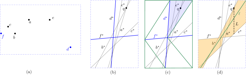
A well-known approach for finding a minimum area triangle among a set of points [8] is to use point-line duality. For each point , construct a line , which is defined as in the dual plane. Figure 2(b) illustrates a set of lines corresponding to the points of Figure 2(a). The algorithm uses the property that the line with the smallest vertical distance from the intersection point of a pair of lines and determines a triangle that minimizes the area over all the triangles that must include and . Consequently, one can first construct a line arrangement in the dual plane and then examine its faces to find a minimum area triangle in classical time.
We now describe our approach using quantum computing. One can check whether three lines in the dual plane intersect at a common point in quantum time [1], and if so, it would correspond to a triangle of 0 area. Therefore, we may assume that the lines are in a general position.
We first discuss the concept of ‘zone’ in an arrangement and some properties of a minimum area triangle. Let be an arrangement of a set of randomly chosen dual lines, and let be a triangulation obtained from in time. The zone of a line is the set of closed faces in intersected by . Figure 2(b)–(c) illustrates a scenario where two lines have been chosen to create . For each face in , denotes the dual lines (a subset of ) that bound and the dual lines that intersect the interior of . We refer to an edge of as a dual edge if it corresponds to a dual line of a point in , otherwise, we call it a supporting edge. The line determined by a supporting edge is called a supporting line. We now have the following property of a minimum area triangle.
Lemma 3.1
Let be a minimum area triangle. Let be the intersection point of and . Assume that is not a vertex of and lies interior to a face of (e.g., Figure 2(c)). Then either one of the following or both hold: (a) belongs to . (b) belongs to , where is a zone of a supporting line of .
Proof: Assume that (a) does not hold. We now show that (b) must be satisfied. Consider a vertical line segment starting from and ending on . Since minimizes the vertical distance from , no other dual edge can intersect (e.g., Figure 2(d)). Since is enclosed by and since is outside of , there must be a supporting edge on the boundary of that intersects . If the zone of the corresponding supporting line does not contain , then we can find a dual line other than that intersects , which contradicts the optimality of . Figure 2(d) illustrates the zone of , which is shaded in orange.
We now show how to leverage Theorem 2.3. Let be the faces of . We choose as the subproblems. By Lemma 2.4, the probability of a subproblem being large is bounded by . In Lemma 3.2, we show how in time, one can check whether there is a triangle of area at most such that no subproblem contains all three dual lines . Consequently, we obtain Theorem 3.3.
Lemma 3.2
A triangle that has an area of at most and spans at least two subproblems can be computed in time.
Proof: Each candidate triangle satisfies the property that the intersection point of two of its dual lines lies in some face and the third dual line does not intersect . Here the condition (b) of Lemma 3.1 must hold and it suffices to examine the zone of each supporting line of . We thus check the zones of all the supporting lines of as follows. Specifically, given an arbitrary line, its zone in an arrangement of lines can be constructed in time [20]. Let be a supporting line and let be its zone. We search over all the faces of to find a (vertex, edge) pair, i.e., , such that they lie on opposite sides of and minimize the vertical distance from to . To process a face we construct two arrays and . Here () is an array obtained by sorting the vertices on the upper (lower) envelope of using x-coordinates in time. Since is convex, for each vertex in (), we can use () to find the dual line that has the lowest vertical distance from in time. Since the number of edges in a zone is [6], the total time required for processing all the faces is at most . For supporting lines, the running time becomes .
Theorem 3.3
Given a set of points, one can determine whether there is a triangle with area at most in quantum time.
4 Finding a Unit Disk with at least Points
Let be a set of points and consider a set of unit disks, where each disk is centered at a distinct point from . Note that to solve -Points in a Disk, it suffices to check whether there is a point that hits at least disks in . However, searching for using Theorem 2.3 requires tackling some challenges. First, we need to create a problem decomposition, where the probability of obtaining a large subproblem is bounded by an allowable error probability. This requires creating a subdivision (possibly with curves) where the size of each region (corresponding to a subproblem) is . Second, we need to find a technique to check for solutions that span two or more subproblems.
Consider an arrangement of randomly chosen disks from . We first discuss how the regions of can be further divided to create a subdivision where the size of each region is .
Lemma 4.1
Let be an arrangement of unit disks. In time, one can create a subdivision of by adding straight line segments such that each face is of size .
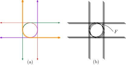
Proof: For each disk, we create four pseudolines as follows. Consider partitioning the disk into four regions by drawing a vertical and a horizontal line through its center. For each circular arc, we create a pseudoline by extending its endpoints by drawing two rays following the tangent lines, as shown in Figure 4.1(a). However, the resulting subdivision may still contain faces with linear complexity (e.g., the face in Figure 4.1(b)). We subdivide each face further by extending a horizontal line segment from each vertex. The details are included in Appendix A. At the end of the construction, each cell of the subdivision can be described using arcs or segments. The construction inserts at most straight lines and takes time per addition to complete the process in time.
We now show how to leverage Theorem 2.3. Let be the faces of . Let , where , be the disks that intersect the closed region (except its vertices), but do not fully contain . We subtract how many disks fully contain from and therefore, they should not be considered in the recursive subproblems. We show that the probability of a subproblem being large is bounded by (Appendix B). Lemma 4.2 shows how to check whether there is a solution point (i.e., a point hitting at least disks) that coincides with a vertex of or spans at least two subproblems in time. Consequently, we obtain Theorem 4.3.
Lemma 4.2
Let be a point that hits at least disks. If coincides with a vertex of or spans at least two subproblems then it can be found in time.
Proof: For each edge of , we first count the number of disks intersected by in time. We then compute all the intersection points between and the input disks and sort them based on their distances from in time. Finally, we walk along from to , and each time we hit an intersection point , we update the current disk count (based on whether we are entering a new disk or exiting a current disk) to compute the number of disks intersected by .
Theorem 4.3
Given a set of points, one can determine whether there is a unit disk with at least points in quantum time.
5 Determining Interval Containment
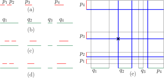
Let be an instace of Interval Containment, and let and where , be the two sets of pairwise disjoint intervals of . We now give an -time quantum algorithm to determine whether can be translated so that it becomes contained in . If there is an affirmative solution, then we can continuously move the intervals in until an endpoint of one of its intervals hits an endpoint of an interval of , as shown in Figure 3(c)–(d).
Remark 5.1
If admits an affirmative solution, then there is a solution where an end point of one interval of coincides with an end point of an interval in .
We now use Remark 5.1 to find a solution for .
Theorem 5.2
Given two sets and of pairwise-disjoint intervals on a line, one can determine whether there is a translation of that makes it contained in in quantum time.
Proof: We place the intervals of on the positive x-axis starting from and the intervals of on the positive y-axis starting from , as shown in Figures 3(e). Consider a set of horizontal lines and a set of vertical lines through the endpoints of the intervals of and , respectively. Let be an arrangement determined by randomly chosen lines from , e.g., the thick blue lines of Figures 3(e). Add the smallest area rectangle containing and to the arrangement so that we get a subdivision , where its faces are rectangles. By , where , we denote the lines of and that intersect the closed region .
We now show how to leverage Theorem 2.3. By Remark 5.1, it suffices to examine pairs of endpoints from and . Let be an endpoint from and be an endpoint from that determine a solution. Let be the intersection point of the corresponding lines and . We refer to as the solution point, which may lie at a vertex, or interior to an edge, or interior to a face of .
We choose as the subproblems. By Lemma 2.4, the probability of a subproblem being large is bounded by . In time, we can check whether coincides with a vertex of , i.e., spans at least two subproblems (Figure 3(e)). However, we do not check whether the solution lies on an edge of because if lies interior to an edge or a face of , then it is found by a Grover search over the subproblems. The running time follows directly from Theorem 2.3.
6 Pair/Tuple Search and Generalizations
For a pair search problem , if we can decide whether a given pair corresponds to a solution in classical time, then a straightforward application to Grover search yields an -time quantum algorithm. However, we show how to solve in -time even when .
Theorem 6.1
Let be a problem of size where a solution for can be defined by a pair of elements in . Assume that we can decide whether a given pair corresponds to a solution in classical time. Then a solution pair can be computed in time using a quantum algorithm.
Proof: We first label the elements of from to . For each element , we create a horizontal line and a vertical line . Every pair of lines , where one is horizontal and the other is vertical, corresponds to a pair of elements . Now the search over the subdivision is similar to the proof of Theorem 5.2.
Theorem 6.1 allows for an -time quantum algorithm for Polygon Cutting and Disjoint projections problems. The details are in Appendix C. The pair search technique can be applied to obtain quantum speed up as long as the check for a pair takes sub-quadratic time. For example, if a pair can be checked in classical time, then the analysis of Theorem 2.3 gives an algorithm with quantum time. Hence a maximum clique in a unit disk graph, where pairs of points are checked in classical time [10, 11], can be found in quantum time. The pair search technique generalizes to -tuple search, where one needs to search for a solution over an arrangement in . Appendix D includes the details.
Theorem 6.2
Let be a problem of size where a solution for can be defined by a -tuple of elements in , where . Assume that we can decide whether a given tuple corresponds to a solution in classical time, where . Then a solution for can be computed in time using a quantum algorithm.
7 Conclusion
In this paper we discuss quantum speed-up for some geometric 3SUM-Hard problems. We also show how our technique can be applied to a more general pair or tuple search setting. A natural avenue to explore would be to establish nontrivial lower bounds under quantum 3SUM conjecture.
References
- [1] A. Ambainis and N. Larka. Quantum algorithms for computational geometry problems, 2020.
- [2] B. Aronov and S. Har-Peled. On approximating the depth and related problems. SIAM J. Comput., 38(3):899–921, 2008.
- [3] G. Barequet and S. Har-Peled. Polygon containment and translational min-Hausdorff-distance between segment sets are 3sum-hard. Int. J. Comput. Geom. Appl., 11(4):465–474, 2001.
- [4] G. Brassard, P. Hoyer, M. Mosca, and A. Tapp. Quantum amplitude amplification and estimation. Contemporary Mathematics, 305:53–74, 2002.
- [5] H. Buhrman, B. Loff, S. Patro, and F. Speelman. Limits of quantum speed-ups for computational geometry and other problems: Fine-grained complexity via quantum walks. In Proc. of the 13th Innovations in Theoretical Computer Science Conference (ITCS), volume 215 of LIPIcs, pages 31:1–31:12. Schloss Dagstuhl - Leibniz-Zentrum für Informatik, 2022.
- [6] B. Chazelle, L. J. Guibas, and D.-T. Lee. The power of geometric duality. BIT Numerical Mathematics, 25(1):76–90, 1985.
- [7] K. L. Clarkson. New applications of random sampling in computational geometry. Discret. Comput. Geom., 2:195–222, 1987.
- [8] H. Edelsbrunner and L. J. Guibas. Topologically sweeping an arrangement. J. Comput. Syst. Sci., 38(1):165–194, 1989.
- [9] H. Edelsbrunner, M. Overmars, and D. Wood. Graphics in flatland: A case study. In Computational Geometry: Theory and Applications, volume 1. 1983.
- [10] D. Eppstein. Graph-theoretic solutions to computational geometry problems. In C. Paul and M. Habib, editors, Proceedings of the 35th International Workshop on Graph-Theoretic Concepts in Computer Science (WG), pages 1–16, 2009.
- [11] J. Espenant, J. M. Keil, and D. Mondal. Finding a maximum clique in a disk graph. In E. W. Chambers and J. Gudmundsson, editors, Proceedings of the 39th International Symposium on Computational Geometry (SoCG), volume 258 of LIPIcs, pages 30:1–30:17. Schloss Dagstuhl - Leibniz-Zentrum für Informatik, 2023.
- [12] A. Gajentaan and M. H. Overmars. On a class of o problems in computational geometry. Computational geometry, 5(3):165–185, 1995.
- [13] A. Gajentaan and M. H. Overmars. On a class of problems in computational geometry. Comput. Geom., 45(4):140–152, 2012.
- [14] L. K. Grover. A fast quantum mechanical algorithm for database search. In Proceedings of the twenty-eighth annual ACM symposium on Theory of computing, pages 212–219, 1996.
- [15] L. K. Grover. A framework for fast quantum mechanical algorithms. In Proceedings of the 13th Annual ACM Symposium on the Theory of Computing (STOC), pages 53–62. ACM, 1998.
- [16] D. Halperin and M. Sharir. Arrangements. In Handbook of discrete and computational geometry, pages 723–762. Chapman and Hall/CRC, 2017.
- [17] D. Haussler and E. Welzl. Epsilon-nets and simplex range queries. In Proceedings of the Second Annual ACM SIGACT/SIGGRAPH Symposium on Computational Geometry, pages 61–71. ACM, 1986.
- [18] d. B. Mark, C. Otfried, v. K. Marc, and O. Mark. Computational geometry algorithms and applications. Spinger, 2008.
- [19] E. Ruci. Cutting a Polygon with a Line. PhD thesis, Carleton University, 2008.
- [20] H. Wang. A simple algorithm for computing the zone of a line in an arrangement of lines. In Symposium on Simplicity in Algorithms (SOSA), pages 79–86. SIAM, 2022.
Appendix A Subdividing an Arrangement of Straight Line Segments and Circular Acrs
In this section, we show how to subdivide an arrangement of line segments and circular arcs in time such that the region corresponding to each cell can be described with straight line segments and circular arcs. Note that it suffices to subdivide each face of the arrangement independently, because a subproblem is determined by the subset of disks that intersect a cell, which is independent of any information regarding other cells in the arrangement. Specifically, let and be two faces in the arrangement as shown in Figure 4(a), which are subdivided with straight line segments (shown in gray). Since they are subdivided independently, the cell of does not contain the information about the vertices that are added on its boundary when is being subdivided. In other words, the cell can be described only by the two line segments that appear inside and an arc that appears on .
In the following, we show how to subdivide an -vertex face in time such that the region corresponding to each cell can be described with straight line segments and circular arcs.
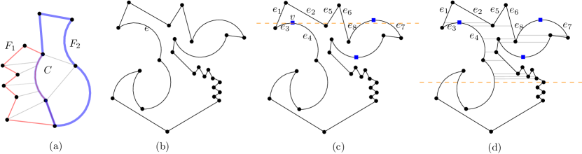
Since a straight line can be considered as an arc of a circle with an infinite radius, in the following we do not distinguish between segments and arcs. We first subdivide each arc of by adding (at most two) dummy vertices on the arc such that in the resulting face , all arcs become y-monotone. For example, the edge in Figure 4(a) is split into and , as shown in Figure 4(b). Since we need to add at most dummy vertices, this step takes time.
We sort the vertices of in decreasing order of their -coordinates. We then sweep downward with a horizontal line from the topmost vertex of . While sweeping the plane, we keep a dynamic binary search tree over the arcs that are being intersected by [18]. is updated to process the events, i.e., when we reach the bottommost or topmost endpoint of an edge, where an update operation on takes time.
Each time the sweep line hits a vertex , we examine its incident edges. We use to find the arcs and to the left and right of , respectively, which are horizontally visible to inside . For example, in Figure 4(b), the left and right edges of are and , respectively. Note that sometimes and may correspond to edges that are incident to (e.g., consider the topmost vertex of ). We examine and to determine whether the horizontal visibility lines from to these edges lie inside the face, and if so, we draw a line segment through to hit these edges.
Every time a horizontal visibility line is drawn, we obtain a new cell above this line in the subdivision. A cell cannot have any vertex on its left and right sides; otherwise, that vertex would split the cell further. Therefore, a cell can be described by two arcs bounding the left and right sides and at most two line segments bounding the top and bottom sides. Since we have update operations, the overall time complexity is .
Appendix B Computing Subproblem Size with Pseudolines
The following lemma is a generalization of Lemma 2.4.
Lemma B.1
Let be a set of simple pseudolines in , where every pair of lines intersect at most times, and let be an arrangement of pseudolines that are randomly chosen from . Let be a planar subdivision of size obtained by adding some straight line segments to such that each face of is of size . Then the probability of a closed face of , without its vertices, intersecting more than pseudolines of is bounded by , where is a positive constant and is an allowable error probability.
Proof: We adapt the proof of Ambainis and Larka [1]. Let be the chosen pseudolines. Assume that no pseudolines intersect more than times, where is a constant, and let be any straight line segment or pseudoline of . Let be the ordered intersections with pseudolines from , where . We color the intersection points corresponding to the pseudolines of white, otherwise, color them black. Define . We say a pseudo-line is bad if it has consecutive black intersections.
| number of white intersection points | |||
From Ambainis and Larka [1], this is bounded by . Since the size of is , the probability of to contain a bad pseudoline is bounded by . Let be a face of with edges where is a constant. Since does not contain any bad line, the number of pseudolines that can intersect is at most , as required.
Appendix C Polygon Cutting and Disjoint Projections
Let be an instance of Polygon Cutting. If has an affirmative solution that intersects the given edge and cuts the input polygon into pieces, then a solution can be described by a pair of vertices of as follows: First move continuously until it hits a vertex of and then continuously rotate clockwise anchored at until it hits another vertex .
If the pair is specified, then a corresponding solution (if exists) can be computed as follows. Let be the line through . Sweep to find a line parallel to that lies on one half-plane of such that no vertex of appears between and . Similarly, find another line on the other half-plane of . Considering the construction of , one of the lines among and corresponds to a solution. Given a pair , such a check can be done in time. By Theorem 6.1, we obtain a solution for Polygon Cutting in quantum time.
We can apply a similar technique for the Disjoint Projections problem, and thus obtain the following theorem.
Theorem C.1
An instance of Polygon Cutting (or, Disjoint Projections) of size can be solved in quantum time, where denotes the size of .
Appendix D Tuple Search
One can also generalize the pair search to -tuple search. In this case, we can arrange the elements of on basis vectors that are pairwise orthogonal, and search over a -dimensional arrangement.
Note that we have a set of hyperplanes, where , and it can be partitioned into subsets where the hyperplanes in each subset are parallel to each other. Let be a set of randomly chosen hyperplanes from and let be the arrangement of . Every cell of is a hypercube and thus contains faces of dimension .
We now show that the subproblem sizes would be small, i.e., no cell is intersected by hyperplanes from , where . Let , where , be a face of cell with its normal parallel to the th basis vector. If a cell is intersected by at least hyperplanes from , then a face is intersected by at least of these hyperplanes, and of these belong to some . We now show that the probability of a face being intersected by at least hyperplanes from is bounded by .
Let be such a hyperplane determined by . Since the hyperplanes of are parallel to each other and since each hyperplane of is perpendicular to , we can order these hyperplanes based on their distances from the origin. We now examine the probability of being bad, i.e., having a face intersected by at least hyperplanes of . We now apply the same analysis as we did in the proof of Lemma B.1, as follows. We can set aside consecutive hyperplanes that intersect a cell in ways, and for each option, can be chosen from the remaining hyperplanes in ways. Here the term is bounded by [1]. Note that for every , . Therefore, the probability of to be bad over all , where , is , and the probability of any of the hyperplanes of to be bad is .
We now extend the proof of Theorem 2.3 to -dimensions by setting , where the algorithm will return an error if any of the subproblems is larger than . Given a -tuple, if one can check whether it corresponds to a solution in time, where , then we obtain the following time complexity with an analysis similar to Theorem 2.3. The only exception is that the branching factor and construction time of the arrangement both increase to [16], where .
If , then . Hence . For , this is bounded by .