Unsupervised machine learning for supercooled liquids

Abstract

Unraveling the relation between structural information and the dynamic properties of supercooled liquids is one of the grand challenges of physics. Dynamic heterogeneity, characterized by the propensity of particles, is often used as a proxy for the dynamic slowing down. In this work, we introduce an unsupervised machine learning approach based on a time-lagged autoencoder (TAE) to elucidate the effect of structural features on the long-time dynamic heterogeneity of supercooled liquids. The TAE uses an autoencoder to reconstruct features at time $t+\Delta t$ from input features at time $t$ for individual particles, and the resulting latent space variables are considered as order parameters. In the Kob-Andersen system, with a $\Delta t$ about a thousand times smaller than the relaxation time, the TAE order parameter exhibits a remarkable correlation with the long-time propensity. We find that radial features on all length-scales are required to capture the long-time dynamics, consistent with recent simulations. This shows that fluctuations of structural features contain sufficient information about the long-time dynamic heterogeneity.

The glass transition is a fascinating phenomenon in physics. As a liquid is cooled, for some substances, crystallization is avoided and an amorphous solid state is reached. The static structure, for example, the powder x-ray diffraction pattern, is similar to that of a liquid, but the dynamic properties, for example, the viscosity, are slower by several orders of magnitude. Understanding the mechanism of the glass transition is one of the grand challenges in liquid state physics.

Supercooling of the liquid is accompanied by the emergence of dynamic heterogeneity: molecules in some regions exhibit active re-arrangement, while molecules in other regions are almost frozen on the time-scale of the experiment.[1] It is often suggested that the weak correlation between traditional measures of “structure” and “dynamics” can be attributed to this dynamic heterogeneity. In recent years, significant effort has been dedicated to elucidating the correlation between dynamical heterogeneity and structural properties.[2] In this work, we introduce an unsupervised machine learning method to estimate the long time dynamic heterogeneity from short simulations of the liquid.

An important advance in addressing the structural origin of dynamic heterogeneity is the concept of propensity of motion[2, 3] . The propensity is obtained from iso-configurational ensemble simulations, where a number of trajectories are obtained from the same starting configuration, but with different initial velocities. The dynamic propensity is defined as either the absolute displacement [4, 5] or the bond-breaking correlation function [6, 7] of a particle in a specified time interval, averaged over all the trajectories in the ensemble. Simulations clearly show dynamic heterogeneity, i.e., there is a distribution of propensities, with particles of similar propensities clustered spatially. The simulations do not, however, elucidate the origin of this heterogeneity.

Machine learning (ML) has become a powerful tool in computational physics, and there have been many attempts to apply these techniques to investigate the dynamic heterogeneity of supercooled liquids [8, 6, 7, 9, 10, 4, 11, 12, 13]. The majority of studies are supervised methods where the model is trained on a particular output label, e.g., the propensity. A drawback of supervised methods is that they require prior knowledge of the dynamic propensities of the training dataset, which necessitates long-time iso-configurational ensemble simulations. In addition, the large number of fit parameters necessitates a substantial amount of training data[4], making supervised methods computationally intensive. They are also not generalizable, i.e., for every new system, a new training dataset must be generated. There have been a few unsupervised ML studies (which do not require prior training with target properties), but their performance is less robust than the supervised methods[5, 14, 15, 7].

Figure 1: Schematic representation of the unsupervised machine learning method with a Time-lagged AutoEncoder (TAE). At a given temperature, the input feature vector ${\bf X}_{i}(t)$ consists of the local structure of the $i^{th}$ particle at time $t$, while the output feature vector ${\bf X}_{i}(t+\Delta t)$ consists of the same same features, for the same particle, at time $t+\Delta t$. After training, the order parameters are the values of the latent space (grey) variables.

In this work we investigate dynamic heterogeneity of supercooled liquids via unsupervised ML. The departure from previous unsupervised methods is that we use a time-lagged autoencoder (TAE)[16] (Figure. 1). The TAE is a neural network that reconstructs the structural features of each particle at time $t+\Delta t$ from its corresponding features at time $t$. The latent space variables of each particle serve as order parameters. We find that these order parameters correlate with the propensity, and therefore the width of the distribution of order parameters is a measure of the dynamic heterogeneity. Note that the training does not use any information about the target property, e.g., propensity, and it is therefore completely unsupervised.

A key parameter in the method is the lag time, $\Delta t$. If $\Delta t$=0, the TAE reduces to the autoencoder, whose order parameters show limited correlation with the long-time dynamics[5, 15]. If $\Delta t$ is large, then the method is not useful because it requires long-time simulations. We demonstrate that for small but non-zero $\Delta t$, e.g., one thousandth the relaxation time, $\tau$ (the time where self-part of intermediate scattering function decays to $1/e$ of the initial value), the TAE order parameter shows a strong correlation with the propensity at long times.

We study the 3D Kob-Andersen (KA) 80:20 binary Lennard-Jones mixture [17]. The system consists of 3277 particles of type A and 819 particles of type B, which interact via a Lennard–Jones potential: $V_{\alpha\beta}(r)=4\epsilon_{\alpha\beta}\left[\left(\frac{\sigma_{\alpha\beta}}{r}\right)^{12}-\left(\frac{\sigma_{\alpha\beta}}{r}\right)^{6}\right]$ where $\alpha,\beta\in\{A,B\}$, $\epsilon_{AA}=1.0$, $\epsilon_{AB}=1.5$, $\epsilon_{BB}=0.5$, $\sigma_{AA}=1.0$, $\sigma_{AB}=0.8$ and $\sigma_{BB}=0.88$. The units for distance, time, and temperature are $\sigma_{AA}$, $\sigma_{AA}\sqrt{m/\epsilon_{AA}}$, and $\epsilon_{AA}/k_{B}$, respectively, where $k_{B}$ is Boltzmann’s constant, and $m$ is the mass of the particles. Equilibrium configurations are obtained for reduced temperatures ranging from $0.44$ to $0.56$. Dynamic propensities are calculated from at least 30 independent isoconfigurational ensemble simulations (see the Supplemental Material (SM) for details). All results are reported for A-particles, but we note that all findings are independent of particle type. We also characterize the dynamics by the non-Gaussian parameter, $\alpha(t)\equiv\frac{3}{5}\frac{\langle(\Delta r)^{4}\rangle}{\langle(\Delta r)^{2}\rangle^{2}}-1$ where $\Delta r$ is the particle displacement at time $t$. The peak value of $\alpha$ is denoted as $\alpha_{m}$.

The first step in unsupervised ML methods is the construction of the feature vector ${\bf X}_{i}(t)$ for particle $i$ at time $t$. Following previous work[8], we employ the radial density distribution around particle $i$, which is expressed through Gaussian kernel functions: $G_{i}(r,\delta,s)=\sum_{j\neq i,s_{j}=s}e^{-\frac{(r_{ij}-r)^{2}}{2\delta^{2}}}$, where $r_{ij}$ signifies the distance between particle $i$ and its surrounding particle $j$, $s_{j}=\{A,B\}$ is the species of particle $j$. We define $r$ by considering 60 radial shells between 0.5 and 2 (in units of $\sigma_{AA}$, with $\delta=0.025$), 20 between 2 and 3 (with $\delta=0.05$), and 20 between 3 and 5 (with $\delta=0.1$). The value of $G_{i}$ in each shell of two particle types constitute a 200-dimensional vector. The $G_{i}$ vector is processed via mean-free and covariance matrix whitening is processed (see SM) to give the feature ${\bf X}_{i}$ for particle $i$. We also follow previous studies to use rotationally-invariant spherical harmonics functions to construct angular features but find that they do not provide useful information (see SM).

The TAE network (Figure 1) is constructed to map ${\bf X}_{i}(t)$(input) to ${\bf X}_{i}(t+\Delta t)$(output). Once the latent space variables are identified, we utilize principal component analysis (PCA) to orthogonalize and re-order the them, obtaining two independent order parameters denoted as $\lambda_{1}$ and $\lambda_{2}$ (details are in the SM).

Figure 2: Correlation between dynamic propensity and order parameter. (a) The Pearson correlation between bond-breaking propensity $C_{B}$ and $\lambda_{1}$, obtained from TAE with $\Delta t=$ 0.01, 0.1, and 10 for A-particles at temperature $T=0.50$. The correlation between $C_{B}$ and the order parameter from AE with $\Delta t=0$ is shown for comparison. (b) The 2-dimensional latent space in the TAE ($\Delta t=0.1$). Each point represents an individual A-particle, and the color is assigned based on the $C_{B}$ propensity. (c) Correlation between $C_{B}$ and the order parameter $\lambda_{1}$ of TAE models ($\Delta t=0.1$) constructed at different temperatures. (d) Comparison with results from supervised machine learning methods and physics-based order parameters taken from Ref. 4. In this case, the correlation is computed based on the absolute displacement propensity. The relaxation times for T=0.44, 0.47, 0.50, and 0.56, are $\tau$=4961, 77, 10, and 2, respectively.

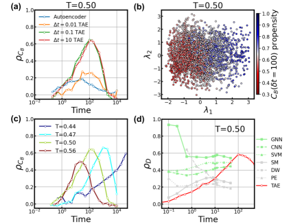
We find the latent order parameter $\lambda_{1}$ correlates well with long-time propensities from isoconfigurational simulations. Figure 2 (a) illustrates the Pearson correlation coefficient $\rho_{C_{B}}=cov(C_{B}^{i},\lambda_{1}^{i})/\sqrt{var(C_{B}^{i})var(\lambda_{1}^{i})}$ for T=0.50, where $C_{B}^{i}$ is the bond-breaking propensity of particle $i$, and $\lambda^{i}_{1}$ is the TAE order parameter of particle $i$. Even with a small lag time $\Delta t=0.1(\approx 0.01\tau)$, $\lambda_{1}$ exhibits a strong correlation with bond-breaking propensities from time $\sim\tau$ to $\sim 50\tau$. In contrast, for $\Delta t=0$ (autoencoder) or 0.01, there is only a weak correlation, and there is no difference in the correlation between $\Delta t$=0.1 and 10. This suggests that static fluctuations at fairly short times capture long-time dynamic heterogeneity. Figure 2(b) shows a map of the two order parameters where each point represents a particle color coded according to its propensity. There is a clustering of slow and fast particles, along the $\lambda_{1}$ coordinate, although the separation is not sharp. The TAE demonstrates robust performance across a wide temperature range and, the peak in the correlation coefficient occurs around the time-scale of the relaxation time of the system (Figure 2(c)). As the temperature is decreased, the TAE order parameter exhibits strong correlation with propensity over longer time scales.

The performance of the TAE is comparable to those of supervised ML models. Figure 2(d) compares the TAE to previous supervised models, including graph neural network (GNN), convolutional neural network (CNN) and support vector machine (SVM), in terms of the Pearson correlation coefficient $\rho_{D}$ between $\lambda_{1}$ and the absolute displacement propensity [4]. The TAE predictions are comparable or slightly superior to supervised models in the long-time regime. This is significant because the supervised methods are trained on the very quantity, i.e., propensity, that they attempt to predict, whereas the TAE predictions rely solely on the underlying structures. Additionally, we compare the soft modes (SM) method[3], which utilizes the mode participation fraction of each particle for the low-frequency soft normal modes, the Debye-Waller (DW) factor[18] that employs the ground-truth dynamics up to $3/4$ of the initial value of the intermediate scattering function (i.e.,corresponds to time $\approx 0.4$ for $T=0.50$), and the potential energy (PE)[19, 20] as order parameters to discern long-time dynamic heterogeneity. The TAE has a higher Pearson correlation coefficient for long-time dynamics compared to these approaches.

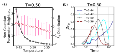
After optimizing the parameters (i.e., weights and biases) of the TAE at a specific temperature, they can be transferred to other temperatures without additional optimization. To evaluate the transferability of the TAE, we construct the network at one temperature, e.g., T=0.50, and then use this to encode features of particles from equilibrium configurations at other temperatures, thus determining the order parameter value as a function of temperature (Note that this does not require additional simulations at other temperatures, just ensembles of configurations from equilibrium simulations). At each of the other temperatures, there is a distribution of $\lambda_{1}$ due to A-particles from different configurations. Figure 3(a) shows that the TAE predicts an increase in $\lambda_{1}$ as the temperature is decreased. The increase in $\lambda_{1}$ is linear and not as dramatic and sensitive as in the case of, for example, the peak value of non-Gaussian parameter $\alpha_{m}$, shown for comparison. The values of $\lambda_{1}$ thus obtained, however, show good correlation with the propensities measured at the corresponding temperatures (Figure 3 (b)). The predictive performance of the TAE at different temperatures is comparable to that of TAE specifically constructed for those temperatures (Figure 2(c)). The TAE therefore has predictive power at temperatures different from where its parameters are determined.

Figure 3: (a) The distribution of $\lambda_{1}$ (red dots) at different temperatures encoded by a TAE constructed at $T=0.50$. The heights, $\alpha_{m}$, of the peaks of the non-Gaussian parameter (black squares) are shown for comparison. (b) Transferability of the TAE to different temperatures. The TAE is constructed at T=0.5 and used in conjunction with configurations at other temperatures to obtain $\lambda_{1}$ at that temperature. The correlation with propensities obtained at the corresponding temperature are shown.

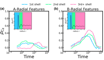
Radial features at all length-scales are important for the success of the TAE. To investigate the importance of features for dynamic prediction, we restrict the TAE (T=0.50, $\Delta t=0.1$) to features in three regions: from 0 to the first minimum in the pair correlation function, between the first and second minima, and beyond the second minimum. (Figure 4). When only the densities of surrounding A-particles are used in the feature (Figure 4(a)), the correlation with propensity is limited; however, when only the densities of surrounding B-particles are used (Figure 4(b)), the correlation with propensity is stronger. Radial features on all length-scales are required for a good correlation with the propensity; the performance of the TAE with a subset of features (Figure 4) is not as strong as when all the features are employed (Figure 2 (a)). This is consistent with a recent unsupervised ML study on the phases of water [21] and a supervised ML study on the KA model [13].

Figure 4: The radial density features subsampled based on the particle types (a) A-type and (b) B-type, and for different spatial regions. The different curves for the correlation between $\lambda_{1}$ and the propensity are obtained using features from similarly colored regions in the graph for the pair correlation function.

In summary, we introduce a fast and easily implementable unsupervised ML method to study the dynamic heterogeneity of supercooled liquids. The model identifies an order parameter, based on structural information, that correlates well with dynamic propensity. Using information from short simulations at a specific temperature to construct TAE, the order parameter can be transferred to correlate with long-term propensities at other temperatures. Importantly the TAE uses a single time lag, which is short enough to be computationally feasible and requires no information about the target property. An intriguing conclusion is that the essence of the long time dynamics is already encoded into the fluctuating structural behaviors at short times, although the “structure” is not a simple pair-based metric but rather arises from a non-linear transformation through the neural network. The results also demonstrate the utility of unsupervised ML models in the study of dynamic processes in liquids, which is currently an unexplored area of physics.

See pages 1 of SuppMatPdf/supercooled_liquid_SI.pdf See pages 2 of SuppMatPdf/supercooled_liquid_SI.pdf See pages 3 of SuppMatPdf/supercooled_liquid_SI.pdf See pages 4 of SuppMatPdf/supercooled_liquid_SI.pdf See pages 5 of SuppMatPdf/supercooled_liquid_SI.pdf See pages 6 of SuppMatPdf/supercooled_liquid_SI.pdf See pages 7 of SuppMatPdf/supercooled_liquid_SI.pdf See pages 8 of SuppMatPdf/supercooled_liquid_SI.pdf See pages 9 of SuppMatPdf/supercooled_liquid_SI.pdf See pages 10 of SuppMatPdf/supercooled_liquid_SI.pdf See pages 11 of SuppMatPdf/supercooled_liquid_SI.pdf See pages 12 of SuppMatPdf/supercooled_liquid_SI.pdf See pages 13 of SuppMatPdf/supercooled_liquid_SI.pdf See pages 14 of SuppMatPdf/supercooled_liquid_SI.pdf See pages 15 of SuppMatPdf/supercooled_liquid_SI.pdf