Estimation and Inference in Ultrahigh Dimensional Partially Linear Single-Index Models

Abstract

This paper is concerned with estimation and inference for ultrahigh dimensional partially linear single-index models. The presence of high dimensional nuisance parameter and nuisance unknown function makes the estimation and inference problem very challenging. In this paper, we first propose a profile partial penalized least squares estimator and establish the sparsity, consistency and asymptotic representation of the proposed estimator in ultrahigh dimensional setting. We then propose an $F$-type test statistic for parameters of primary interest and show that the limiting null distribution of the test statistic is $\chi^{2}$ distribution, and the test statistic can detect local alternatives, which converge to the null hypothesis at the root-$n$ rate. We further propose a new test for the specification testing problem of the nonparametric function. The test statistic is shown to be asymptotically normal. Simulation studies are conducted to examine the finite sample performance of the proposed estimators and tests. A real data example is used to illustrate the proposed procedures.

Keywords: Local alternative; penalized least squares; semiparametric regression modeling; sparsity.

1 Introduction

Thanks to advances in computing technologies, high dimensional modeling has been increasingly common in economics and finance, including microeconomics, macroeconomics, marketing, and portfolio selection as well as other areas such as medical studies and health studies. See Fan et al. (2020) for an overview. In high dimensional analysis, statistical inference has attracted considerable attention. Recently there are many developments for testing low dimensional parametric components in high dimensional models, see for instance Barber and Candès (2015), Lan et al. (2016), Ning and Liu (2017), Candès et al. (2018) Shi et al. (2019), Liu et al. (2021) and references therein. However, these works focused on high dimensional parametric modeling. It is unknown whether their works apply to more general settings, e.g. semiparametric setting.

Compared with parametric regression modeling, semiparametric models relax restrictive assumptions on parametric models and are flexible enough to capture the relationship between the response and the covariates. The partially linear single-index model (PLSIM) is one of the popular semiparametric regression models and is widely used in economics. See, for example, Example 1.1.6 in Härdle et al. (2012) for an interesting application of PLSIM.

Let $Y$ be the response, $\mathbf{X}$ and $\mathbf{Z}$ be the $p$- and $q$-dimensional covariates, respectively. In this paper, $q$ is fixed while $p$ is allowed to be exponential order of the sample size. Thus we consider the ultrahigh dimensional setting. The PLSIM is

$$Y=\eta(\bm{\alpha}^{\top}\mathbf{X})+\bm{\beta}^{\top}\mathbf{Z}+\epsilon,$$ (1.1)

where $\bm{\alpha}$ and $\bm{\beta}$ are unknown parameters, $\eta(\cdot)$ is an unknown smooth function, $E(\epsilon|\mathbf{X},\mathbf{Z})=0$, and $E(\epsilon^{2}|\mathbf{X},\mathbf{Z})=\sigma^{2}$. For model identification, assume that $\|\bm{\alpha}\|_{2}=1$ and its first element is positive, where $\|\cdot\|_{2}$ is the $L_{2}$ norm. Model (1.1) is quite general. When $p=1$, it reduces to the partially linear model (Speckman, 1988) while it turns to be the single-index model (Ichimura, 1993) when $\bm{\beta}=0$.

To estimate the parameters in model (1.1), Carroll et al. (1997) proposed a backfitting algorithm, which may lead to unstable estimators. To deal with this issue, Yu and Ruppert (2002) introduced a penalized spline estimation procedure. Xia and Härdle (2006) developed an estimator based on the minimum average variance estimation. Liang et al. (2010) proposed a profile least squares estimation procedure. Under a mild assumption that the covariate $\mathbf{Z}$ has a dimension reduction structure on the covariate $\mathbf{X}$, Wang et al. (2010) proposed a two-stage procedure. Zhu and Xue (2006) conducted confidence regions for the parameters in model (1.1) based on bias-corrected empirical likelihood. However, these works only deal with the case when dimension of $\mathbf{X}$ is small and fixed.

When the dimension of $\mathbf{X}$ is large compared with the sample size $n$, it is challenging to estimate the parameters. To handle this issue, it is natural to assume that the high dimensional nuisance parameter $\bm{\alpha}$ is sparse. In other words, only a small number of elements of $\bm{\alpha}$ are nonzero. Under this sparsity assumption, variable selection procedures are developed by many authors. See for instance, Liang et al. (2010), Zhang et al. (2013), Lai et al. (2014), and Zhang et al. (2017). However, these studies all focus on the situation that $p$ and $q$ are both fixed. As an exception, when the dimension $p+q=o(n^{1/3})$, Zhang et al. (2012) considered the estimation and variable selection problem for PLSIM. In this paper, we adopt penalty-based variable selection methods such as Tibshirani (1996) and Fan and Li (2001) to ultrahigh dimensional PLSIM. A notable feature of our approach is that we only penalize the nuisance parameter $\bm{\alpha}$, and do not penalize the parameter of interest $\bm{\beta}$.

In addition to estimation and variable selection, we are also interested in making statistical inference on the parametric component $\bm{\beta}$ and the nonparametric function $\eta(\cdot)$. That is, to test whether $H_{01}:\bm{\beta}=0$ and $H_{02}:\eta(t)=g(t,\zeta)$ with $g(\cdot,\cdot)$ being known up to an unknown parameter vector $\zeta\in\mathbb{R}^{d}$. The hypothesis $H_{01}$ is usually called significance testing problem, while the hypthesis $H_{02}$ is referred to as model-specification testing problem. When the dimension of $\mathbf{X}$ is fixed, the specification testing problem $H_{02}$ has been investigated by many authors. See for instance, Zheng (1996), Lavergne and Patilea (2012), Guo et al. (2016), and Li et al. (2016). The tests for $H_{01}$ and $H_{02}$ may be used to address the following interesting and important questions: given $\mathbf{X}$, does $\mathbf{Z}$ carry additional information about the response $Y$? Is the function form of $\eta(\cdot)$ linear or not? For these questions, when the dimensions of $\mathbf{X}$ and $\mathbf{Z}$ are fixed, Liang et al. (2010) constructed suitable test statistics based on residual sums of squares under the null and alternative hypotheses. However, the procedure developed in Liang et al. (2010) are not directly applicable for high dimensional $\mathbf{X}$. Moreover, due to the presence of nonparametric function the setting studied in this paper is distinguished from the existing works on statistical inference for the high dimensional parametric regression model. To make inference for the parameter $\bm{\beta}$ in model (1.1), we have to estimate the nuisance parameter $\bm{\alpha}$ and the nuisance function $\eta(\cdot)$. For high dimensional $\mathbf{X}$, this is very challenging. Without an appropriate estimation, high dimensional nuisance parameter $\bm{\alpha}$ and the nuisance function $\eta(\cdot)$ may significantly deteriorate the detection power of related testing methods. We show that our proposed estimators are very helpful to make suitable inference about the parametric component $\bm{\beta}$ and the nonparametric function $\eta(\cdot)$.

This work makes several interesting contributions to the literature. Firstly, we establish the asymptotic distributions of partial penalized least squares estimator for high dimensional and even ultrahigh dimensional PLSIM. Previous studies mainly focus on the finite and fixed dimension setting, while our procedure allows the dimensionality to be exponential order of the sample size and the sparsity level to be diverging. Secondly, we propose an F-type test for the parametric component $\bm{\beta}$ and show that the limiting null distribution is $\chi^{2}$ distribution. Thirdly, we study the specification testing problem for the nonparametric component $\eta(\cdot)$, propose a test statistic and show that it follows an asymptotic normal distribution.

The paper is organized as follows. In section 2, we propose the partial penalized least squares estimators and derive their asymptotic distributions. In section 3, we propose tests for the parametric component $\bm{\beta}$ and the nonparametric part $\eta(\cdot)$, and derive their asymptotical distributions. In section 4, numerical studies are conducted to illustrate the performances of our proposed test statistics. Conclusions and discussions are given in section 5. All proofs are given in the supplementary material of this paper.

2 Profile partial penalized least squares estimators

Suppose that $\{\mathbf{X}_{i},\mathbf{Z}_{i},Y_{i}\},i=1,\cdots,n$, is a sample from model (1.1). To ensure model (1.1) identifiable, we assume that $\|\bm{\alpha}\|_{2}=1$ and its first element is positive. This constraint reduces dimension of $\bm{\alpha}$ from $p$ to $p-1$. As in Yu and Ruppert (2002), Wang et al. (2010) and Cui et al. (2011), we adopt the ‘delete-one-component’ method and write $\bm{\alpha}=((1-\|\bm{\alpha}^{(1)}\|^{2}_{2})^{1/2},\bm{\alpha}^{(1)^{\top}})^{\top}$ with $\bm{\alpha}^{(1)}=(\alpha_{2},\cdots,\alpha_{p})^{\top}$. Thus $\bm{\alpha}$ can be viewed as a function of $\bm{\alpha}^{(1)}$, and the $p\times(p-1)$ Jacobian matrix is

$$J(\bm{\alpha}^{(1)})=\frac{\partial\bm{\alpha}}{\partial\bm{\alpha}^{(1)}}=\left(\begin{array}[]{c}-\dfrac{\bm{\alpha}^{(1)\top}}{(1-\|\bm{\alpha}^{(1)}\|^{2}_{2})^{1/2}}\\ I_{(p-1)\times(p-1)}\\ \end{array}\right).$$ (2.3)

Let $\bm{\theta}=(\bm{\beta}^{\top},\bm{\alpha}^{(1)\top})^{\top}$, and denote $\bm{\theta}_{0}=(\bm{\beta}^{\top}_{0},\bm{\alpha}^{(1)\top}_{0})^{\top}$ to be the true value of $\bm{\theta}$. Let $J_{0}=J(\bm{\alpha}^{(1)}_{0})$. Further denote the estimator of $\bm{\theta}$ by $\widehat{\bm{\theta}}=(\widehat{\bm{\beta}}^{\top},\widehat{\bm{\alpha}}^{(1)\top})^{\top}$, which will be specified later.

We next develop an estimation procedure for model (1.1) based on profile least squares method. Specifically, for any given $\bm{\theta}=(\bm{\beta}^{\top},\bm{\alpha}^{(1)\top})^{\top}$, we use local linear regression to estimate $\eta(\cdot)$ by minimizing

$$\sum_{i=1}^{n}[Y_{i}-\bm{\beta}^{\top}\mathbf{Z}_{i}-d_{0}-d_{1}(\bm{\alpha}^{\top}\mathbf{X}_{i}-t)]^{2}K_{h}(\bm{\alpha}^{\top}\mathbf{X}_{i}-t),$$ (2.4)

with respect to $d_{0}$ and $d_{1}$, where $K_{h}(\cdot)=K(\cdot/h)/h$ is for a kernel function $K(\cdot)$ with bandwidth $h$. Denote $(\widehat{d}_{0},\widehat{d}_{1})$ to be the minimizer of (2.4). Then for given $\bm{\theta}$, $\widehat{\eta}(t;\bm{\theta})=\widehat{d}_{0}$ and $\widehat{\eta}^{\prime}(t;\bm{\theta})=\widehat{d}_{1}$ for a specific $t$. Specifically, define

$$S_{nl}(t;\bm{\alpha}) = \frac{1}{n}\sum_{i=1}^{n}(\bm{\alpha}^{\top}\mathbf{X}_{i}-t)^{l}K_{h}(\bm{\alpha}^{\top}\mathbf{X}_{i}-t);$$

$$U_{nk}(t;\bm{\alpha}) = K_{h}(\bm{\alpha}^{\top}\mathbf{X}_{k}-t)\{S_{n2}(t;\bm{\alpha})-(\bm{\alpha}^{\top}\mathbf{X}_{k}-t)S_{n1}(t;\bm{\alpha})\};$$

$$W_{nj}(t;\bm{\alpha}) = U_{nj}(t;\bm{\alpha})/\sum_{k=1}^{n}U_{nk}(t;\bm{\alpha}).$$

Then

$$\widehat{\eta}(\bm{\alpha}^{\top}\mathbf{X}_{i},\bm{\theta})=\sum_{j=1}^{n}W_{nj}(\bm{\alpha}^{\top}\mathbf{X}_{i};\bm{\alpha})(Y_{j}-\bm{\beta}^{\top}\mathbf{Z}_{j}).$$ (2.5)

Define partial penalized least squares function as

$$Q_{n}(\bm{\theta},\lambda)=\frac{1}{2n}\sum_{i=1}^{n}\{Y_{i}-\widehat{\eta}(\bm{\alpha}^{\top}\mathbf{X}_{i},\bm{\theta})-\bm{\beta}^{\top}\mathbf{Z}_{i}\}^{2}+\sum_{j=1}^{p-1}p_{\lambda}(|\alpha^{(1)}_{j}|),$$ (2.6)

where $p_{\lambda}(\cdot)$ is a penalty function with tuning parameter $\lambda$. Minimizing (2.6) with respect to $\bm{\beta}$ and $\bm{\alpha}^{(1)}$ leads to their estimates $\widehat{\bm{\beta}}$ and $\widehat{\bm{\alpha}}^{(1)}$. It is worth noting that the nonparametric function $\eta(\cdot)$ is estimated locally, while the parametric vectors $\widehat{\bm{\beta}}$ and $\widehat{\bm{\alpha}}^{(1)}$ are obtained globally by incorporating the penalty function. It is crucial that we penalize only the nuisance parameter $\bm{\alpha}$. On one hand, it can significantly reduce the dimension of the nuisance parameter. On the other hand, it would not shrink the small elements of $\bm{\beta}$ to be zero, and thus we can construct hypothesis testing on $\bm{\beta}$ with local power.

2.1 Theoretical results

We next study the theoretical properties of the proposed estimation procedure. Assume that the penalty function $p_{\lambda}(t_{0})$ is increasing and concave in $t_{0}\in[0,\infty)$, and has a continuous derivative $p^{\prime}_{\lambda}(t_{0})$ with $p^{\prime}_{\lambda}(0+)>0$. Let $\rho(t_{0},\lambda)=p_{\lambda}(t_{0})/\lambda$ for $\lambda>0$. In addition, assume $\rho^{\prime}(t_{0},\lambda)$ is increasing in $\lambda\in(0,\infty)$ and $\rho^{\prime}(0+,\lambda)$ is independent of $\lambda$. For any vector $\mathbf{v}=(v_{1},\cdots,v_{r})^{\top}$, define

$$\bar{\rho}(\mathbf{v},\lambda)=\{\mbox{sgn}(v_{1})\rho^{\prime}(|v_{1}|,\lambda),\cdots,\mbox{sgn}(v_{r})\rho^{\prime}(|v_{r}|,\lambda)\}^{\top},$$

where $\mbox{sgn}(v_{1})=I(v_{1}>0)-I(v_{1}<0)$. Following Fan and Lv (2011a), we further define the local concavity of the penalty function $\rho$ at $\mathbf{v}$ as

$$\kappa(\rho,\mathbf{v},\lambda)=\lim_{\epsilon\rightarrow 0^{+}}\max_{1\leq j\leq r}\sup_{t_{1}<t_{2}\in(|v_{j}|-\epsilon,|v_{j}|+\epsilon)}-\frac{\rho^{\prime}(t_{2},\lambda)-\rho^{\prime}(t_{1},\lambda)}{t_{2}-t_{1}}.$$

Before we proceed further, let us introduce some notations. Denote $\mathcal{A}=\{j:\alpha^{(1)}_{0,j}\neq 0\}$ and $s=|\mathcal{A}|$ be the number of elements in $\mathcal{A}$. Define $\mathcal{A}^{c}=[1,\cdots,p-1]-\mathcal{A}$ be the complement set of $\mathcal{A}$. Let $\bm{\alpha}^{(1)}_{\mathcal{A}}$ be the subvector of $\bm{\alpha}^{(1)}$ formed by elements in $\mathcal{A}$. Similarly let $B_{{\mathcal{A}}}$ be the submatrix of a matrix $B$ formed by columns in ${\mathcal{A}}$. Moreover $\bm{\vartheta}=(\bm{\beta}^{\top},\bm{\alpha}^{(1)\top}_{\mathcal{A}})^{\top}$, and $\bm{\vartheta}_{0},\widehat{\bm{\vartheta}}$ are similarly defined. Further let $J_{\mathcal{A}}$ be the submatrix of $J$ formed as follows

$$J_{\mathcal{A}}(\bm{\alpha}^{(1)}_{\mathcal{A}})=\left(\begin{array}[]{c}-\dfrac{\bm{\alpha}^{(1)\top}_{\mathcal{A}}}{(1-\|\bm{\alpha}^{(1)}_{\mathcal{A}}\|^{2}_{2})^{1/2}}\\ I_{s\times s}\\ \end{array}\right).$$

$J_{0,\mathcal{A}}=J_{\mathcal{A}}(\bm{\alpha}^{(1)}_{0,\mathcal{A}})$. Let $l_{n}=\min_{j\in\mathcal{A}}|\alpha^{(1)}_{0,j}|/2$, the half minimum signal of $\bm{\alpha}^{(1)}_{0,\mathcal{A}}$. Define $\mathcal{N}_{0}=\{\bm{\theta}\in\mathbb{R}^{p+q-1}:\|\bm{\vartheta}-\bm{\vartheta}_{0}\|_{2}\leq l_{n}\}$. Let $\Gamma_{i0}=\bm{\alpha}_{0}^{\top}\mathbf{X}_{i},\Gamma_{i1}=\bm{\alpha}^{\top}\mathbf{X}_{i},\eta_{i0}=\eta(\Gamma_{i0})$, and $\eta_{i1}=\eta(\Gamma_{i1})$. Further let ${\mathcal{A}}^{*}={\mathcal{A}}\cup\{1\},\mu_{1}(\Gamma_{i1})=E[\mathbf{X}_{i,{\mathcal{A}}^{*}}|\Gamma_{i1}],\widetilde{\mathbf{X}}_{i}(\bm{\alpha})=\mathbf{X}_{i,{\mathcal{A}}^{*}}-\mu_{1}(\Gamma_{i1}),\mu_{2}(\Gamma_{i1})=E[\mathbf{Z}_{i}|\Gamma_{i1}]$, $\widetilde{\mathbf{Z}}_{i}(\bm{\alpha})=\mathbf{Z}_{i}-\mu_{2}(\Gamma_{i1})$, $\mu^{\star}_{1i}=\mu_{1}(\Gamma_{i0}),\mu^{\star}_{2i}=\mu_{2}(\Gamma_{i0}),\widetilde{\mathbf{X}}^{\star}_{i}=\widetilde{\mathbf{X}}_{i}(\bm{\alpha}_{0}),$ $\widetilde{\mathbf{Z}}^{\star}_{i}=\widetilde{\mathbf{Z}}_{i}(\bm{\alpha}_{0})$, and $c_{n}=O(h^{2}+\sqrt{\log n/nh^{3}})$. Define $L_{i}=\left(\begin{array}[]{c}\widetilde{\mathbf{Z}}_{i}^{\star}\\ \eta_{i0}^{\prime}J_{0,\mathcal{A}}^{\top}{\mathbf{X}}_{i}^{\star}\end{array}\right)$, $\Sigma^{\star}=E[L_{i}L_{i}^{T}].$ For a vector $\mathbf{v},\|\mathbf{v}\|_{\infty}=\max|v_{i}|$. For matrix $B$, denote $\lambda_{\min}(B)$ and $\lambda_{\max}(B)$ to be the minimum and maximum eigenvalues of the matrix $B$. $\|B\|_{2,\infty}=\sup_{\bm{v}:\|\bm{v}\|_{2}=1}\|B\bm{v}\|_{\infty}$. Throughout the paper, $c$ and $C$ are two generic positive constants.

We impose the following conditions:

• $\lambda_{\min}(\Sigma^{\star})\geq c>0$, $\lambda_{\max}(\Sigma^{\star})=O(1)$. For any $1\leq i\leq n,1\leq j\leq p$, $X_{ij}$ are uniformly bounded.

• $l_{n}\gg\lambda_{n}\gg\max\{n^{1/\varpi+\varsigma}c_{n},n^{1/\varpi+\varsigma}\sqrt{s/n},\sqrt{\log p/n}\}$ with some $\varpi\geq 8$ and some arbitrary small $\varsigma>0$, $p^{\prime}_{\lambda_{n}}(l_{n})=o((ns)^{-1/2})$, $\lambda_{n}\kappa_{0}=o(1)$ where $\kappa_{0}=\max_{\bm{\delta}\in\mathcal{N}_{0}}\kappa(\rho,\bm{\delta},\lambda_{n})$. Here $a\gg b$ means $\lim_{n\rightarrow\infty}a/b=\infty$.

• Assume that $E(|\epsilon_{i}|^{\varpi})\leq C$ and ${\log p}/{n^{1-2/\varpi-\varsigma}}\rightarrow 0$. For any $\bm{\alpha}$ with $\|\bm{\alpha}-\bm{\alpha}_{0}\|_{2}=O(\sqrt{s/n})$, let $R_{ki}=(J^{\top}(\mathbf{X}_{i}-E[\mathbf{X}_{i}|\mathbf{X}^{\top}_{i}\bm{\alpha}]))_{k}\eta^{\prime}_{i1}$. Let $\mathbf{R}=(R_{ki})_{i=1,\cdots,n}^{k=1,\cdots,p}$ and $\tilde{\mathbf{Z}}(\bm{\alpha})=(\tilde{\mathbf{Z}}_{1}(\bm{\alpha}),\cdots,\tilde{\mathbf{Z}}_{n}(\bm{\alpha}))$. Assume that

  $$\|\mathbf{R}^{T}_{\mathcal{A}^{c}}(\tilde{\mathbf{Z}}(\bm{\alpha}),\mathbf{R}_{\mathcal{A}})\|_{2,\infty}=O_{p}(n^{1+1/\varpi+\varsigma}),\,\,\,\max_{1\leq l\leq q}\sup_{\bm{\theta}\in\mathcal{N}_{0}}E[\tilde{Z}_{l}^{4}(\bm{\alpha})|\Gamma_{i1}]<C<\infty.$$

  $E(L_{1}^{T}L_{1}|\Gamma_{10}=\gamma)/s$ is bounded uniformly for $\gamma$.

• $\eta(\cdot)$ is twice order continuously differentiable on its support $\mathcal{D}$. $\eta^{\prime}(\cdot)$ and $\eta^{\prime\prime}(\cdot)$ are bounded on $\mathcal{D}$. For any $\bm{\alpha}$ with $\|\bm{\alpha}-\bm{\alpha}_{0}\|_{2}=O(\sqrt{s/n})$, the density function of $\bm{\alpha}^{\top}\mathbf{X}$, $f(x)$ is bounded away from 0 on $\mathcal{D}$. $\sup_{x}f(x)\leq B_{0}<\infty$. For some $q>0,\delta>0$ and $M>2$, $E|\Gamma_{i1}|^{2q+\delta}<\infty$. If $T_{ik}$ is one of the following: $X_{ik},X_{ik}\eta_{i1},X_{ik}\eta^{\prime}_{i1},$

  $$\sup_{k\in\mathcal{A}}\sup_{x}E(|T_{1k}|^{M}|\Gamma_{11}=x)f(x)\leq B_{1}<\infty,$$

  $$\sup_{k\in\mathcal{A}}\sup_{x}|x|^{q}E(T_{1k}|\Gamma_{11}=x)f(x)\leq B_{2}<\infty.$$

  First order derivatives of $f(x)\mu_{1i}(x),f(x)\mu_{2j},f(x)\mu_{1i}(x)\eta(x),f(x)\eta(x)$ exist and are L-Lipschitz, and $\eta^{\prime}(x)\mu_{1i}(x),\mu_{2j}(x)$ are L-Lipschitz, where $\mu_{1i}(x)$, $\mu_{2j}(x)$ are the $i$th and $j$th components of $\mu_{1}(x)$, $\mu_{2}(x)$ respectively, $i\in\mathcal{A}^{\star}$, $1\leq j\leq q$, $0<L<\infty$.

• Suppose $K(u)$ is a differentiable and symmetric kernel function and $G(u)$ is one of the following: $K(u),tK(u),t^{2}K(u),tK^{\prime}(u),t^{2}K^{\prime}(u)$. $G(u)$ is satisfying that $|G^{\prime}(u)|\leq\lambda_{1}<\infty$. When $|u|>L$, $|G^{\prime}(u)|\leq\lambda_{1}|x|^{-\eta}$, $|G(u)|\leq\lambda_{2}|u|^{-q}\leq\bar{G}<\infty$ for some $\eta>1$, $L>0$ and $\lambda_{2}<\infty$. $\int|G^{2}(u)|du<\infty.$ $\int u^{4}|G^{2}(u)|du<\infty.$

• Assume that $s=o(n^{1/2})$, $h\log n\rightarrow 0$, $nh^{8}\rightarrow 0$, $nh^{3}/(s\log n)\rightarrow\infty,$ and
  $nh^{4}/(\log n)^{2}\rightarrow\infty$.

• Assume that $s=o(n^{1/3}),s^{3}h^{4}\rightarrow 0,sh\log n\rightarrow 0,nsh^{8}\rightarrow 0,$ $nh^{3}/(s^{3}\log n)\rightarrow\infty,$ and $nh^{4}/(s(\log n)^{2})\rightarrow\infty$.

These conditions are mild and commonly assumed. The uniform boundedness of elements of covariate $\mathbf{X}$ in condition (A1) is usually assumed to facilitate the technical arguments, see for instance Wang et al. (2010) and Sherwood and Wang (2016). But for $\mathbf{Z}$, uniform boundedness is not required. The effect of nonparametric estimation is taken into account in Condition (A2). The rates of $l_{n}$ and $\lambda_{n}$ are required for sparsity. In condition (A2), a minimum signal assumption is imposed on the nuisance parameter $\bm{\alpha}$. This is required for variable selection consistency and evaluation of the uncertainty of the estimation for small signals. However, we should emphasize that no minimum signal condition is imposed on $\bm{\beta}$, the parameter of primary interest. Thus, we can still detect local alternative hypotheses effectively. This condition is reasonable in many practical applications. Van de Geer et al. (2014) and Ning and Liu (2017) do not impose such conditions. However, some additional assumptions are imposed. In fact, the validity of the decorrelated score statistic depends on the sparsity of additional parameter $\mathbf{w}^{*}$. From Remark 6 in Ning and Liu (2017), we know that for testing univariate parameters of high dimensional linear regression model, this requires the degree of a particular node in the graph to be relatively small when the covariate follows a Gaussian graphical model. A further discussion about the decorrelated score statistic is given in Remark 1. From Conditions (A2) and (A3), clearly the dimensionality $p$ is allowed to be exponential order of the sample size $n$. In the theory of high dimensional regression, Gaussian or sub-Gaussian tail condition for the random error $\epsilon$ is usually assumed. However, in this paper, we only require a very mild moment condition. Condition (A4) is some regularity conditions for uniform convergence for kernel estimation and for the smoothness of related functions. Condition (A5) is the usual condition for the kernel function $K(\cdot)$ and is satisfied when $K(\cdot)$ is the density of normal distribution or a smooth density function with compact support.

Condition (A6a) is required to control the estimation error due to nonparametric estimators, while (A6b) is stronger and needed for asymptotic representation of $\widehat{\bm{\theta}}$. If we set $s$ to be fixed, then conditions (A6a) and (A6b) reduce to be $nh^{3}/\log n\rightarrow\infty,nh^{4}/(\log n)^{2}\rightarrow\infty,nh^{8}\rightarrow 0$ and $h\log n\rightarrow 0$, which are assumed by many authors for partially linear single-index model with fixed dimension. Thus conditions (A6a) and (A6b) are modifications of classical conditions to accounting for the effect of $s$. Take $h=O(n^{-c_{1}}),s=O(n^{c_{2}}),1/8<c_{1}<1/4,0\leq c_{2}<1/2$, then conditions in (A6a) are satisfied when $1-3c_{1}-c_{2}>0$. This leads to $c_{2}<1-3c_{1}.$ If we set $c_{1}=1/5$, we can get $0\leq c_{2}<2/5$. For condition (A6b), it requires that

$$c_{2}<1/3,\,\,c_{2}<c_{1},\,\,1+c_{2}-8c_{1}<0,\,\,1-3c_{1}-3c_{2}>0,1-4c_{1}-c_{2}>0.$$

These lead to

$$c_{2}<\min\{\frac{1}{3},c_{1},8c_{1}-1,\frac{1}{3}-c_{1},1-4c_{1}\}.$$

If we set $c_{1}=1/5$, the condition is satisfied provided that $0\leq c_{2}<2/15$.

We first establish the rate of convergence of $\widehat{\bm{\alpha}}$ and its sparsity, and then derive an asymptotic representation of $\widehat{\bm{\vartheta}}$ in the following theorem.

Theorem 1.

Under Conditions (A1)-(A6a), the following holds. With probability tending to 1, $\widehat{\bm{\alpha}}^{(1)}$ must satisfy (i) $\widehat{\bm{\alpha}}^{(1)}_{\mathcal{A}^{c}}=0$. (ii) $\|\widehat{\bm{\alpha}}^{(1)}_{\mathcal{A}}-\bm{\alpha}^{(1)}_{0,\mathcal{A}}\|_{2}=O_{p}(\sqrt{s/n})$. If further condition (A6b) holds, we obtain that

$$\sqrt{n}(\widehat{\bm{\vartheta}}-\bm{\vartheta}_{0}) = \Sigma^{\star-1}\frac{1}{\sqrt{n}}\sum_{i=1}^{n}\epsilon_{i}\left(\begin{array}[]{ccc}\widetilde{\mathbf{Z}}^{\star}_{i}\\ \eta^{\prime}_{i0}J^{\top}_{0,\mathcal{A}}\widetilde{\mathbf{X}}_{i}^{\star}\\ \end{array}\right)+o_{p}(1).$$ (2.9)

The proof of this theorem is given in the supplementary material of this paper. Theorem 1 establishes the sparsity, consistency and asymptotic representation of the proposed profile partial penalized least squares estimators. Our results allow the dimensionality $p$ to be exponential order of the sample size $n$. The sparsity level $s$ is also allowed to be diverging. Theorem 1 implies that the optimal bandwidth $h=O(n^{-1/5})$ may be used for not only the sparsity and consistency, but also for the asymptotic representation, and $s$ may be of order $o(n^{2/5})$ for the sparsity and consistency. However, for the asymptotic representation, more restrictive conditions on $h$ and $s$ as in condition (A6b) are required.

3 Hypothesis testing

This section aims for developing hypothesis testing procedures for both $\bm{\beta}$ and $\eta(\cdot)$.

3.1 Testing the parametric component

Of interest is to test hypothesis

$$H_{01}:\bm{\beta}=0\quad\mbox{versus}\quad H_{11}:\bm{\beta}\neq 0.$$ (3.1)

Under $H_{11}$, the residual sum of squares is

$$\mbox{RSS}_{1}=\sum_{i=1}^{n}[Y_{i}-\widehat{\eta}(\widehat{\bm{\alpha}}^{\top}\mathbf{X}_{i},\widehat{\bm{\theta}})-\widehat{\bm{\beta}}^{\top}\mathbf{Z}_{i}]^{2}.$$ (3.2)

Under $H_{01}$, we need to consider the constrained penalized least squares estimators. Specially, for any given $\bm{\theta}=(\widetilde{\bm{\beta}}^{\top},\bm{\alpha}^{(1)\top})^{\top}$ with $\widetilde{\bm{\beta}}=0$, we first obtain the constrained profile estimator for the nonparametric function:

$$\widetilde{\eta}(\bm{\alpha}^{\top}\mathbf{X}_{i},\bm{\theta})=\sum_{j=1}^{n}W_{nj}(\bm{\alpha}^{\top}\mathbf{X}_{i};\bm{\alpha})Y_{j}.$$ (3.3)

Denote the constrained penalized least squares function as

$$\widetilde{Q}_{n}(\bm{\theta},\lambda)=\frac{1}{2n}\sum_{i=1}^{n}[Y_{i}-\widetilde{\eta}(\bm{\alpha}^{\top}\mathbf{X}_{i},\bm{\theta})]^{2}+\sum_{j=1}^{p-1}p_{\lambda}(|\alpha^{(1)}_{j}|),$$ (3.4)

for some penalty function $p_{\lambda}(\cdot)$ with a tuning parameter $\lambda$. Minimizing the above objective function with respect to $\bm{\alpha}^{(1)}$ leads to the estimator $\widetilde{\bm{\alpha}}^{(1)}$. Afterwards, we define the residual sum of squares $RSS_{0}$ under the null hypothesis:

$$\mbox{RSS}_{0}=\sum_{i=1}^{n}[Y_{i}-\widetilde{\eta}(\widetilde{\bm{\alpha}}^{\top}\mathbf{X}_{i},\widetilde{\bm{\theta}})]^{2}.$$ (3.5)

Here $\widetilde{\bm{\theta}}=(0^{\top},\widetilde{\bm{\alpha}}^{(1)\top})^{\top}$. Under the null hypothesis, $RSS_{0}$ and $RSS_{1}$ should be close, while under the alternative hypothesis, $RSS_{0}$ should be larger than $RSS_{1}$. This motivates us to consider the following test statistic:

$$T_{n}=\frac{RSS_{0}-RSS_{1}}{RSS_{1}/(n-q)}.$$ (3.6)

We impose the following condition.

• Assume that $\|\bm{\delta}_{n}\|_{2}=O(\sqrt{1/n})$. Here $\bm{\delta}_{n}$ corresponds to local alternative hypotheses $H_{11}^{(n)}:\bm{\beta}=\bm{\delta}_{n}$.

Theorem 2.

Suppose that Conditions (A1)-(A7) hold, then we have

$$\sup_{x}|P(T_{n}\leq x)-P(\chi^{2}_{q}(n\bm{\delta}_{n}^{\top}\Phi^{-1}\bm{\delta}_{n}/\sigma^{2})\leq x)|\rightarrow 0.$$ (3.7)

where $\Phi=(I_{q},0_{q\times s})\Sigma^{\star-1}(I_{q},0_{q\times s})^{\top}$ and $\chi^{2}_{q}(n\bm{\delta}_{n}^{\top}\Phi^{-1}\bm{\delta}_{n}/\sigma^{2})$ is a noncentral chi-square random variable with $q$ degrees of freedom and noncentrality parameter $n\bm{\delta}_{n}^{\top}\Phi^{-1}\bm{\delta}_{n}/\sigma^{2}$ which is allowed to vary with $n$.

The proof of Theorem 2 is given in the supplementary material of this paper. From Theorem 2, it is clear that the null distribution of $T_{n}$ is a chi-square random variable with $q$ degrees of freedom, which does not depend on nuisance parameter $\bm{\alpha}$ nor the nuisance function $\eta(\cdot)$. This implies that the so-called Wilks phenomenon still holds even in the (ultra)high dimensional partially linear single-index model. Further, the test statistic $T_{n}$ can detect local alternatives, which converge to the null hypothesis at the root-$n$ rate.

Remark 1.

In a case that the minimum signal assumption in (A2) is believed to be invalid, we may want to extend the decorrelated score statistic to make inference about $\bm{\beta}$. However, this is not straightforward. For high dimensional partially linear single index models, the negative Gaussian quasi-loglikelihood (i.e., the least squares loss) is

$$l(\bm{\beta},\bm{\alpha})=\frac{1}{n}\sum_{i=1}^{n}[Y_{i}-\bm{\beta}^{\top}\mathbf{Z}_{i}-\eta(\bm{\alpha}^{\top}\mathbf{X}_{i})]^{2}.$$

By adopting the notations in Ning and Liu (2017), we may consider the score functions $\nabla_{\bm{\beta}}l(\bm{\beta},\bm{\alpha})=n^{-1}\sum_{i=1}^{n}[Y_{i}-\bm{\beta}^{\top}\mathbf{Z}_{i}-\eta(\bm{\alpha}^{\top}\mathbf{X}_{i})]\mathbf{Z}_{i}$ and $\nabla_{\bm{\alpha}}l(\bm{\beta},\bm{\alpha})=n^{-1}\sum_{i=1}^{n}[Y_{i}-\bm{\beta}^{\top}\mathbf{Z}_{i}-\eta(\bm{\alpha}^{\top}\mathbf{X}_{i})]\eta^{\prime}(\bm{\alpha}^{\top}\mathbf{X}_{i})J(\bm{\alpha}^{(1)})^{\top}\mathbf{X}_{i}$. When the dimension of $\mathbf{X}$ is high, we cannot directly use $\nabla_{\bm{\beta}}l(\bm{\beta},\bm{\alpha})$ to make inference for the parameter of interest $\bm{\beta}$. Instead we let

$$S(\bm{\beta},\bm{\alpha})=\nabla_{\bm{\beta}}l(\bm{\beta},\bm{\alpha})-\mathbf{W}^{\top}\nabla_{\bm{\alpha}}l(\bm{\beta},\bm{\alpha}).$$

Here $\mathbf{W}^{\top}=E[\nabla_{\bm{\beta}}l(\bm{\beta},\bm{\alpha})\nabla^{\top}_{\bm{\alpha}}l(\bm{\beta},\bm{\alpha})]E[\nabla_{\bm{\alpha}}l(\bm{\beta},\bm{\alpha})\nabla^{\top}_{\bm{\alpha}}l(\bm{\beta},\bm{\alpha})]^{-1}\in\mathbb{R}^{q\times(p-1)}$. Immediately, it follows that $E[S(\bm{\beta},\bm{\alpha})\nabla^{\top}_{\bm{\alpha}}l(\bm{\beta},\bm{\alpha})]=0$. That is, $S(\bm{\beta},\bm{\alpha})$ is uncorrelated with $\nabla_{\bm{\alpha}}l(\bm{\beta},\bm{\alpha})$. We then regard $S(\bm{\beta},\bm{\alpha})$ as the decorrelated score function for $\bm{\beta}$. The key idea is to apply a high dimensional projection of the score function of the interested parameter to the nuisance parameter space.

To make inference about $\bm{\beta}$ based on $S(\bm{\beta},\bm{\alpha})$, we need to estimate the nuisance parameter $\bm{\alpha}$, the unknown matrix $\mathbf{W}$ and the unknown functions $\eta(\cdot)$ and $\eta^{\prime}(\cdot)$. For $\bm{\alpha}$, $\eta(\cdot),\eta^{\prime}(\cdot)$ and $J(\bm{\alpha}^{(1)})$, we may adopt the partial penalized least squares estimators introduced in this paper. While for the estimator of $\mathbf{W}$, we can consider the following formula:

$$\widehat{\mathbf{W}}=\arg\min_{\mathbf{W}}\frac{1}{2n}\sum_{i=1}^{n}\|\nabla_{\bm{\beta}}l(\widehat{\bm{\theta}})-\mathbf{W}^{\top}\nabla_{\bm{\alpha}}l(\widehat{\bm{\theta}})\|^{2}_{2}+p_{\lambda^{\prime}}(\mathbf{W}),$$

for some penalty function $p_{\lambda^{\prime}}(\cdot)$ with tuning parameter $\lambda^{\prime}$. Besides the sparsity of $\bm{\alpha}$, we also require $\mathbf{W}$ to be sparse. The estimated de-correlated score function is:

$$\widehat{S}(0,\widehat{\bm{\alpha}})=\nabla_{\bm{\beta}}l(0,\widehat{\bm{\alpha}})-\widehat{\mathbf{W}}^{\top}\nabla_{\bm{\alpha}}l(0,\widehat{\bm{\alpha}}).$$

To prove the asymptotic normality of $\widehat{S}(0,\widehat{\bm{\alpha}})$, it is required to check the assumptions 3.1-3.4 in Ning and Liu (2017). Due to the complicated formula of $\widehat{S}(0,\widehat{\bm{\alpha}})$, these four assumptions are not easy to verify. The investigation of the asymptotic behavior of the decorrelated score statistic is beyond the scope of this work.

3.2 Testing the nonparametric component

In practice, it is of interest in testing whether the nonparametric function $\eta(\cdot)$ is in a specific form, for example linear, or not, or even whether it is constant. This motivates us to consider the following null hypothesis

$$H_{02}:\eta(t)\equiv g(t,\zeta)\quad\mbox{versus}\quad H_{12}:\eta(t)\neq g(t,\zeta)\ \mbox{for\ some}\ t,$$

where the form $g(\cdot,\cdot)$ is known, and $\zeta\in\mathbb{R}^{d}$ with $d$ being fixed is an unknown parametric vector. For example, if we set $g(t,\zeta)=c$, a constant, then $H_{02}$ corresponds to testing whether the predictor $\mathbf{X}$ contributes to the response $Y$ or not. When the dimension of $\mathbf{X}$ is fixed, this kind of specification testing problem has been investigated by many authors. See for instance, Zheng (1996), Guo et al. (2016), and Li et al. (2016).

Let $\epsilon_{0i}=Y_{i}-\bm{\beta}^{\top}_{0}\mathbf{Z}_{i}-g(\bm{\alpha}^{\top}_{0}\mathbf{X}_{i},\zeta_{0})=\eta(\bm{\alpha}^{\top}_{0}\mathbf{X}_{i})-g(\bm{\alpha}^{\top}_{0}\mathbf{X}_{i},\zeta_{0})+\epsilon_{i}$. Then it follows that $E(\epsilon_{0i}|\bm{\alpha}^{\top}_{0}\mathbf{X}_{i})=\eta(\bm{\alpha}^{\top}_{0}\mathbf{X}_{i})-g(\bm{\alpha}^{\top}_{0}\mathbf{X}_{i},\zeta_{0})$. Clearly, under $H_{02}$, $E(\epsilon_{0i}|\bm{\alpha}^{\top}_{0}\mathbf{X}_{i})=0$, while under $H_{12}$, it is not equal to zero. Further we have under $H_{02}$, $E[\epsilon_{0i}E(\epsilon_{0i}|\bm{\alpha}^{\top}_{0}\mathbf{X}_{i})f(\bm{\alpha}^{\top}_{0}\mathbf{X}_{i})]=0$, while under $H_{12}$, we have

$$E[\epsilon_{0i}E(\epsilon_{0i}|\bm{\alpha}^{\top}_{0}\mathbf{X}_{i})f(\bm{\alpha}^{\top}_{0}\mathbf{X}_{i})]\neq 0.$$

This motivates us to propose the following test statistic

$$S_{n}=\frac{1}{n(n-1)}\sum_{i=1}^{n}\sum_{j\neq i}^{n}\widehat{\epsilon}_{0i}\widehat{\epsilon}_{0j}\frac{1}{b}G(\frac{\widehat{\bm{\alpha}}^{\top}(\mathbf{X}_{i}-\mathbf{X}_{j})}{b}),$$ (3.8)

where $G(\cdot)$ is a kernel function, $b$ is the bandwidth, $\widehat{\epsilon}_{0i}=Y_{i}-\widehat{\bm{\beta}}^{\top}\mathbf{Z}_{i}-g(\widehat{\bm{\alpha}}^{\top}\mathbf{X}_{i},\widehat{\zeta})$, $\widehat{\bm{\beta}},\widehat{\bm{\alpha}}$ are the partial penalized least squares estimators defined in section 2, and $\widehat{\zeta}$ is the nonlinear least squares estimator obtained by minimizing

$$\min_{\zeta}\frac{1}{n}\sum_{i=1}^{n}[Y_{i}-\widehat{\bm{\beta}}^{\top}\mathbf{Z}_{i}-g(\widehat{\bm{\alpha}}^{\top}\mathbf{X}_{i},\zeta)]^{2}.$$

Denote

$$\sigma^{2}_{S}=2\int G^{2}(t)dt\cdot\int\sigma^{4}f^{2}(\bm{\alpha}^{\top}_{0}\mathbf{X})d(\bm{\alpha}^{\top}_{0}\mathbf{X});$$

$$\widehat{\sigma}^{2}_{S}=\frac{2}{n(n-1)}\sum_{i=1}^{n}\sum_{j\neq i}^{n}\frac{1}{b}G^{2}(\frac{\widehat{\bm{\alpha}}^{\top}(\mathbf{X}_{i}-\mathbf{X}_{j})}{b})\widehat{\epsilon}^{2}_{0i}\widehat{\epsilon}^{2}_{0j};$$

$$g_{01}(\cdot,\zeta_{0})=\partial g(\cdot,\zeta)/\partial\zeta|_{\zeta=\zeta_{0}};$$

$$g_{k0}(\bm{\alpha}^{\top}_{0}\mathbf{X}_{i},\cdot)=\partial^{k}g(\bm{\alpha}^{\top}\mathbf{X}_{i},\cdot)/\partial^{k}(\bm{\alpha}^{\top}\mathbf{X}_{i})|_{\bm{\alpha}=\bm{\alpha}_{0}},k=1,2;$$

$$\mathbf{N}_{i}=(\mathbf{Z}_{i}^{\top},g_{10}(\bm{\alpha}^{\top}_{0}\mathbf{X}_{i},\zeta_{0})\mathbf{X}^{\top}_{i,\mathcal{A}})^{\top};\,\,\,\mathbf{M}_{i}=(\mathbf{N}^{\top}_{i},g^{\top}_{01}(\bm{\alpha}^{\top}_{0}\mathbf{X}_{i},\zeta_{0}))^{\top}.$$

The following conditions are needed to facilitate the technical proofs.

• The kernel function $G(\cdot)$ is univariate bounded, continuous and symmetric density function satisfying $\int t^{2}G(t)dt<\infty$, and $\int|t|^{j}G(t)dt<\infty$ for $j=1,2,3$. The second order derivative of $G(\cdot)$ is bounded.

• $\lambda_{\max}(E[\mathbf{M}_{i}\mathbf{M}^{\top}_{i}])<\infty$.

• $g_{20}(\bm{\alpha}^{\top}\mathbf{X}_{i},\cdot)$ is bounded and $g_{01}(\bm{\alpha}^{\top}\mathbf{X}_{i},\zeta_{0})$ satisfies the first order Lipschitz condition for $\bm{\alpha}^{\top}\mathbf{X}_{i}$ in a neighborhood of $\bm{\alpha}^{\top}_{0}\mathbf{X}_{i}$. Further assume that $E[g^{2}_{01}(\bm{\alpha}^{\top}_{0}\mathbf{X}_{i},\zeta_{0})]<\infty$.

We then have the asymptotic normality of the proposed test statistic.

Theorem 3.

Suppose that Conditions (A1)-(A6a) and (B1)-(B3) hold, under $H_{02}$ with conditions $nb^{2}/s^{2}\rightarrow\infty$ and $sb^{1/2}\rightarrow 0$, we obtain that

$$nb^{1/2}S_{n}\rightarrow N(0,\sigma^{2}_{S}).$$ (3.9)

From the proof of Theorem 3 given in the supplementary material, we can find that it is not necessary to assume homoscedasticity in order to derive the asymptotic distribution of $S_{n}$. In fact, even under heteroscedasticity, it can be obtained that $\|\widehat{\bm{\alpha}}-\bm{\alpha}\|_{2}=O_{p}(\sqrt{s/n})$. This may further induce the results in Theorem 3. If $s$ is set to be fixed, the conditions about the bandwidth $b$ boil down to $nb^{2}\rightarrow\infty$ and $b\rightarrow 0$, which are very mild. On the other hand, if $s$ also diverges, restrictions are necessary. That is, we need $s=o(\min\{b^{-1/2},(nb^{2})^{1/2}\})$.

We now standardize $S_{n}$ to obtain a scale-invariant statistic:

$$V_{n}=\sqrt{\dfrac{n-1}{n}}\dfrac{nb^{1/2}S_{n}}{\sqrt{\widehat{\sigma}^{2}_{S}}}.$$

Corollary 1.

Suppose that Conditions (A1)-(A6a) and (B1-B3) hold, under the null hypothesis with conditions $nb^{2}/s^{2}\rightarrow\infty$ and $sb^{1/2}\rightarrow 0$, we obtain that

$$V^{2}_{n}\rightarrow\chi^{2}_{1}.$$ (3.10)

Here $\chi^{2}_{1}$ is the chi-square distribution with one degree of freedom.

3.3 Practical implementation issues

In practice, it is desirable to have a data-driven method to choose the tuning parameter $\lambda$. We modify the high-dimensional BIC-type (HBIC) criterion proposed by Wang et al. (2013) to select $\lambda$ by minimizing

$$\text{HBIC}(\lambda)=\log(\widehat{\sigma}^{2}_{\lambda})+|\mathcal{A}_{\lambda}|\dfrac{C_{n}\log p}{n},$$

where $\mathcal{A}_{\lambda}=\{j:\widehat{\alpha}_{j}^{(1)}\neq 0\}$ is the model identified by minimizing (2.6),

$$\widehat{\sigma}_{\lambda}^{2}=\dfrac{1}{n}\sum_{i=1}^{n}\left[Y_{i}-\widehat{\eta}\left(\widehat{\bm{\alpha}}^{\top}\mathbf{X}_{i},\widehat{\bm{\theta}}\right)-\widehat{\bm{\beta}}^{\top}\mathbf{Z}_{i}\right]^{2},$$

and $C_{n}$ is a sequence of numbers that should diverge to $\infty$ slowly. Wang et al. (2013) suggested setting $C_{n}=\log(\log n)$. This works well in a variety of settings in this paper.

We next discuss how to make minimization of (2.6) and (3.4) faster by using local linear approximation. Minimization problems of (2.6) and (3.4) are similar, so we only work on (2.6) as an example. To minimize (2.6), noticing that a local linear approximation of $\widehat{\eta}\left(\breve{\bm{\alpha}}^{\top}\mathbf{X}_{i},\breve{\bm{\theta}}\right)$ is

$$\widehat{\eta}(\breve{\bm{\alpha}}^{\top}\mathbf{X}_{i},\bm{\breve{\theta}})\approx\widehat{\eta}(\bm{\alpha}^{\top}\mathbf{X}_{i},\bm{\theta})+\left.\frac{\partial\widehat{\eta}(\bm{\alpha}^{\top}\mathbf{X}_{i},\bm{\theta})}{\partial\left(\bm{\alpha}^{(1)\top},\bm{\beta}^{\top}\right)}\right|_{(\bm{\alpha}^{(1)},\bm{\beta})}\left(\begin{array}[]{c}{\breve{\bm{\alpha}}^{(1)}-\bm{\alpha}^{(1)}}\\ {\breve{\bm{\beta}}-\bm{\beta}}\end{array}\right).$$

$Q_{n}(\breve{\bm{\theta}},\lambda)$ can be approximated by

$$Q_{n}(\breve{\bm{\theta}},\lambda)\approx Q^{L}_{n}(\breve{\bm{\theta}},\bm{\theta},\lambda):=\frac{1}{2n}\sum_{i=1}^{n}\left(Y_{i}^{*}-\mathbf{Z}_{i}^{*\top}\breve{\bm{\theta}}\right)^{2}+\sum_{j=1}^{p-1}p_{\lambda}\left(|\breve{\alpha}_{j}^{(1)}|\right),$$ (3.11)

where

$$Y_{i}^{*}=Y_{i}-\widehat{\eta}\left(\bm{\alpha}^{\top}\mathbf{X}_{i},\bm{\theta}\right)+\left.\frac{\partial\widehat{\eta}(\bm{\alpha}^{\top}\mathbf{X}_{i},\bm{\theta})}{\partial\left(\bm{\alpha}^{(1)\top},\bm{\beta}^{\top}\right)}\right|_{\left(\bm{\alpha}^{(1)},\bm{\beta}\right)}\left(\begin{array}[]{c}{\bm{\alpha}^{(1)}}\\ {\bm{\beta}}\end{array}\right),$$

and

$$\mathbf{Z}_{i}^{*}=\left\{\left.\frac{\partial\widehat{\eta}(\bm{\alpha}^{\top}\mathbf{X}_{i},\bm{\theta})}{\partial\left(\bm{\alpha}^{(1)\top},\bm{\beta}^{\top}\right)}\right|_{\left(\bm{\alpha}^{(1)},\bm{\beta}\right)}\right\}^{\top}+\left(\begin{array}[]{c}\bm{0}_{(p-1)\times 1}\\ {\mathbf{Z}_{i}}\end{array}\right).$$

We can solve (2.6) by iteratively minimizing penalized least squares functions. Specifically, we could take the LASSO estimate for the whole model as the initial value $\bm{\theta}^{0}$: For $k=1,2,...,$ we iteratively solve (3.12) until the sequence of $\{\bm{\theta}^{k}\}$ converges. Our numerical study shows that the algorithm can converge very fast even if the initial value is not taken close to the true value.

$$\bm{\theta}^{k+1}=\arg\min_{\bm{\theta}}Q^{L}_{n}(\bm{\theta},\bm{\theta}^{k},\lambda).$$ (3.12)

Zou and Li (2008) proposed an algorithm for maximizing the penalized likelihood for concave penalty functions based on local linear approximation (LLA). Here we may apply local linear approximation to the penalty term in (3.11),

$$p_{\lambda}\left(|\breve{\alpha}^{(1)}_{j}|\right)\approx p_{\lambda}\left(|\alpha^{(1)}_{j}|\right)+p_{\lambda}^{\prime}\left(|\alpha_{j}^{(1)}|\right)\left(|\breve{\alpha}_{j}^{(1)}|-|\alpha_{j}^{(1)}|\right),\text{ for }\breve{\alpha}^{(1)}_{j}\approx\alpha^{(1)}_{j}.$$ (3.13)

Plugging (3.13) into (3.11) with constant terms omitted, we have

$$Q^{P}_{n}(\breve{\bm{\theta}},\bm{\theta},\lambda)=\frac{1}{2n}\sum_{i=1}^{n}\left(Y_{i}^{*}-\mathbf{Z}_{i}^{*\top}\breve{\bm{\theta}}\right)^{2}+\sum_{j=1}^{p-1}p^{\prime}_{\lambda}(|\alpha_{j}^{(1)}|)(|\breve{\alpha}^{(1)}_{j}|).$$ (3.14)

The minimization problem (3.12) becomes

$$\bm{\theta}^{k+1}=\arg\min_{\bm{\theta}}Q^{P}_{n}(\bm{\theta},\bm{\theta}^{k},\lambda).$$ (3.15)

In that way, we transform the original problem into iteratively solving penalized least squares with $L_{1}$ penalty. There are effective algorithms for solving (3.15) because dealing with $L_{1}$ penalty can take advantage of kinds of computationally efficient algorithms for the LASSO, such as the least angle regression (LARS) algorithm proposed by Efron et al. (2004).

4 Numerical studies

4.1 Simulation studies

In this section, we conduct simulation studies to assess the finite-sample performance of the proposed estimation and testing methods. The SCAD penalty function (Fan and Li, 2001) is adopted in our simulation study. We also compare the proposed estimator and tests with the oracle estimator and oracle tests, where the true signal set $\mathcal{A}=\{j:\alpha^{(1)}_{0,j}\neq 0\}$ is assumed to be known and models are fitted based on that. Denote $T^{O}_{n}$ and $V^{O}_{n}$ to be the oracle test statistics. We report the performances of the profile partial penalized least squares estimator and different test statistics based on 500 replications. The sample size is taken to be 200. All simulations were conducted using MATLAB code.

Example 1. To evaluate the performance of the proposed profile partial penalized least squares estimator and F-type test statistic $T_{n}$, we generate simulation data from the following models.

Model 1a. $Y=\exp(\bm{\alpha}^{\top}\mathbf{X})+\bm{\beta}^{\top}\mathbf{Z}+\epsilon$,

Model 1b. $Y=\sin(\dfrac{\pi}{2}\bm{\alpha}^{\top}\mathbf{X})+\bm{\beta}^{\top}\mathbf{Z}+0.5\epsilon$.

For both models, we take the dimension of $\bm{\beta}$ to be $2$ and generate $\epsilon$ from $N(0,1)$. In model 1a, the coefficient $\bm{\alpha}$ for the mean function is $(\alpha_{1},\alpha_{2},\alpha_{10})^{\top}=(2,1,1)/\sqrt{6}$ and $\alpha_{j}=0$ when $j\neq 1,2,10$. We generate $\mathbf{X}=(X_{1},X_{2},\dots,X_{p})^{\top}$ and $\mathbf{Z}=(Z_{1},Z_{2})^{\top}$ from multivariate normal distributions with zero mean and covariance matrix $\bm{\Sigma}_{\mathbf{X}}=\left(\sigma_{ij}\right)_{p\times p}$ and $\bm{\Sigma}_{\mathbf{Z}}=\left(\sigma_{ij}\right)_{2\times 2}$ respectively, with $\sigma_{ij}=0.25^{|i-j|}$. We consider two scenarios for the dimension of $\mathbf{X}$, $p$: (i) $p=300$; (ii) $p=1500$. This is used to investigate the impact of dimensionality $p$. In model 1b, we set $(\alpha_{1},\alpha_{2},\alpha_{10})^{\top}=(1,1,1)/\sqrt{3}$ and $\alpha_{j}=0$ when $j\neq 1,2,10$. To evaluate the influence of correlation among covariates, three scenarios for model 1b are considered. In scenarios (i) and (ii), $\mathbf{X}$ and $\mathbf{Z}$ are generated in the same way as in model 1a, but now we take $p=1000$, $\sigma_{ij}=\rho^{|i-j|}$, and consider (i) $\rho=0.25$ and (ii) $\rho=0.75$. In scenario (iii), $\mathbf{X}$ and $\mathbf{Z}$ are correlated. We generate $\bm{V}=(V_{1},V_{2},\dots,V_{p+2})^{\top}$ from normal distribution with zero mean and covariance matrix $\bm{\Sigma}_{V}=\left(\sigma_{ij}\right)_{(p+2)\times(p+2)}$ with $\sigma_{ij}=0.75^{|i-j|}$. We let $\mathbf{Z}=(Z_{1},Z_{2})^{\top}=(V_{3},V_{4})^{\top}$, $\mathbf{X}=(X_{1},X_{2},X_{3}\dots,X_{p})^{\top}=(V_{1},V_{2},V_{5},\dots,V_{p+2})^{\top}$. In real data analysis in Section 4.2, we use 10-fold cross-validation to choose the bandwidth. But this is too time-consuming in simulation. As an alternative, we generated several data sets to get an idea about the range of an appropriate bandwidth. In simulation study of model 1a, we set the bandwidth $h=0.37$. Note that the standard error of $\bm{\alpha}^{\top}\mathbf{X}$ is 1.08 in this simulation setting. So 95% values of $\bm{\alpha}^{\top}\mathbf{X}$ lies between $-2.1$ to 2.1. This implies that for a given $t_{0}$, we estimate $\eta(t_{0})$ based on about 9 percent of observations. Similarly in model 1b, the bandwidth $h$ is set to be $0.37,0.44,0.44$ for each scenario so that we use about 9 percent of data to estimate $\eta(t_{0})$ for a given $t_{0}$.

We first examine the finite sample performance of the proposed estimators. Table LABEL:est reports the ratio of the true nonzero coefficients correctly set to nonzero, denoted by ‘T’ in the table, the ratio of the true zero coefficients incorrectly set to nonzero, denoted by ‘F’, bias and mean squared error of the resulting estimates over the 500 replications for both models under different scenarios and $\bm{\beta}=c_{1}\mathbf{1}_{2}$. In model 1a, two scenarios share the same oracle model. The ratio of the true nonzero coefficient that were correctly set to nonzero is always close to 1 and the ratio of the truly zero coefficients that are incorrectly set to nonzero is always close to 0, indicating that our method can always correctly identify the true submodel. Compared with the oracle estimator, both bias and mean squared error of $\widehat{\bm{\beta}}$ behave similar to the oracle one. Bias and mean squared error of $\widehat{\bm{\alpha}}$ is usually a little bit larger than oracle setting. The error mainly comes from the partial penalization on $\bm{\alpha}^{(1)}$ using the SCAD penalty and also from the limitation of finite sample and imperfect selection of tuning parameter $\lambda$. However, the error is in a reasonable order and is acceptable. We find from the empirical size and power for (4.1) below that the small error does not affect much statistical inference on parameters of interest.

Further we consider the following null and alternative hypotheses:

$$H_{01}:\bm{\beta}=0\text{\ \ versus\ \ }H_{11}:\bm{\beta}=c_{1}\mathbf{1}_{2}.$$ (4.1)

where $c_{1}=0,0.01,\cdots,0.05,0.1,0.15,\cdots,0.5$ for model 1a and $c_{1}=0,0.01,\cdots,0.05,\\ 0.1,0.15,0.2.$ for model 1b. When $c_{1}=0$, it corresponds to $H_{01}$, thus we can examine Type I error rate. When $c_{1}\neq 0$, it corresponds to the alternative hypothesis, which allows us to examine the power of the proposed test.

Figure 1 depicts the empirical sizes and powers of the tests under model 1a. As expected, $T_{n}$ controls the size well and is powerful since it performs as well as the oracle test $T^{O}_{n}$. The empirical power of $T_{n}$ remains roughly the same when $p$ increases from 300 to 1500. This implies that the dimension of $\mathbf{X}$ does not have a dramatic impact on the performance of $T_{n}$.

Figure 1: Empirical sizes and powers of $T_{n}$ and $T^{O}_{n}$ at significance level $0.05$ over 500 replications under model 1a. The horizontal dotted line represents level of $0.05$. The solid line, the long-dashed line, and the dashed-dotted line represent the sizes and powers of $T^{O}_{n}$, $T_{n}$ with $p=300$ and $T_{n}$ with $p=1500$, respectively

Table 1: Empirical sizes and powers of tests $T_{n}$ and $T^{O}_{n}$ under model 1b

	$c_{1}$	0	0.01	0.02	0.03	0.04	0.05	0.10	0.15	0.20
(i)	$T^{O}_{n}$	0.042	0.080	0.118	0.192	0.360	0.466	0.980	1	1
	$T_{n}$	0.058	0.086	0.109	0.266	0.343	0.506	0.937	1	1
(ii)	$T^{O}_{n}$	0.058	0.078	0.150	0.286	0.442	0.656	0.998	1	1
	$T_{n}$	0.042	0.068	0.116	0.196	0.406	0.604	0.994	1	1
(iii)	$T^{O}_{n}$	0.048	0.060	0.122	0.194	0.312	0.428	0.998	1	1
	$T_{n}$	0.052	0.076	0.125	0.188	0.296	0.436	0.960	1	1

Empirical sizes and powers of tests under model 1b are demonstrated in Table 1, from which it can be seen clearly that the empirical sizes of $T_{n}$ are close to the nominal level 0.05. Furthermore, the powers of $T_{n}$ and $T^{O}_{n}$ are close. When the covariance matrix structure changes with $\rho$ increasing from 0.25 to 0.75, the powers of $T_{n}$ and $T^{O}_{n}$ increase. This implies that covariance matrix of covariates has some impact on powers of $T_{n}$ and $T^{O}_{n}$. When $\mathbf{X}$ and $\mathbf{Z}$ are correlated, there is little power loss. In summary, the proposed test $T_{n}$ performs as well as the oracle test $T^{O}_{n}$ in terms of power, and controls the empirical sizes very well.

Example 2. This example is designed to study the performance of the nonparametric component test statistic $V_{n}$. To this end, we generate data from

Model 2. $Y=\eta(\bm{\alpha}^{\top}\mathbf{X})+0.5Z_{1}-0.3Z_{2}+0.75\epsilon$.

In this example, $\mathbf{X}$ and $\mathbf{Z}$ are generated in the same way as in model 1.a. The dimension of $\mathbf{X}$, $p$ is chosen to be 1500 here. We consider hypotheses:

$$H_{0}:\eta(t)=\zeta t\quad\text{ versus }\quad H_{1}:\eta(t)=c_{2}\sin\{\pi(t-a)/(b-a)\}+\zeta t,$$

where $c_{2}=0,0.01,\cdots,0.05,0.1,0.15,\cdots,0.5$, $a$ and $b$ are chosen to be 1.3409 and 0.3912 respectively. This model setting was used by Liang et al. (2010) with fixed $p$. True value of $\zeta$ is chosen to be 1. Again, when $c_{2}=0$, the null hypothesis is true, while if $c_{2}\neq 0$, the alternative hypothesis holds.

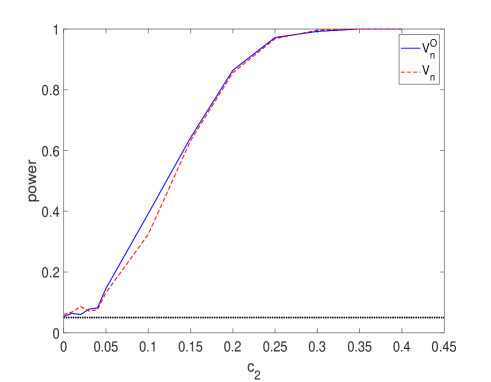
Figure 2: Empirical sizes and powers of $V_{n}$ and $V^{O}_{n}$ at the significance level $0.05$ over 500 replications under model 2. The horizontal dotted line represents the level $\alpha=0.05$. The solid line and the longdashed line represent the sizes and powers of $V^{O}_{n}$ and $V_{n}$, respectively

Figure 2 depicts the empirical sizes and powers of $V_{n}$ and $V^{O}_{n}$ at significance level 0.05. Figure 2 indicates that the empirical size of $V_{n}$ is close to the level 0.05. The empirical power of $V_{n}$ is greater than 0.95 when $c_{2}$ is greater than 0.30. Further, the empirical power of $V_{n}$ is very close to that of the oracle test $V^{O}_{n}$.

4.2 A real data example

We now illustrate the proposed methodology by an application to the supermarket data set (Wang, 2009). The data consists of $n=464$ daily records in a supermarket. Each record corresponds to the number of customers as the response and sale amount of 6398 products as predictors. We standardize both response and predictors to be with zero mean and unit variance. We fit a partially linear single-index model to the data set and aim to locate products whose sale volumes are mostly correlated with the number of customers, and perform related hypothesis testings to the regression function.

We carry out a preprocessing step that we reduce the dimension of predictors to 1000 by employing the feature screening scheme in Li et al. (2012). To decide which variables belong to the linear part $\bm{\beta}^{\top}\mathbf{Z}$ or the nonlinear part $\eta(\bm{\alpha}^{\top}\mathbf{X})$, we adopt the strategy suggested by Xia et al. (1999) and Zhang et al. (2012). Their ideas are based on dealing with the scatterplot of each variable versus the response. To take both linear behavior and goodness of fit into account, we first compute the Pearson correlation between the response $Y$ and each variable and select variables with an absolute value of the correlation greater than 0.3. Then we fit the response $Y$ and each covariate with local linear smoothing. We obtain the estimated mean function and corresponding pointwise confidence band by computing the mean plus and minus $k$ times the estimated standard deviation function. We also fit a linear regression. If the linear straight line lies in the confidence band, the variable goes into the linear part of our model. In this example, we choose $k=0.3$ as the threshold. Otherwise, if the correlation is smaller than 0.3 or the linear regression line cannot be encompassed by the confidence band, the variable goes into the single-index part. This leads to a number of 994 variables ($\mathbf{X}$) for single-index component and 6 variables ($\mathbf{Z}$) for the linear component. Model 3 below is fitted. We use 10-fold cross-validation to choose the bandwidth and HBIC to choose $\lambda$. This leads to the selected bandwidth $h=0.59$ and the selected tuning parameter $\lambda=0.12$. The fit of the semiparametric part of the model is shown in Figure 3. There are in total of 12 active variables selected from covariates $\mathbf{X}$.

Model 3. $Y=\eta({\alpha}^{\top}\mathbf{X})+\bm{\beta}^{\top}\mathbf{Z}+\epsilon.$

From Figure 3, there seems to exist a nonlinear pattern for the relationship between $\mathbf{X}$ and the response $Y$.

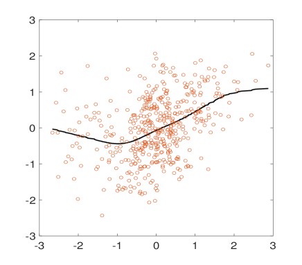
Figure 3: Scatter plot of $\widehat{\bm{\alpha}}^{\top}\mathbf{X}$ versus $Y-\widehat{\bm{\beta}}^{\top}\mathbf{Z}$. Solid line is the estimate $\widehat{\eta}(\widehat{\bm{\alpha}}^{\top}\mathbf{X},\widehat{\bm{\theta}})$ of $\eta({\bm{\alpha}}^{\top}\mathbf{X})$

We apply the proposed hypothesis testing procedures for this data set. We first consider the following two testing problems: $H_{01}:\bm{\beta}=0$ and $H_{02}:\eta(t)=c$, where $c$ is a constant. These two hypotheses $H_{01}$ and $H_{02}$ aim to test whether the covariates $\mathbf{Z}$ and $\mathbf{X}$ contribute to the response $Y$ or not, respectively. Based on the proposed test statistics $T_{n}$ and $V_{n}$, the $p$-values of the two hypotheses are 0. This implies that the selected variables indeed show a significant influence on the response. Then we further test whether the contribution of the single-index components $\mathbf{X}$ to the response $Y$ is linear or not and perform hypothesis testing $H_{03}:\eta(t)=\zeta t$. The corresponding $p$-value is 0.004. Therefore, we reject the null hypothesis that the link function for single-index part is linear at level 0.05. This is consistent with our observation on the fitting plot of the semiparametric part shown in Figure 3. In conclusion, we find there is a significant effect of the selected variables and potential non-linear relationship between selected variables and the response. It is worth pointing out that Liu et al. (2016) and Lan et al. (2016) did the analysis on the same data set but fitted high dimensional linear model on it. However, from our analysis, we find evidence that the linear model is not suitable and recommend fitting a semiparametric model on this data and data with similar attributes.

5 Conclusions and discussions

In this paper, we developed new statistical inference procedures for high dimensional partially linear single-index model. Different from linear regression model, we have to deal with the nuisance unknown function. To derive powerful hypothesis tests, we first propose a profile penalized least squares estimator and study its asymptotic properties. Then we propose an F-type test for the parametric component. We further study the specification testing problem for the nonparametric component and propose a test statistic with an asymptotic normal distribution. A notable feature is that the optimal rate for the bandwidth is allowed, even the covariate $\mathbf{X}$ is of high dimensional. No under-smoothing or over-smoothing is required. The dimensionality is allowed to be exponential order of the sample size and the sparsity level can also be diverging.

In this paper, we focus on testing the low dimensional parametric vector $\bm{\beta}$, while regard the high dimensional parametric vector $\bm{\alpha}$ as nuisance parameter. In practice, it may also be interesting to make inference on components of $\bm{\alpha}$. This issue was studied recently by Eftekhari et al. (2021) for single index model under elliptical symmetry assumption on the covariates. The extension of their procedure to PLSIM without elliptical assumption would be an interesting topic for future research.

Supplement

The supplementary material consists of three technical lemmas, the proofs of these three lemmas and proofs of all theorems in this paper.

Appendix: Technical Proofs

The following three lemmas will be used in the proofs for the main theorems, and their proofs are given in the supplementary material of this paper.

We first establish some results on uniform convergence for kernel estimation, which has been considered in several authors (Mack and Silverman, 1982; Liebscher, 1996; Hansen, 2008), but none of them considered estimating several regression functions simultaneously with the number of regression functions growing with $n$. Thus, their results cannot be directly applied for nonparametric estimation in the presence of high dimensional covariates. In Lemma A.1 below, we establish the uniform convergence rate for kernel estimation for the regression functions when the number of regression functions grows with sample size $n$. Let $X_{0}$ and $\mathbf{Y}_{0}$ be a $1$- and $s$-dimensional continuous random vector, respectively. With a slight abuse of notation, here $X_{0}$ and $\mathbf{Y}_{0}$ represent general random variable and vector, respectively, and are not the covariate and the response in the main text.

Lemma A.1.

Suppose that $\{\{X_{i},\mathbf{Y}_{i}\},i=1,\cdots,n\}$ is a random sample from $\{X_{0},\mathbf{Y}_{0}\}$, where the dimension of $\mathbf{Y}_{0}=(Y_{01},\cdots,Y_{0s})^{\top}$ grows with $n$. Let $K(\cdot)$ be a kernel function, and

$$\bm{H}(x)=\dfrac{1}{nh}\sum_{i=1}^{n}K\left(\dfrac{X_{i}-x}{h}\right)\mathbf{Y}_{i}.$$

It follows that

$$\sup_{x}\|\bm{H}(x)-E\bm{H}(x)\|_{2}=O_{p}\left(\left\{\frac{s\log n}{nh}\right\}^{1/2}\right)$$ (A.1)

under the following three assumptions:

Assumption 1. The density of $X_{0}$, $f(x)$, satisfies that $\sup_{x}f(x)\leq B_{0}<\infty$. For some $M>2$ and $q>0,\delta>0,$ $E|X_{0}|^{2q+\delta}<\infty$, and

$$\sup_{1\leq k\leq s}\sup_{x}E(|Y_{0k}|^{M}|X_{0}=x)f(x)\leq B_{1}<\infty,$$

$$\sup_{1\leq k\leq s}\sup_{x}|x|^{q}E(Y_{0k}|X_{0}=x)f(x)\leq B_{2}<\infty.$$

Assumption 2. $K(u)$ is differentiable and $\int|K^{2}(u)|<\infty$. $|K^{\prime}(u)|\leq\lambda_{1}<\infty$. There exist some constants $\eta>1$, $L>0$ and $\lambda_{2}<\infty$ such that $|K^{\prime}(u)|\leq\lambda_{1}|u|^{-\eta}$, $|K(u)|\leq\lambda_{2}|u|^{-q}\leq\bar{K}<\infty$ for $|u|>L$.

Assumption 3. The bandwidth satisfies $h\rightarrow 0$ and $s(\log n)^{1+\delta}/(n^{1-2/M}h)\rightarrow 0$ for some $\delta>0$.

We introduce some notation for the following. Let $\Gamma_{i0}=\bm{\alpha}_{0}^{\top}\mathbf{X}_{i}$, $\Gamma_{i1}=\bm{\alpha}^{\top}\mathbf{X}_{i},\eta_{i0}=\eta(\Gamma_{i0}),\eta_{i1}=\eta(\Gamma_{i1}),\widehat{\eta}_{i0}=\widehat{\eta}(\Gamma_{i0},\bm{\theta}_{0})$ and $\widehat{\eta}_{i1}=\widehat{\eta}(\Gamma_{i1},\bm{\theta})$. Further let $W_{0ij}=W_{nj}(\Gamma_{i0};\bm{\alpha}_{0})$ and $W_{1ij}=W_{nj}(\Gamma_{i1};\bm{\alpha})$. Denote $\mu_{1}(\Gamma_{i1})=E[\mathbf{X}_{i,{\mathcal{A}}^{*}}|\Gamma_{i1}],\widetilde{\mathbf{X}}_{i}(\bm{\alpha})=\mathbf{X}_{i,{\mathcal{A}}^{*}}-\mu_{1}(\Gamma_{i1}),\mu_{2i}(\Gamma_{i1})=E[\mathbf{Z}_{i}|\Gamma_{i1}]$, $\widetilde{\mathbf{Z}}_{i}(\bm{\alpha})=\mathbf{Z}_{i}-\mu_{2}(\Gamma_{i1})$, $\mu^{\star}_{1i}=\mu_{1}(\Gamma_{i0}),\mu^{\star}_{2i}=\mu_{2}(\Gamma_{i0}),\widetilde{\mathbf{X}}^{\star}_{i}=\widetilde{\mathbf{X}}_{i}(\bm{\alpha}_{0}),$ $\widetilde{\mathbf{Z}}^{\star}_{i}=\widetilde{\mathbf{Z}}_{i}(\bm{\alpha}_{0})$. Define

$$L_{i}=\left(\begin{array}[]{c}\widetilde{\mathbf{Z}}_{i}^{\star}\\ \eta^{\prime}_{i0}J^{\top}_{0,\mathcal{A}}\widetilde{\mathbf{X}}_{i}^{\star}\\ \end{array}\right);\,\,\,\widehat{L}_{i}=\left(\begin{array}[]{ccc}\mathbf{Z}_{i}+\dfrac{\partial\widehat{\eta}_{i1}}{\partial\bm{\beta}}\\ \dfrac{\partial\widehat{\eta}_{i1}}{\partial\bm{\alpha}^{(1)}_{\mathcal{A}}}\\ \end{array}\right).$$

Lemma A.2.

Under conditions (A1), (A4) and (A5), for any $\bm{\theta}$ which satisfies $\bm{\alpha}^{(1)}_{{\mathcal{A}}^{c}}=0$ and $\|\bm{\vartheta}-\bm{\vartheta}_{0}\|_{2}=O(\sqrt{s/n})$, it follows that

$$(\widehat{\eta}_{i0}-\eta_{i0})^{2}=O_{p}(h^{4}+\frac{\log n}{nh});\,\,\,\|\widehat{L}_{i}-L_{i}\|^{2}_{2}=O_{p}(s(h^{4}+\frac{\log n}{{nh^{3}}}))$$

uniformly for $i$.

Lemma A.3.

Under conditions (A1), (A4), (B2) and (B3), for any $\bm{\theta}$ which satisfies $\bm{\alpha}_{{\mathcal{A}}^{c}}=0$ and $\|\bm{\theta}-\bm{\theta}_{0}\|_{2}=O(\sqrt{s/n})$, we have:

$$\|\widehat{\zeta}-\zeta_{0}\|_{2}=O_{p}(\sqrt{\frac{s}{n}}).$$

Proof of Theorem 1:

To enhance the readability, we divide the proof of Theorem 1 into three steps. In the first step, we show that there exists a local minimizer $\bar{\bm{\theta}}$ of $Q_{n}(\bm{\theta})$ with the constraints $\bar{\bm{\alpha}}^{(1)}_{\mathcal{A}^{c}}=0$, such that $\|\bar{\bm{\theta}}-\bm{\theta}_{0}\|_{2}=O_{p}(\sqrt{s/n})$. In the second step, we prove that $\bar{\bm{\theta}}$ is indeed a local minimizer of $Q_{n}(\bm{\theta})$. This implies $\widehat{\bm{\theta}}=\bar{\bm{\theta}}$. In the final step, we derive the asymptotic expansion of $\widehat{\bm{\theta}}$.

Step 1: Consistency in the $(s+q)$-dimensional subspace: We first constrain $Q_{n}(\bm{\theta})$ on the $(s+q)$-dimensional subspace of $\{\bm{\theta}\in\mathbb{R}^{p+q-1}:\bm{\alpha}^{(1)}_{\mathcal{A}^{c}}=0\}$ of $\mathbb{R}^{p+q-1}$. This partial penalized least squares function is given by

$$\bar{Q}_{n}(\bm{\vartheta})=\frac{1}{2n}\sum_{i=1}^{n}[Y_{i}-\widehat{\eta}(\bm{\alpha}^{\top}_{{\mathcal{A}}^{*}}\mathbf{X}_{i,{\mathcal{A}}^{*}},\bm{\vartheta})-\bm{\beta}^{\top}\mathbf{Z}_{i}]^{2}+\sum_{j=1}^{s}p_{\lambda}(|\delta_{j}|).$$

Here $\bm{\vartheta}=(\bm{\beta}^{\top},\bm{\delta}^{\top})^{\top}$ and $\bm{\delta}=(\delta_{1},\cdots,\delta_{s})^{\top}$. We now show that there exists a strict local minimizer $\bar{\bm{\vartheta}}$ of $\bar{Q}_{n}(\bm{\vartheta})$ such that $\|\bar{\bm{\vartheta}}-\bm{\vartheta}_{0}\|_{2}=O_{p}(\sqrt{s/n})$. To this end, we consider an event

$$H_{n}=\{\min_{\bm{\vartheta}\in\partial\mathcal{N}_{\tau}}\bar{Q}_{n}(\bm{\vartheta})>\bar{Q}_{n}(\bm{\vartheta}_{0})\}.$$

where $\mathcal{N}_{\tau}=\{\bm{\vartheta}\in\mathbb{R}^{s+q}:\bm{\vartheta}=\bm{\vartheta}_{0}+d_{n}\bm{u},\|\bm{u}\|_{2}\leq\tau\}$ with $d_{n}=\sqrt{s/n}$, $\tau\in(0,\infty)$, and $\partial\mathcal{N}_{\tau}$ denotes the boundary of the closed set $\mathcal{N}_{\tau}$. Clearly, on the event $H_{n}$, there exists a local minimizer of $\bar{Q}_{n}(\bm{\vartheta})$ in $\mathcal{N}_{\tau}$. Thus, we only need to show that $P(H_{n})\rightarrow 1$ as $n\rightarrow\infty$ when $\tau$ is large. To this end, we next study the behavior of $\bar{Q}_{n}$ on the boundary $\partial\mathcal{N}_{\tau}$.

Define

$$D_{n}=\frac{1}{n}\sum_{i=1}^{n}[Y_{i}-\widehat{\eta}_{i1}-\bm{\beta}^{\top}\mathbf{Z}_{i}]^{2}-\frac{1}{n}\sum_{i=1}^{n}[Y_{i}-\widehat{\eta}_{i0}-\bm{\beta}^{\top}_{0}\mathbf{Z}_{i}]^{2}.$$ (A.3)

Note that

$$D_{n} = \frac{1}{n}\sum_{i=1}^{n}[\widehat{\eta}_{i1}-\widehat{\eta}_{i0}+(\bm{\beta}-\bm{\beta}_{0})^{\top}\mathbf{Z}_{i}]^{2}-\frac{2}{n}\sum_{i=1}^{n}[\widehat{\eta}_{i1}-\widehat{\eta}_{i0}+(\bm{\beta}-\bm{\beta}_{0})^{\top}\mathbf{Z}_{i}][Y_{i}-\widehat{\eta}_{i0}-\bm{\beta}^{\top}_{0}\mathbf{Z}_{i}]$$ (A.4)

$$=: D_{n1}-2D_{n2}.$$

Let $\bm{\alpha}^{*}$ be between $\bm{\alpha}$ and $\bm{\alpha}_{0}$, $\Gamma^{*}_{i}=\bm{\alpha}^{*\top}\mathbf{X}_{i},\eta^{*}_{i}=\eta(\Gamma^{*}_{i}),\widehat{\eta}^{*}_{i}=\widehat{\eta}(\Gamma^{*}_{i},\bm{\theta}^{*})$, and

$$L^{*}_{i}=\left(\begin{array}[]{ccc}\mathbf{Z}_{i}+\dfrac{\partial\widehat{\eta}^{*}_{i}}{\partial\bm{\beta}}\\ \dfrac{\partial\widehat{\eta}^{*}_{i}}{\partial\bm{\alpha}^{(1)}_{\mathcal{A}}}\\ \end{array}\right).$$

We have that

$$\widehat{\eta}_{i1}-\widehat{\eta}_{i0}+(\bm{\beta}-\bm{\beta}_{0})^{\top}\mathbf{Z}_{i}=(\bm{\vartheta}-\bm{\vartheta}_{0})^{\top}L_{i}+(\bm{\vartheta}-\bm{\vartheta}_{0})^{\top}(L^{*}_{i}-L_{i});$$

$$Y_{i}-\widehat{\eta}_{i0}-\bm{\beta}^{\top}_{0}\mathbf{Z}_{i}=\epsilon_{i}+\eta_{i0}-\widehat{\eta}_{i0}.$$

Thus it follows that

$$D_{n1} = (\bm{\vartheta}-\bm{\vartheta}_{0})^{\top}\frac{1}{n}\sum_{i=1}^{n}L_{i}L_{i}^{\top}(\bm{\vartheta}-\bm{\vartheta}_{0})+2(\bm{\vartheta}-\bm{\vartheta}_{0})^{\top}\frac{1}{n}\sum_{i=1}^{n}L_{i}(L^{*}_{i}-L_{i})^{\top}(\bm{\vartheta}-\bm{\vartheta}_{0})$$ (A.6)

$$+(\bm{\vartheta}-\bm{\vartheta}_{0})^{\top}\frac{1}{n}\sum_{i=1}^{n}(L^{*}_{i}-L_{i})(L^{*}_{i}-L_{i})^{\top}(\bm{\vartheta}-\bm{\vartheta}_{0})$$

$$=: D_{n11}+D_{n12}+D_{n13},$$ (A.7)

and

$$D_{n2} = (\bm{\vartheta}-\bm{\vartheta}_{0})^{\top}\frac{1}{n}\sum_{i=1}^{n}L_{i}\epsilon_{i}+(\bm{\vartheta}-\bm{\vartheta}_{0})^{\top}\frac{1}{n}\sum_{i=1}^{n}(L^{*}_{i}-L_{i})\epsilon_{i}$$

$$+(\bm{\vartheta}-\bm{\vartheta}_{0})^{\top}\frac{1}{n}\sum_{i=1}^{n}L_{i}(\eta_{i0}-\widehat{\eta}_{i0})$$

$$+(\bm{\vartheta}-\bm{\vartheta}_{0})^{\top}\frac{1}{n}\sum_{i=1}^{n}(L^{*}_{i}-L_{i})(\eta_{i0}-\widehat{\eta}_{i0})$$

$$=: D_{n21}+D_{n22}+D_{n23}+D_{n24}.$$

In what follows, we will show that $D_{n12},D_{n13},D_{n22},D_{n23}$, and $D_{n24}$ are all of the order $o_{p}(s/n)$. Thus they are dominated by $D_{n11}$ and $D_{n21}$.

It follows by the Cauchy-Schwarz inequality that

$$|\frac{1}{2}D_{n12}|^{2} \leq \frac{1}{n}\sum_{i=1}^{n}[\{(\bm{\vartheta}-\bm{\vartheta}_{0})^{\top}L_{i}\}^{2}]\frac{1}{n}\sum_{i=1}^{n}\{(\bm{\vartheta}-\bm{\vartheta}_{0})^{\top}(L^{*}_{i}-L_{i})\}^{2}$$ (A.10)

$$\leq \frac{1}{n}\sum_{i=1}^{n}[\{(\bm{\vartheta}-\bm{\vartheta}_{0})^{\top}L_{i}\}^{2}]\frac{1}{n}\sum_{i=1}^{n}||L_{i}^{*}-L_{i}||_{2}||\bm{\vartheta}-\bm{\vartheta}_{0}||_{2}$$

From Lemma A.2 and condition (A1), it follows that

$$E[(\bm{\vartheta}-\bm{\vartheta}_{0})^{\top}L_{i}]^{2}=(\bm{\vartheta}-\bm{\vartheta}_{0})^{\top}E(L_{i}L_{i}^{\top})(\bm{\vartheta}-\bm{\vartheta}_{0})=(\bm{\vartheta}-\bm{\vartheta}_{0})^{\top}\Sigma^{\star}(\bm{\vartheta}-\bm{\vartheta}_{0})=O(\frac{s}{n});$$

$$\{(\bm{\vartheta}-\bm{\vartheta}_{0})^{\top}(L^{*}_{i}-L_{i})\}^{2}\leq\|\bm{\vartheta}-\bm{\vartheta}_{0}\|^{2}\|L^{*}_{i}-L_{i}\|^{2}_{2}=o_{p}(\frac{s}{n}),$$

hold uniformly for $i$ when $s=o(\sqrt{n})$, $nh^{3}/(s\log n)\rightarrow\infty$, and $nh^{8}\rightarrow 0$. Thus $D_{n12}=o_{p}(s/n)$. Similarly we can show that $D_{n13}=o_{p}(s/n)$. We next deal with $D_{n24}$. By

$$D_{n24}^{2}\leq\frac{1}{n^{2}}\sum_{i=1}^{n}\{(\bm{\vartheta}-\bm{\vartheta}_{0})^{\top}(L_{i}^{*}-L_{i})\}^{2}\sum_{i=1}^{n}(\eta_{i0}-\widehat{\eta}_{i0})^{2}$$ (A.11)

$$\leq||\bm{\vartheta}-\bm{\vartheta}_{0}||_{2}^{2}\dfrac{1}{n}\sum_{i=1}^{n}||L_{i}^{*}-L_{i}||_{2}^{2}\dfrac{1}{n}\sum_{i=1}^{n}(\eta_{i0}-\widehat{\eta}_{i0})^{2}$$

$$=O_{p}(\frac{s}{n})O_{p}(s(h^{4}+\frac{\log n}{nh^{3}}))O_{p}(h^{4}+\frac{\log n}{nh}))=o_{p}(\frac{s^{2}}{n^{2}}),$$

under condition that $nh^{8}\rightarrow 0$, $\log n=o(1/h)$ and $(\log n)^{2}=o(nh^{4})$.

The orders of $D_{n22}$ and $D_{n23}$ can be derived using the same argument. We only show the proof for $D_{n23}$. For the term $D_{n23}$, it follows that

$$||\frac{1}{n}\sum_{i=1}^{n}L_{i}(\eta_{i0}-\widehat{\eta}_{i0})\}||^{2}_{2} = \frac{1}{n^{2}}\sum_{i=1}^{n}(\eta_{i0}-\widehat{\eta}_{i0})^{2}L_{i}^{\top}L_{i}+\frac{1}{n^{2}}\sum_{i=1}^{n}(\eta_{i0}-\widehat{\eta}_{i0})(\eta_{j0}-\widehat{\eta}_{j0})L_{i}^{\top}L_{j}$$

$$=: D_{n231}+D_{n232}.$$

For the term $D_{n231}$, by Lemma A.2 and condition (A3),

$$\frac{1}{n^{2}}\sum_{i=1}^{n}(\eta_{i0}-\widehat{\eta}_{i0})^{2}L_{i}^{\top}L_{i}\leq\sup_{1\leq i\leq n}(\eta_{i0}-\widehat{\eta}_{i0})^{2}\frac{1}{n^{2}}\sum_{i=1}^{n}L_{i}^{\top}L_{i}=o_{p}(s/n).$$

For the term $D_{n232}$, noticing that $E[L_{i}|\Gamma_{i0}]=0$, and $E[L_{i}^{T}L_{i}|\Gamma_{i0}=t]/s$ is bounded uniformly of $t$, we can show $D_{n232}=o_{p}(s/n)$ applying martingale central limit theorem (Corrollary 3.1 in (Hall and Heyde, 2014)),

Up to now, we show that $D_{n12},D_{n13},D_{n22},D_{n23}$, and $D_{n24}$ are all of the order $o_{p}(s/n)$. As a result, it follows that

$$D_{n}=(\bm{\vartheta}-\bm{\vartheta}_{0})^{\top}\frac{1}{n}\sum_{i=1}^{n}L_{i}L_{i}^{\top}(\bm{\vartheta}-\bm{\vartheta}_{0})-2(\bm{\vartheta}-\bm{\vartheta}_{0})^{\top}\frac{1}{n}\sum_{i=1}^{n}L_{i}\epsilon_{i}+o_{p}(\frac{s}{n}).$$ (A.12)

Under conditions $s=o(n^{1/2})$ and $\lambda_{\max}(\Sigma^{\star})<\infty$, we have

$$\|\frac{1}{n}\sum_{i=1}^{n}L_{i}L_{i}^{\top}-\Sigma^{\star}\|_{2}=O_{p}(\frac{s}{\sqrt{n}})=o_{p}(1).$$

Further note that

$$\|\frac{1}{n}\sum_{i=1}^{n}L_{i}\epsilon_{i}\|_{2}=O_{p}(\sqrt{\frac{s}{n}}).$$

On the boundary $\partial\mathcal{N}_{\tau}$, $\bm{\vartheta}-\bm{\vartheta}_{0}=d_{n}\bm{u}$, $\|\bm{u}\|_{2}=\tau$, and thus

$$D_{n} = d^{2}_{n}\bm{u}^{\top}\Sigma^{\star}\bm{u}-O_{p}(d^{2}_{n})\|\bm{u}\|_{2}+o_{p}(\frac{s}{n}).$$ (A.13)

In summary, by allowing $\|\bm{u}\|_{2}=\tau$ to be large enough, all terms of $D_{n}$ is dominated by the first term which is positive under condition (A1).

Using Taylor’s expansion, we have

$$\sum_{j=1}^{s}p_{\lambda}(|\delta_{j}|)-\sum_{j=1}^{s}p_{\lambda}(|\alpha^{(1)}_{0j,\mathcal{A}}|)$$

$$= (\bm{\delta}-\bm{\alpha}^{(1)}_{0,\mathcal{A}})^{\top}\lambda_{n}\bar{\rho}(\bm{\alpha}^{(1)}_{0,\mathcal{A}})+\frac{1}{2}(\bm{\delta}-\bm{\alpha}^{(1)}_{0,\mathcal{A}})^{\top}\bm{\Lambda}^{*}(\bm{\delta}-\bm{\alpha}^{(1)}_{0,\mathcal{A}}).$$

Here $\bm{\Lambda}^{*}$ is a diagonal matrix. By condition (A2), the maximum eigenvalue of $\bm{\Lambda}^{*}$ is bounded by $\lambda_{n}\kappa_{0}=o(1)$. It follows from the concavity of $\rho(\cdot)$, $l_{n}<|\alpha^{(1)}_{0j,\mathcal{A}}|$, and condition (A2) that

$$\|\lambda_{n}\bar{\rho}(\bm{\alpha}^{(1)}_{0,\mathcal{A}})\|^{2}_{2}\leq(s^{1/2}p^{\prime}_{\lambda}(l_{n}))^{2}=o(\frac{1}{n}).$$

These results imply that

$$\sum_{j=1}^{s}p_{\lambda}(|\delta_{j}|)-\sum_{j=1}^{s}p_{\lambda}(|\alpha^{(1)}_{0j,\mathcal{A}}|)=o_{p}(d^{2}_{n}).$$

Finally, by allowing $\|\bm{u}\|=\tau$ to be large enough, we conclude that $\bar{Q}_{n}(\bm{\vartheta})-\bar{Q}_{n}(\bm{\vartheta}_{0})$ is dominated by a positive value. Consequently, step 1 is obtained.

Step 2: Sparsity. According to Theorem 1 in Fan and Lv (2011b), it suffices to show that with probability tending to 1, we have

$$\max_{k\in{\mathcal{A}}^{c}}|B_{nk}|=:\max_{k\in{\mathcal{A}}^{c}}|\frac{1}{n}\sum_{i=1}^{n}(Y_{i}-\widehat{\eta}_{i1}-\bm{\beta}^{\top}\mathbf{Z}_{i})\frac{\partial\widehat{\eta}_{i1}}{\partial\alpha_{k}}|\ll\lambda_{n}.$$ (A.14)

Here ${\bm{\theta}}=({\bm{\beta}}^{\top},{\bm{\alpha}}^{\top})^{\top}$ satisfies that ${\bm{\alpha}}^{(1)}_{{\mathcal{A}}^{c}}=0$ and $\|{\bm{\theta}}-\bm{\theta}_{0}\|_{2}=O_{p}(\sqrt{s/n})$.

Firstly, define

$$R_{ki}=\Big{(}J^{\top}(\mathbf{X}_{i}-E[\mathbf{X}_{i}|\bm{\alpha}^{\top}\mathbf{X}_{i}])\Big{)}_{k}\eta^{\prime}_{i1}.$$ (A.15)

Secondly note that

$$Y_{i}-\widehat{\eta}_{i1}-\bm{\beta}^{\top}\mathbf{Z}_{i}=\epsilon_{i}+\eta_{i0}-\eta_{i1}+(\bm{\beta}_{0}-\bm{\beta})^{\top}\mathbf{Z}_{i}+\eta_{i1}-\widehat{\eta}_{i1}$$

$$= \epsilon_{i}+(\eta_{i1}-\sum_{j=1}^{n}W_{1ij}(\eta_{j1}+\epsilon_{j}))+\mathbf{R}^{\top}_{i,{\mathcal{A}}}(\bm{\alpha}^{(1)}_{0,{\mathcal{A}}}-\bm{\alpha}^{(1)}_{{\mathcal{A}}})+\tilde{\mathbf{Z}}^{\top}_{i}(\bm{\alpha})(\bm{\beta}_{0}-\bm{\beta})+o_{p}(\sqrt{\frac{s}{n}}).$$

As a result, we obtain that

$$B_{nk} = \frac{1}{n}\sum_{i=1}^{n}\epsilon_{i}R_{ki}+\frac{1}{n}\sum_{i=1}^{n}[\tilde{\mathbf{Z}}^{\top}_{i}(\bm{\alpha}),\mathbf{R}^{\top}_{i,{\mathcal{A}}}]R_{ki}(\bm{\vartheta}_{0}-\bm{\vartheta})$$

$$+\frac{1}{n}\sum_{i=1}^{n}[\eta_{i1}-\sum_{j=1}^{n}W_{1ij}(\eta_{j1}+\epsilon_{j})]R_{ki}+\frac{1}{n}\sum_{i=1}^{n}\epsilon_{i}[\frac{\partial\widehat{\eta}_{i1}}{\partial\alpha_{k}}-R_{ki}]$$

$$+\frac{1}{n}\sum_{i=1}^{n}[(\eta_{i0}-\widehat{\eta}_{i1})+(\bm{\beta}_{0}-\bm{\beta})^{\top}\mathbf{Z}_{i}][\frac{\partial\widehat{\eta}_{i1}}{\partial\alpha_{k}}-R_{ki}]+o_{p}(\sqrt{\frac{s}{n}})$$

$$=:\sum_{i=1}^{5}B_{nik}+o_{p}(\sqrt{\frac{s}{n}}).$$

In the following, we aim to determine the orders of $B_{n1i},i=1,\cdots,5$. Let $a_{n}=n^{1/\varpi+\zeta}$. First, by condition (A3) and Markov inequality, we can show that

$$P(\max_{1\leq i\leq n}\max_{k\in{\mathcal{A}}^{c}}|\epsilon_{i}R_{ki}|>a_{n})\leq nE[(\max_{k\in{\mathcal{A}}^{c}}|\epsilon_{i}R_{ki}|)^{\varpi}]/a^{\varpi}_{n}\rightarrow 0.$$

Let $x=\sqrt{C\log p/n}$ with $C$ being large enough. Then by using Bernstein inequality, we obtain that

$$P\left(|\sum_{i=1}^{n}\epsilon_{i}R_{ki}|>nx,\,\,\mbox{for some}\,\,k\in{\mathcal{A}}^{c}\right)$$

$$\leq(p-s)\max_{k}P(|\sum_{i=1}^{n}\epsilon_{i}R_{ki}|>nx)$$

$$\leq 2p\max_{k}\exp\left\{-\frac{n^{2}x^{2}}{2\sum_{i=1}^{n}E(R^{2}_{ki}\epsilon^{2}_{i})+2nxa_{n}/3}\right\}\rightarrow 0.$$

Thus we get

$$\max_{k}|B_{n1k}|=O_{p}(\sqrt{\frac{\log p}{n}}).$$

Further we have that

$$\max_{k}|B_{n2k}|\leq n^{-1}\|\mathbf{R}^{\top}_{\mathcal{A}^{c}}(\tilde{\mathbf{Z}}(\bm{\alpha}),\mathbf{R}_{\mathcal{A}})\|_{2,\infty}\|\bm{\vartheta}_{0}-\bm{\vartheta}\|_{2}=O_{p}(a_{n}\sqrt{\frac{s}{n}}).$$

Now we turn to consider the third term $B_{n3k}$. According to the proof of Lemma A.2, $\eta_{i1}-\sum_{j=1}^{n}W_{1ij}(\eta_{j1}+\epsilon_{j})=O_{p}(h^{2}+\sqrt{\dfrac{\log n}{nh}}).$ holds uniformly over $i$. Thus, we have

$$\max_{k}|B_{n3k}|=O_{p}(h^{2}+\sqrt{\frac{\log n}{nh}}).$$

Similarly, we can show that

$$\max_{k}|B_{n4k}|=O_{p}(a_{n}(h^{2}+\sqrt{\frac{\log n}{nh^{3}}})).$$

Lastly,

$$\max_{k}|B_{n5k}|=O_{p}\left\{(\sqrt{\frac{s}{n}}+h^{2}+\sqrt{\frac{\log n}{nh}})(h^{2}+\sqrt{\frac{\log n}{nh^{3}}})\right\}=o_{p}(\sqrt{\frac{s}{n}}),$$

under condition (A6a). Thus step 2 is finished.

Step 3: Asymptotic expansions. Steps 1 and 2 show that $\widehat{\bm{\alpha}}^{(1)}_{\mathcal{A}^{c}}=0$ with probability 1, and further $\|\widehat{\bm{\alpha}}^{(1)}_{\mathcal{A}}-\bm{\alpha}^{(1)}_{0,\mathcal{A}}\|_{2}=O_{p}(\sqrt{s/n})$.

First let

$$\dot{L}(\bm{\vartheta}_{0})=\frac{1}{\sqrt{n}}\sum_{i=1}^{n}(Y_{i}-\widehat{\eta}_{i0}-\bm{\beta}^{\top}_{0}\mathbf{Z}_{i})\left(\begin{array}[]{ccc}\mathbf{Z}_{i}+\dfrac{\partial\widehat{\eta}_{i0}}{\partial\bm{\beta}}\\ \dfrac{\partial\widehat{\eta}_{i0}}{\partial\bm{\alpha}^{(1)}_{\mathcal{A}}}\\ \end{array}\right).$$ (A.18)

For $\widehat{\bm{\vartheta}}$, let

$$\dot{L}(\widehat{\bm{\vartheta}})=\dfrac{1}{\sqrt{n}}\sum_{i=1}^{n}(Y_{i}-\widehat{\eta}_{i1}-\widehat{\bm{\beta}}^{\top}\mathbf{Z}_{i})\left(\begin{array}[]{ccc}\mathbf{Z}_{i}+\dfrac{\partial\widehat{\eta}_{i1}}{\partial\bm{\beta}}\\ \dfrac{\partial\widehat{\eta}_{i1}}{\partial\bm{\alpha}^{(1)}_{\mathcal{A}}}\\ \end{array}\right)=\left(\begin{array}[]{ccc}0\\ \sqrt{n}\lambda_{n}\bar{\rho}(\widehat{\bm{\alpha}}^{(1)}_{\mathcal{A}})\\ \end{array}\right).$$ (A.19)

Under condition (A2), we have $\|\widehat{\bm{\alpha}}^{(1)}_{\mathcal{A}}-\bm{\alpha}^{(1)}_{0,\mathcal{A}}\|_{\infty}=O_{p}(\sqrt{s/n})\ll l_{n}$. This implies that

$$\min_{j\in\mathcal{A}}|\widehat{\alpha}^{(1)}_{j,\mathcal{A}}|>\min_{j\in\mathcal{A}}|\alpha^{(1)}_{0j,\mathcal{A}}|-l_{n}=l_{n}.$$

By the concavity of $p(\cdot)$ and condition (A2), we obtain that.

$$\|\sqrt{n}\lambda_{n}\bar{\rho}(\widehat{\bm{\alpha}}^{(1)}_{\mathcal{A}})\|_{2}\leq(ns)^{1/2}p^{\prime}_{\lambda_{n}}(l_{n})=o(1).$$

Thus we obtain

$$\dot{L}(\widehat{\bm{\vartheta}})=\frac{1}{\sqrt{n}}\sum_{i=1}^{n}(Y_{i}-\widehat{\eta}_{i1}-\widehat{\bm{\beta}}^{\top}\mathbf{Z}_{i})\left(\begin{array}[]{ccc}\mathbf{Z}_{i}+\dfrac{\partial\widehat{\eta}_{i1}}{\partial\bm{\beta}}\\ \dfrac{\partial\widehat{\eta}_{i1}}{\partial\bm{\alpha}^{(1)}_{\mathcal{A}}}\\ \end{array}\right)=o_{p}(1).$$ (A.20)

Next we decompose $\dot{L}(\widehat{\bm{\vartheta}})$ as follows.

$$\dot{L}(\widehat{\bm{\vartheta}}) = \frac{1}{\sqrt{n}}\sum_{i=1}^{n}[\epsilon_{i}+(\eta_{i0}-\widehat{\eta}_{i0})-(\widehat{\eta}_{i1}-\widehat{\eta}_{i0})-(\widehat{\bm{\beta}}-\bm{\beta}_{0})^{\top}\mathbf{Z}_{i}][L_{i}+\widehat{L}_{i}-L_{i}]$$

$$= \frac{1}{\sqrt{n}}\sum_{i=1}^{n}\epsilon_{i}L_{i}+\frac{1}{\sqrt{n}}\sum_{i=1}^{n}(\eta_{i0}-\widehat{\eta}_{i0})L_{i}$$

$$-\frac{1}{\sqrt{n}}\sum_{i=1}^{n}[(\widehat{\eta}_{i1}-\widehat{\eta}_{i0})+(\widehat{\bm{\beta}}-\bm{\beta}_{0})^{\top}\mathbf{Z}_{i}]L_{i}+\frac{1}{\sqrt{n}}\sum_{i=1}^{n}\epsilon_{i}(\widehat{L}_{i}-L_{i})$$

$$+\frac{1}{\sqrt{n}}\sum_{i=1}^{n}[(\eta_{i0}-\widehat{\eta}_{i1})+(\bm{\beta}_{0}-\widehat{\bm{\beta}})^{\top}\mathbf{Z}_{i}](\widehat{L}_{i}-L_{i})$$

$$=: F_{n1}+F_{n2}-F_{n3}+F_{n4}+F_{n5}.$$

For the term $F_{n3}$, we have

$$F_{n3}=\frac{1}{n}\sum_{i=1}^{n}L_{i}(\widetilde{L}_{i}-L_{i})^{\top}\sqrt{n}(\widehat{\bm{\vartheta}}-\bm{\vartheta}_{0})+\frac{1}{n}\sum_{i=1}^{n}L_{i}L_{i}^{\top}\sqrt{n}(\widehat{\bm{\vartheta}}-\bm{\vartheta}_{0})=:F_{n31}+F_{n32}.$$ (A.21)

In the following, we will show that $F_{n2},F_{n31},F_{n4},F_{n5}$ are all $o_{p}(1)$.

Recall that $D_{n23}=(\bm{\vartheta}-\bm{\vartheta}_{0})^{\top}F_{n2}/\sqrt{n}$. Then from the argument for the term $D_{n23}$ in the proof of step 1, we know that

$$F_{n2}=O_{p}(\sqrt{s}(h^{2}+\sqrt{\frac{\log n}{nh}}))=o_{p}(1),$$

under conditions $sh^{4}\rightarrow 0$ and $nh/(s\log n)\rightarrow\infty$ satisfied by (A6b).

While for the term $F_{n31}$, we have

$$F_{n31}=O_{p}(s(h^{2}+\sqrt{\frac{\log n}{nh^{3}}})\sqrt{s})=o_{p}(1),$$

under conditions that $s^{3}h^{4}\rightarrow 0$ and $nh^{3}/(s^{3}\log n)\rightarrow\infty$ satisfied by (A6b).

From the argument for the term $D_{n22}$ in the proof of step 1, we know that $F_{n4}$ is of the following order

$$F_{n4}=O_{p}(\sqrt{s}(h^{2}+\sqrt{\frac{\log n}{nh^{3}}}))=o_{p}(1),$$

under conditions that $sh^{4}\rightarrow 0$ and $nh^{3}/(s\log n)\rightarrow\infty$ satisfied by (A6b).

It follows from Lemma A.2 that

$$F_{n5} = O_{p}(\sqrt{n}(\sqrt{\frac{s}{n}}+h^{2}+\sqrt{\frac{\log n}{nh}})\sqrt{s}(h^{2}+\sqrt{\frac{\log n}{nh^{3}}}))$$

$$= O_{p}(sh^{2}+\sqrt{\frac{s^{2}\log n}{nh^{3}}}+\sqrt{ns}h^{4}+\sqrt{sh\log n}+\sqrt{\frac{s(\log n)^{2}}{nh^{4}}})=o_{p}(1),$$

under conditions that $s^{3}h^{4}\rightarrow 0,nh^{4}/(s(\log n)^{2})\rightarrow\infty,nsh^{8}\rightarrow 0$, and $sh\log n\rightarrow 0$ satisfied by (A6b).

Thus we obtain that

$$o_{p}(1)=\dot{L}(\widehat{\bm{\vartheta}}) = \frac{1}{\sqrt{n}}\sum_{i=1}^{n}\epsilon_{i}L_{i}+\frac{1}{n}\sum_{i=1}^{n}L_{i}L_{i}^{\top}\sqrt{n}(\widehat{\bm{\vartheta}}-\bm{\vartheta}_{0}).$$

Recall that

$$\|\frac{1}{n}\sum_{i=1}^{n}L_{i}L_{i}^{\top}-\Sigma^{\star}\|_{2}=O_{p}(\frac{s}{\sqrt{n}}).$$

Thus it follows that

$$o_{p}(1)=\dot{L}(\widehat{\bm{\vartheta}}) = \frac{1}{\sqrt{n}}\sum_{i=1}^{n}\epsilon_{i}L_{i}+\Sigma^{\star}\sqrt{n}(\widehat{\bm{\vartheta}}-\bm{\vartheta}_{0}),$$

under condition that $s=o(n^{1/3})$.

As a result, we obtain that

$$\sqrt{n}(\widehat{\bm{\vartheta}}-\bm{\vartheta}_{0})=\Sigma^{\star-1}\frac{1}{\sqrt{n}}\sum_{i=1}^{n}\epsilon_{i}\left(\begin{array}[]{ccc}\widetilde{\mathbf{Z}}^{\star}_{i}\\ \eta^{\prime}_{i0}J^{\top}_{0,\mathcal{A}}\widetilde{\mathbf{X}}_{i}^{\star}\\ \end{array}\right)+o_{p}(1)=:\Sigma^{\star-1}\dot{L}^{\star}(\bm{\vartheta}_{0})+o_{p}(1).$$ (A.22)

Proof of Theorem 2:

Similar to the arguments in the proof of Theorem 1, we can show that $\widetilde{\bm{\alpha}}^{(1)}_{\mathcal{A}^{c}}=0$ with probability 1, and further $\|\widetilde{\bm{\alpha}}^{(1)}_{\mathcal{A}}-\bm{\alpha}^{(1)}_{0,\mathcal{A}}\|_{2}=O_{p}(\sqrt{s/n})$. For $\widetilde{\bm{\vartheta}}$, we have

$$\dot{L}(\widetilde{\bm{\vartheta}})=\frac{1}{\sqrt{n}}\sum_{i=1}^{n}(Y_{i}-\widetilde{\eta}_{i1}-\widetilde{\bm{\beta}}^{\top}\mathbf{Z}_{i})\left(\begin{array}[]{ccc}\mathbf{Z}_{i}+\dfrac{\partial\widetilde{\eta}_{i1}}{\partial\bm{\beta}}\\ \dfrac{\partial\widetilde{\eta}_{i1}}{\partial\bm{\alpha}^{(1)}_{\mathcal{A}}}\\ \end{array}\right)=\left(\begin{array}[]{ccc}\bm{v}\\ \sqrt{n}\lambda_{n}\bar{\rho}(\widetilde{\bm{\alpha}}^{(1)}_{\mathcal{A}})\\ \end{array}\right).$$ (A.23)

Similar to the argument for $\widehat{\bm{\vartheta}}$, we have

$$\sqrt{n}(\widetilde{\bm{\vartheta}}-\bm{\vartheta}_{0}) = \Sigma^{\star-1}\dot{L}^{\star}(\bm{\vartheta}_{0})-\Sigma^{\star-1}\left(\begin{array}[]{ccc}I_{q\times q}\\ 0_{s\times q}\\ \end{array}\right)\bm{v}+o_{p}(1).$$

Recall that $\widetilde{\bm{\beta}}-\bm{\beta}_{0}=0-\bm{\delta}_{n}=-\bm{\delta}_{n}$. Then we have

$$-\sqrt{n}\bm{\delta}_{n} = \sqrt{n}(\widetilde{\bm{\beta}}-\bm{\beta}_{0})=(I_{q},0_{q\times s})\sqrt{n}(\widetilde{\bm{\vartheta}}-\bm{\vartheta}_{0})$$

$$= (I_{q},0_{q\times s})\Sigma^{\star-1}\dot{L}^{\star}(\bm{\vartheta}_{0})-(I_{q},0_{q\times s})\Sigma^{\star-1}\left(\begin{array}[]{ccc}I_{q\times q}\\ 0_{s\times q}\\ \end{array}\right)\bm{v}+o_{p}(1).$$

Let

$$\Phi=(I_{q},0_{q\times s})\Sigma^{\star-1}\left(\begin{array}[]{ccc}I_{q\times q}\\ 0_{s\times q}\\ \end{array}\right).$$

Under condition (A1), we have $\lambda_{\max}(\Sigma^{\star})=O(1)$. This implies that $\lambda_{\min}(\Sigma^{\star-1})>0$, and then $\lambda_{\min}(\Phi)>0$. Finally we get $\lambda_{\max}(\Phi^{-1})=O(1)$.

Then we obtain that

$$\bm{v}=\Phi^{-1}(I_{q},0_{q\times s})\Sigma^{\star-1}\dot{L}^{\star}(\bm{\vartheta}_{0})+\sqrt{n}\Phi^{-1}\bm{\delta}_{n}+o_{p}(1).$$

Consequently, it follows that

$$\sqrt{n}(\widetilde{\bm{\vartheta}}-\bm{\vartheta}_{0}) = \Sigma^{\star-1}\dot{L}^{\star}(\bm{\vartheta}_{0})-\Sigma^{\star-1}\left(\begin{array}[]{ccc}I_{q\times q}\\ 0_{s\times q}\\ \end{array}\right)\Phi^{-1}(I_{q},0_{q\times s})\Sigma^{\star-1}\dot{L}^{\star}(\bm{\vartheta}_{0})$$ (A.31)

$$-\Sigma^{\star-1}\left(\begin{array}[]{ccc}I_{q\times q}\\ 0_{s\times q}\\ \end{array}\right)\sqrt{n}\Phi^{-1}\bm{\delta}_{n}+o_{p}(1).$$

Or equivalently

$$\sqrt{n}(\widetilde{\bm{\vartheta}}-\bm{\vartheta}_{0}) = \Sigma^{\star-1/2}(I-P_{n})\Sigma^{\star-1/2}\dot{L}^{\star}(\bm{\vartheta}_{0})$$ (A.34)

$$-\Sigma^{\star-1}\left(\begin{array}[]{ccc}I_{q\times q}\\ 0_{s\times q}\\ \end{array}\right)\sqrt{n}\Phi^{-1}\bm{\delta}_{n}+o_{p}(1).$$

Here

$$P_{n}=\Sigma^{\star-1/2}\left(\begin{array}[]{ccc}I_{q\times q}\\ 0_{s\times q}\\ \end{array}\right)\Phi^{-1}(I_{q},0_{q\times s})\Sigma^{\star-1/2}.$$

It is easy to see that $P_{n}$ is an idempotent matrix with rank $q$.

From the asymptotic expansions of $\widehat{\bm{\vartheta}}$ and $\widetilde{\bm{\vartheta}}$ in equations (A.22) and (A.34), we have

$$\sqrt{n}(\widehat{\bm{\vartheta}}-\widetilde{\bm{\vartheta}})=\Sigma^{\star-1/2}P_{n}\Sigma^{\star-1/2}\dot{L}^{\star}(\bm{\vartheta}_{0})+\Sigma^{-1}\left(\begin{array}[]{ccc}I_{q\times q}\\ 0_{s\times q}\\ \end{array}\right)\sqrt{n}\Phi^{-1}\bm{\delta}_{n}+o_{p}(1).$$ (A.35)

Recall that

$$\dot{L}^{\star}(\bm{\vartheta}_{0})=\frac{1}{\sqrt{n}}\sum_{i=1}^{n}\epsilon_{i}\left(\begin{array}[]{ccc}\widetilde{\mathbf{Z}}^{\star}_{i}\\ \eta^{\prime}_{i0}J^{\top}_{0,\mathcal{A}}\widetilde{\mathbf{X}}_{i}^{\star}\\ \end{array}\right).$$ (A.38)

Then we can obtain

$$\frac{1}{\sigma^{2}}E\|P_{n}\Sigma^{\star-1/2}\dot{L}^{\star}(\bm{\vartheta}_{0})\|^{2}_{2}=tr(P_{n}\Sigma^{\star-1/2}\Sigma^{\star}\Sigma^{\star-1/2}P_{n})$$

$$= tr(P_{n})=\mbox{rank}(P_{n})=q.$$

It follows that

$$E\|\Sigma^{\star-1/2}P_{n}\Sigma^{\star-1/2}\dot{L}^{\star}(\bm{\vartheta}_{0})\|^{2}_{2}\leq\|\Sigma^{\star-1/2}\|^{2}_{2}E\|P_{n}\Sigma^{\star-1/2}\dot{L}^{\star}(\bm{\vartheta}_{0})\|^{2}_{2}=O(1).$$

Consequently, under condition (A7), we have

$$\sqrt{n}(\widehat{\bm{\vartheta}}-\widetilde{\bm{\vartheta}})=O_{p}(1).$$ (A.39)

Now we are ready to investigate the asymptotic distribution of the F-type test $T_{n}$. Let $D(\bm{\vartheta}^{*})=n^{-1}\sum_{i=1}^{n}L_{i}^{*}L_{i}^{*\top}$. Under the event $\widehat{\bm{\alpha}}^{(1)}_{\mathcal{A}^{c}}=\widetilde{\bm{\alpha}}^{(1)}_{\mathcal{A}^{c}}=0$ and recalling (A.19), we obtain that

$$\frac{1}{2}(RSS_{0}-RSS_{1})$$ (A.42)

$$= -(\widetilde{\bm{\alpha}}^{(1)}_{\mathcal{A}}-\widehat{\bm{\alpha}}^{(1)}_{\mathcal{A}})^{\top}n\lambda_{n}\bar{\rho}(\widehat{\bm{\alpha}}^{(1)}_{\mathcal{A}})+\frac{1}{2}(\widetilde{\bm{\vartheta}}-\widehat{\bm{\vartheta}})^{\top}nD(\bm{\vartheta}^{*})(\widetilde{\bm{\vartheta}}-\widehat{\bm{\vartheta}})$$

$$= \frac{1}{2}\sqrt{n}(\widehat{\bm{\vartheta}}-\widetilde{\bm{\vartheta}})^{\top}\Sigma^{\star}\sqrt{n}(\widehat{\bm{\vartheta}}-\widetilde{\bm{\vartheta}})+o_{p}(1)$$

$$= \frac{1}{2}\|P_{n}\Sigma^{\star-1/2}\dot{L}^{\star}(\bm{\vartheta}_{0})+\Sigma^{\star-1/2}\left(\begin{array}[]{ccc}I_{q}\\ 0_{s\times q}\\ \end{array}\right)\sqrt{n}\Phi^{-1}\bm{\delta}_{n}\|^{2}_{2}+o_{p}(1).$$

The second equation follows from (A.39) and $n\lambda_{n}\bar{\rho}(\widehat{\bm{\alpha}}^{(1)}_{\mathcal{A}})=o_{p}(n^{1/2})$ based on condition (A2). The last equation holds due to equation (A.34). Recall that

$$P_{n}=\Sigma^{\star-1/2}\left(\begin{array}[]{ccc}I_{q\times q}\\ 0_{s\times q}\\ \end{array}\right)\Phi^{-1}(I_{q},0_{q\times s})\Sigma^{\star-1/2}.$$

Further denote that

$$\bm{\omega}_{n}=(I_{q},0_{q\times s})\Sigma^{\star-1}\dot{L}^{\star}(\bm{\vartheta}_{0}).$$

It follows that

$$\|P_{n}\Sigma^{\star-1/2}\dot{L}^{\star}(\bm{\vartheta}_{0})+\Sigma^{\star-1/2}\left(\begin{array}[]{ccc}I_{q}\\ 0_{s\times q}\\ \end{array}\right)\sqrt{n}\Phi^{-1}\bm{\delta}_{n}\|^{2}_{2}$$ (A.45)

$$= \|\Sigma^{\star-1/2}\left(\begin{array}[]{ccc}I_{q}\\ 0_{s\times q}\\ \end{array}\right)\Phi^{-1}\bm{\omega}_{n}+\Sigma^{\star-1/2}\left(\begin{array}[]{ccc}I_{q}\\ 0_{s\times q}\\ \end{array}\right)\sqrt{n}\Phi^{-1}\bm{\delta}_{n}\|^{2}_{2}$$ (A.50)

$$= \|\Phi^{-1/2}\bm{\omega}_{n}+\sqrt{n}\Phi^{-1/2}\bm{\delta}_{n}\|^{2}_{2}.$$ (A.51)

Thus we obtain that

$$RSS_{0}-RSS_{1} = \|\Phi^{-1/2}\bm{\omega_{n}}+\sqrt{n}\Phi^{-1/2}\bm{\delta}_{n}\|^{2}_{2}+o_{p}(1).$$ (A.52)

It is easy to know that $\Phi^{-1/2}\bm{\omega}_{n}\rightarrow N(0,\sigma^{2}I_{q})$.

In the following, we aim to show that $RSS_{1}/(n-q)$ is a consistent estimator of $\sigma^{2}$. In fact, we have

$$\frac{RSS_{1}}{n-q}=\frac{1}{n-q}\sum_{i=1}^{n}[Y_{i}-\widehat{\eta}_{i1}-\widehat{\bm{\beta}}^{\top}\mathbf{Z}_{i}]^{2}.$$

Due to the consistencies of the related estimators, it is clear that

$$Y_{i}-\widehat{\eta}_{i1}-\widehat{\bm{\beta}}^{\top}\mathbf{Z}_{i}=\epsilon_{i}+o_{p}(1).$$

Thus we obtain that

$$\frac{RSS_{1}}{n-q}=\frac{1}{n-q}\sum_{i=1}^{n}\epsilon_{i}^{2}+o_{p}(1)\rightarrow\sigma^{2}.$$

As a result, we have

$$T_{n}=\frac{RSS_{0}-RSS_{1}}{RSS_{1}/(n-q)} = {\|\Phi^{-1/2}\bm{\omega}_{n}/\sigma+\sqrt{n}\Phi^{-1/2}\bm{\delta}_{n}/\sigma\|^{2}_{2}}+o_{p}(1).$$

Thus

$$T_{n}\rightarrow\chi^{2}_{q}(n\bm{\delta}_{n}^{\top}\Phi^{-1}\bm{\delta}_{n}/\sigma^{2}).$$

Proof of Theorem 3:

Under the null hypothesis,

$$\widehat{\epsilon}_{0i}=\epsilon_{0i}+[\bm{\beta}^{\top}_{0}\mathbf{Z}_{i}-\widehat{\bm{\beta}}^{\top}\mathbf{Z}_{i}+g(\bm{\alpha}^{\top}_{0}\mathbf{X}_{i},\zeta_{0})-g(\widehat{\bm{\alpha}}^{\top}\mathbf{X}_{i},\widehat{\zeta})]=:\epsilon_{0i}+\Delta_{i}.$$

Further denote $\bm{\alpha}_{ij}=\bm{\alpha}^{\top}_{0}(\mathbf{X}_{i}-\mathbf{X}_{j})$. Thus we have

$$S_{n} = \frac{1}{n(n-1)}\sum_{i=1}^{n}\sum_{j\neq i}^{n}[\epsilon_{0i}\epsilon_{0j}+(\epsilon_{0i}\Delta_{j}+\epsilon_{0j}\Delta_{i})+\Delta_{i}\Delta_{j}]\frac{1}{b}G(\frac{\widehat{\bm{\alpha}}_{ij}}{b})$$ (A.53)

$$= S_{n1}+S_{n2}+S_{n3}.$$

For the first term $S_{n1}$, we have

$$S_{n1} = \frac{1}{n(n-1)}\sum_{i=1}^{n}\sum_{j\neq i}^{n}\epsilon_{0i}\epsilon_{0j}\frac{1}{b}G(\frac{\bm{\alpha}_{ij}}{b})$$

$$+\frac{1}{n(n-1)}\sum_{i=1}^{n}\sum_{j\neq i}^{n}\epsilon_{0i}\epsilon_{0j}\frac{1}{b}[G(\frac{\widehat{\bm{\alpha}}_{ij}}{b})-G(\frac{\bm{\alpha}_{ij}}{b})]$$

$$= :S_{n11}+S_{n12}.$$

Note that

$$E[\epsilon_{0i}\epsilon_{0j}G(\frac{\bm{\alpha}_{ij}}{b})|\epsilon_{0i},\bm{\alpha}^{\top}_{0}\mathbf{X}_{i}]=E[E(\epsilon_{0i}\epsilon_{0j}G(\frac{\bm{\alpha}_{ij}}{b})|\epsilon_{0i},\bm{\alpha}^{\top}_{0}\mathbf{X}_{i},\bm{\alpha}^{\top}_{0}\mathbf{X}_{j})|\epsilon_{0i},\bm{\alpha}^{\top}_{0}\mathbf{X}_{i}]=0.$$

Thus $S_{n11}$ is a degenerate U-statistic. From Zheng (1996), we get

$$nb^{1/2}S_{n11}\rightarrow N(0,\sigma^{2}_{S}).$$ (A.54)

Here

$$\sigma^{2}_{S}=2\int G^{2}(t)dt\cdot\int\sigma^{4}f^{2}(\bm{\alpha}^{\top}_{0}\mathbf{X})d\bm{\alpha}^{\top}_{0}\mathbf{X}.$$

Next, we aim to show that $S_{n12},S_{n2},S_{n3}$ are all of order $o_{p}((nb^{1/2})^{-1})$.

Denote

$$S^{*}_{n12}=\frac{1}{n(n-1)}\sum_{i=1}^{n}\sum_{j\neq i}^{n}\epsilon_{0i}\epsilon_{0j}\frac{1}{b}G^{\prime}(\frac{\bm{\alpha}_{ij}}{b})(\mathbf{X}_{i}-\mathbf{X}_{j})^{\top}\frac{\widehat{\bm{\alpha}}-\bm{\alpha}}{b}.$$

Clearly, we have

$$S_{n12} = S^{*}_{n12}+o_{p}(S^{*}_{n12}).$$

Since $G(\cdot)$ is a symmetric function, similar to $S_{n11}$, the following term

$$\widetilde{S}_{n}=\frac{1}{n(n-1)}\sum_{i=1}^{n}\sum_{j\neq i}^{n}\epsilon_{0i}\epsilon_{0j}\frac{1}{b}G^{\prime}(\frac{\bm{\alpha}_{ij}}{b})(X_{ik}-X_{jk})$$

is also a degenerate U-statistic. To determine its order, we can compute its second order moment as follows

$$E(\widetilde{S}^{2}_{n}) = \frac{1}{n^{2}(n-1)^{2}}\sum_{i=1}^{n}\sum_{j\neq i}^{n}\sum_{i^{\prime}=1}^{n}\sum_{j^{\prime}\neq i^{\prime}}^{n}E\{\epsilon_{0i}\epsilon_{0j}\epsilon_{0i^{\prime}}\epsilon_{0j^{\prime}}\frac{1}{b^{2}}G^{\prime}(\frac{\bm{\alpha}_{ij}}{b})(X_{ik}-X_{jk})$$

$$\times G^{\prime}(\frac{\bm{\alpha}_{i^{\prime}j^{\prime}}}{b})(X_{i^{\prime}k}-X_{j^{\prime}k})\}.$$

Since $E(\epsilon_{0i}|\mathbf{X}_{i})=0$, we only need to consider the terms with $i=i^{\prime}\neq j=j^{\prime}$ or $i=j^{\prime}\neq j=i^{\prime}$. Then, it follows that

$$E(\widetilde{S}^{2}_{n}) = \frac{2}{n^{2}(n-1)^{2}}\sum_{i=1}^{n}\sum_{j\neq i}^{n}E[\epsilon^{2}_{0i}\epsilon^{2}_{0j}\frac{1}{b^{2}}G^{\prime 2}(\frac{\bm{\alpha}_{ij}}{b})(X_{ik}-X_{jk})^{2}]$$

$$= \frac{2\sigma^{4}}{n^{2}(n-1)^{2}}\sum_{i=1}^{n}\sum_{j\neq i}^{n}E\Big{[}E((X_{ik}-X_{jk})^{2}|\bm{\alpha}_{ij})\frac{1}{b^{2}}G^{\prime 2}(\frac{\bm{\alpha}_{ij}}{b})\Big{]}=O(\frac{1}{n^{2}b}).$$

Consequently, we have that $\widetilde{S}_{n}=O_{p}((nb^{1/2})^{-1}).$ Under the event $\widehat{\bm{\alpha}}_{\mathcal{A}^{c}}=0$ with probability tending to 1, we obtain that

$$S_{n12}=O_{p}(\sqrt{s}\frac{1}{nb^{1/2}}\sqrt{\frac{s}{n}}\frac{1}{b})=o_{p}(\frac{1}{nb^{1/2}}),$$ (A.55)

under condition that $nb^{2}/s^{2}\rightarrow\infty$. Denote $\gamma=(\bm{\beta}^{\top},\bm{\alpha}^{\top}_{\mathcal{A}},\zeta)^{\top}$ and $\mathbf{M}_{i}=\left(\begin{array}[]{c}\mathbf{Z}_{i}\\ g_{10}(\bm{\alpha}^{\top}_{0}\mathbf{X}_{i},\zeta_{0})\mathbf{X}_{i,\mathcal{A}}\\ g_{01}(\bm{\alpha}^{\top}_{0}\mathbf{X}_{i},\zeta_{0})\\ \end{array}\right)$. Further let

$$S_{n2}^{*}=2\frac{(\gamma_{0}-\widehat{\gamma})^{\top}}{n(n-1)}\sum_{i=1}^{n}\sum_{j\neq i}^{n}\epsilon_{0i}\mathbf{M}_{j}\frac{1}{b}G(\frac{\widehat{\bm{\alpha}}_{ij}}{b})$$

Clearly, we have

$$S_{n2} = S^{*}_{n2}+o_{p}(S^{*}_{n12}).$$

Similar to the argument for $S_{n1}$ and from Lemma 2 in Guo et al. (2016) and Lemma 2, we can derive that

$$S_{n2}=O_{p}(\sqrt{\frac{s}{n}}\sqrt{\frac{s}{n}})=o_{p}(\frac{1}{nb^{1/2}}),$$ (A.56)

under condition that $sb^{1/2}\rightarrow 0$.

Further let

$$S^{*}_{n3} = (\gamma_{0}-\widehat{\gamma})^{\top}\frac{1}{n(n-1)}\sum_{i=1}^{n}\sum_{j\neq i}^{n}\mathbf{M}_{i}\mathbf{M}^{\top}_{j}\frac{1}{b}G(\frac{\widehat{\bm{\alpha}}_{ij}}{b})(\gamma_{0}-\widehat{\gamma})$$

Under assumption that $\lambda_{\max}(E[\mathbf{M}\mathbf{M}^{\top}])<\infty$ and based on Lemma 2, we can also obtain that

$$S_{n3}=O_{p}(\sqrt{\frac{s}{n}}\sqrt{\frac{s}{n}})=o_{p}(\frac{1}{nb^{1/2}}).$$ (A.57)

In sum, under the null hypothesis with conditions that $nb^{2}/s^{2}\rightarrow\infty$ and $sb^{1/2}\rightarrow 0$, we obtain that

$$nb^{1/2}S_{n}\rightarrow N(0,\sigma^{2}_{S}).$$

Since $\sigma^{2}_{S}$ is actually unknown, an estimate is defined as

$$\widehat{\sigma}^{2}_{S}=\frac{2}{n(n-1)}\sum_{i=1}^{n}\sum_{j\neq i}^{n}\frac{1}{b}G^{2}(\frac{\widehat{\bm{\alpha}}^{\top}(\mathbf{X}_{i}-\mathbf{X}_{j})}{b})\widehat{\epsilon}^{2}_{0i}\widehat{\epsilon}^{2}_{0j}.$$

The proof follows from the U-statistic theory and the consistencies of parametric estimators, and thus the details are omitted here.

The following two Lemmas are used in the proof of the main Theorems. We first present the following lemma,

Lemma A.4.

Under conditions (A4) and (A5), for any $\bm{\vartheta}$ which satisfies $\|\bm{\vartheta}-\bm{\vartheta}_{0}\|_{2}=O(\sqrt{s/n})$, we have

$$E[\widehat{\eta}_{i1}-\eta_{i0}]^{2}=O(\frac{s}{n}+h^{4}+\frac{1}{nh});\,\,\,E\|\widehat{L}_{i}-L_{i}\|^{2}_{2}=O(s(h^{4}+\frac{1}{{nh^{3}}})).$$

Proof: Since the proof for the second statement is more complicated, we only focus on the second result. The first result can be similarly demonstrated and thus omitted here. Recall that

$$\widehat{\eta}_{i1}=\widehat{\eta}(\bm{\alpha}^{\top}\mathbf{X}_{i},\bm{\theta})=\frac{T_{20}(\mathbf{X}_{i},\bm{\theta})T_{01}(\mathbf{X}_{i},\bm{\theta})-T_{10}(\mathbf{X}_{i},\bm{\theta})T_{11}(\mathbf{X}_{i},\bm{\theta})}{T_{00}(\mathbf{X}_{i},\bm{\theta})T_{20}(\mathbf{X}_{i},\bm{\theta})-T^{2}_{10}(\mathbf{X}_{i},\bm{\theta})},$$ (A.58)

where

$$T_{l_{1},l_{2}}(\mathbf{X}_{i},\bm{\theta})=\sum_{j\neq i}^{n}K_{h}(\Gamma_{j1}-\Gamma_{i1})(\Gamma_{j1}-\Gamma_{i1})^{l_{1}}(Y_{j}-\bm{\beta}^{\top}\mathbf{Z}_{j})^{l_{2}},$$

for $l_{1}=0,1,2$ and $l_{2}=0,1$.

Define

$$G_{n1}(\mathbf{X}_{i},\bm{\theta})=\frac{1}{nh^{2}}T_{20}(\mathbf{X}_{i},\bm{\theta})\frac{1}{n}T_{01}(\mathbf{X}_{i},\bm{\theta})-\frac{1}{nh}T_{10}(\mathbf{X}_{i},\bm{\theta})\frac{1}{nh}T_{11}(\mathbf{X}_{i},\bm{\theta});$$

$$G_{n2}(\mathbf{X}_{i},\bm{\theta})=\frac{1}{nh^{2}}T_{20}(\mathbf{X}_{i},\bm{\theta})\frac{1}{n}T_{00}(\mathbf{X}_{i},\bm{\theta})-\frac{1}{n^{2}h^{2}}T^{2}_{10}(\mathbf{X}_{i},\bm{\theta}).$$

Clearly,

$$\frac{\partial\widehat{\eta}_{i1}}{\partial\bm{\alpha}^{(1)}_{\mathcal{A}}}=\frac{\partial G_{n1}(\mathbf{X}_{i},\bm{\theta})/\partial\bm{\alpha}^{(1)}_{\mathcal{A}}}{G_{n2}(\mathbf{X}_{i},\bm{\theta})}-\frac{G_{n1}(\mathbf{X}_{i},\bm{\theta})\partial G_{n2}(\mathbf{X}_{i},\bm{\theta})/\partial\bm{\alpha}^{(1)}_{\mathcal{A}}}{G^{2}_{n2}(\mathbf{X}_{i},\bm{\theta})}.$$

Further

$$\frac{\partial G_{n1}(\mathbf{X}_{i},\bm{\theta})}{\partial\bm{\alpha}^{(1)}_{\mathcal{A}}}=\frac{1}{nh^{2}}\frac{\partial T_{20}(\mathbf{X}_{i},\bm{\theta})}{\partial\bm{\alpha}^{(1)}_{\mathcal{A}}}\frac{1}{n}T_{01}(\mathbf{X}_{i},\bm{\theta})+\frac{1}{nh^{2}}T_{20}(\mathbf{X}_{i},\bm{\theta})\frac{1}{n}\frac{\partial T_{01}(\mathbf{X}_{i},\bm{\theta})}{\partial\bm{\alpha}^{(1)}_{\mathcal{A}}}$$

$$-\frac{1}{nh}\frac{\partial T_{10}(\mathbf{X}_{i},\bm{\theta})}{\partial\bm{\alpha}^{(1)}_{\mathcal{A}}}\frac{1}{nh}T_{11}(\mathbf{X}_{i},\bm{\theta})-\frac{1}{nh}T_{10}(\mathbf{X}_{i},\bm{\theta})\frac{1}{nh}\frac{\partial T_{11}(\mathbf{X}_{i},\bm{\theta})}{\partial\bm{\alpha}^{(1)}_{\mathcal{A}}}.$$ (A.59)

In the following, we only deal with the first term of $\partial G_{n1}(\mathbf{X}_{i},\bm{\theta})/\partial\bm{\alpha}^{(1)}_{\mathcal{A}}$.

Recall that

$$\frac{1}{nh^{2}}T_{20}(\mathbf{X}_{i},\bm{\theta})=\frac{1}{n}\sum_{j\neq i}^{n}\frac{1}{h}K(\frac{\Gamma_{j1}-\Gamma_{i1}}{h})[\frac{\Gamma_{j1}-\Gamma_{i1}}{h}]^{2}=f(\Gamma_{i1})\mu_{K2}+O_{p}(h^{2}+\frac{1}{\sqrt{nh}}).$$

Here $\mu_{K2}=\int K(t)t^{2}dt$. Notice that

$$\frac{1}{nh^{2}}\frac{\partial T_{20}(\mathbf{X}_{i},\bm{\theta})}{\partial\bm{\alpha}^{(1)}_{\mathcal{A}}}=\frac{1}{n}\sum_{j\neq i}^{n}\frac{1}{h}K^{\prime}(\frac{\Gamma_{j1}-\Gamma_{i1}}{h})[\frac{\Gamma_{j1}-\Gamma_{i1}}{h}]^{2}J_{\mathcal{A}}^{\top}\frac{\mathbf{X}_{j,{\mathcal{A}}^{*}}-\mathbf{X}_{i,{\mathcal{A}}^{*}}}{h}$$

$$+\frac{2}{n}\sum_{j\neq i}^{n}\frac{1}{h}K(\frac{\Gamma_{j1}-\Gamma_{i1}}{h})\frac{\Gamma_{j1}-\Gamma_{i1}}{h}J_{\mathcal{A}}^{\top}\frac{\mathbf{X}_{j,{\mathcal{A}}^{*}}-\mathbf{X}_{i,{\mathcal{A}}^{*}}}{h}=:A_{1}+A_{2}.$$

For the term $A_{1}$, we have:

$$A_{1} = \frac{1}{nh}\sum_{j\neq i}^{n}\frac{1}{h}K^{\prime}(\frac{\Gamma_{j1}-\Gamma_{i1}}{h})[\frac{\Gamma_{j1}-\Gamma_{i1}}{h}]^{2}J_{\mathcal{A}}^{\top}\mathbf{X}_{j,{\mathcal{A}}^{*}}$$

$$-J_{\mathcal{A}}^{\top}\mathbf{X}_{i,{\mathcal{A}}^{*}}\frac{1}{nh}\sum_{j\neq i}^{n}\frac{1}{h}K^{\prime}(\frac{\Gamma_{j1}-\Gamma_{i1}}{h})[\frac{\Gamma_{j1}-\Gamma_{i1}}{h}]^{2}=:A_{11}-A_{12}.$$

Now we determine the expectation and variance of $A_{11}$ and $A_{12}$. In fact, under conditions (A4) and (A5), we have:

$$E[A_{11}|\mathbf{X}_{i}]$$

$$= \frac{J_{\mathcal{A}}^{\top}}{h}\int\frac{1}{h}K^{\prime}(\frac{\Gamma_{j1}-\Gamma_{i1}}{h})[\frac{\Gamma_{j1}-\Gamma_{i1}}{h}]^{2}\mu_{1}(\Gamma_{j1})f(\Gamma_{j1})d\Gamma_{j1}$$

$$= \frac{J_{\mathcal{A}}^{\top}}{h}\int K^{\prime}(t)t^{2}(\mu_{1}f)(\Gamma_{i1}+ht)dt$$

$$= \frac{J_{\mathcal{A}}^{\top}}{h}\int K^{\prime}(t)t^{2}[(\mu_{1}f)(\Gamma_{i1})+(\mu_{1}f)^{\prime}(\Gamma_{i1})ht+$$

$$\frac{(\mu_{1}f)^{\prime\prime}(\Gamma_{i1})}{2}h^{2}t^{2}+\frac{(\mu_{1}f)^{\prime\prime}(\widetilde{\Gamma}_{i1})-(\mu_{1}f)^{\prime\prime}(\Gamma_{i1})}{2}h^{2}t^{2}]dt$$

$$= J_{0,\mathcal{A}}^{\top}(\mu_{1}f)^{\prime}(\Gamma_{i0})\int K^{\prime}(t)t^{3}dt+O(\sqrt{s}h^{2}+\sqrt{s/n}).$$

Similarly, we get

$$E[\|A_{11}-E[A_{11}|\mathbf{X}_{i}]\|^{2}_{2}|\mathbf{X}_{i}]=O(\frac{s}{nh^{3}}).$$

Next note that:

$$E[\frac{1}{nh}\sum_{j\neq i}^{n}\frac{1}{h}K^{\prime}(\frac{\Gamma_{j1}-\Gamma_{i1}}{h})[\frac{\Gamma_{j1}-\Gamma_{i1}}{h}]^{2}|\mathbf{X}_{i}]=f^{\prime}(\Gamma_{i1})\int K^{\prime}(t)t^{3}dt+O(h^{2});$$

$$Var[\frac{1}{nh}\sum_{j\neq i}^{n}\frac{1}{h}K^{\prime}(\frac{\Gamma_{j1}-\Gamma_{i1}}{h})[\frac{\Gamma_{j1}-\Gamma_{i1}}{h}]^{2}|\mathbf{X}_{i}]=O(\frac{1}{nh^{3}});$$

In sum, we get:

$$A_{1}=J_{0,\mathcal{A}}^{\top}\{[\mu_{1}(\Gamma_{i0})-\mathbf{X}_{i,{\mathcal{A}}^{*}}]f^{\prime}(\Gamma_{i0})+\mu^{\prime}_{1}(\Gamma_{i0})f(\Gamma_{i0})\}\int K^{\prime}(t)t^{3}dt+O_{p}(\sqrt{s}(h^{2}+\frac{1}{\sqrt{nh^{3}}})).$$

Similarly, we obtain that

$$A_{2}=2J_{0,\mathcal{A}}^{\top}\{[\mu_{1}(\Gamma_{i0})-\mathbf{X}_{i,{\mathcal{A}}^{*}}]f^{\prime}(\Gamma_{i0})+\mu^{\prime}_{1}(\Gamma_{i0})f(\Gamma_{i0})\}\int K(t)t^{2}dt+O_{p}(\sqrt{s}(h^{2}+\frac{1}{\sqrt{nh^{3}}})).$$

Note that $\int K^{\prime}(t)t^{3}dt=-3\int K(t)t^{2}dt$. Consequently, we get:

$$\frac{1}{nh^{2}}\frac{\partial T_{20}(\mathbf{X}_{i},\bm{\theta})}{\partial\bm{\alpha}^{(1)}_{\mathcal{A}}}=-J_{0,\mathcal{A}}^{\top}\{[\mu_{1}(\Gamma_{i0})-\mathbf{X}_{i,{\mathcal{A}}^{*}}]f^{\prime}(\Gamma_{i0})+\mu^{\prime}_{1}(\Gamma_{i0})f(\Gamma_{i0})\}\mu_{K2}+O_{p}(\sqrt{s}(h^{2}+\frac{1}{\sqrt{nh^{3}}})).$$

Next we turn to consider the term $n^{-1}T_{01}(\mathbf{X}_{i},\bm{\theta})$. Denote $\Delta_{\alpha}=\bm{\alpha}^{(1)}_{0,\mathcal{A}}-\bm{\delta}$ and $\Delta_{\beta}=\bm{\beta}_{0}-\bm{\beta}$, which are both of order $\sqrt{s/n}$. Further note that

$$Y_{j}-\bm{\beta}^{\top}\mathbf{Z}_{j}=\eta_{j1}+\eta^{\prime}_{j1}\mathbf{X}^{\top}_{j,{\mathcal{A}}^{*}}J_{\mathcal{A}}\Delta_{\alpha}+\frac{\eta^{\prime\prime}(\mathbf{X}^{\top}_{j}\widetilde{\bm{\alpha}})}{2}[\mathbf{X}^{\top}_{j,{\mathcal{A}}^{*}}J_{\mathcal{A}}\Delta_{\alpha}]^{2}+\mathbf{Z}_{j}^{\top}\Delta_{\beta}+\epsilon_{j}.$$

Then we get:

$$\frac{1}{n}T_{01}(\mathbf{X}_{i},\bm{\theta})=\frac{1}{n}\sum_{j\neq i}^{n}\frac{1}{h}K(\frac{\Gamma_{j1}-\Gamma_{i1}}{h})(Y_{j}-\bm{\beta}^{\top}\mathbf{Z}_{j})$$

$$= \frac{1}{nh}\sum_{j\neq i}^{n}K(\frac{\Gamma_{j1}-\Gamma_{i1}}{h})[\eta_{j1}+\eta^{\prime}_{j1}\mathbf{X}^{\top}_{j,{\mathcal{A}}^{*}}J_{\mathcal{A}}\Delta_{\alpha}+\frac{\eta^{\prime\prime}(\mathbf{X}^{\top}_{j}\widetilde{\bm{\alpha}})}{2}[\mathbf{X}^{\top}_{j,{\mathcal{A}}^{*}}J_{\mathcal{A}}\Delta_{\alpha}]^{2}+\mathbf{Z}_{j}^{\top}\Delta_{\beta}+\epsilon_{j}]$$

$$= f(\Gamma_{i1})[\eta_{i1}+\eta^{\prime}_{i1}\mu^{\top}_{1}(\Gamma_{i1})J_{\mathcal{A}}\Delta_{\alpha}+\mu^{\top}_{2}(\Gamma_{i1})\Delta_{\bm{\beta}}]+O_{p}(c_{n}+c_{n}\sqrt{\frac{s^{2}}{n}}+\frac{s}{n}+\frac{s^{2}}{n}c_{n})$$

$$= f(\Gamma_{i0})\eta_{i0}+O_{p}(\sqrt{\frac{s}{n}}+c_{n}),$$

under condition that $s=o(n^{1/2})$.

Further note that

$$O_{p}(\sqrt{\frac{s}{n}}+c_{n})=o_{p}(\sqrt{s}(h^{2}+\frac{1}{\sqrt{nh^{3}}})).$$

Then we have:

$$\frac{1}{nh^{2}}\frac{\partial T_{20}(\mathbf{X}_{i},\bm{\theta})}{\partial\bm{\alpha}^{(1)}_{\mathcal{A}}}\frac{1}{n}T_{01}(\mathbf{X}_{i},\bm{\theta})$$

$$= -J_{0,\mathcal{A}}^{\top}\{[\mu_{1}(\Gamma_{i0})-\mathbf{X}_{i,{\mathcal{A}}^{*}}]f^{\prime}(\Gamma_{i0})+\mu^{\prime}_{1}(\Gamma_{i0})f(\Gamma_{i0})\}f(\Gamma_{i0})\eta_{i0}\mu_{K2}+O_{p}(\sqrt{s}(h^{2}+\frac{1}{\sqrt{nh^{3}}})).$$

Other terms of $\partial G_{n1}(\mathbf{X}_{i},\bm{\theta})/\partial\bm{\alpha}^{(1)}_{\mathcal{A}}$ and also $\partial\widehat{\eta}_{i1}/\partial\bm{\alpha}^{(1)}_{\mathcal{A}}$ can be handled similarly. After tedious calculations, we finally get:

$$\frac{\partial\widehat{\eta}_{i1}}{\partial\bm{\alpha}^{(1)}_{\mathcal{A}}}=\eta^{\prime}_{i0}J^{\top}_{0,\mathcal{A}}\widetilde{\mathbf{X}}_{i}^{\star}+O_{p}(\sqrt{s}(h^{2}+\frac{1}{\sqrt{nh^{3}}})).$$ (A.60)

Further note that

$$\frac{\partial\widehat{\eta}_{i1}}{\partial\bm{\beta}}=\sum_{j\neq i}W_{1ij}\mathbf{Z}_{j}=\mu_{2}(\Gamma_{i1})+O_{p}(h^{2}+\frac{1}{\sqrt{nh}})=\mu_{2}(\Gamma_{i0})+O_{p}(\sqrt{\frac{s}{n}}+h^{2}+\frac{1}{\sqrt{nh}}).$$

Then eventually we obtain that

$$E\|\widehat{L}_{i}-L_{i}\|^{2}_{2}=O(s(h^{4}+\frac{1}{{nh^{3}}})).$$

We present the following lemma about the convergence rate of $\widehat{\zeta}-\zeta_{0}$:

Lemma A.5.

Under conditions (B2) and (B2), and the assumption that $\|\widehat{\bm{\theta}}-\bm{\theta}_{0}\|_{2}=O_{p}(\sqrt{s/n})$, we have:

$$\|\widehat{\zeta}-\zeta_{0}\|_{2}=O_{p}(\sqrt{\frac{s}{n}}).$$

Proof: In fact, the proof follows from the proof for Lemma 4.2 in Van Keilegom et al. (2008). From Van Keilegom et al. (2008), we know that the convergence rate of $\sqrt{n}(\widehat{\zeta}-\zeta_{0})$ is determined by the following term:

$$C_{n}=\frac{1}{\sqrt{n}}\sum_{i=1}^{n}[Y_{i}-\widehat{\bm{\beta}}^{\top}\mathbf{Z}_{i}-g(\widehat{\bm{\alpha}}^{\top}\mathbf{X}_{i},\zeta_{0})]g_{01}(\widehat{\bm{\alpha}}^{\top}\mathbf{X}_{i},\zeta_{0}).$$

Here $g_{01}(\cdot,\zeta_{0})=\partial g(\cdot,\zeta)/\partial\zeta|_{\zeta=\zeta_{0}}$.

First note that under the event $\widehat{\bm{\alpha}}_{\mathcal{A}^{c}}=0$ with probability tending to 1, we have:

$$Y_{i}-\widehat{\bm{\beta}}^{\top}\mathbf{Z}_{i}-g(\widehat{\bm{\alpha}}^{\top}\mathbf{X}_{i},\zeta_{0})$$

$$= \epsilon_{i}-(\widehat{\bm{\beta}}-\bm{\beta}_{0})^{\top}\mathbf{Z}_{i}-g_{10}(\bm{\alpha}^{\top}_{0}\mathbf{X}_{i},\zeta_{0})(\widehat{\bm{\alpha}}-\bm{\alpha}_{0})^{\top}\mathbf{X}_{i}-g_{20}(\bm{\alpha}^{*\top}\mathbf{X}_{i},\zeta_{0})[(\widehat{\bm{\alpha}}-\bm{\alpha}_{0})^{\top}\mathbf{X}_{i}]^{2}/2$$

$$= \epsilon_{i}-(\widehat{\bm{\iota}}-\bm{\iota}_{0})^{\top}N_{i}-g_{20}(\bm{\alpha}^{*\top}\mathbf{X}_{i},\zeta_{0})[(\widehat{\bm{\alpha}}_{\mathcal{A}}-\bm{\alpha}_{0,\mathcal{A}})^{\top}\mathbf{X}_{i,\mathcal{A}}]^{2}/2.$$

Here $g_{k0}(\bm{\alpha}^{\top}_{0}\mathbf{X}_{i},\cdot)=\partial^{k}g(\bm{\alpha}^{\top}\mathbf{X}_{i},\cdot)/\partial^{k}\bm{\alpha}^{\top}\mathbf{X}_{i}|_{\bm{\alpha}=\bm{\alpha}_{0}},k=1,2,\bm{\iota}=(\bm{\beta},\bm{\alpha}_{\mathcal{A}}),\bm{\iota}_{0}$ and $\widehat{\bm{\iota}}$ are similarly defined and $\mathbf{N}_{i}=(\mathbf{Z}_{i}^{\top},g_{10}(\bm{\alpha}^{\top}_{0}\mathbf{X}_{i},\zeta_{0})\mathbf{X}^{\top}_{i,\mathcal{A}})^{\top}$.

Secondly

$$g_{01}(\widehat{\bm{\alpha}}^{\top}\mathbf{X}_{i},\zeta_{0})=g_{01}(\bm{\alpha}^{\top}_{0}\mathbf{X}_{i},\zeta_{0})+[g_{01}(\widehat{\bm{\alpha}}^{\top}\mathbf{X}_{i},\zeta_{0})-g_{01}(\bm{\alpha}^{\top}_{0}\mathbf{X}_{i},\zeta_{0})].$$

Thus we get

$$C_{n} = \frac{1}{\sqrt{n}}\sum_{i=1}^{n}\epsilon_{i}g_{01}(\widehat{\bm{\alpha}}^{\top}\mathbf{X}_{i},\zeta_{0})-(\widehat{\bm{\iota}}-\bm{\iota}_{0})^{\top}\frac{1}{\sqrt{n}}\sum_{i=1}^{n}\mathbf{N}_{i}g_{01}(\widehat{\bm{\alpha}}^{\top}\mathbf{X}_{i},\zeta_{0})$$

$$-\frac{1}{2\sqrt{n}}\sum_{i=1}^{n}g_{20}(\bm{\alpha}^{*\top}\mathbf{X}_{i},\zeta_{0})[(\widehat{\bm{\alpha}}-\bm{\alpha}_{0})^{\top}\mathbf{X}_{i}]^{2}g_{01}(\widehat{\bm{\alpha}}^{\top}\mathbf{X}_{i},\zeta_{0}).$$

Under the assumption that $g_{20}(\bm{\alpha}^{\top}\mathbf{X}_{i},\cdot)$ is bounded and $g_{01}(\bm{\alpha}^{\top}\mathbf{X}_{i},\zeta_{0})$ satisfies Lipschitz condition of order 1 for $\bm{\alpha}^{\top}\mathbf{X}_{i}$ in a neighborhood of $\bm{\alpha}^{\top}_{0}\mathbf{X}_{i}$, it is known that the order is determined by the second term.

We note that for any $\bm{\iota}$ which satisfies that $\|\bm{\iota}-\bm{\iota}_{0}\|_{2}=O_{p}(\sqrt{s/n})$,

$$E[({\bm{\iota}}-\bm{\iota}_{0})^{\top}\mathbf{N}_{i}g_{01}(\bm{\alpha}^{\top}_{0}\mathbf{X}_{i},\zeta_{0})]^{2}=({\bm{\iota}}-\bm{\iota}_{0})^{\top}E[g^{2}_{01}(\bm{\alpha}^{\top}_{0}\mathbf{X}_{i},\zeta_{0})\mathbf{N}_{i}\mathbf{N}^{\top}_{i}]({\bm{\iota}}-\bm{\iota}_{0})=O_{(}\frac{s}{n}).$$

The last equation holds under condition that $\lambda_{\max}(E[g^{2}_{01}(\bm{\alpha}^{\top}_{0}\mathbf{X}_{i},\zeta_{0})\mathbf{N}_{i}\mathbf{N}^{\top}_{i}])<\infty$. Thus the results follow.

References

- Barber and Candès (2015) Barber, R. F. and Candès, E. J. (2015), “Controlling the false discovery rate via knockoffs,” The Annals of Statistics, 43, 2055–2085.
- Candès et al. (2018) Candès, E., Fan, Y., Janson, L., and Lv, J. (2018), “Panning for gold: ‘model-X’ knockoffs for high dimensional controlled variable selection,” Journal of the Royal Statistical Society: Series B (Statistical Methodology), 80, 551–577.
- Carroll et al. (1997) Carroll, R. J., Fan, J., Gijbels, I., and Wand, M. P. (1997), “Generalized partially linear single-index models,” Journal of the American Statistical Association, 92, 477–489.
- Cui et al. (2011) Cui, X., Härdle, W. K., and Zhu, L. (2011), “The EFM approach for single-index models,” The Annals of Statistics, 39, 1658–1688.
- Efron et al. (2004) Efron, B., Hastie, T., Johnstone, I., and Tibshirani, R. (2004), “Least angle regression,” The Annals of Statistics, 32, 407–499.
- Eftekhari et al. (2021) Eftekhari, H., Banerjee, M., and Ritov, Y. (2021), “Inference In High-dimensional Single-Index Models Under Symmetric Designs,” J. Mach. Learn. Res., 22, 27–1.
- Fan and Li (2001) Fan, J. and Li, R. (2001), “Variable selection via nonconcave penalized likelihood and its oracle properties,” Journal of the American Statistical Association, 96, 1348–1360.
- Fan et al. (2020) Fan, J., Li, R., Zhang, C.-H., and Zou, H. (2020), Statistical Foundations of Data Science, Chapman and Hall/CRC.
- Fan and Lv (2011a) Fan, J. and Lv, J. (2011a), “Nonconcave penalized likelihood with NP-dimensionality,” IEEE Trans. Inform. Theory, 57, 5467–5484.
- Fan and Lv (2011b) — (2011b), “Nonconcave penalized likelihood with NP-dimensionality,” IEEE Transactions on Information Theory, 57, 5467–5484.
- Guo et al. (2016) Guo, X., Wang, T., and Zhu, L. (2016), “Model checking for parametric single-index models: a dimension reduction model-adaptive approach,” Journal of the Royal Statistical Society: Series B (Statistical Methodology), 78, 1013–1035.
- Hall and Heyde (2014) Hall, P. and Heyde, C. C. (2014), Martingale Limit Theory and its Application, Academic press.
- Hansen (2008) Hansen, B. E. (2008), “Uniform convergence rates for kernel estimation with dependent data,” Econometric Theory, 726–748.
- Härdle et al. (2012) Härdle, W., Liang, H., and Gao, J. (2012), Partially Linear Models, Springer Science & Business Media.
- Ichimura (1993) Ichimura, H. (1993), “Semiparametric least squares (SLS) and weighted SLS estimation of single-index models,” Journal of Econometrics, 58, 71–120.
- Lai et al. (2014) Lai, P., Tian, Y., and Lian, H. (2014), “Estimation and variable selection for generalised partially linear single-index models,” Journal of Nonparametric Statistics, 26, 171–185.
- Lan et al. (2016) Lan, W., Zhong, P.-S., Li, R., Wang, H., and Tsai, C.-L. (2016), “Testing a single regression coefficient in high dimensional linear models,” Journal of Econometrics, 195, 154–168.
- Lavergne and Patilea (2012) Lavergne, P. and Patilea, V. (2012), “One for all and all for one: regression checks with many regressors,” Journal of Business & Economic Statistics, 30, 41–52.
- Li et al. (2016) Li, H., Li, Q., and Liu, R. (2016), “Consistent model specification tests based on k-nearest-neighbor estimation method,” Journal of Econometrics, 194, 187–202.
- Li et al. (2012) Li, R., Zhong, W., and Zhu, L. (2012), “Feature screening via distance correlation learning,” Journal of the American Statistical Association, 107, 1129–1139.
- Liang et al. (2010) Liang, H., Liu, X., Li, R., and Tsai, C.-L. (2010), “Estimation and testing for partially linear single-index models,” Annals of Statistics, 38, 3811–3836.
- Liebscher (1996) Liebscher, E. (1996), “Strong convergence of sums of -mixing random variables with applications to density estimation,” Stochastic Processes and Their Applications, 65, 69–80.
- Liu et al. (2016) Liu, H., Yao, T., and Li, R. (2016), “Global solutions to folded concave penalized nonconvex learning,” Annals of Statistics, 44, 629–659.
- Liu et al. (2021) Liu, W., Ke, Y., Liu, J., and Li, R. (2021), “Model-free feature screening and FDR control with knockoff features,” Journal of the American Statistical Association, In press.
- Mack and Silverman (1982) Mack, Y.-P. and Silverman, B. W. (1982), “Weak and strong uniform consistency of kernel regression estimates,” Zeitschrift für Wahrscheinlichkeitstheorie und verwandte Gebiete, 61, 405–415.
- Ning and Liu (2017) Ning, Y. and Liu, H. (2017), “A general theory of hypothesis tests and confidence regions for sparse high dimensional models,” The Annals of Statistics, 45, 158–195.
- Sherwood and Wang (2016) Sherwood, B. and Wang, L. (2016), “Partially linear additive quantile regression in ultra-high dimension,” The Annals of Statistics, 44, 288–317.
- Shi et al. (2019) Shi, C., Song, R., Chen, Z., and Li, R. (2019), “Linear hypothesis testing for high dimensional generalized linear models,” The Annals of Statistics, 47, 2671–2703.
- Speckman (1988) Speckman, P. (1988), “Kernel smoothing in partial linear models,” Journal of the Royal Statistical Society: Series B (Methodological), 50, 413–436.
- Tibshirani (1996) Tibshirani, R. (1996), “Regression shrinkage and selection via the lasso,” Journal of the Royal Statistical Society: Series B (Methodological), 58, 267–288.
- Van de Geer et al. (2014) Van de Geer, S., Bühlmann, P., Ritov, Y., and Dezeure, R. (2014), “On asymptotically optimal confidence regions and tests for high-dimensional models,” The Annals of Statistics, 42, 1166–1202.
- Van Keilegom et al. (2008) Van Keilegom, I., Manteiga, W. G., and Sellero, C. S. (2008), “Goodness-of-fit tests in parametric regression based on the estimation of the error distribution,” Test, 17, 401–415.
- Wang (2009) Wang, H. (2009), “Forward regression for ultra-high dimensional variable screening,” Journal of the American Statistical Association, 104, 1512–1524.
- Wang et al. (2010) Wang, J.-L., Xue, L., Zhu, L., and Chong, Y. S. (2010), “Estimation for a partial-linear single-index model,” The Annals of Statistics, 38, 246–274.
- Wang et al. (2013) Wang, L., Kim, Y., and Li, R. (2013), “Calibrating non-convex penalized regression in ultra-high dimension,” Annals of Statistics, 41, 2505–2536.
- Xia and Härdle (2006) Xia, Y. and Härdle, W. (2006), “Semi-parametric estimation of partially linear single-index models,” Journal of Multivariate Analysis, 97, 1162–1184.
- Xia et al. (1999) Xia, Y., Tong, H., and Li, W. K. (1999), “On extended partially linear single-index models,” Biometrika, 86, 831–842.
- Yu and Ruppert (2002) Yu, Y. and Ruppert, D. (2002), “Penalized spline estimation for partially linear single-index models,” Journal of the American Statistical Association, 97, 1042–1054.
- Zhang et al. (2012) Zhang, J., Wang, T., Zhu, L., and Liang, H. (2012), “A dimension reduction based approach for estimation and variable selection in partially linear single-index models with high-dimensional covariates,” Electronic Journal of Statistics, 6, 2235–2273.
- Zhang et al. (2013) Zhang, J., Yu, Y., Zhu, L., and Liang, H. (2013), “Partial linear single index models with distortion measurement errors,” Annals of the Institute of Statistical Mathematics, 65, 237–267.
- Zhang et al. (2017) Zhang, Y., Lian, H., and Yu, Y. (2017), “Estimation and variable selection for quantile partially linear single-index models,” Journal of Multivariate Analysis, 162, 215–234.
- Zheng (1996) Zheng, J. X. (1996), “A consistent test of functional form via nonparametric estimation techniques,” Journal of Econometrics, 75, 263–289.
- Zhu and Xue (2006) Zhu, L. and Xue, L. (2006), “Empirical likelihood confidence regions in a partially linear single-index model,” Journal of the Royal Statistical Society: Series B (Statistical Methodology), 68, 549–570.
- Zou and Li (2008) Zou, H. and Li, R. (2008), “One-step sparse estimates in nonconcave penalized likelihood models,” Annals of Statistics, 36, 1509–1533.