Transdimensional inference for gravitational-wave astronomy with Bilby
Abstract
It has become increasingly useful to answer questions in gravitational-wave astronomy using transdimensional models where the number of free parameters can be varied depending on the complexity required to fit the data. Given the growing interest in transdimensional inference, we introduce a new package for the Bayesian inference Library (Bilby) called tBilby. The tBilby package allows users to set up transdimensional inference calculations using the existing Bilby architecture with off-the-shelf nested samplers and/or Markov Chain Monte Carlo algorithms. Transdimensional models are particularly helpful when we seek to test theoretically uncertain predictions described by phenomenological models. For example, bursts of gravitational waves can be modelled using a superposition of wavelets where is itself a free parameter. Short pulses are modelled with small values of whereas longer, more complicated signals are represented with a large number of wavelets stitched together. Other transdimensional models have found use describing instrumental noise and the population properties of gravitational-wave sources. We provide a few demonstrations of tBilby, including fitting the gravitational-wave signal GW150914 with a superposition of sine-Gaussian wavelets. We outline our plans to further develop the tBilby code suite for a broader range of transdimensional problems.
1 Introduction
Since the first detection of gravitational waves (Abbott et al., 2016a), Bayesian inference has been widely used to infer the astrophysical properties of merging binaries (Abbott et al., 2016b). Bayesian inference is used to search for physics beyond general relativity (Abbott et al., 2016c), to probe nuclear physics at extreme densities (Abbott et al., 2018), to measure the expansion of the Universe (Abbott et al., 2017; Hotokezaka et al., 2019), and to study the formation of merging binaries (Abbott et al., 2021, 2023).
In many applications, the framework underpinning these inferences is theoretically precise; that is, we have trustworthy, quantitative predictions for the data given the model parameters. For example, when we infer the masses of merging black holes, we are able to leverage state-of-the-art gravitational waveforms, built from numerical-relativity simulations, to interpret data. In other cases, however, there is significant theoretical uncertainty and so we rely on phenomenological models. For example, following the detection of GW150914, the LIGO–Virgo Collaborations used the BayesWave algorithm (Cornish & Littenberg, 2015) to perform a study to reconstruct the strain time series in the data with minimal assumptions using a superposition of sine-Gaussian wavelets (Abbott, 2016; Klimenko et al., 2008).111Sine-Gaussian functions are sometimes called Morlet or Gabor wavelets (Kronland-Martinet et al., 1987) If we treat as a free parameter, then the total number of model parameters is itself variable. Such an analysis—where the number of free parameters is itself a free parameter—is said to be transdimensional. The striking agreement between LIGO–Virgo’s minimal-assumption reconstruction and the waveform predicted by general relativity helped cement the interpretation of the signal as a binary black hole merger (Abbott, 2016). It remains a powerful demonstration of the usefulness of transdimensional models.
There are other noteworthy applications of transdimensional inference in gravitational-wave astronomy. In the audio band where the LIGO–Virgo–KAGRA (LVK; Aasi et al., 2015; Acernese et al., 2015; Aso et al., 2013) observatories operate, the BayesWave package (Cornish & Littenberg, 2015; Cornish et al., 2021) has been used for minimum-assumption model checking and waveform reconstruction (Millhouse et al., 2018; Pannarale et al., 2021; Dàlya et al., 2021), improving the statistical significance of short and unmodeled “bursting” signals (Littenberg et al., 2016; Yi Shuen C. Lee & Melatos, 2021), modelling astrophysically uncertain waveforms (e.g., from supernovae and hypermassive neutron stars) (Raza et al., 2022; Miravet-Tenés et al., 2023; Ashton & Dietrich, 2022), modelling deviations from general relativity (Chatziioannou et al., 2021b; Johnson-McDaniel et al., 2022), and subtracting noise artifacts (glitches) (Littenberg & Cornish, 2010; Pankow et al., 2018; Chatziioannou et al., 2021a; Davis et al., 2022; Hourihane et al., 2022). Meanwhile, the related BayesLine code is frequently used to estimate the noise power spectral density of gravitational-wave measurements (Littenberg & Cornish, 2015; Gupta & Cornish, 2023). Transdimensional analyses have also been demonstrated for use in the millihertz band by space-based observatories (Littenberg et al., 2020) and in the nanohertz band by pulsar timing arrays (Ellis & Cornish, 2016). The code package Eryn (Karnesis et al., 2023) was recently introduced as a multi-purpose tool for transdimensional inference with special attention to problems relevant for the LVK and LISA.
In this work, we introduce tBilby, a package for transdimensional sampling with the Bayesian Inference Library Bilby (Ashton et al., 2019; Romero-Shaw et al., 2020). Bilby is widely used in gravitational-wave astronomy. It is designed and maintained with four guiding principles: modularity, consistency, generality, and usability. The mission for Bilby is to be intuitive enough to be used by new researchers, while still being applicable to a broad class of problems, and with the ability to easily swap samplers when needed. Our goal is to leverage these attributes, building on the existing Bilby infrastructure, in order to make it easier for Bilby users to carry out transdimensional analyses.
We envision the tBilby project as a long-term effort that will be developed gradually. With this in mind, we start here with a specific class of transdimensional problems: transient waveforms that can be modelled with a superposition of component functions. In particular, we demonstrate a minimum-assumption reconstruction of GW150914 using a superposition of sine-Gaussian functions. We use this demonstration to explain key concepts in transdimensional inference including the notion of ghost parameters and proximity priors (see Section 2 for more details). Readers can reproduce our calculation using the accompanying code.222The code can be found at the git repository https://github.com/tBilby/tBilby. The remainder of this paper is organized as follows. In Section 2, we cover the basic principles of transdimensional inference and describe how they are implemented in tBilby. In Section 3, we demonstrate the tBilby package with two examples: a toy-model problem consisting of a superposition of Gaussian pulses and a minimum-assumption reconstruction of GW150914. We provide closing remarks in Section 4, briefly demonstrating another transdimensional example fitting LIGO’s noise amplitude spectral density with a sum of power laws and Lorentzian functions. We also sketch our priorities for future development.
2 Method
One of the goals of Bayesian inference is to determine the posterior distribution for model parameters given a prior , data , and likelihood . In a transdimensional problem, the number of parameters is itself a parameter:
| (1) |
In some cases, this problem can be solved with brute-force parallelization: one can run multiple inference jobs, each with a different fixed number of parameters , and then combine the resulting samples based on the Bayesian evidence for each fixed- analysis as well as their prior preference. This approach works adequately when there is a relatively small range of values for . However, it becomes inefficient when time is wasted exploring many values of disfavoured by the likelihood function. The solution is to sample in . 333In the context of Markov chain Monte Carlo samplers, this is essentially the same as the Reversible jump Markov chain Monte Carlo technique (Green, 1995).
The number of parameters is treated similarly to any other discrete parameter in Bilby. In our demonstrations below, we take the prior to be uniform on the interval . At each step, the sampler draws a value of along with values for all possible parameters in —even parameters that are not used for the -parameter model. We refer to the parameters as “ghost parameters” since they are not included in the likelihood evaluation, similar method to Liu et al. (2023). In App. B, we prove that when we marginalize over ghost parameters, we obtain the same posterior as one would obtain without ghost parameters using either the brute-force method or transdimensional sampler.444It is interesting to note that ghost parameters incur no Occam penalty. Since the ghost parameters do not appear in the likelihood, the flexibility of the model has not changed, and so there is no penalty for adding unnecessary complexity.
From the perspective of the tBilby code, the transdimensional model behaves like a fixed-dimensional model in order to obtain the joint posterior:
| (2) | ||||
Since the likelihood does not depend on the ghost parameters, the marginal posterior distribution for the ghost parameters is equivalent to the prior for the ghost parameters
| (3) |
The ghost-parameter samples are removed in post-processing since they are not actually part of our model. The ghost-parameter framework is convenient since it allows us to perform transdimensional inference using the off-the-shelf samplers already available in Bilby.555The additional computational cost incurred by drawing prior samples that we do not use is (for most applications that we foresee) negligible compared the cost of the likelihood evaluation.
In this Paper, we mainly focus on a specific set of transdimensional problems in which the data consists of a time series , and the signal model is modelled with a sum of components, each with parameters :
| (4) |
We refer to each as a component function. There are two issues that arise when trying to stitch together component functions to reconstruct a transient signal. First, one needs to make sure the component functions are in some sense near one another so that they will add together to create a more complicated signal. If the component functions are too far apart, they do not sum to a more complex signal, instead forming distinct signals. At the same time, we do not want the component functions to be so close that we are essentially counting the same component function more than once.
We address these issues using proximity priors from BayesWave (Cornish & Littenberg, 2015). Proximity priors provide a means of making sure that component functions are placed preferentially close to—but not too close to—other component functions. While proximity priors are not an essential ingredient for transdimensional inference in general, they are often useful for problems with component functions. The optimal choice of proximity prior is problem-dependent. Choosing a suitable proximity prior is one part in the design of a transdimensional model. In the next Section, we demonstrate the principles outlined in this section with examples.
3 Demonstration
3.1 A superposition of Gaussian pulses
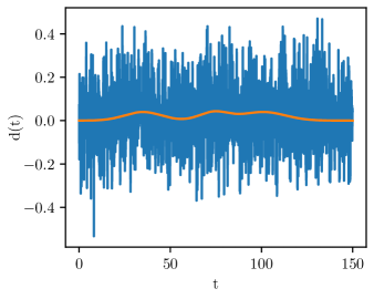
As a warm-up exercise, we consider a simple problem of fitting data with Gaussian pulses in the presence of Gaussian white noise.666The calculations in this subsection are performed in the accompanying jupyter notebook, pulse.ipynb, in the git repository linked above. Our data is a time series consisting of signal and noise :
| (5) |
Our signal model is a superposition of component functions given by
| (6) |
The mean , amplitude and the width are free to vary.
Our prior for the number of pulses is a discrete uniform distribution . The prior for the location of the first pulse is uniform over the domain of sampling times . The prior for the pulse is a uniform on the interval . This choice of prior ensures that the pulses are all ordered in time, but it is not a proximity prior enforcing any requirement for the closeness of neighboring pulses; we add that feature in the next subsection. For the amplitudes and widths, we employ a uniform priors in the range of [0.5,1.5] and [5,20] respectively. We create simulated data with a signal consisting of pulses plus Gaussian white noise with variance
| (7) |
The likelihood is
| (8) |
where is data, is signal template, is a discrete time, and is the noise. We show simulated data in Fig. 1 created with parameters summarized in Table 1.
| Pulse | Mean | Amplitude | Width |
|---|---|---|---|
| 1 | 35 | 1.0 | 10 |
| 2 | 74 | 0.8 | 8 |
| 3 | 101 | 1.2 | 12 |
We run tBilby using two different samplers: the nested sampler dynesty (Speagle, 2020) and the parallel-tempered Markov chain Monte Carlo sampler ptemcee (Vousden et al., 2015). For ptemcee, we update the number of pulses and the parameters for each pulse separately every time a new move is proposed in the sampling process. Since we are using ghost parameters, the sampler behaves as though it is exploring a fixed-dimensional space. In each iteration, we randomly add a pulse, remove a pulse, or keep fixed the number of pulses with equal probability. Since dynesty draws samples from priors, jumps in occur automatically by virtue of the discrete prior .
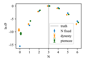
In Fig. 2, we plot the posterior odds
| (9) |
which compares the posterior support for different values of to the best-fit model.777Astute readers may notice that the right-hand side of Eq. 9 does not include the prior odds. This is because the prior odds in this case are unity.888We estimate the uncertainty in our calculations as follows: (10) Here, is the number of posterior samples for the hypothesis that the data are described by component functions while is the number of posterior samples describing the fiducial model—in this case, . The results obtained with dynesty are shown in orange while the results obtained with ptemcee are shown in green. As a sanity check, we also use dynesty to calculate the marginal likelihood for each value of with separate fixed-, which, combined with our prior of , we use to estimate the ground-truth posterior obtained without transdimensional inference. All three methods produce a similar distribution. Some values of are strongly disfavored, and so the transdimensional sample records no posterior samples for that value of . In such cases, we set an upper limit on . Both dynesty and ptemcee produce values that are consistent with the fixed- ground truth.
We compare the computational cost between the brute-force method of performing many fixed- runs and using tBilby. The fixed- runs for take roughly 4.6 times the sampling time of the tBilby dynesty run with the same sampler settings.999Note this is not a rigorous apples-to-apples comparison. For example, we do not require the same number of effective samples between the brute-force calculation and tBilby. However, it does provide a rough estimate of the improvement in computational cost for this particular problem. As expected, when we run different models separately, most computation time is spent exploring complicated models with large , which may not be the models with the highest Bayes factor. Since transdimensional sampling accounts for the Occam factor during sampling process, it automatically prevents the sampler exploring disfavoured regions of the parameter space.
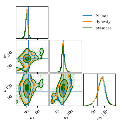
In Fig. 3, we present a corner plot showing the marginal posterior distribution of parameters given samples . As above, the fixed- ground truth is shown in blue while the results obtained with dynesty and ptemcee are shown in orange and green, respectively. All three posteriors produce consistent credible intervals.
3.2 GW150914
We now apply transdimensional inference to reconstruct the signal from the first gravitational-wave observation GW150914101010Strain data for GW150914 is accessed via Gravitational Wave Open Science Center (GWOSC) (LIGO Scientific Collaboration, Virgo Collaboration and KAGRA Collaboration, 2018). Following BayesWave (Cornish & Littenberg, 2015), we assume that the source of gravitational waves is elliptically polarized so that the cross-polarized strain is completely determined by the plus-polarized strain:111111For some bursting sources, it may be appropriate to adopt an unpolarized model so that is modelled independently from .
| (11) |
Here, is the ellipticity, which characterizes the polarization. We fit the binary black hole signal GW150914 using a superposition of sine-Gaussian wavelets; see Abbott (2016):
| (12) |
with . Here, is the amplitude, is the damping time, is the quality factor, is the central time, is the central frequency, and is the phase offset. The plus-polarized strain is the summation of several components
| (13) |
We adopt the following priors: the amplitudes follow log uniform priors between and we constrain the amplitude for the wavelet to be less than that of . The quality factor is taken from a uniform distribution on the interval , and follows a uniform distribution between 0 and with periodic boundary conditions.
For the wavelet, we adopt a uniform prior for and . For , we employ a proximity prior that require subsequent wavelets to be close to (but not too close to) the lower- wavelets. Following BayesWave (Cornish & Littenberg, 2015), we employ two-dimensional, hollowed-out Gaussians in the plane. For wavelet , the prior is
Here, is a normalisation constant. The width of the Gaussians is controlled by variables and . The variable controls the relative width of the hole in the middle of the Gaussian.121212Here, we adopt a slightly different convention than Cornish & Littenberg (2015). We employ a Gaussian of width hollowed out with a hole of width while Cornish & Littenberg (2015) uses a Gaussian of width hollowed out with a hole of width .. Following BayesWave (Cornish & Littenberg, 2015), we adopt . As for the width of the Gaussian, we set and . One can change the values of , , and to adapt the model to different problems. However, these three variables are not treated as free parameters from the perspective of the sampler.
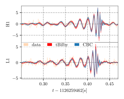
We analyze the LIGO–Virgo event GW150914 (Abbott et al., 2016a) using dynesty using the ghost parameter framework described above. We allow up to wavelets (25 total parameters). We combine samples from several runs weighted by the evidence of each run (Ashton & Khan, 2020). The sampling times range from to with 16 parallel processes running on a central processing unit. The reconstructed waveform is shown in Fig. 4 (red) alongside the whitened data (peach), and the compact binary coalescence (CBC) template fit shown as the blue curve.131313The CBC fit is obtained using the waveform approximant IMRPhenomXPHM (Pratten et al., 2021). The top panel is for the LIGO Hanford Observatory (LHO) while the bottom panel is for the LIGO Livingston Observatory (LLO). The wavelet fit produces a qualitatively similar reconstruction as the compact binary template fit. Both fits recover the morphology of key features in the whitened data. The wavelet fit produces a higher likelihood than the template fit (). Since we expect the template derived from general relativity to fit the signal, we interpret this as evidence that the wavelet fit is beginning to overfit features in the noise.
The posterior strongly favours over with probability allocated to . This motivates extending our prior range to . This follow-up test yields mixed results. On the one hand, some runs yield promising waveform reconstruction. On the other hand, the output is not stable run-to-run with current settings. This likely indicates that the sampler is failing to reliably converge for . In order to make further progress, it may be necessary to develop sampler settings that are better tuned for this transdimensional problem. We plan to adjust the implementation of dynesty in tBilby as a focus of future work.
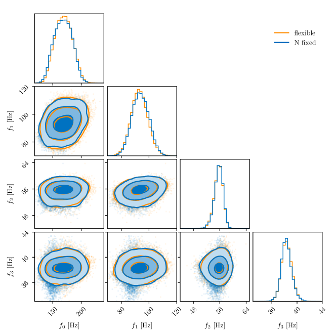
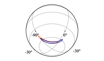
In Fig. 5, we show the posterior distributions for the frequencies of wavelets. The blue posterior distributions are obtained with a fixed analysis using Bilby, while the orange results are obtained allowing for any value of using tBilby. In Fig. 6 we show the sky localisation map for GW150914, where the blue curves are the 90% credible intervals obtained using the IMRPhenomXPHM waveform approximant and the orange curves are obtained using our transdimensional sine-Gaussian wavelet fit.
4 Discussion and conclusions
We introduce the tBilby package that facilitates transdimensional inference calculations with Bilby. Focusing, to start with, on time-domain models with a superposition of component functions, we provide examples where users can employ off-the-shelf samplers in Bilby to reconstruct signals with minimal alterations. The package includes example implementations of ghost parameters and proximity priors, a useful ingredient for this class of transdimensional problems. We show how tBilby can be used to perform a minimum-assumption fit of GW150914 with sine-Gaussian wavelets as in Abbott (2016).
For future work, we propose to improve the efficiency of tBilby through the use of more finely tuned samplers, designed for specific classes of problems of interest in gravitational-wave astronomy. Thanks to the modular design of Bilby, it is relatively easy to experiment with different options. While we find that dynesty produces well-converged fits to GW150914 for , we do not obtain reliable fits with ptemcee—at least using the default settings. And even our dynesty runs are currently limited to due to the scaling of the computational cost with . It may be necessary to employ custom jump proposals to improve convergence for ptemcee and/or to explore larger values of . Our work highlights the potential for carrying out transdimensional inference with nested sampling; see, e.g., Brewer et al. (2015).
We see this paper as the first step in a broader program to facilitate transdimensional inference with Bilby—in gravitational-wave astronomy and other contexts. We highlight a few priorities. First, as evidenced by work done with BayesLine (Littenberg & Cornish, 2015), transdimensional inference is a powerful tool for modelling the noise in gravitational-wave observatories; see also Gupta & Cornish (2023). Noise modelling naturally lends itself to transdimensional models because the noise power spectral density can be characterised by some fiducial shape plus a variable number of spectral features superposed on top. Transdimensional models can be used to obtain smooth fits of the noise power spectral density while characterizing instrumental lines and other features, enabling us to study the evolution of these features over the course of an observing run.
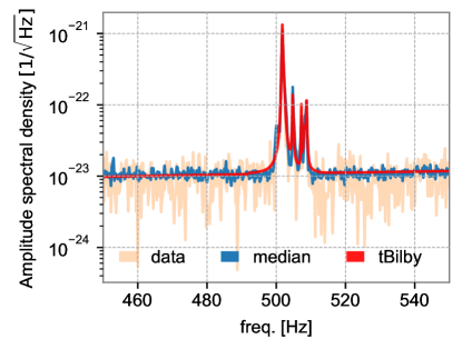
In Fig. 7, we show an example of a LIGO noise amplitude spectral density fit using tBilby. Inspired by Cahillane & Mansell (2022); Littenberg & Cornish (2015), our transdimensional model consists of a superposition of power laws (to model broadband noise) and Lorentzians (to model narrow lines). We analyze a segment of data immediately preceding the GW150914 event. For illustrative purposes, we focus on a narrow frequency band between . (Work is ongoing to develop a model that reliably fits the entire LIGO observing band.) The transdimensional model (red) succeeds in fitting the data (peach) including several narrowband features. The posterior for and for this model peak at and , respectively, even though the priors for these parameters extend up to 5 and 12, respectively. A comprehensive study will be detailed in a forthcoming publication. Code to reproduce this plot is available in the accompanying asd.ipynb notebook.
In terms of non-stationary noise modelling, we are also excited about the application of transdimensional sampling to model potential glitches simultaneously with compact binary signals (Chatziioannou et al., 2021a; Hourihane et al., 2022). This work may help astronomers to better interpret gravitational-wave events with potential data quality problems (Payne et al., 2022).
Second, we envision extending tBilby to build more flexible models describing the population properties of binary black holes and neutron stars; see, e.g., Toubiana et al. (2023). For example, one may wish to model the distribution of primary black hole mass mass distribution with a variable number of peaks and troughs. Recent studies have highlighted the usefulness of flexible models to identify structure that might be missing from astrophysically inspired phenomenological models; see, e.g., Tiwari & Fairhurst (2021); Edelman et al. (2022, 2023).
Finally, we propose to develop tBilby for applications beyond terrestrial gravitational-wave observatories. For example, pulsar timing measurements, which can be used to measure nanohertz gravitational-waves (Agazie et al., 2023; Antoniadis et al., 2023; Reardon et al., 2023; Xu et al., 2023), rely on measurements of the time of arrival of arbitrarily shaped radio pulses. By modelling these pulses using a superposition of component functions, it is sometimes possible to identify and account for aberrant behaviour in the pulsar evolution, ultimately improving sensitivity for gravitational-wave searches (Nathan et al., 2023). Transdimensional models may prove useful determining the number of component functions used in these fits. Of course, this is just one example. It is our hope that the tBilby package will facilitate the development of numerous transdimensional models for physics and astronomy.
Appendix A Code design
The objective of tBilby is to provide a comprehensive toolkit for handling transdimensional sampling. The tBilby package offers flexibility and automation. As outlined in this Paper, the development of tBilby is part of a long-term project with multiple goals. At present, we have constrained the package to a set of essential tools and examples. tBilby’s design philosophy closely aligns with that of Bilby, emphasizing open-source code, modularity, generality, and usability (Ashton et al., 2019). Based on the ideas and infrastructure of Bilby, tBilby ensures a relatively smooth user experience, particularly for experienced users. Furthermore, we reinforce this philosophy by mandating that the sole requirement for tBilby is an installation of Bilby.
The structure of tBilby closely mirrors that of Bilby, with the core module including base, prior, and sampler modules, alongside an additional folder dedicated to examples. The base module contains fundamental functionality for constructing transdimensional models and defining transdimensional priors. The prior folder houses priors intended for transdimensional sampling, while the sampler module facilitates support for transdimensional samplers.
The key building block of a transdimensional model in tBilby is the transdimensional parameter, which refers to a parameter of a component function that has multiple “orders” (in this language, each sine-Gaussian is a different order). Another fundamental concept is the transdimensional prior, which constitutes a set of priors related to a transdimensional parameter and which is attached to the parameter’s order. Transdimensional models with proximity priors employ conditional statements. These two elements serve as the basic building blocks.
For practical purposes, transdimensional priors in tBilby are categorized into four types: (i) transdimensional nested conditional priors, (ii) transdimensional conditional priors, (iii) conditional priors, and (iv) unconditional priors.141414Examples employing each of the prior types can be found at the git repository. Transdimensional nested conditional priors are defined by their dependence on previously sampled parameters of the same component function. If we assume that the current order being sampled is , these priors depend on parameters of orders etc.
Transdimensional conditional priors, on the other hand, are dependent on parameters from all sampled orders of a component function, denoted by etc. Conditional priors rely on a set of non-transdimensional parameters, whereas unconditional priors are independent of other parameters. The most general prior may combine elements of all these types, except for the last type, which by definition is an independent prior. In this framework, the most general form of a prior for transdimensional parameter is:
The variable represents another set of transdimensional parameters of the same order as the component function so that does not depend on . Meanwhile, signifies another set of transdimensional parameters that depend on all available orders of the component function. Finally, are parameters that may or may not be part of the component function parameters.
By allowing for the definition of conditional transdimensional priors, users can uniquely specify priors for each transdimensional parameter. Practically, this involves defining a class that inherits from a predefined transdimensional prior class and implementing an abstract function to define the mathematical relation between the conditional parameters and prior properties (this is a generalization of Bilby’s condition function, which is required when defining a conditional prior).
Facilitating such versatility and control over the priors allows users to gain flexibility in manipulating the prior distribution to suit their specific needs. The flexibility of tBilby’s extends further, enabling the construction of function superposition, each potentially comprising a different number of component functions. For instance, the LIGO noise power spectral density may be represented as a combination of several power law functions along with multiple Cauchy-like functions, addressing distinct spectral characteristics (Littenberg & Cornish, 2015). Furthermore, tBilby offers supplementary tools for removing ghost parameters and generating relevant corner plots, thereby simplifying the analysis of component functions and individual transdimensional parameters.
Appendix B Ghost parameter
The method outlined here is similar to Liu et al. (2023) who performed transdimensional inference using Bilby for gravitational-wave lensing study. In the ghost parameter framework, we introduce extra parameters that do not actually change the likelihood, and therefore do not change the posteriors for the original parameters—as long as the ghost-parameter prior is correctly normalized. For example, we consider the situation in Section 3.1 when . The signal is only determined by while represents the ghost parameters. In this case, the posterior is
| (B1) |
The conditional posterior given can be written as
| (B2) |
As the priors for the extra parameters are properly normalized by definition, i.e.,
| (B3) |
the marginalized posterior for is equivalent to the case where there are no extra parameters:
| (B4) | ||||
Now we take a look at the denominator of Eq. B2. It is actually the marginal likelihood of in transdimensional sampling:
| (B5) |
Meanwhile, we note it is essentially a normalization factor, so the expression can be also written as
| (B6) | ||||
We make use of the fact that the priors for ghost parameters are properly normalized again.
So the model selection result of our transdimesional problem with ghost parameters is valid regardless of the inclusion of ghost parameters as the likelihood is correctly defined as the case without the implementation of ghost parameters.
As a comparison, the detailed balance equations of traditional reversible jump Markov chain Monte Carlo without ghost parameters is written as
| (B7) |
where is the target distribution, i.e., posteriors in Bayesian inference, is the proposal for samples in Markov chain Monte Carlo sampling and is the acceptance probability. This makes use of the trade-off between higher dimension proposals in the left-hand side and higher dimension posteriors in the right-hand side.
With the implementation of ghost parameters, we artificially add extra dimensions for posteriors and proposals in both side with the detailed balance equation written as
| (B8) |
As we show above, in the case where are not used in the evaluation of the likelihood, the posteriors could be written as two independent parts
| (B9) |
Thus, if we choose a proper reversible proposal distribution to make
then the detailed balance can be written as
| (B10) | ||||
This reduces to Eq.B7 where we do not implement ghost parameters. In fact, it is not necessary to set up special proposals for ghost parameters. With arbitrary proposal distributions, the sampling result with the implementation of ghost parameters will always be consistent with the situation without ghost parameters as the statistical average of acceptance rate over the entire parameters space.
References
- Aasi et al. (2015) Aasi, J., et al. 2015, Class. Quant. Grav., 32, 074001
- Abbott (2016) Abbott, B. P. 2016, Phys. Rev. D, 93, 122004
- Abbott et al. (2016a) Abbott, B. P., et al. 2016a, Phys. Rev. Lett., 116, 061102
- Abbott et al. (2016b) —. 2016b, Phys. Rev. Lett., 116, 241102
- Abbott et al. (2016c) —. 2016c, Phys. Rev. Lett., 116, 221101
- Abbott et al. (2017) —. 2017, Nature, 551, 85
- Abbott et al. (2018) —. 2018, Phys. Rev. Lett., 121, 161101
- Abbott et al. (2021) Abbott, R., et al. 2021, Astrophys. J. Lett., 913, L7
- Abbott et al. (2023) —. 2023, Phys. Rev. X, 13, 011048
- Acernese et al. (2015) Acernese, F., et al. 2015, Class. Quant. Grav., 32, 024001
- Agazie et al. (2023) Agazie, G., et al. 2023, Astrophys. J. Lett., 956, L3
- Antoniadis et al. (2023) Antoniadis, J., et al. 2023, Astron. Astrophys., 678, A50
- Ashton & Dietrich (2022) Ashton, G., & Dietrich, T. 2022, Nature Astronomy, 6, 961
- Ashton & Khan (2020) Ashton, G., & Khan, S. 2020, Physical Review D, 101, 064037
- Ashton et al. (2019) Ashton, G., et al. 2019, Astrophys. J. Supp., 241, 27
- Aso et al. (2013) Aso, Y., Michimura, Y., Somiya, K., et al. 2013, Phys. Rev. D, 88, 043007
- Brewer et al. (2015) Brewer, B. J., Huijser, D., & Lewis, G. F. 2015, Mon. Not. R. Ast. Soc., 455, 1819
- Cahillane & Mansell (2022) Cahillane, C., & Mansell, G. 2022, Galaxies, 10, 36, doi: 10.3390/galaxies10010036
- Chatziioannou et al. (2021a) Chatziioannou, K., Cornish, N., Wijngaarden, M., & Littenberg, T. B. 2021a, Physical Review D, 103, 044013
- Chatziioannou et al. (2021b) Chatziioannou, K., Isi, M., Haster, C.-J., & Littenberg, T. B. 2021b, Phys. Rev. D, 104, 044005
- Cornish & Littenberg (2015) Cornish, N. J., & Littenberg, T. B. 2015, Class. Quantum Grav., 32, 135012
- Cornish et al. (2021) Cornish, N. J., Littenberg, T. B., Bècsy, B., et al. 2021, Phys. Rev. D, 103, 044006
- Dàlya et al. (2021) Dàlya, G., Raffai, P., & Bècsy, B. 2021, Bayesian reconstruction of gravitational-wave signals from binary black holes with nonzero eccentricities
- Davis et al. (2022) Davis, D., Littenberg, T. B., Romero-Shaw, I. M., et al. 2022, Class. Quantum Grav., 39, 245013
- Edelman et al. (2022) Edelman, B., Doctor, Z., Godfrey, J., & Farr, B. 2022, Astrophys. J., 924, 101
- Edelman et al. (2023) Edelman, B., Farr, B., & Doctor, Z. 2023, Astrophys. J., 946, 16
- Ellis & Cornish (2016) Ellis, J., & Cornish, N. 2016, Phys. Rev. D, 93, 084048
- Green (1995) Green, P. J. 1995, Biometrika, 82, 711
- Gupta & Cornish (2023) Gupta, T., & Cornish, N. 2023, Phys. Rev. D, 109, 064040
- Hotokezaka et al. (2019) Hotokezaka, K., Nakar, E., Gottlieb, O., et al. 2019, Nature, 3, 940
- Hourihane et al. (2022) Hourihane, S., Chatziioannou, K., Wijngaarden, M., et al. 2022, Physical Review D, 106, 042006
- Johnson-McDaniel et al. (2022) Johnson-McDaniel, N. K., Ghosh, A., Ghonge, S., et al. 2022, Phys. Rev. D, 105, 044020
- Karnesis et al. (2023) Karnesis, N., Katz, M. L., Korsakova, N., Gair, J. R., & Stergioulas, N. 2023, Eryn: A multi-purpose sampler for Bayesian inference
- Klimenko et al. (2008) Klimenko, S., Yakushin, I., Mercer, A., & Mitselmakher, G. 2008, Class. Quantum Grav., 25, 114029
- Kronland-Martinet et al. (1987) Kronland-Martinet, R., Morlet, J., & Grossmann, A. 1987, International Journal of Pattern Recognition and Artificial Intelligence, 1, 273
- LIGO Scientific Collaboration, Virgo Collaboration and KAGRA Collaboration (2018) LIGO Scientific Collaboration, Virgo Collaboration and KAGRA Collaboration. 2018, GWTC-1 Data Release, https://gwosc.org/GWTC-1/
- Littenberg et al. (2020) Littenberg, T., Cornish, N., Lackeos, K., & Robson, T. 2020, Phys. Rev. D, 101, 123021
- Littenberg & Cornish (2010) Littenberg, T. B., & Cornish, N. J. 2010, Phys. Rev. D, 82, 103007
- Littenberg & Cornish (2015) —. 2015, Phys. Rev. D, 91, 084034
- Littenberg et al. (2016) Littenberg, T. B., Kanner, J. B., Cornish, N. J., & Millhouse, M. 2016, Phys. Rev. D, 94, 044050
- Liu et al. (2023) Liu, A., Wong, I. C. F., Leong, S. H. W., et al. 2023, Monthly Notices of the Royal Astronomical Society, 525, 4149
- Millhouse et al. (2018) Millhouse, M., Cornish, N. J., & Littenberg, T. 2018, Phys. Rev. D, 97, 104057
- Miravet-Tenés et al. (2023) Miravet-Tenés, M., Florencia L. Castillo, R. D. P., Cerdá-Durán, P., & Font, J. A. 2023, Phys. Rev. D, 107, 103053
- Nathan et al. (2023) Nathan, R. S., et al. 2023, Mon. Not. R. Ast. Soc., 523, 4405
- Pankow et al. (2018) Pankow, C., et al. 2018, Phys. Rev. D, 98, 084016
- Pannarale et al. (2021) Pannarale, F., Macas1, R., & Sutton, P. J. 2021, Class. Quantum Grav., 36, 035011
- Payne et al. (2022) Payne, E., Hourihane, S., Golomb, J., et al. 2022, Phys. Rev. D, 106, 104017
- Pratten et al. (2021) Pratten, G., et al. 2021, Phys. Rev. D, 103, 104056
- Raza et al. (2022) Raza, N., McIver, J., Dàlya, G., & Raffai, P. 2022, Phys. Rev. D, 106, 063014
- Reardon et al. (2023) Reardon, D. J., et al. 2023, Astrophys. J. Lett., 951, L6
- Romero-Shaw et al. (2020) Romero-Shaw, I. M., et al. 2020, Mon. Not. R. Ast. Soc., 499, 3295
- Speagle (2020) Speagle, J. S. 2020, Mon. Not. R. Ast. Soc., 493, 3132
- Tiwari & Fairhurst (2021) Tiwari, V., & Fairhurst, S. 2021, Astrophys. J. Lett., 913, L19
- Toubiana et al. (2023) Toubiana, A., Katz, M. L., & Gair, J. R. 2023, Mon. Not. R. Ast. Soc., 524, 5844
- Vousden et al. (2015) Vousden, W. D., Farr, W. M., & Mandel, I. 2015, mnras, 455, 1919
- Xu et al. (2023) Xu, H., et al. 2023, Res. Astrono. Astrophys., 23, 075024
- Yi Shuen C. Lee & Melatos (2021) Yi Shuen C. Lee, M. M., & Melatos, A. 2021, Phys. Rev. D, 103, 062002