Spatial estimation of virus infection propensity in hosts determined from GPS-based space-time locations

Abstract

Identifying areas in a landscape where individuals have a higher probability of becoming infected with a pathogen is a crucial step towards disease management. Our study data consists of GPS-based tracks of individual white-tailed deer (Odocoileus virginianus) and three exotic Cervid species moving freely in a 172-ha high-fenced game preserve over given time periods. A serological test was performed on each individual to measure the antibody concentration of epizootic hemorrhagic disease virus (EHDV) for each of three serotypes (EHDV-1, -2, and -6) at the beginning and at the end of each tracking period. EHDV is a vector-borne viral disease indirectly transmitted between ruminant hosts by biting midges (Culicoides spp.). The purpose of this study is to estimate the spatial distribution of infection propensity by performing an epidemiological tomography of a region using tracers. We model the data as a binomial linear inverse problem, where spatial coherence is enforced with a total variation regularization. The smoothness of the reconstructed propensity map is selected by the quantile universal threshold, which can also test the null hypothesis that the propensity map is spatially constant. We apply our method to simulated and real data, showing good statistical properties during simulations and consistent results and interpretations compared to intensive field estimations.

1 Introduction

Predicting spatial disease risk, specifically identifying areas in which individuals have higher probability of becoming infected is a crucial step towards management of human, livestock, and wildlife diseases (Morris and Blackburn, 2016). Although spatial prediction of infectious diseases has traditionally been understudied (Ostfeld et al., 2005; Kirby et al., 2017), rapid growth of new algorithms and technology has improved spatial inferences of disease dynamics (Ostfeld et al., 2005; Riley et al., 2015; Kirby et al., 2017). In spatial epidemiology, many studies are focused on diseases with direct transmission (i.e., in which direct contact between a susceptible and infected individual leads to transmission of the pathogen) but many important human epidemics (e.g., tropical vector borne diseases, Cholera, Salmonella) and domestic and wildlife zoonoses (e.g., brucellosis, anthrax, macroparasites) have indirect transmission (Hollingsworth et al., 2015).

Indirectly transmitted diseases are those where direct contact between a susceptible and an infected individual does not lead to infection. Instead, disease transmission is mediated by a vector transmitting the pathogen from an infected to naive host through a bite (e.g., malaria parasites through mosquito bites). Malaria, dengue virus, and Lyme’s disease, are three of the most common vector borne diseases for which there is substantial spatially implicit and explicit research on their dynamics (Torres-Sorando and Rodriguez, 1997; Killilea et al., 2008; Messina et al., 2015). Alternatively, a pathogen may not require a vector to infect new individuals but instead the pathogens have environmental reservoirs from which hosts are infected. Anthrax, cholera, salmonellosis, or similar bacterial gastric infections are examples of non-vector borne indirectly transmitted diseases (Ostfeld et al., 2005). Although it is of extreme importance to understand in detail their dynamics through traditional compartmental models (Keeling et al., 2008), most of these models are spatially implicit and during epidemics, spatial prediction of risk may allow for better predictions on the environmental drivers of disease risk and identify areas that require immediate control and isolation (Ostfeld et al., 2005).

Inferences about the risk of indirectly transmitted diseases rely on the spatial distribution of cases or some knowledge about their ecology and disease dynamics. For example, spatially explicit compartmental models require either previous knowledge about transmission rates or transition rates from one compartment to another or data driven estimation of these parameters. In either case, it requires an a priori hypothesis about how the disease spreads in the population. Other types of models rely on the overlap between vectors and hosts to understand and predict areas with high disease risk. In a changing world however, there are many new types of directly and indirectly transmitted diseases for which there is no knowledge about their ecology, behavior or dynamics (Harvell et al., 2002; Patz et al., 2008). Nonetheless, spatially predicting the areas in which individuals have higher risk of becoming sick without any knowledge of the speed or intensity of transmission can be a powerful tool for rapid control and mitigation to decrease the likelihood of a disease outbreak becoming an epidemic. Such task may be achieved by simply studying the spatial distribution of diseases by focusing on the movement of infected and naive individuals.

In this study, we take a novel approach to predict the areas in which organisms have a higher risk of becoming infected from an indirectly transmitted disease. To test our approach we use movement data from white-tailed (WTD), Pere David (ED), Fallow (DD) and Elk deer (CC) in a 172-ha high-fenced ranch in Florida, USA. In the ranch there is a high prevalence of several serotypes of Epizootic Hemorrhagic Disease Virus (EHDV) which causes severe clinical signs such as hemorrhaging, edema, hoof-sloughing, oral lesions and death, principally in WTD but it affects other Cervid species as well such as ED, DD and CC. EHDV is transmitted by biting midges from the genus Culicoides and in southeastern United States, Culicoides stellifer and Culicoides venustus have been identified as the competent EHDV vectors. There has been substantial research on this high-fenced ranch regarding the abundance, host preference, spatial distribution (McGregor et al., 2019b; Dinh et al., 2021a), and vector competence (McGregor et al., 2019a) of biting midges. Additionally, work has described seasonal and inter-annual home ranges (Orange et al., 2021b), home range visitation and fidelity (Dinh et al., 2020) and resource selection (Dinh et al., 2021b) of WTD on the ranch. The prevalence of EHDV in WTD and other exotic species has also been described (Cauvin et al., 2020; Orange et al., 2021a), but to date, disease risk on the ranch has been estimated by inferring resource selection in deer and overlap with areas of high biting midge abundance.

1.1 Data description

Table 1: Animals tracked to estimate the disease risk of three EHDV serotypes in White-tailed deer and three exotic Cervid species. We show Animal ID, sex, tracking year, start and end date of tracking period, total number of days each animal was tracked and whether the animal was seronegative (0) or seropositive (1) for each serotype at the end of the tracking period. NA values indicate animals for which serostatus was unavailable. All animals were seronegative at the beginning of the tracking period. NA values indicate animals for which serostatus was unavailable. OV = Odocoileus virginianus, White-tailed deer. DD = Dama dama, Fallow deer. ED = Elaphurus davidianus, Pere David deer. CC = Cervus canadensis, Elk deer.

Accession ID	Sex	Year	Date Collared	Date End	Days	EHDV-1	EHDV-2	EHDV-6
2015_OV10	M	2015	5/27/15	11/3/15	160	1	1	0
2015_OV11	F	2015	5/29/15	10/13/15	137	0	NA	0
2015_OV12	M	2015	5/27/15	9/23/15	119	1	1	0
2015_OV6	M	2015	5/28/15	10/3/15	128	1	NA	0
2015_OV7	M	2015	5/29/15	10/13/15	137	1	1	0
2015_OV8	M	2015	5/28/15	10/13/15	137	1	NA	0
2015_OV9	M	2015	5/27/15	10/3/15	129	1	0	0
OV059	F	2016	4/13/16	9/21/16	161	1	1	1
OV062	M	2016	4/13/16	9/21/16	161	NA	1	1
OV063	F	2015	5/28/15	10/15/15	140	1	NA	0
OV063	F	2016	4/13/16	10/3/16	173	1	1	1
OV064	F	2016	4/14/16	9/17/16	156	1	1	1
OV065	M	2015	5/29/15	10/12/15	136	1	1	0
OV065	M	2016	4/14/16	9/21/16	160	1	1	1
OV067	M	2016	4/14/16	9/2/16	141	NA	NA	1
OV069	F	2016	4/14/16	10/4/16	173	1	1	NA
OV070	F	2016	4/14/16	9/22/16	161	1	1	1
OV071	M	2015	5/27/15	10/13/15	139	1	NA	1
OV071	M	2016	4/14/16	9/22/16	160	1	1	1
OV072	M	2016	4/14/16	9/21/16	160	NA	NA	0
OV073	M	2016	4/15/16	9/23/16	161	1	NA	1
OV074	M	2015	5/28/15	10/14/15	139	1	1	0
OV074	M	2016	4/15/16	9/21/16	159	1	1	1
DD001	F	2016	4/15/16	4/3/17	353	0	1	0
DD2015_1	M	2015	5/28/15	10/12/15	137	1	1	0
DD2015_2	M	2015	5/29/15	10/14/15	138	0	0	0
ED001	F	2016	4/15/16	9/21/16	159	1	1	0
ED2015_1	M	2015	5/29/15	10/12/15	136	0	1	0
CC2015_1	M	2015	5/27/15	9/2/15	98	1	1	1
CC2015_2	M	2015	5/29/15	10/12/15	136	0	1	0

Data consist of movement of WTD, DD, ED and CC in a 172-ha high-fenced ranch in Florida dedicated to big-game hunting, in which 130-150 WTD and a similar number of non-native Cervids and bovids were maintained at the time of the study. For this study we excluded animals from different families other than Cervidae because of their differences in behavior and propensity in getting infected with EHDV. There were 12 stationary supplemental feeders located across the preserve which were filled twice a week so that food is consistently available. In total, we tracked the movement of 26 animals (8 females, 18 males) during the EHDV risk period, then estimated as  May - October ((Dinh et al., 2020), in each 2015 and 2016. Specifically, WTD were captured and GPS collared in spring (April/May), ahead of the EHDV transmission season and recaptured in fall (September/October), so that collars could be removed. From the 26 individuals, four were tracked during both 2015 and 2016 and were used for the analysis after serological testing. Consequently our data set consisted of 30 tracks from 26 individuals that were tracked for 149 days on average. Individuals were captured and radio tagged with GPS collars and programmed to collect a GPS location every 15 minutes for some deer and and up to 120 minutes for others (collar battery size was dictated by animal size; smaller collar batteries were set to record fewer points). Capture procedures are described in detail elsewhere (Cauvin et al., 2020; Dinh et al., 2020). Briefly, animals were immobilized with cartridge or air powered darts, monitored, collared, bled, and released. A blood sample was obtained from each captured individual at the time of initial capture and again later in the year when GPS collars were recovered. Each blood sample was tested for the presence of EHDV-1, EHDV-2 and EHDV-6 antibody titers using a virus neutralization test (Stallknecht et al., 1996) performed at Texas A&M University. The testing procedure is described in detail elsewhere (Cauvin et al., 2020). For this study, we defined animals as positive or negative for each virus type using previous cutoffs (Cauvin et al., 2020). All individuals were recaptured after a fixed period (see Table 1). A first group of WTD were captured and collared in the spring of 2015 and then these animals were recaptured and collars were removed in the Fall of 2015. Then a second group of animals were captured and collared in the Spring of 2016 and then these animals were recaptured and collars were removed in the fall of 2016. Four of these animals were captured and collared in both years while others were captured in only one year. We treated the four individuals captured during both time periods as independent tracks for analyses. Deer capture and handling protocols were developed by JKB and the ranch wildlife manager and approved by the Institutional Animal Care and Use Committee at the University of Florida (UF IACUC Protocols #201508838 and #201609412).

To set notation for the collected data of sample size $n$, each individual has a blood test at time $0$ leading to concentrations of four different antibodies $c_{i,m}(0)$, and at time $t_{i}$ leading to concentrations $c_{i,m}(t_{i})$, $m=1,\ldots,3$ (EHDV-1, EHDV-2 and EHDV-6 antibodies). From these concentrations, one can declare whether the $i$th individual got infected by virus $m$ during the time period, leading to binary responses $y_{i,m}=1_{\{c_{i,m}(t_{i})>c_{i,m}(0)\}}$ for $i=1,\ldots,n$ and $m=1,\ldots,3$. Let ${\bf y}_{i}=(y_{i,1},\ldots,y_{i,3})$ be the vector of binary indicators of contamination of individual $i$ by any of the three EHDV viruses, for $i=1,\ldots,n$. Individuals move differently in the fenced area $\Omega$, as observed by the GPS tracking system. To map the spatial variability in infection propensity $\mu$, the fenced area $\Omega$ is spatially descretized and partitioned over equal small units $\omega^{j,k}$ indexed by latitude $j$ and longitude $k$, for $(j,k)\in{\cal F}$. The level of discretization $p=|{\cal F}|$ is chosen by the practitioner: the larger $p$, the finer the spatial discretization, but the more parameters to estimate. Correspondingly, each area $\omega^{j,k}$ has the propensity $\mu(\omega^{j,k})$ of contaminating a species with a disease during a unit time period, where $\mu$ is a function of localization $\omega^{j,k}$ in $\Omega$. Using the GPS recordings, one can, for each individual $i$, calculate the total time $x^{j,k}_{i}$ spent in each small area $\omega^{j,k}$ between its starting time until time $t_{i}$; so let ${\bf x}_{i}=\{x_{i}^{j,k}\}_{(j,k)\in{\cal F}}$ be the vector of total time spent in location $\omega^{j,k}$ for individual $i$, for $i=1,\ldots,n$. The goal is to estimate the propensity maps ${\boldsymbol{\mu}}_{m}=\{\mu_{m}(\omega^{j,k})\}_{(j,k)\in{\cal F}}$ ($m=1,\ldots,3$, one map per EHDV virus) based on the information contained in the data $({\bf y}_{i},{\bf x}_{i})_{i=1,\ldots,n}$.

1.2 Spatial mapping of diseases from GPS tracking

The first step into the management of these indirectly transmitted diseases is to understand the spatial distribution and the areas in which individuals have a higher risk of becoming infected (Morris and Blackburn, 2016) and how animals use those spaces, and show home range and seasonal range fidelity ((Dinh et al., 2020; Orange et al., 2021b). It is thus useful to describe with basic spatial statistics the distribution and the spatial autocorrelation of geographic locations of animals across time (de Thoisy et al., 2020; Albery et al., 2022; Dougherty et al., 2018). Further exploration of the spatial distribution of the known cases includes exploring the climatic envelope or the abiotic niche (that is, the suit of environmental conditions that favor new infections) of vectors or pathogens (Ostfeld et al., 2005; de Thoisy et al., 2020). Two commonly used methods are Maxent and GARP (Ahmed et al., 2015) for which presence of the disease is climatically characterized using a set of environmental variables that are thought to physiologically constrain the distribution of the species (Estrada-Pena et al., 2014). In Maxent, the final distribution of species is predicted by determining the conditional probability that a species is present given environmental variables throughout the landscape (Elith et al., 2011). Alternatively, GARP uses an iterative modelling approach to generate a series of rulesets that predict the presence of the pathogen in the landscape given the environmental conditions. Through iterations of a genetic algorithm, the rules are changed through mutations, insertions, deletions, etc., to find the best set of rules that accurately predicts presence points (Stockwell, 1999). Other methods have been proposed based on different assumptions and modelling strategies (Ahmed et al., 2015).

One disadvantage of predicting disease risk based on the presence of cases is that usually these presence points are based on identification of infected individuals (Ostfeld et al., 2005). In most cases, and in most diseases, individuals move substantially through the landscape before being diagnosed. Thus, using information about individual diagnosis coupled with animal movements can allow researchers to better identify areas in which individuals are disproportionately being infected (Ostfeld et al., 2005). These host movements are seldom accounted for in disease niche modeling or spatial prediction of disease risk. Yet, the use of an animal’s home range and habitat selection has proved to be useful in identifying transmission risk of some wildlife zoonoses (Ragg and Moller, 2000) caused by environmentally-mediated pathogens, like Mycobacterium bovis or Bacillus anthracis, the causes of bovine tuberculosis and anthrax, respectively ((Ragg and Moller, 2000; Dougherty et al., 2022). Coupling environmental information with host disease movement can improve prediction from the potential distribution of the pathogen to the realized distribution of the disease.

More recently, there has been an increased use of movement data from infected individuals to infer areas with higher infection risk (Dougherty et al., 2018). Most of these applications are based on human infections such as HIV and H1N1 outbreaks (Brdar et al., 2016; Frias-Martinez et al., 2012). In such cases, disease risk is inferred based on the spatial prediction of disease prevalence and related to the movement of the organisms to produce an hypothesis about the factor influencing high prevalence. Some of these approaches include spatially explicit compartmental models for the dissemination of infectious diseases (Lima et al., 2015), but they do not directly tackle the problem of predicting disease risk without underlying assumptions about the disease dynamics.

2 Total variation regularization of GLM

2.1 Model

Since the three EHDV serotype antibodies considered have their own specificities, we consider three separate models, so we call the disease marker $y_{i}$ (instead of $y_{i,1}$ for EHDV-1, $y_{i,2}$ for EHDV-2 and $y_{i,3}$ for EHDV-6) for $i=1,\ldots,n$ regardless whether we are considering EHDV-1, -2 or -6. The common approach sees $y_{i}$ as a realization of the random variable $Y_{i}\sim\operatorname{Bernoulli}(\epsilon_{i})$, where the probability $\epsilon_{i}$ of being infected depends on where the $i$th individual spent its time in the fenced area. In particular $\epsilon_{i}$ should be high if the $i$th individual spent long periods of time in areas of high infection propensity; in other words, $\epsilon_{i}$ should be high when high total times $x_{i}^{j,k}$ are observed in regions $\omega^{j,k}$ where the unknown propensity $\mu(\omega^{j,k})$ is high. A simple, yet useful and realistic, model is the generalized linear model (Nelder and Wedderburn, 1972) which assumes $g(\epsilon_{i})={\bf x}_{i}^{\rm T}{\boldsymbol{\mu}}$, where the logit link function $g(\epsilon)=\log(\epsilon/(1-\epsilon))$ maps $(0,1)$ into ${\mathbb{R}}$. Letting ${\bf Y}=(Y_{1},\ldots,Y_{n})$ and $X$ be the $n\times p$ matrix which $i$th row is ${\bf x}_{i}^{\rm T}$, the model is

$${\bf Y}\sim\operatorname{Bernoulli}(g^{-1}(X{\boldsymbol{\mu}})),$$ (1)

where ${\boldsymbol{\mu}}$ is the unknown propensity vector. So the model can be seen as a tomographic linear inverse problem, for which the individuals are probing the space with their distinct movements reflected in the data matrix $X$ of total times visting the lattice system in $\Omega$. Instead of directly measuring the sources of where the virus is spreading, the information is indirectly measured on individuals living in potentially infecting areas.

2.2 Estimation

The vector of infection propensity ${\boldsymbol{\mu}}$ has length $p=|{\cal F}|$, the cardinality of the lattice system that segments the fenced area $\Omega$. In our application the number of individuals is small, so we choose a fairly coarse segmentation of the fenced area into $p=200$ cells. Regularization is needed, and owing to the spatial structure of the problem, we impose a smoothness constraint on ${\boldsymbol{\mu}}$. An entry $\mu_{l}$ of the vector of infection propensity ${\boldsymbol{\mu}}$ corresponds to a small region $\omega^{j,k}$ in $\Omega$. Each region $(j,k)$ is associated to an entry of ${\boldsymbol{\mu}}$, call it $l$. Each region $(j,k)$ (associated to $l$) has neighbors: call $\partial l$ the set of entries of ${\boldsymbol{\mu}}$ corresponding to the neighbors of $(j,k)$. Because of the spatial structure of ${\boldsymbol{\mu}}$ which maps the propensity of catching a virus somewhere in the ranch, one believes that the value of $\mu_{l}$ is close to $\mu_{l^{\prime}}$ for $l^{\prime}\in\partial l$; here we consider the north-south-east-west neighborhood of a cell. Total variation (TV) regularization (Rudin et al., 1992) allows to impose this type of smoothness belief by solving

$$\min_{{\boldsymbol{\mu}}\in{\mathbb{R}}^{p}}-\log{\rm L}(g^{-1}(X{\boldsymbol{\mu}});{\bf y})+\lambda\sum_{l=1}^{p}\sum_{l^{\prime}\in\partial l}|\mu_{l}-\mu_{l^{\prime}}|,$$ (2)

where $L$ is the likelihood associated to (1), ${\bf y}$ is the vector of infection indicator per individual, $X$ is total time matrix per individual (lines) spent in area $\omega^{j,k}$ (column), and ${\boldsymbol{\mu}}$ is the two-dimensional surface to reconstruct. The regularization parameter $\lambda>0$ controls the smoothness of the estimate $\hat{\boldsymbol{\mu}}_{\lambda}$ solution to (2). One standard selection of $\lambda$ is cross-validation, which requires $n$ large for a stable estimation. In our situation, the number $n$ of individuals is rather small, so we employ the quantile universal threshold (Giacobino et al., 2017) that is geared towards estimating and testing the propensity map ${\boldsymbol{\mu}}$. The quantile universal threshold is based on calibrating a choice of $\lambda$ under the null hypothesis $H_{0}$ that the propensity map is constant (that is, no regions more infectious than others): its goal is to retrieve a constant map with high probability under $H_{0}$. This choice of $\lambda$ remains performant under alternative hypotheses as supported by the LASSO theory (Tibshirani, 1996; Bühlmann and van de Geer, 2011) and total variation (Rudin et al., 1992; Sardy and Monajemi, 2019). Deriving the quantile universal threshold for our TV-estimator (2) is based on the following property.

Property 1

Assuming the entries of the response data ${\bf y}$ are not all identical (all ones or all zeros), there exists a finite $\lambda>0$ for which the solution $\hat{\boldsymbol{\mu}}_{\lambda}$ to (2) is a constant propensity map across $\Omega$. Moreover the smallest such $\lambda$ is given by the zero-thresholding function

$$\lambda_{0}({\bf y},X)=\min_{{\boldsymbol{\omega}}\in{\mathbb{R}}^{q}}\|{\boldsymbol{\omega}}\|_{\infty}\quad{\rm s.t.}\quad X^{\rm T}({\boldsymbol{\epsilon}}-{\bf y})+D^{\rm T}{\boldsymbol{\omega}}={\bf 0},\ {\boldsymbol{\epsilon}}=g^{-1}(\hat{\beta}_{0}X{\bf 1}),\ \hat{\beta}_{0}=\operatorname*{\arg\!\min}_{\beta_{0}\in{\mathbb{R}}}h(\beta_{0}{\bf 1};{\bf y}),$$ (3)

where $h({\boldsymbol{\mu}};{\bf y})=-\log{\rm L}(g^{-1}(X{\boldsymbol{\mu}});{\bf y})$ is the negative log-likelihood associated to model (1).

The quantile universal threshold for the estimator (2) can now be defined.

Definition 1 (Quantile universal threshold)

Given a matrix $X$, consider the random variable

$$\Lambda=\lambda_{0}({\bf Y},X),$$

where ${\bf Y}$ is given by model (1) under the assumption that ${\boldsymbol{\mu}}$ is constant. The quantile universal threshold $\lambda^{\rm QUT}_{\alpha}$ is the upper $\alpha$-quantile of $\Lambda$ for some small $\alpha\in(0,1)$.

Since $\alpha$ corresponds to the false discovery rate (of detecting a non-constant map) under $H_{0}$, one choose $\alpha$ small, say $\alpha=0.05$. The distribution of $\Lambda$ is unknown however, so $\lambda^{\rm QUT}_{\alpha}=F^{-1}_{\Lambda}(1-\alpha)$ has no closed form expression. Instead $\lambda^{\rm QUT}_{\alpha}$ can be estimated by Monte Carlo, simulating $m$ realizations ${\bf y}^{(1)},\ldots,{\bf y}^{(m)}$ of ${\bf Y}\sim\operatorname{Bernoulli}(g^{-1}(\beta_{0}X{\bf 1}))$ for some $\beta_{0}$, for instance $\hat{\beta}_{0}=\operatorname*{\arg\!\min}_{\beta_{0}\in{\mathbb{R}}}h(\beta_{0}{\bf 1};{\bf y})$ for the data ${\bf y}$ at hand. Then by calculating the corresponding $\lambda_{0}({\bf y}^{(1)},X),\ldots,\lambda_{0}({\bf y}^{(m)},X)$ and by taking their empirical upper $\alpha$-quantile, one estimates $\lambda^{\rm QUT}_{\alpha}$. The zero-thresholding function implicitly defined in Property 1 requires solving the optimization problem in (3); fortunately, (3) can be rewritten as the a linear program

$$\min_{{\boldsymbol{\omega}},\lambda}({\bf 0}^{\rm T},1)\left(\begin{array}[]{c}{\boldsymbol{\omega}}\\ \lambda\end{array}\right)\quad{\rm s.t.}\quad\left\{\begin{array}[]{c}{\bf u}\leq D^{\rm T}{\boldsymbol{\omega}}\leq{\bf u}\\ {\boldsymbol{\omega}}-\lambda{\bf 1}\leq{\bf 0}\\ {\boldsymbol{\omega}}+\lambda{\bf 1}\geq{\bf 0}\\ \lambda\geq 0\end{array}\right.,$$

with ${\bf u}=X^{\rm T}({\bf y}-{\boldsymbol{\epsilon}})$, ${\boldsymbol{\epsilon}}=g^{-1}(\hat{\beta}_{0}X{\bf 1})$ and $\hat{\beta}_{0}=\operatorname*{\arg\!\min}_{\beta_{0}\in{\mathbb{R}}}h(\beta_{0}{\bf 1};{\bf y})$.

2.3 Testing

Testing is part of statistical inference, and the TV regularization of the GLM (2) allows to do just so. A null hypothesis of interest is that there is no particular infectious region, in other words $H_{0}:\ {\boldsymbol{\mu}}=\mu_{0}{\bf 1}$ is constant. When $n\geq p$, the likelihood ratio test (either based on the asymptotic $\chi^{2}$ distribution or on the exact distribution) comes to mind.

Following on the idea of testing based on sparsity inducing penalties (Sardy et al., 2022) and of smoothing based on total variation (Sardy and Monajemi, 2019), another option is the TV-test, since the TV penalty term in (2) is zero for the constant infectious propensity. Hence, given $\alpha\in(0,1)$, the test function

$$\phi({\bf y},X)=\left\{\begin{array}[]{rl}0&{\rm if}\ \lambda_{0}({\bf y},Y)<\lambda^{\rm QUT}_{\alpha}\\ 1&{\rm otherwise.}\end{array}\right.$$ (4)

tests $H_{0}$ at level $\alpha$. One expects the TV-test to be more powerful than the likelihood ratio test for smooth (spatially homogeneous) alternative hypotheses (Sardy et al., 2022). Section 3.3 confirms it empirically with a Monte Carlo simulation. As a side product, when the test is not rejected for some level $\alpha$ means that the solution to (2) for $\lambda=\lambda^{\rm QUT}_{\alpha}$ is a constant propensity map without having to solve the optimization problem.

3 Monte Carlo simulation

3.1 Spatial and temporal sampling of simulated moves on the lattice

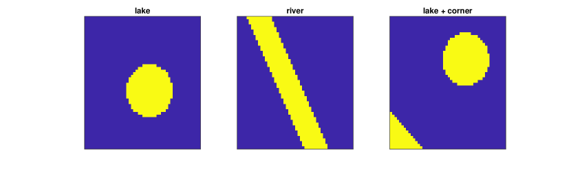
Figure 1: Test functions for propensity map ${\boldsymbol{\mu}}_{0}$

We generate an entire population of $n_{0}=5000$ individuals moving over a square fenced area $\Omega_{0}$ made of $N_{0}\times N_{0}$ lattice with known propensity ${\boldsymbol{\mu}}_{0}$ given by one of the three binary profiles in Figure 1 which simulates (from left to right) a lake, a river or a lake plus a corner. We choose a full discretization with $N_{0}=50$ to provide a fine mapping of the area. For individual $i\in\{1,\ldots,n_{0}\}$, we simulate $T=2880$ random moves $l^{(i)}_{1},l^{(i)}_{2},\cdots,l^{(i)}_{T}$ on the lattice $\Omega$. The value of $T=2880$ mimics GPS samplings every $t=15$ minutes for 30 days. At each time, the proposed moves are either to stay at the current location or to move to one of its four neighbors. We simulate two different herd behaviors: one half of the individuals moves randomly with equal probability $1/5$ to one of the five proposed moves, while the other half moves with a probability that depends on ${\boldsymbol{\mu}}_{0}$ in a way that doubles the probability of moving to a region of higher virus infection propensity. We call $L_{0}$ the $n_{0}\times T$ matrix which entry $(i,j)$ corresponds to the lattice locations of the $i$-th individual at time $t$. Based on $L_{0}$, we build the $n_{0}\times p_{0}$ matrix $X_{0}$ which counts the time spent in each of the $p_{0}=N_{0}^{2}$ lattice locations of $\Omega$ for each of the $n_{0}$ individuals. Then we generate the binary infection vector ${\bf y}_{0}$ whether the animal was infected during the time period, according to model (1). We expect more ones in the entries of ${\bf y}_{0}$ corresponding to the second herd which tends to stay in a region of higher virus infection propensity.

To investigate the impact of the spatial discretization of $\Omega_{0}$, we disctretize it into $(N\times N)$ lattices with $N\in\{10,30,50\}$, the largest $N$ corresponding to the full $\Omega_{0}$ plotted in Figure 1. To investigate the impact of different frequencies of the tracers placed on the individuals, we sample the $L_{0}$ matrix every $t\in\{1,96,480\}$ units, a unit being 15 minutes, which means that each tracer sends its current location either every 15 minutes, 24 hours or 120 hours (5 days). The corresponding matrix $L_{t}$ of GPS locations built from taking every $t$ columns of $L_{0}$ has $2880$, $720$ or $120$ columns, leading to a regression matrix $X$ of size $n_{0}\times p$, where $p=N^{2}$. Finally the number of tracers placed on the full population, that is, the number of observations, is taken as $n\in\{500,2000,5000\}$, the largest $n$ corresponding to the full population $n_{0}=5000$.

3.2 Propensity map estimation

We perform Monte Carlo simulations for each combination of the three propensity maps ${\boldsymbol{\mu}}_{0}$ plotted in Figure 1, the three spatial discretization $N\in\{10,30,50\}$, the three temporal frequencies $t\in\{1,4,24\}$ and the three sample sizes $n\in\{500,2000,5000\}$. Each scenario is simulated 100 times, leading to 100 full data information triplets $({\bf y}_{0},L_{0},X_{0})$, from which a response vector ${\bf y}$ is extracted and a regression matrix $X$ is built, depending on the value of $(N,t,n)$. For each ot the 100 data sets generated, we estimate the propensity map with our total variation estimator solution to (2) with the quantile universal threshold of Definition 1 for the value of $\lambda$. For comparison we also estimate the propensities using two approaches: a GLM fit with no total variation regularization (possible only when $n\geq p$, otherwise an infinite number of GLM exists) and a naive approach based on percentage of occupation by sick animals, namely

$$\hat{\mu}^{\rm naive}_{l}=\frac{\sum_{\{i|y_{i}=1\}}X_{i,l}}{\sum_{i=1}^{n}X_{i,l}},\quad l=1,\ldots,p.$$ (5)

Owing to the different values of $(N,t,n)$, we scale both the total variation, the un-regularized GLM and the naive method on the interval $[0,1]$ to compare them in terms of mean squared error calculated as ${\rm MSE}=\sum_{l=1}^{p}(\hat{\mu}_{l}-\tilde{\mu}_{0,l})^{2}/p$, where $\tilde{\boldsymbol{\mu}}_{0}$ is the nearest neighbor interpolation of ${\boldsymbol{\mu}}_{0}$ on a coarser scale and $p=N^{2}$. Table 2 reports the MSEs between $\hat{\boldsymbol{\mu}}$ and $\tilde{\boldsymbol{\mu}}_{0}$ averaged over the 100 Monte Carlo runs. Figures 2, 3, and 4 show typical estimations for the three propensity maps considered. We observe that our method outperforms the naive estimation in almost all scenarios. As expected, we also see that MSE decreases for the asymptotic we considered, namely when the spatial discretization $N$ increases, the GPS frequency $1/t$ increases and the sample size $n$ of individuals increases.

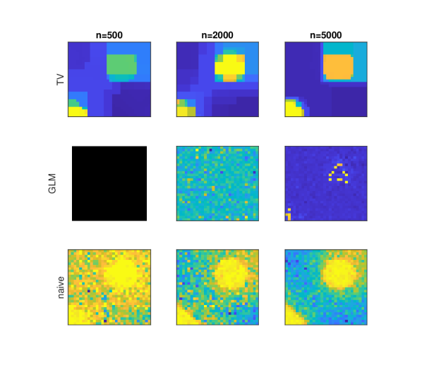
Figure 2: Examples of estimated lake + corner propensity maps for increasing sample sizes $n\in\{500,2000,5000\}$ (column-wise) and for the three TV, GLM and naive estimators (row-wise) for $(t,N)=(96,30)$.

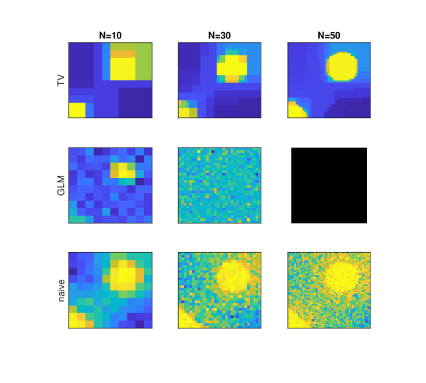
Figure 3: Estimated lake + corner propensity maps for increasing discretization indices $N\in\{10,30,50\}$ (column-wise), for the TV, GLM and naive estimators (row-wise) and for fixed $(t,n)=(96,2000)$.

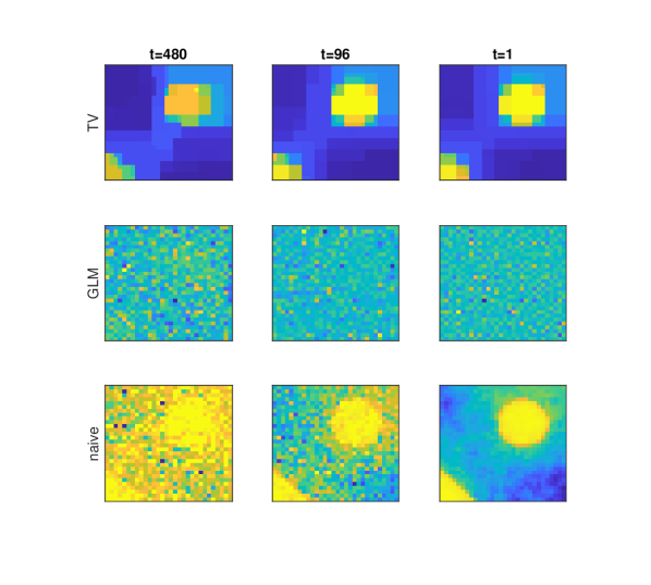
Figure 4: Estimated lake + corner propensity maps for increasing frequency $1/t$ with $t\in\{480,96,1\}$ (column-wise), for the TV, GLM and naive estimators (row-wise) and for fixed $(n,N)=(2000,30)$.

Table 2: Results of Monte Carlo simulation reporting the averaged mean squared errors between $\hat{\boldsymbol{\mu}}$ and ${\boldsymbol{\mu}}_{0}$ over 100 runs, for three estimators $\hat{\boldsymbol{\mu}}$ (TV, GLM and naive; best of three in bold), for the three propensity maps ${\boldsymbol{\mu}}_{0}$ (${\tt lake}$, ${\tt river}$ and ${\tt lake+corner}$) and for combinations of $(N,t,n)$.

		Estimated MSE
		$n=$	$500$	$2000$	$5000$		$500$	$2000$	$5000$		$500$	$2000$	$5000$
N	$t$		lake				river				lake+corner
$10$	480	TV	0.366	0.258	0.224		0.627	0.556	0.470		0.406	0.355	0.309
		GLM	0.318	0.284	0.236		0.374	0.389	0.284		0.329	0.326	0.255
		naive	0.545	0.428	0.395		0.595	0.510	0.487		0.566	0.451	0.412
	96	TV	0.299	0.218	0.190		0.606	0.514	0.418		0.382	0.316	0.255
		GLM	0.337	0.258	0.229		0.413	0.309	0.270		0.367	0.278	0.251
		naive	0.447	0.377	0.364		0.521	0.476	0.463		0.462	0.403	0.382
	1	TV	0.303	0.215	0.190		0.597	0.510	0.408		0.378	0.309	0.249
		GLM	0.371	0.292	0.256		0.452	0.337	0.300		0.412	0.319	0.279
		naive	0.426	0.362	0.356		0.503	0.467	0.460		0.439	0.389	0.376
$30$	480	TV	0.193	0.162	0.178		0.379	0.292	0.460		0.270	0.209	0.268
		GLM		0.506	0.313			0.527	0.384			0.510	0.346
		naive	0.771	0.734	0.625		0.793	0.757	0.669		0.784	0.747	0.641
	96	TV	0.166	0.149	0.122		0.367	0.371	0.392		0.233	0.194	0.214
		GLM		0.493	0.330			0.498	0.407			0.488	0.359
		naive	0.710	0.540	0.462		0.736	0.611	0.548		0.729	0.565	0.492
	1	TV	0.164	0.149	0.120		0.362	0.35	0.38		0.231	0.193	0.205
		GLM		0.507	0.469			0.521	0.487			0.508	0.462
		naive	0.467	0.372	0.348		0.544	0.481	0.463		0.480	0.401	0.373
$50$	480	TV	0.202	0.155	0.152		0.414	0.307	0.280		0.286	0.206	0.187
		GLM			0.502				0.514				0.502
		naive	0.792	0.760	0.712		0.796	0.782	0.733		0.797	0.773	0.720
	96	TV	0.160	0.126	0.128		0.395	0.265	0.245		0.236	0.171	0.156
		GLM			0.509				0.508				0.507
		naive	0.750	0.630	0.529		0.775	0.667	0.598		0.766	0.642	0.548
	1	TV	0.150	0.116	0.121		0.391	0.253	0.235		0.233	0.161	0.149
		GLM			0.520				0.516				0.521
		naive	0.491	0.309	0.359		0.559	0.485	0.461		0.511	0.414	0.379

3.3 Power of the TV-test for $H_{0}:{\boldsymbol{\mu}}=\mu_{0}{\bf 1}$ under a smooth alternative

We evaluate with a Monte Carlo simulation the power of the TV-test of Section 2.3 as a function of the sample size $n$ under the fixed alternative hypothesis that the propensity is the lake+corner map. Figure 5 reports the level (left plot) and the power (right plot) of four tests: the TV-test (4) and the LASSO-test (Sardy et al., 2022), the likelihood ratio test based on the asymptotic $\chi^{2}$ distribution, and the exact likelihood ratio test.

As far as level is concerned (here $\alpha=0.05$), one observes that the likelihood ratio test using the asymptotic $\chi^{2}$ distribution is far from its nominal level when $n$ is small. Not based on asymptotic, the other three tests achieve near nominal level (thanks to a Monte Carlo simulation to evaluate empirically the distribution of their respective test statistics under the null).

As far as power is concerned, the right plot of Figure 5 reveals that under an alternative hypothesis with spatial coherence like the lake+corner map, the TV-test is more powerful than the exact likelihood ratio test and the LASSO-test. The latter would be more powerful under a sparse alternative hypothesis since the LASSO penalty helps detect sparsity and the TV penalty helps detect spatial coherence.

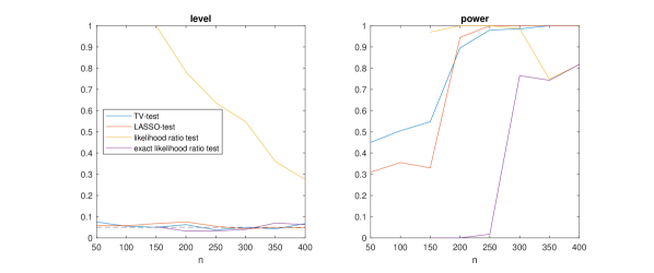
Figure 5: Plots of the level (left) and of the power (right) of four tests as a function of sample size $n$: TV-test, LASSO-test, the likelihood ratio test based either on the asymptotic $\chi^{2}$ distribution or on the exact distribution empirically sampled.

4 Application to white-tailed deer (WTD) data

We now apply the current model to the WTD data collected in a privately owned ranch in Florida. Details about number of individuals and specific data description have been provided in Section 1.1. We pre-processed the raw data to only keep GPS tracks that were sampled during similar periods and similar durations between blood tests. We excluded GPS tracks of seropositive individuals at both collection times because these individuals were infected prior to tracking. GPS tracks were interpolated to a minimum of 15 minutes. This resulted in 27 tracks for EHDV-1, 22 for EHDV-2, and 30 for EHDV-6, with average length of 14134, 14089, and 14159 geographical locations, respectively (see Table 1). To improve statistical power of the TV-test (see Section 3.3), each observed GPS track was resampled uniformly without replacement to generate tracks of 2000 locations. This procedure was repeated 20 times per interpolated GPS track to construct a data set consisting of 540, 480 and 600 tracks, respectively. Our data augmentation procedure generates spatially correlated tracks, mimicking the gregarious behavior of herds. Details on the code for the augmentation procedure and the resulting matrices $X$ and vectors $y$ are available in Section 6.

Figure 6 plots the three estimated propensity maps for the three serotypes (left column). Our method identified the southwestern area of the ranch as having the higher disease risk for EHDV-1. For EHDV-2, the method suggests that almost the entire study area is of high risk except for a small area around a feeder in the north central area. Such result might be due to a more widespread movement of the animals infected with EHDV-2 that with other serotypes. Interestingly no or very few infected animals visited a single feeder in the north central area of the ranch. This pattern merits further investigation to understand the underlying causes of this potential refuge. For EHDV-6 the eastern portion is also identified as a high risk area in addition to a specific pixel in the north eastern section of the ranch. Moreover, none of the models for EDHV-1 or EHDV-6 predicted the northwestern portion of the ranch as high risk. This results can be interpreted relative to the distribution and abundance of Culicoides across the ranch (right column). Relative abundance of C. stellifer, a candidate vector for EHDV transmission, was highest in the eastern section of the ranch. In contrast, the abundance of C. haematopotus was highest in the northeastern section. C. stellifer is a competent vector of EHDV for WTD while C. haematopotus primarily feeds on birds and not Cervids. Our model allowed us to identify higher risks in sections where there was a higher abundance of biting midge species, without any information about it, specifically.

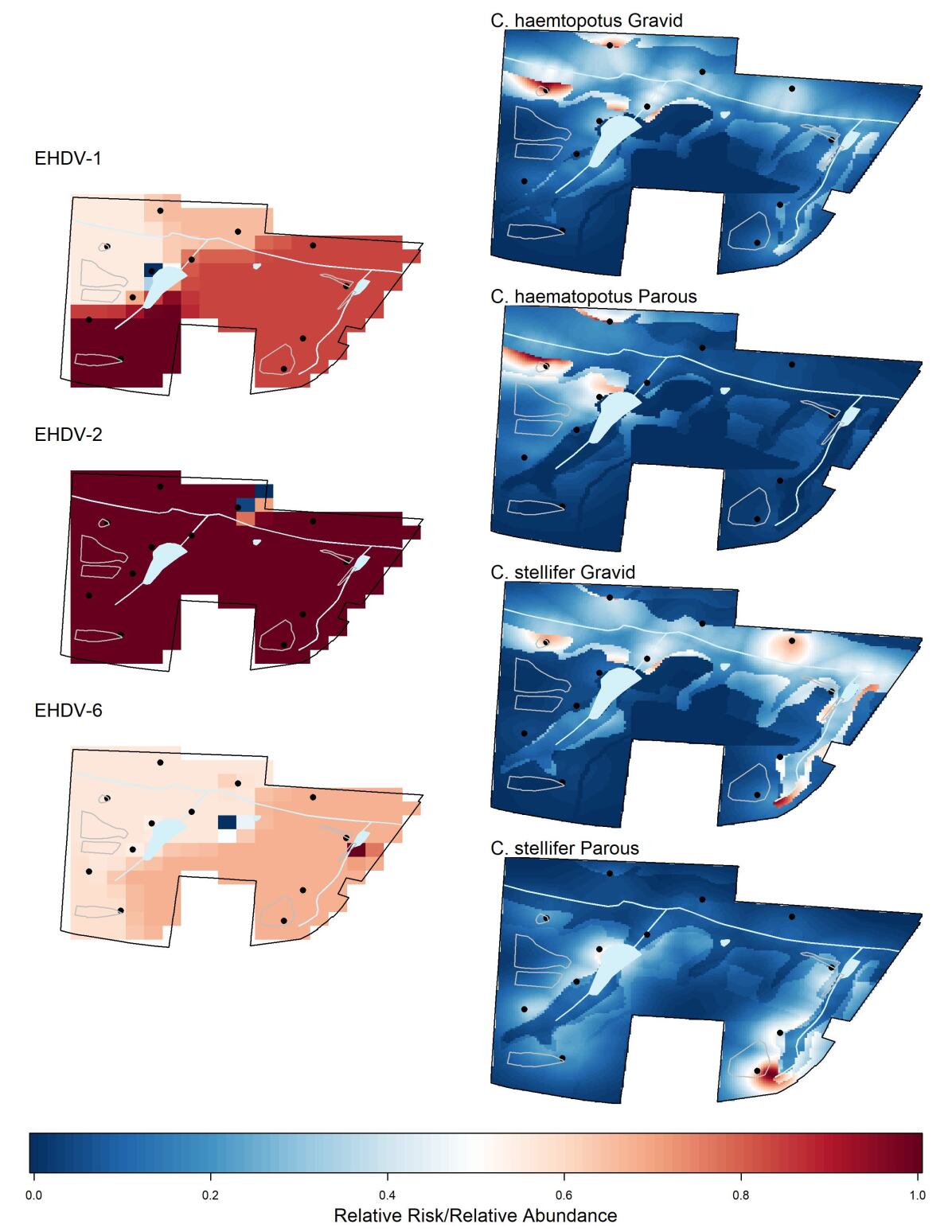
Figure 6: EHDV-1, EHDV-2 and EHD-6 disease risk estimation in white tailed deer and three exotic Cervid species in a ranch in north central Florida. The left column panels show the relative disease risk for each of the three serotypes evaluate based on TV model. Warmer colors show higher risk of getting infected. The right panels show the average relative abundance of Culicoides heamotopotus and Culicoides stellifer in week 14 of 2015 and 2016. C. stellifer is a competent vector of EHDV for WTD while C. haematopotus primarily feeds on birds and not Cervids.

5 Conclusion

Spatial epidemiologists and disease ecologists have used a wide variety of methods to predict disease risk. Current approaches integrate spatial analyses of infections, with host movement data and vector abundance. In all cases, there is a need for large amounts of movement, habitat selection, disease prevalence, environmental or vector abundance data and previous disease knowledge to make inferences about transmission risk. Our model was able to identify transmission risk without any prior knowledge on the abundance or ecology of biting midge species and environmental variables. This means, it can be used as a first approximation to predict disease risk and generate hypothesis about the ecology of infectious diseases without the need of having previous knowledge about the infection or its dynamics. This is a powerful tool to identify areas that need intervention to control emerging diseases with little epidemiological and ecological knowledge. We have shown, using WTD movement data, that our model predictions of EHDV risk are in line with previous knowledge about the ranch and vector abundance and ecology. The fact that the model identifies areas of low disease risk to be areas in which the abundant vector does not feed on Cervid species is an indication of the usefulness of this method.

One caveat of our method is that it requires recapturing individuals, which might prove challenging for some species. The sample size required and the time series length will depend on the geographical extent, ecology of the disease and movement ecology of the animals. Thus, although our model is completely naive regarding disease ecology, it is still important to have previous knowledge about host, vector and disease ecology to make decisions about the extent of the conclusions and adequate sample size. Nonetheless, for some animal groups, such as birds, recapturing individuals is a widely used technique for abundance and population dynamics estimation. It is well known that avian malaria presents a serious threat for bird populations Atkinson and Samuel (2010); Torres-Sorando and Rodriguez (1997), thus our method can be used to predict areas of high avian malaria risk or other diseases such as H1N1. We call for researchers studying movement ecology and population dynamics to consider incorporating the collection of serological status for particular diseases in order to populate the type of model we propose.

In this study, we introduce an innovative model that represents the inaugural application of a tomographic methodology to the estimation of landscape susceptibility to various risks, leveraging GPS signals from vectors in a manner analogous to the utilization of tomographic techniques in Positron Emission Tomography (PET) scans. Our model posits that by applying tomographic principles to analyze GPS data, it is possible to indirectly assess a range of risks associated with different landscapes. This approach not only broadens the applicability of tomography beyond its conventional medical context but also offers a novel perspective on risk estimation by harnessing the spatial data provided by vectors. We posit that our methodology holds significant potential for enhancing the precision and depth of landscape risk assessments, thereby contributing to the fields of geography, risk management, and spatial analysis.

6 Reproducible research

The code and data that generated the figures in this article may be found online at https://github.com/jairoadiazr/TVqut

Appendix A Proof of Property 1

The negative log-likelihood associated to model (1) is

$$h({\boldsymbol{\mu}};{\bf y}):=-\log{\rm L}(g^{-1}(X{\boldsymbol{\mu}});{\bf y})=\sum_{i=1}^{n}y_{i}\log(1+\exp(-{\bf x}_{i}^{\rm T}{\boldsymbol{\mu}})+\sum_{i=1}^{n}(1-y_{i})\log(1+\exp({\bf x}_{i}^{\rm T}{\boldsymbol{\mu}})).$$ (6)

Let $D$ be the $q\times p$ matrix of the $q$ finite differences such that $\|D{\boldsymbol{\mu}}\|_{1}=\sum_{l=1}^{p}\sum_{l^{\prime}\in\partial l}|\mu_{l}-\mu_{l^{\prime}}|$. Since all differences between neighbors are penalized and there are more finite differences than elements in the partition of $\Omega$ (that is, $q>p$), the kernel of $D$ is spanned by the constant vector. Moreover the cost function (2) is continuous in ${\boldsymbol{\mu}}$ and defined on ${\mathbb{R}}^{p}$, a closed set. The function $h$ is bounded from below by zero and the penalty term tends to infinity unless ${\boldsymbol{\mu}}$ is in the kernel of $D$. Since all entries of X are positive (they are total times) and each row of $X$ has at least one strictly positive entry (an animal is part of the study if he spent some time in the ranch), the entries of $X{\bf 1}$ are strictly positive; consequently, it is easy to check that $\lim_{\epsilon\rightarrow\pm\infty}h(\epsilon{\bf 1};{\bf y})=+\infty$ under the assumption the entries of ${\bf y}$ are not all ones or all zeros. So the cost function (2) is coercive. Weierstrass theorem guarantees a minimum in ${\mathbb{R}}^{p}$ for any given $\lambda>0$.

The cost function (2) is moreover convex, and the Lagrange function associated to it is

$${\cal L}({\boldsymbol{\mu}},{\boldsymbol{\gamma}},{\boldsymbol{\omega}})=h({\boldsymbol{\mu}};{\bf y})+\lambda\|{\boldsymbol{\gamma}}\|_{1}+{\boldsymbol{\omega}}^{\rm T}(D{\boldsymbol{\mu}}-{\boldsymbol{\gamma}}).$$

So the Lagrangian dual problem of (2) is

$$\max_{\|{\boldsymbol{\omega}}\|_{\infty}\leq\lambda}\min_{\boldsymbol{\mu}}h({\boldsymbol{\mu}};{\bf y})+{\boldsymbol{\mu}}^{\rm T}D^{\rm T}{\boldsymbol{\omega}}.$$

Consequently there exists a finite $\lambda$ that leads to the constant MLE estimate, given by

$$\min_{{\boldsymbol{\omega}}\in{\mathbb{R}}^{q}}\|{\boldsymbol{\omega}}\|_{\infty}\quad{\rm s.t.}\quad\nabla_{\boldsymbol{\mu}}h({\boldsymbol{\mu}};{\bf y})+D^{\rm T}{\boldsymbol{\omega}}={\bf 0},\ {\boldsymbol{\mu}}=\hat{\beta}_{0}{\bf 1},\ \hat{\beta}_{0}=\operatorname*{\arg\!\min}_{\beta_{0}}h(\beta_{0}{\bf 1};{\bf y}).$$

References

- Ahmed et al. [2015] S. Ahmed, G. Mcinerny, K. O’Hara, R. Harper, L. Salido, S. Emmott, and L. Joppa. Scientists and software - surveying the species distribution modeling community. Diversity and Distributions, 21, 03 2015.
- Albery et al. [2022] G. Albery, A. Sweeny, D. Becker, and S. Bansal. Fine-scale spatial patterns of wildlife disease are common and understudied. Functional Ecology, 36(1):214–225, 2022.
- Atkinson and Samuel [2010] C. Atkinson and M. Samuel. Avian malaria plasmodium relictum in native hawaiian forest birds: epizootiology and demographic impacts on apapane himatione sanguinea. Journal of Avian Biology, 41(4):357–366, 2010.
- Brdar et al. [2016] S. Brdar, K. Gavrić, D. Ćulibrk, and V. Crnojević. Unveiling spatial epidemiology of hiv with mobile phone data. Scientific reports, 6(1):19342, 2016.
- Bühlmann and van de Geer [2011] P. Bühlmann and S. van de Geer. Statistics for High-Dimensional Data: Methods, Theory and Applications. Springer, Heidelberg, 2011.
- Cauvin et al. [2020] A. Cauvin, E. Dinh, J. Orange, R. Shuman, J. Blackburn, and S. Wisely. Antibodies to epizootic hemorrhagic disease virus (ehdv) in farmed and wild florida white-tailed deer (odocoileus virginianus). Journal of wildlife diseases, 56(1):208–213, 2020.
- de Thoisy et al. [2020] B. de Thoisy, N. Silva Oliveira, L. Sacchetto, G. de Souza Trindade, and B. Drumond. Spatial epidemiology of yellow fever: Identification of determinants of the 2016-2018 epidemics and at-risk areas in brazil. PLoS neglected tropical diseases, 14(10):e0008691, 2020.
- Dinh et al. [2020] E. Dinh, A. Cauvin, J. Orange, R. Shuman, S. Wisely, and J. Blackburn. Living la vida t-locoh: Site fidelity of florida ranched and wild white-tailed deer (odocoileus virginianus) during the epizootic hemorrhagic disease virus (ehdv) transmission period. Movement ecology, 8:1–9, 2020.
- Dinh et al. [2021a] E. Dinh, J. Gomez, J. Orange, M. Morris, K. Sayler, B. McGregor, E. Blosser, N. Burkett-Cadena, S. Wisely, and J. Blackburn. Modeling abundance of culicoides stellifer, a candidate orbivirus vector, indicates nonrandom hemorrhagic disease risk for white-tailed deer (odocoileus virginianus). Viruses, 13(7):1328, 2021a.
- Dinh et al. [2021b] E. Dinh, J. Orange, R. Peters, S. Wisely, and J. Blackburn. Resource selection by wild and ranched white-tailed deer (odocoileus virginianus) during the epizootic hemorrhagic disease virus (ehdv) transmission season in florida. Animals, 11(1):211, 2021b.
- Dougherty et al. [2018] E. Dougherty, D. Seidel, C. Carlson, O. Spiegel, and W. Getz. Going through the motions: incorporating movement analyses into disease research. Ecology letters, 21(4):588–604, 2018.
- Dougherty et al. [2022] E. Dougherty, D. Seidel, J. Blackburn, W. Turner, and W. Getz. A framework for integrating inferred movement behavior into disease risk models. Movement ecology, 10(1):1–15, 2022.
- Elith et al. [2011] J. Elith, S. Phillips, T. Hastie, M. Dudik, Y. Chee, and C. Yates. A statistical explanation of maxent for ecologists. Diversity and Distributions, 17(1):43–57, 2011.
- Estrada-Pena et al. [2014] A. Estrada-Pena, R. Ostfeld, A. Peterson, R. Poulin, and J. De la Fuente. Effects of environmental change on zoonotic disease risk: An ecological primer. Trends in parasitology, 30, 03 2014.
- Frias-Martinez et al. [2012] V. Frias-Martinez, A. Rubio, and E. Frias-Martinez. Measuring the impact of epidemic alerts on human mobility using cell-phone network data. In Second Workshop on Pervasive Urban Applications@ Pervasive, volume 12, 2012.
- Giacobino et al. [2017] C. Giacobino, S. Sardy, J. Diaz-Rodriguez, and N. Hengardner. Quantile universal threshold. Electronic Journal of Statistics, 11:4701–4722, 2017.
- Harvell et al. [2002] C. Harvell, C. Mitchell, J. Ward, S. Altizer, A. Dobson, R. Ostfeld, and M. Samuel. Climate warming and disease risks for terrestrial and marine biota. Science (New York, N.Y.), 296:2158–62, 07 2002.
- Hollingsworth et al. [2015] T. Hollingsworth, J. Pulliam, S. Funk, J. Truscott, V. Isham, and A. Lloyd. Seven challenges for modelling indirect transmission: Vector-borne diseases, macroparasites and neglected tropical diseases. Epidemics, 10, 08 2015.
- Keeling et al. [2008] M. Keeling, P. Rohani, and B. Pourbohloul. Modeling infectious diseases in humans and animals. Clinical infectious diseases : an official publication of the Infectious Diseases Society of America, 47:864–865, 10 2008.
- Killilea et al. [2008] M. Killilea, A. Swei, R. Lane, C. Briggs, and R. Ostfeld. Spatial dynamics of lyme disease: A review. EcoHealth, 5:167–95, 07 2008.
- Kirby et al. [2017] R. Kirby, E. Delmelle, and J. Eberth. Advances in spatial epidemiology and geographic information systems. Annals of Epidemiology, 27, 12 2017.
- Lima et al. [2015] A. Lima, M. De Domenico, V. Pejovic, and M. Musolesi. Disease containment strategies based on mobility and information dissemination. Scientific reports, 5(1):1–13, 2015.
- McGregor et al. [2019a] B. McGregor, K. Sloyer, K. Sayler, O. Goodfriend, J. Krauer Campos, C. Acevedo, X. Zhang, D. Mathias, S. Wisely, and N. Burkett-Cadena. Field data implicating culicoides stellifer and culicoides venustus (diptera: Ceratopogonidae) as vectors of epizootic hemorrhagic disease virus. Parasites & vectors, 12:1–13, 2019a.
- McGregor et al. [2019b] B. McGregor, T. Stenn, K. Sayler, E. Blosser, J. Blackburn, S. Wisely, and N. Burkett-Cadena. Host use patterns of culicoides spp. biting midges at a big game preserve in florida, usa, and implications for the transmission of orbiviruses. Medical and veterinary entomology, 33(1):110–120, 2019b.
- Messina et al. [2015] J. Messina, O. Brady, D. Pigott, N. Golding, M. Kraemer, T. Scott, W. Wint, D. Smith, and S. Hay. The many projected futures of dengue. Nature Reviews Microbiology, 13:230–239, 04 2015.
- Morris and Blackburn [2016] L. Morris and J. Blackburn. Predicting disease risk, identifying stakeholders, and informing control strategies: A case study of anthrax in montana. EcoHealth, 13(2):262–273, Jun 2016.
- Nelder and Wedderburn [1972] J. A. Nelder and R. W. M. Wedderburn. Generalized linear models. Journal of the Royal Statistical Society: Series A, 135(3):370–384, 1972.
- Orange et al. [2021a] J. Orange, E. Dinh, O. Goodfriend, S. Citino, S. Wisely, and J. Blackburn. Evidence of epizootic hemorrhagic disease virus and bluetongue virus exposure in nonnative ruminant species in northern florida. Journal of Zoo and Wildlife Medicine, 51(4):745–751, 2021a.
- Orange et al. [2021b] J. Orange, E. Dinh, R. Peters, S. Wisely, and J. Blackburn. Inter-annual home range fidelity of wild and ranched white-tailed deer in florida: implications for epizootic hemorrhagic disease virus and bluetongue virus intervention. European Journal of Wildlife Research, 67:1–8, 2021b.
- Ostfeld et al. [2005] R. Ostfeld, G. Glass, and F. Keesing. Spatial epidemiology: an emerging (or re-emerging) discipline. Trends in Ecology and Evolution, 20(6):328 – 336, 2005.
- Patz et al. [2008] J. A Patz, S. H. Olson, C. K. Uejio, and H. K. Gibbs. Disease emergence from global climate and land use change. Medical Clinics of North America, 92(6):1473–1491, 2008.
- Ragg and Moller [2000] J. Ragg and H. Moller. Microhabitat selection by feral ferrets (mustela furo) in a pastoral habitat, east otago, new zealand. New Zealand Journal of Ecology, pages 39–46, 2000.
- Riley et al. [2015] S. Riley, K. Eames, V. Isham, D. Mollison, and P. Trapman. Five challenges for spatial epidemic models. Epidemics, 10:68 – 71, 2015. Challenges in Modelling Infectious Disease Dynamics.
- Rudin et al. [1992] L. I. Rudin, S. Osher, and E. Fatemi. Nonlinear total variation based noise removal algorithms. Physica D, 60:259–268, 1992.
- Sardy and Monajemi [2019] S. Sardy and H. Monajemi. Efficient threshold selection for multivariate total variation denoising. Journal of Computational and Graphical Statistics, 28(1):23–35, 2019.
- Sardy et al. [2022] S. Sardy, J. Diaz-Rodriguez, and C. Giacobino. Thresholding tests based on affine lasso to achieve non-asymptotic nominal level and high power under sparse and dense alternatives in high dimension. Comput. Stat. Data Anal., 173(C), 2022.
- Stallknecht et al. [1996] D. Stallknecht, M. Luttrell, K. Smith, and V. Nettles. Hemorrhagic disease in white-tailed deer in texas: a case for enzootic stability. Journal of wildlife Diseases, 32(4):695–700, 1996.
- Stockwell [1999] D. Stockwell. The garp modelling system: problems and solutions to automated spatial prediction. International journal of geographical information science, 13(2):143–158, 1999.
- Tibshirani [1996] R. Tibshirani. Regression shrinkage and selection via the lasso. Journal of the Royal Statistical Society, Series B, 58(1):267–288, 1996.
- Torres-Sorando and Rodriguez [1997] L. Torres-Sorando and D. Rodriguez. Models of spatio-temporal dynamics in malaria. Ecological Modelling, 104(2):231 – 240, 1997.