Contact-based molecular dynamics of structured and disordered proteins in a coarse-grained model: fixed contacts, switchable contacts and those described by pseudo-improper-dihedral angles

Abstract

We present a coarse-grained C_α-based protein model that can be used to simulate structured, intrinsically disordered and partially disordered proteins. We use a Go-like potential for the structured parts and two different variants of a transferable potential for the disordered parts. The first variant uses dynamic structure-based (DSB) contacts that form and disappear quasi-adiabatically during the simulation. By using specific structural criteria we distinguish sidechain-sidechain, sidechain-backbone and backbone-backbone contacts. The second variant is a non-radial multi-body pseudo-improper-dihedral (PID) potential that does not include time-dependent terms but requires more computational resources. Our model can simulate in reasonable time thousands of residues on millisecond time scales.

PROGRAM SUMMARY

Program Title: cg
Licensing provisions: MIT
Programming language: C++ (new version), Fortran (old version)
Nature of problem(approx. 50-250 words):

Simulations of one or more protein chains, structured, intrinsically disordered or partially disordered. Calculating their equilibrium and kinetic properties in processes including but not limited to: folding, aggregation, conformational changes, formation of complexes, aggregation, response to deformation. All those processes need long simulation times or many trajectories to properly sample the system.

Solution method(approx. 50-250 words):

The simulations use a molecular dynamics implicit-solvent coarse-grained model where each pseudoatom represents one amino acid residue. Residues are harmonically connected to form a chain. The system evolves according to Langevin dynamics. The backbone stiffness potential involves bond angle and dihedral angle terms (or a chirality term in the structured case). Residues interact via modified Lennard-Jones or Debye-Hueckel potentials.

The potential is different for structured and disordered parts of a protein. A Go model contact map is used for the structured parts, where an interaction between two residues is attractive if effective spheres associated with their heavy atoms overlap in the native structure [1,2,3,4]. Non-attractive contacts use only the repulsive part of the Lennard-Jones potential. The potential for the disordered parts has two versions: in the quasi-adiabatic Dynamic Structure-Based (DSB) variant, the contacts are formed dynamically based on the structure of the chain and are quasi-adiabatically turned on and off [5,6]. In the slower, but more accurate Pseudo-Improper-Dihedral (PID) variant the Lennard-Jones term is multiplied by a pseudo-improper-dihedral term that gives similar geometric restrictions with a time-independent Hamiltonian [7].

Proteins can be pulled by their termini to mimic stretching by an Atomic Force Microscope [8,9]. Multiple protein chains can be put in a simulation box with periodic boundary conditions or with walls that may be repulsive or attractive for the residues. The walls may move to mimic pulling or shearing deformations. The program accepts PDB files or protein sequences with optional user-defined contact maps. It saves the results in an output file (summary), a PDB file (structure) and a map file (contact map in a given snapshot).

Additional comments including Restrictions and Unusual features (approx. 50-250 words):
The program supports openMP (effective up to 8 cores, use 4 cores for optimal speed-up). The C++ version is hosted on Github, the Fortran version is distributed as a .tar archive.

1 Usage

There are two versions of the program: in C++ (new) and in FORTRAN (old). They should give the same results (up to numerical accuracy), with the exception of boundary conditions in the form of a simulation box with attractive walls (see section 5.1.5). The C++ version is well documented online (https://vitreusx.github.io/pas-cg/). The rest of this paper refers to the old, Fortran version.

The program is a single FORTRAN file (cg.f). After compilation, it requires exactly one argument: the name of the inputfile. Names of all the other files that may be needed must be written in the inputfile. Possible input and output files are shown in Fig. 1. All files used in the program are in the plain text format. Each line of the inputfile has two words separated by a single space: the name of a variable and the value it should have. All variables have a predefined default value, so only the non-default variables need to be included in the inputfile. More technical details (like the list of the variables) are summarized in the README.txt file. This program is distributed as a .tar archive.

Figure 1: A scheme visualizing the usage of the program.

2 Equations of motion

Each pseudoatom is centered at the position of the C_α atom of the amino acid it represents. We use Langevin dynamics with the following equation of motion for the $i$-th residue in a chain:

$$m\frac{d^{2}\vec{r}_{i}}{d^{2}t}=\vec{F}_{i}-\gamma\frac{d\vec{r}_{i}}{dt}+\vec{\Gamma_{i}}$$ (1)

where $m$ is the average amino acid mass (the variable lmass allows to turn on different amino acid masses), $\vec{r}_{i}$ is the position of the residue, $\vec{F}_{i}$ is the force resulting from the potential, $\gamma=2m/\tau$ is the damping coefficient and $\vec{\Gamma_{i}}$ is the thermal white noise with the variance $\sigma_{T}^{2}=2\gamma k_{B}T$. The implicit solvent is implemented via this noise and the damping. The default damping coefficient $\gamma=2m/\tau$ is chosen to represent an overdamped case with diffusional (not ballistic) dynamics. More realistic values of $\gamma$ should be about 25 times larger [1, 2], but adopting them would lead to a much longer conformational dynamic.

The time unit $\tau\approx 1$ ns was verified for a different model with the same equations of motion [3], so the value of $\tau$ is only orientational. The equations of motion are integrated by the fifth order predictor-corrector algorithm [4, 5]. One $\tau$ corresponds to 200 integration steps.

The energy is expressed in units of $\epsilon$, where $\epsilon\approx 1.5$ kcal/mol [6, 7]. The internal unit of energy in the code is also $\epsilon$. The distances in the input and output of the program are in the units of Å. However, the distances used in the integrating module are dimensionless: they are divided by 5 Å; hence the conversion unit unit of 5. (so a distance ,,10 Å” in the input is processed as ,,2” during the integration of the equations of motion).

The residues in one chain are tethered harmonically with the spring constant $k=100$ Å${}^{-2}\cdot\epsilon$ and the equilibrium distance between them is taken as 3.8 Å. If the simulation is based on a PDB file, equilibrium distances are taken from that file and can be different from 3.8 Å. Due to limitations in the chain numbering in the PDB files, the program allows only 153 unique chain labels in a single file. However, there are ways to use more than one file [8, 9]. In Fortran, logical values true and false are denoted as T and F, respectively. Setting the variable lwritexyz to T causes the program to use a much simpler XYZ format, which does not distinguish between chains (and prints only the x,y,z positions of each residue).

3 Backbone stiffness

Local interactions between amino acids separated by at most three residues in the protein sequence are known to stabilize folded proteins and improve their folding kinetics [10], and are even more important in determining the conformational ensembles of disordered proteins [11]. Those local interactions require using special backbone stiffness potentials (although in this program residues $i$ and $j\geq i+3$ can also attract each other in non-local interactions). Below we describe those potentials. Unstructured parts of a chain can use only bond angle and dihedral angle terms.

3.1 Chirality potential for structured parts

Chirality potential is defined [12] as $V^{CH}=\frac{1}{2}e_{chi}\Sigma_{i=2}^{i=N-2}(C_{i}-C^{n}_{i})^{2}$ where $N$ is the number of residues and the chirality of the residue $i$ is $C_{i}=(\vec{v}_{i-1}\times\vec{v}_{i})\cdot\vec{v}_{i+1}/d_{0}^{3}$ where $\vec{v}_{i}=\vec{r}_{i+1}-\vec{r}_{i}$ and $d_{0}$ is equal to the length of $\vec{v}_{i}$ in the native structure (usually very close to 3.8 Å). $C^{n}_{i}$ is the chirality of residue $i$ in the native structure. This dependence on the native structure restricts usage of the chirality potential only to structured proteins (the variable lpdb must be set to T). This potential can be turned on by setting the variable lchiral to T. The amplitude $e_{chi}$ of the potential can be tuned using the variable echi (the default value is 1, in the internal units of energy $\epsilon\approx$ 110 pN$\cdot$Å). It is computationally faster than the backbone stiffness potential based on the bond and dihedral angle terms defined below, but it is important to note that using chirality potential (with the default echi) lowers the effective room temperature of the system to 0.25 (in the program units, which correspond to $\epsilon/k_{B}$). The room temperature for structured proteins corresponds to the minimum of the median folding time and other properties of the system, defined in [12].

3.2 Bond and dihedral angle potentials

The bond angle between residues $i-1,i,i+1$ is defined as $\theta_{i}$, and the dihedral angle between residues $i-2,i-1,i,i+1$ is $\phi_{i}$. Backbone stiffness potentials based on those angles are turned on by the variable langle.

3.2.1 Structured parts

The bond angle potential for the structured parts is harmonic with the minimum in the bond angle $\theta_{n}$ present in the native structure: $V_{\theta}=k_{\theta}(\theta-\theta_{n})^{2}$, where the value of $k_{\theta}$ is defined by the variable CBA (its default value is 30, in $\epsilon/$rad² units).

The bond angle term is usually used together with the dihedral term, which can be turned on by setting the variable ldih T. The dihedral term has two forms. If the variable ldisimp is set to T, the harmonic form is used: $V_{\phi}^{simp}=\frac{1}{2}k_{\phi}(\phi-\phi_{n})^{2}$, where $\phi_{n}$ is the dihedral angle in the native structure and $k_{\phi}$ can be set in the variable CDH (with the default value of 3.33, in $\epsilon/$rad² units). The room temperature for this set of parameters has not been determined.

When ldisimp is F, a more sophisticated dihedral potential is used: $V_{\phi}=K_{1}[1-\cos(\phi-\phi_{n})]+K_{3}[1-\cos(3(\phi-\phi_{n}))]$, where the $K_{1}$ and $K_{3}$ parameters are specified by variables CDA and CDB, both with a default value 0.66 (in $\epsilon/$rad² units), respectively. This set of values (together with the bond angle potential) corresponds to room temperature 0.7, at which the kinetics of folding of structured proteins is optimal [12].

3.2.2 Unstructured parts

For the backbone stiffness of the unstructured parts we use a 3-letter alphabet distinguishing Gly, Pro and X residues, where X is one of the 18 other amino acids. For the bond angle we check only what the second and third residues are in the three consecutive residues forming the angle, which gives 9 possible choices. Including the first residue would give 27 possibilities, but the symmetry between the first and the third residue in a bond angle can be broken (because proteins are chiral). The bond angle potential has the form of a sixth degree polynomial. Its coefficients for all 9 cases are listed in the parameter file specified by the variable paramfile.

The dihedral angle requires a consideration of four consecutive residues but we distinguish only the two central ones, which again gives 9 possible combinations. The dihedral potential is governed by a formula $a\sin(\phi)+b\cos(\phi)+c\sin^{2}(\phi)+d\cos^{2}(\phi)+e\sin(\phi)\cos(\phi)$, where the values of the coefficients $a,b,c,d,e$ for all 9 cases are also listed in the paramfile.

The coefficients for both the bond angle and the dihedral potentials were obtained [13] by fitting the formulas to a potential resulting from the inverse Boltzmann method applied to a random coil database. This potential was shown to correctly describe properties of proteins in denaturating conditions [14]. Thus our backbone stiffness has no preference towards any secondary structure, but $\alpha$-helices and $\beta$-sheets can still be formed by the backbone-backbone contacts (see section 4.2).

Ghavami et al [14] distinguished only the middle residue and whether it precedes proline, so only 6 from the 9 combinations in the paramfile are different.

The backbone stiffness is important in setting the effective room temperature for the model [12], so in this case we checked what temperature corresponds best to the experimental end-to-end distances for the polyprolines of various lengths [15]. We chose polyproline because its conformation is mostly determined by its backbone stiffness, so the parameters unrelated to the backbone stiffness could be optimized in the correct temperature. Temperatures between 0.35 and 0.4 $\epsilon/k_{B}$ turned out to be optimal, which is consistent with our energy unit $\epsilon\approx 1.5$ kcal/mol. Then 0.38 $\epsilon/k_{B}\approx 300$ K.

3.2.3 User-defined potential

The backbone stiffness potential may be also specified in a table where each row corresponds to a different angle and each column to a different Gly/Pro/X combination (in the same manner as in the previous section). The file stiffnesstabularized.txt contains the Boltzmann inversion potentials from Ghavami et al [14].

4 Non-local potential

The non-local potential is different for structured and disordered proteins. Possible variants of the potential together with the variables needed to switch between them are schematically shown in Fig. 2.

Figure 2: A scheme showing variants of the non-local potential.

4.1 Structured parts

If the variables lpdb and lallatom are set to T and a PDB file is provided, the program automatically constructs from the PDB file a contact map based on the overlap of heavy atoms [16] after assigning to each of them a radius that takes into account different positions of atoms in the amino acid (e. g. it distinguishes the radii of C_α and C_β atoms) [17]. In the case of an incomplete PDB file a simpler contact map based on C_α-C_α distances may be used (by setting lallatom F).

An analysis of 62 variants of the Go-like models has identified four that show the best agreement with the experimental stretching of structured proteins by means of tips mounted in the Atomic Force Microscopes (AFM). Among the four there is a simple variant in which each attractive contact is described by a Lennard-Jones (L-J) potential with the depth 1 $\epsilon$ [18].

It is important to note that the overlap of heavy atoms is just one possible criterion for defining a contact. More sophisticated criteria may involve the chemical identity of the overlapping heavy atoms [19]. Constructing such contact maps is not possible in the program presented here, but we provide a webserver for computing contact maps using a rCSU method: info.ifpan.edu.pl/~rcsu/

The simple L-J potential describing an attractive interaction between residues $i$ and $j$ has the form $\epsilon\left[{\left(\frac{r_{min^{ij}}}{r}\right)}^{12}-2\left(\frac{r_{min^{ij}}}{r}\right)^{6}\right]=4\epsilon\left[{\left(\frac{\sigma_{ij}}{r}\right)}^{12}-\left(\frac{\sigma_{ij}}{r}\right)^{6}\right]$, where $r_{min^{ij}}=2^{1/6}\sigma_{ij}$ is the minimum of the potential (for the structured proteins it is equal to the C_α-C_α distance in the native conformation). The residues that are not in a contact repel each other with a truncated and shifted form of the L-J potential: $V_{r}(r\leq r_{o})=\epsilon\left[{\left(\frac{r_{min}}{r}\right)}^{12}-2\left(\frac{r_{min}}{r}\right)^{6}+1\right]$, where $r_{o}=4$ Å  ensures the excluded volume (by default it is set to 5 Å  in the variable cut). Contacts between the $i$th and $i+2$nd residues are always described by the repulsive version of the L-J potential (also in potentials for disordered proteins). Please set cut to 4 Å when using only the structure-based potential, in order to get results consistent with the literature [6, 12, 18].

4.2 Unstructured parts

The backbone stiffness potential for disordered parts does not favor any secondary structure, so in order to make structures like $\alpha$-helices or $\beta$-sheets possible, we allow for attractive contacts between the $i$th and $i+3$rd residues in the chains, as these contacts correspond to hydrogen bonds between backbone atoms in the all-atom representation [20]. Forming backbone-backbone contacts results in helix-like and sheet-like structures that are similar to $\alpha$-helices and $\beta$-sheets (see Fig. 3). In this approximate way, our model incorporates secondary structure elements that may be disrupted and reformed, as backbone-backbone contacts keep being broken and reestablished. However the nature of $i,i+4$ contacts is different: the quasi-adiabatic potential works best with $i,i+4$ contacts turned on (the variable lii4 set to T), and the pseudo-improper-dihedral potential without them (lii4 F). A more detailed comparison of the model variants is available in [21].

The logical variable lcpot controls if our custom potential for disordered proteins is turned on. With lcpot F only residue pairs listed in the contact map attract each other. Setting lcpot T allows for a custom potential for all the residues, except those present in user-defined contact maps. So if you provide a PDB file and tell the program to construct a Go model contact map for it (by specifying lpdb T), but at the same time you set lcpot T, the pairs of residues listed in the contact map will interact via the ,,simple” L-J potential described above, but those not in the contact map will be subject to a potential customized for intrinsically disordered proteins. Therefore, the lcpot option should also be used for proteins that are only partially disordered. There are two versions of the disordered potential: quasi-adiabatic and pseudo-improper-dihedral. Both of them are described below.

4.2.1 Quasi-adiabatic potential

Figure 3: Three examples of conformations generated by the quasi-adiabatic potential [13].

The default, quasi-adiabatic version is faster, and uses contacts described by the L-J potential with the depth 1 $\epsilon$ (just as the Go potential for the structured parts) and a minimum $r_{min}$ (defined below), but here the contacts are formed and broken quasi-dynamically, based on the geometry of the chain. As real amino acids are made from a sidechain and a backbone, in our model we distinguish sidechain-sidechain (ss), backbone-sidechain (bs) and backbone-backbone (bb) contacts (each has different criteria for formation, but only one type of contact can be made between residues at a given time).

After conditions for forming the contact are met, formation of the contact happens quasi-adiabatically: the depth of the L-J potential well increases linearly form 0 to $\epsilon$ within 10$\;\tau$, which is long enough for the system to thermalize, but short enough to not disrupt dynamics of the system [13]. Breaking the contact also happens quasi-adiabatically, with the same time scale.

There are 3 criteria for forming a contact between residues $i$ and $j$:

• Distance: each type of contact has specific $r_{min}$ associated with it (based on a maximum of a statistical distribution from the PDB [13]). It is 5 Å  for bb, 6.8 Å  for bs, and a value specific for a given pair of amino acids for an ss contact. Those numbers are specified in the paramfile. To make a contact of a given type, the distance $r_{i,j}$ between the residues must be smaller than $r_{min}\cdot(1+tolerance)$ to make a contact (the default value of the variable tolerance is 0).

• Direction: the approximate directions of a backbone hydrogen bond or a sidechain C_β atom may be derived based on the position of 3 consecutive C_α atoms [22, 23, 13]. Let’s assume that $v_{i}$ is the vector connecting the $i$th and $i+1$st beads (centered on the supposed positions of the C_α atoms). Then we can construct two auxiliary vectors:

  $${\bf n}_{i}=\frac{{\bf v}_{i}-{\bf v}_{i-1}}{{\bf v}_{i}-{\bf v}_{i-1}} {\bf h}_{i}=\frac{{\bf v}_{i}\times{\bf v}_{i-1}}{|{\bf v}_{i}\times{\bf v}_{i-1}|}$$ (2)

  They represent the normal (${\bf n}_{i}$) and binormal (${\bf h}$) vectors of the Frenet frame defined by the ${\bf v}_{i},{\bf v}_{i-1}$ vectors, and can be associated with the direction of the sidechain ($-{\bf n}_{i}$) and with the direction of a hydrogen bond made by an atom from the backbone ($\pm{\bf h}_{i}$). A survey of the contacts from the PDB [22, 23] led to the following criteria for a contact of each type:

  • bb: $|cos({\bf{h}}_{i},{\bf{r}}_{i,j})|>0.92$, $|cos({\bf{h}}_{j},{\bf{r}}_{i,j})|>0.92$ (the threshold angle is 23^o), $|cos({\bf{h}}_{i},{\bf{h}}_{j})|>0.75$ (the treshold angle is 41^o)

  • bs: $\cos({\bf n}_{i},{\bf r}_{i,j})<0.5$, $|\cos({\bf h}_{j},{\bf r}_{j,i})|>0.92$ (where the $i$th residue donates its sidechain and the $j$th residue its backbone)

  • ss: $\cos({\bf n}_{i},{\bf r}_{i,j})<0.5$, $\cos({\bf n}_{j},{\bf r}_{j,i})<0.5$ (the threshold angle is $60^{o}$)

• Coordination number: the solvent in the program is implicit, so we cannot simulate how polar residues make contacts with water molecules. Using the one-bead-per-residue model also makes the protein less dense than it really is. We try to atone for that by allowing each amino acid to form only a limited number of contacts. Each residue can make only 2 contacts with their backbone (1 for proline) and $s$ ss contacts with their sidechain. Out of these contacts only $n_{H}$ can be made with hydrophobic residues and $n_{P}$ with polar residues. $s$, $n_{H}$ and $n_{P}$ depend on the amino acid. Those numbers and the division into polar and hydrophobic residues are available in the paramfile and here in the table 1. Those values are based on the PDB statistics [13]. bs contacts are considered to be ,,polar” (thus $n_{H}+n_{P}$ may be bigger than $s$).

  name	Gly	Pro	Gln	Cys	Ala	Ser	Val	Thr	Ile	Leu
  type	-	-	P	P	H	P	H	P	H	H
  $s$	0	0	2	3	3	2	4	2	5	5
  $n_{H}$	0	0	0	2	1	0	4	0	4	4
  $n_{P}$	0	0	2	2	1	2	1	2	2	2
  name	Asn	Asp	Lys	Glu	Met	His	Phe	Arg	Tyr	Trp
  type	P	P-	P+	P-	H	P	H	P+	H	H
  $s$	2	2	2	2	4	2	6	2	4	5
  $n_{H}$	0	0	0	0	1	0	4	0	2	4
  $n_{P}$	2	2	2	2	1	2	2	2	2	3

  Table 1: Coordination numbers of residues. ,,type” indicates whether a given amino acid is considered polar (P) or hydrophobic (H). The subscripts + or – indicate the charge. $s$, $n_{P}$ and $n_{H}$ are defined in the text.

An example of a bs contact is shown in Fig. 4.

Figure 4: An example of a bs contact between Ala (on the left) and Met. Only sidechain heavy atoms of Ala and only backbone heavy atoms of Met are shown, all in the CPK coloring scheme. The C_α atoms are shown in black. The arrows indicate vectors ${\bf{v}}$, ${\bf{h}}$ and $-{\bf{n}}$. The vector $r_{i,j}$ connecting the C_α atoms is drawn as a dotted line. The value of $r_{min}$ for bs contacts is 6.8 Å.

The contact between residues $i$ and $j$ is considered broken when $r_{i,j}>\texttt{cntfct}\cdot 2^{-1/6}\cdot r_{min}$, where the default value of the variable cntfct is and the 2^-1/6 factor comes from the inflection point of the L-J potential.

Notice that despite complex geometrical criteria required for forming a contact in the quasi-adiabatic potential, the contact itself is described by a spherically-symmetric potential.

It is important to note that the cntfct variable is also used in another context, to describe the breaking of a contact in the structure-based Go model. In this case the condition $r_{i,j}>\texttt{cntfct}\cdot 2^{-1/6}\cdot r_{min}$ does not change anything in the dynamics of the model. It is just used to count how many contacts are present. Using this criterion in this way is arbitrary, but we recommend using cntfct=1.5 for counting contacts in the Go model, to get the same results as in the literature [6, 12, 18].

4.2.2 Pseudo-improper-dihedral potential

The second custom potential (turned on by setting the variable lpid T) is slower, but its hamiltionian is time-independent and it better agrees with experiment [21]. It distinguishes only backbone-backbone (bb) and sidechain-sidechain (ss) contacts. A contact between residues $i$ and $j$ is described by a 6-body potential that involves residues $i-1,i,i+1$ and $j-1,j,j+1$. It is a product of a Lennard-Jones potential and two imroper dihedral potentials, each of them involving only 4 residues. A dihedral angle potential always restricts the angle between two planes, each set by three residues. Such a potential is already used in the model to describe the backbone stiffness (then it acts on 4 consecutive residues). In its ,,improper” version, this potential acts on three consecutive beads and a sidechain bead connected to the middle one. The ,,pseudo-improper” version acts on residues that are not even covalently connected. When residues $i$ and $j$ interact, the first ,,pseudo-improper-dihedral” (PID) angle is defined by the planes spanned by residues $i-1,i,i+1$ and $i-1,j,i+1$. The second PID angle is between the planes $j-1,j,j+1$ and $j-1,i,j+1$.

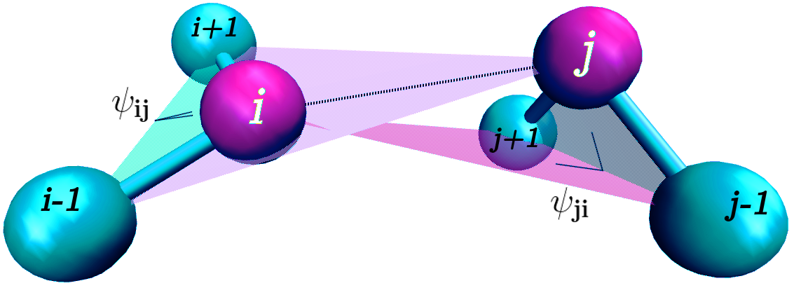
Figure 5: The idea of the PID angles. The interaction between residues $i$ and $j$ involves angles $\Psi_{ij}$ (defined by $i-1,i,i+1$ and $j$ beads) and $\Psi_{ji}$ (defined by $j-1,j,j+1$ and $i$ beads).

Those planes are shown in Fig. 5. The potential for each pair of residues is described by one distance $r_{i,j}$ and two pseudo-improper-dihedral (PID) angles $\Psi_{i,j}$ and $\Psi_{j,i}$. The potential is a product of three terms: $V(\psi_{i,j},\psi_{j,i},r_{i,j})=\lambda_{i,j}(\psi_{i,j})\lambda_{j,i}(\psi_{j,i})\phi(r_{i,j})$, where $\phi(r_{i,j})$ is a L-J potential. The PID angle distributions show clear peaks for the bb and ss cases. We used the Boltzmann inversion to discover that $\lambda(\psi)$ is indeed a Gaussian-like function [21]. Because the peaks are narrow, instead of a Gaussian function we implemented two functions that vanish away from the peak (i.e. they have a compact support). The first of them is a fragment of a cosine function (used if the variable lcospid is T), shifted to the peak value $\psi_{0}$ and rescaled by the $\alpha$ parameter that is inversely proportional to the width of the peak:

$$\lambda(\psi)=\begin{cases}0.5\cdot\cos{[\alpha(\psi-\psi_{0})]}+0.5&\text{when $-\pi<\alpha(\psi-\psi_{0})<\pi$}\\ 0&\text{otherwise}\end{cases}$$ (3)

The second equation gives a very similar shape of $\lambda(\psi)$, but is made from algebraic sigmoid functions, so it is faster (here $\upsilon=\alpha(\psi-\psi_{0})$):

$$0.5\cdot\cos{\upsilon}+0.5\approx\frac{(\upsilon/\pi)^{2}-2\cdot|\upsilon/\pi|+1}{2\cdot(\upsilon/\pi)^{2}-2\cdot|\upsilon/\pi|+1}$$ (4)

The distributions of the PID angles for the bb and ss cases are different so $V=V^{ss}+V^{bb}$. For the ss contacts, $V^{ss}(\psi_{A},\psi_{B},r)=\lambda^{ss}(\psi_{A})\lambda^{ss}(\psi_{B})\phi^{ss}(r)$. It turns out that the supports of $\lambda^{bb}$ and $\lambda^{ss}$ do not overlap. This makes the program faster (it computes only one $\lambda$ at a time).

The value of $r_{min}$ for the ss cases depends on which pair of amino acids is interacting. All values of $r_{min}$ are listed in the paramfile (in the same place as for the quasi-adiabatic potential).

The bb PID angle distribution has two peaks ($\psi_{0}^{bb+}$ and $\psi_{0}^{bb-}$), corresponding to the anti-parallel and parallel $\beta$ strands, so the bb potential has two corresponding terms:

$$\lambda_{bb}(\psi)=\begin{cases}0.5\cdot\cos{[\alpha^{bb+}(\psi-\psi_{0}^{bb+})]}+0.5&\text{when $-\pi<\alpha^{bb+}(\psi-\psi_{0}^{bb+})<\pi$}\\ 0.5\cdot\cos{[\alpha^{bb-}(\psi-\psi_{0}^{bb-})]}+0.5&\text{when $-\pi<\alpha^{bb-}(\psi-\psi_{0}^{bb-})<\pi$}\\ 0&\text{otherwise}\end{cases}$$ (5)

These two terms correspond to a left- and right- handed $\alpha$-helix in the case of $i,i+3$ interactions, so only one of them is used to mimic right-handedness of most of the $\alpha$-helices in proteins.

The repulsive part of the LJ potential should always be present for small distances, to prevent the residues from passing through one another (the excluded volume effect). So even if $\lambda$ is set to 0, the repulsive potential should not vanish. Therefore:

$$V^{bb}(\psi_{A},\psi_{B},r)=\begin{cases}\lambda^{bb}(\psi_{A})\lambda^{bb}(\psi_{B})\phi^{bb}(r)&\text{when $r>r_{min}^{bb}$}\\ \phi^{bb}(r)+(1-\lambda^{bb}(\psi_{A})\lambda^{bb}(\psi_{B}))\epsilon^{bb}&\text{otherwise}\end{cases}$$ (6)

For the bb case, $r_{min}$ is stored in the variables rbb1 and rbb2(corresponding to the ⁺ and ^- cases). The default values are $r_{min}^{+}=5.6$ Å  and $r_{min}^{-}=6.2$ Å. Other default parameters are: $\alpha^{bb+}=6.4$, $\alpha^{bb-}=6.0$, $\alpha^{ss}=1.2$, $\psi_{0}^{ss}=-0.23$ rad, $\psi_{0}^{bb+}=1.05$ rad, $\psi_{0}^{bb-}=-1.44$ rad. The fit to the statistical potential is available in ref. [21].

The depth of the L-J potential $\phi$ does not have to be uniform and always equal to 1 $\epsilon$. For bb contacts, $\epsilon^{bb}$ can be set in the variable epsbb. By default $\epsilon^{bb}=1$ $\epsilon$. If the variable lmj is set to T, the values of $\epsilon^{ss}$ for each possible pair of amino acids are taken from a Miyazawa-Jernigan matrix [24], which can be supplied by the paramfile. Otherwise $\epsilon^{ss}=1$ $\epsilon$. We include the paramfiles with the MDCG matrix derived from all-atom simulations [25] multiplied by 0.05 (parametersMD05.txt). The best agreement with the experiment for the PID model is accomplished for the MDCG matrix multiplied by a factor between 0 and 0.1 [21]. IDPs are strongly hydrated, which may be the cause of such small values. We include multiplier 0.05, because 0.1 turned out to lead to excessive aggregation of many chains (in ref. [21], the PID model is parameterized only for single chains). In example 2 (attached with the program) we use $\alpha$-synuclein, a strongly hydrated IDP that was extensively studied [26, 27]. The parameters used in example 2 should be a good starting point for recreating its properties (like the number of contacts), but further parameterization is probably needed.

Long sidechains have significant flexibility, resulting in broad distributions of C_α-C_α distances for ss contacts [13]. To recreate this we introduced a modified form of the L-J potential, shown below (it is turned on by the lsink variable, parameter $r_{min}^{bb}$ is specified by the variable cut, parameters $r_{min}^{ss}$ are different for each possible pair of amino acids and are taken from the paramfile):

$$\phi^{ss}(r)=\begin{cases}\epsilon^{ss}\left[{\left(\frac{r^{ss}_{min}}{r}\right)}^{12}-2\left(\frac{r^{ss}_{min}}{r}\right)^{6}\right]&\text{when $r>r_{min}^{ss}$}\\ -\epsilon^{ss}&\text{when $r_{min}^{ss}>r>r_{min}^{bb}$}\\ \epsilon^{ss}\left[{\left(\frac{r^{bb}_{min}}{r}\right)}^{12}-2\left(\frac{r^{bb}_{min}}{r}\right)^{6}\right]&\text{when $r_{min}^{bb}>r$}\end{cases}$$ (7)

4.2.3 Electrostatics

The electrostatic interactions for the quasi-adiabatic and pseudo-improper-dihedral potentials are the same (unless the variable lepid is set to T, which is an untested feature). They are described by the Debye-Hueckel (D-H) screened electrostatic potential $V_{D-H}(r_{i,j})=\frac{q_{i}q_{j}\exp{(-r_{i,j}/s)}}{4\pi\varepsilon\varepsilon_{0}r_{i,j}}$, where the screening length $s$ is defined in the variable screend and the charges $q_{i},q_{j}$ are 0, +1 or -1, based on the charge defined in the paramfile (in our units the elementary charge $e=1$).

The electric permittivity $\varepsilon$ is constant if the variable lecperm is T, but if lecperm is F, a distance-dependent $\varepsilon=4$ Å$/r_{i,j}$ is used [28]. In both cases $\varepsilon$ (or the coefficient before $r_{i,j}^{-1}$) is included in the amplitude of the D-H interactions, coul. Default values of this amplitude are 85 $\epsilon\cdot$Å$\cdot$Å  (for the distance-dependent $\varepsilon=4$ Å$/r_{i,j}$) and 2.63 $\epsilon\cdot$Å  (for the constant $\varepsilon=80$ case).

The electrostatic interactions between the oppositely-charged residues can be treated differently by setting the variable lrepcoul T. Then the attractive interactions between those residues are governed by the custom potential (quasi-adiabatic or pseudo-improper-dihedral). The repulsive interactions between same-charged residues are still treated by the D-H potential.

4.3 Disulfide bonds

For structured proteins, cysteines are treated as every other amino acid, with the exception of those specified in the SSBOND records in the PDB file - those are connected harmonically with the spring constant H1 and the equilibrium distance 6 Å. If the variable lsslj is T, even the cysteines in the SSBOND records are treated as other amino acids.

The options for the disordered case (when lcpot is T) work only for the quasi-adiabatic version of the model. The default option is the same harmonic potential as above, but it is quasi-adiabatically turned on when the criteria of an ss contact formation are fulfilled, together with two additional conditions: cysteines are not part of any other disulfide bond, and the sum of the numbers of their neighbours must be smaller than neimaxdisul (9 by default). The number of neighbours is computed as the number of residues within a radius rnei (default 7.5 Å) from a given cysteine. This harmonic potential can be quasi-adiabatically turned off if $(r_{ij}-6\text{ \AA})^{2}>0.1$ Ų and the total number of neighbours is smaller than neimaxdisul. Thus, the disulfide bond formation in disordered proteins can be turned off by specifying neimaxdisul$=-1$. Those neighbour calculations are supposed to mimic the effect of solvent accessibility, which is crucial for the disulfide bond oxidation and reduction [29].

If the variable lsselj is T, a special L-J potential with the depth dislj (4 $\epsilon$ by default) is used. When this special type of contact is quas-adiabatically turned on between a pair of cysteines, they can no longer make such pairs with other cysteines. This contact obeys the same criteria for formation and breaking as any other ss contact.

5 Simulation protocols, geometries and boundary conditions

All the variables that describe time in the sections below are given in $\tau$ units. Every type of simulation can be repeated multiple times with different random seed during one execution of the program. Each repeat is called a trajectory. The variable ntraj determines the number of repeats. Out of all residues, the first nen1 of them can be ,,frozen” - they will not move during the simulation (which may greatly reduce computation time).

5.1 Simulation protocols

5.1.1 Equilibrium simulations

With the default options the proteins are put in an infinite space and there are no external forces acting upon them (except for friction and the thermostat). Time of the whole simulation is mstep. All the other protocols are preceded by the equilibration period. Boundary conditions may then be different, but the duration of the equilibration is always specified by the variable kteql. However the simulation time never exceeds mstep.

5.1.2 Stretching by the tips of the AFM

If the lvelo variable is T, the first and last residues are caught by harmonic springs with the spring constant HH1 and pulled apart in the direction determined by the vector connecting both residues. To perform stretching simulations with spring constant resembling real AFM tips, please set HH1 to 0.06 $\epsilon/$Ų in the inputfile [6].

The springs start to act after the equilibration and this vector is also determined at the time $t=$kteql. Then, the springs are moved apart from each other along this vector with the velocity velo (in Å/$\tau$ units). The variable lforce has a similar effect, but the pulling occurs with a constant force (specified in the variable coef, in $\epsilon/$Å  units) acting on the terminal residues, instead of the constant speed.

5.1.3 Folding simulations

When the variables lconftm or lmedian are T, the simulation starts from a straight line or a self-avoiding random walk (which is controlled by the variable lsawconftm). Then, for lconftm, the average time of contact formation is computed for each native contact. The average is taken over all trajectories.

For lmedian, the program computes the median folding time. The folding time is defined as the time where all the native contacts are established [12, 30]. If more than half of the trajectories did not end in the folded state, the simulation ends (because then it is impossible to compute the median folding time). Trajectories during folding simulations may end after mstep timesteps, or after the native conformation is reached (if the variable lnatend is set to T).

5.1.4 Unfolding simulations

When the variable lunfold is T, the simulation starts from the native structure and the average time of contact breaking is computed for each native contact. The average is taken over all trajectories. Those simulations are usually performed in the temperature temp higher than the room temperature. If the variable lthermo is T, thermodynamic properties such as the heat capacity $C_{V}=\frac{<E^{2}>-<E>^{2}}{T^{2}}$ are computed. A set of different temperatures can be simulated by specifying different tstart and tend.

5.1.5 Deformations of the simulation box

When the variable lwall is T, the simulation does not occur in infinite space but in a box. Currently all the simulation protocols supported in this case require a specified density (in residue/ų units), so the variable ldens must be set to T. In the case of proteins from a PDB file, the box sizes in the CRYST1 record are initially used. For disordered proteins, the initial density is sdens and the simulation box is a cube. The chains (straight lines or self-avoiding walks, as set in lsawconftm) are constructed randomly in the box. If a chain goes beyond the box, the box size is increased to fit it (unless there are periodic boundary conditions in the initial state, which is controlled by the lcpb variable). It means that the actual density during the start of the dynamics may be even lower than sdens. Then, the box shrinks uniformly in all the 3 dimensions (the wall speed is densvelo) until it reaches the target density tdens. Then the box size does not change for a time equal to ktrest.

If the variable loscillate is T, the box starts to deform again (after the resting period specified in ktrest). There are two possible modes of oscillating the box walls: pulling and shearing (determined by the lshear variable). In the pulling mode, the distance between the two walls perpendicular to the Z axis changes periodically. In the shearing mode, the same two walls move periodically along the X axis.

The oscillation starts by achieving the maximal amplitude of oscillation. If the variable lampstrict is T, the amplitude ampstrict is the wall displacement (in the Z direction for pulling, in the X direction for shearing) in Å. Otherwise, the amplitude amp is determined relative to the initial distance between the two moving walls. After the walls are moved to their maximum displacement, there is another resting period (with a duration time ktrest) for equilibration. Then the displacement $s$ changes periodically: $s(t)=s_{0}(1-A\cos{2\pi(t/period)})$, where the period of the oscillations is the variable period and the amplitude $A$ is either amp$\cdot s_{0}$ or ampstrict. The number of full oscillations is specified by kbperiod. If the variable lconstvol is T, the wall distance in the X and Y directions is also changed to maintain the constant volume of the box. After oscillations (or after equilibration if loscillate is F), the system is equilibrated again (with the resting time ktrest) and then the walls in the Z direction extend to $2s_{0}$ (if the variable lpullfin is T, otherwise the box does not deform anymore).

5.2 Boundary conditions

As mentioned before, by default the proteins are in an infinite space. Setting lwall T makes the simulation box finite. Then, by default the two walls perpendicular to the Z axis are ,,solid”. Setting lpbc T results in periodic boundary conditions only in the X and Y dimensions. To make them in all the three dimensions, the variable lnowal must be also set to T.

The variable lwalls is used to get ,,solid” walls in the X and Y directions. Here ,,solid” means repulsive, as decribed by the potential $V_{wall}=\frac{-\epsilon}{9d^{9}}$, where $d$ is the distance from a residue to the wall [31].

The walls in the $Z$ direction may have different ways of interacting with the residues. However, initially they always interact via $V_{wall}$ and there is a specific time when other special types of interaction may be turned on for the two walls along the Z axis. This specific time is controlled by the variable kconnecttime. Here are its possible values:

kconnecttime	description
1	just after reaching target density tdens
3	after waiting for ktrest after reaching tdens
5	just after reaching the maximal amplitude of oscillations
7	just after oscillations
9	never

Table 2: Meaning of the kconnecttime variable

Below are listed all the tested ways to introduce interactions between the residues and the two walls that perpendicular to the $Z$ direction.

5.2.1 FCC walls

If the variable lfcc is T, each of the walls is made from two layers of beads arranged in a face-centered-cubic lattice cut through the [111] crystallographic direction. The lattice constant is af. The beads are immovable (except for the movement of the whole wall) and interact via the L-J potential with the same amplitude as for disulfide bonds, dislj, and the same minimum, walmindist. The interactions are quasi-adiabatically turned on when the residue comes closer than walmindist (the minimum of the L-J potential) to one of the beads and is broken in the same way when the distance $r_{i,\text{bead}}>\texttt{cntfct}\cdot 2^{-1/6}\cdot\text{{walmindist}}$.

5.2.2 Flat attractive walls

If ljwal is T, the residues interact with the wall via the same quasi-adiabatic L-J potential as above. The only difference is that when the residue comes closer than walmindist to the wall, it starts to be attracted by an artificial bead with the same X and Y coordinates as the residue’s coordinates when it crosses the walmindist distance. This artificial bead does not attract other residues and disappears when $r_{i,\text{bead}}>\texttt{cntfct}\cdot 2^{-1/6}\cdot\text{{walmindist}}$. This can give a significant computational speed-up, as those artificial beads are not checked when updating the Verlet list.

If the variables ljwal and lfcc are F, all the residues closer than walmindist to the wall are harmonically attached to it, with the spring constant HH1 and the equilibrium distance equal to the distance in the moment of turning on the interaction. The default value of HH1 is 30 $\epsilon/$Ų, which corresponds to strong, covalent bonding.

6 Advantages and disadvantages of the program

The quasi-adiabatic and pseudo-improper-dihedral potentials are specifically designed for simulating intrinsically disordered proteins. The first potential generalizes the idea of the contact interactions taken from the structure-based Go model [6] (which is also included in the program). This enables the simulation of partially disordered proteins, like the structured domains connected by flexible linkers (e.g. cellulosome proteins [32]), proteins with disordered tracts (e.g. huntingtin [33]) and large protein complexes with different amounts of complexity (e.g. gluten [34]). Our program was used to simulate the last case, gluten, which (according to our knowledge) was never simulated before [35]. The program was also used to study aggregation of polyglutamine, which is a fully disordered protein [36]. These two applications (both involving simulations of thousands of residues for more than a milisecond) prove the suitability of the quasi-adiabatic potential for large protein systems. One disadvantage of the program is that (in the present form) it is not yet prepared to study folding-upon-binding mechanisms [37].

The main strength of the program is allowing the study of large protein systems (in relatively long timescales), while retaining their protein nature. For the largest systems (like gluten) the faster quasi-adiabatic potential is best-suited [13]. Smaller systems can be studied with better accuracy by the slower pseudo-improper-dihedral potential [21]. The program may be also used to study fully structured proteins [1, 3, 6, 8, 9, 10, 12, 38, 39, 40]

There are many other packages that may be used for implicit solvent, coarse-grained protein molecular dynamics [41, 42, 43, 44, 45, 46, 47, 48], but none of them implements the quasi-adiabatic and pseudo-improper-dihedral potentials presented here. Many of them allow user-defined force fields [41, 42, 44, 46, 48] and/or are open-source [43, 44, 45], however, none of them allows for an easy addition of dynamic contacts, switched on and off based on criteria of distance, direction and coordination number (see section 4.2.1). We discuss the advantages of using those criteria in a one-bead-per-residue model elsewhere [13]. The novel pseudo-improper-dihedral potential (described in section 4.2.2 and in [21]) also cannot be easily added to the existing packages (with the possible exception of [44] and [45]). The main disadvantage of using our software is that in the current state it is not as scalable as the alternatives (it cannot be effectively run on GPUs and it does not support MPI, only openMP).

References

- [1] M. Sikora, J. I. Sułkowska and M. Cieplak, Mechanical strength of 17 134 model proteins and cysteine slipknots, PLoS Comput. Biol. 5 (2009) e1000547.
- [2] J. I. Sułkowska and M. Cieplak, Selection of optimal variants of go-like models of proteins through studies of stretching, Biophys. J. 95, (2008) 317491.
- [3] K. Wołek, Á. Gómez-Sicilia and M. Cieplak, Determination of contact maps in proteins: a combination of structural and chemical approaches, J. Chem. Phys. 143, (2015) 243105.
- [4] Y. Zhao, M. Chwastyk, and M. Cieplak, Topological transformations in proteins: effects of heating and proximity of an interface, Sci. Rep. 7, (2017) 39851.
- [5] Ł. Mioduszewski and M. Cieplak, Disordered peptide chains in an -c-based coarse-grained model, Phys. Chem. Chem. Phys. 20, (2018) 19057-19070.
- [6] Ł. Mioduszewski and M. Cieplak, Viscoelastic properties of wheat gluten in a molecular dynamics study, PLOS Comput. Biol. 17(3), (2021) e1008840.
- [7] Ł. Mioduszewski, B. Różycki and M. Cieplak, Pseudo-improper-dihedral model for intrinsically disordered proteins, J. Chem. Theory Comput. 16(7), (2020) 4726–4733.
- [8] Y. Zhao, M. Chwastyk, and M. Cieplak, Structural entanglements in protein complexes, J. Chem. Phys. 146, (2017) 225102.
- [9] M.Chwastyk, A. Galera–Prat, M. Sikora, À. Gómez-Sicilia, M. Carrión-Vázquez, and M. Cieplak, Theoretical tests of the mechanical protection strategy in protein nanomechanics, Proteins 82, (2014) 717-726.

References

- [1] M. Cieplak and T.X. Hoang, Universality classes in folding times of proteins. Biophys J. 84(1) (2003) 475-488.
- [2] T. Veitshans, D. Klimov and D. Thirumalai, Protein folding kinetics: time scales, pathways and energy landscapes in terms of sequence-dependent properties, Folding Des. 2 (1997) 1-22.
- [3] P. Szymczak and M. Cieplak, Stretching of proteins in a uniform flow. J. Chem. Phys. 125(16) (2006) 164903.
- [4] M. P. Allen and D. J. Tildesley, Computer Simulation of Liquids, Oxford University Press, New York, 1987.
- [5] J. M. Haile, A Primer on the Computer Simulation od Atomic Fluids by Molecular Dynamics Clemson University, Clemson, NC (1980).
- [6] M. Sikora, J. I. Sułkowska and M. Cieplak, Mechanical strength of 17 134 model proteins and cysteine slipknots. PLoS Comp. Biol. 5 (2009) e1000547.
- [7] A. B. Poma, M. Chwastyk and M. Cieplak, Polysaccharide-protein complexes in a coarse-grained model. J. Phys. Chem. B. 119 (2015) 12028-12041.
- [8] M. Cieplak and M. O. Robbins, Nanoindentation of virus capsids in a molecular model. J. Chem. Phys. 132 (2010) 015101.
- [9] K. Wołek and M. Cieplak, Self-assembly of model proteins into virus capsids. J. Phys. Cond. Matter 47 (2017) 474003.
- [10] T. X. Hoang and M. Cieplak, Molecular dynamics of folding of secondary structures in Go-like models of proteins, J. Chem. Phys. 112 (2000) 6851-6862.
- [11] L. M. Pietrek, L.S. Stelzl and G. Hummer, Hierarchical ensembles of intrinsically disordered proteins at atomic resolution in molecular dynamics simulations, J. Chem. Theory Comput. 16(1) (2020) 725-737.
- [12] K. Wołek and M. Cieplak, Criteria for folding in structure-based models of proteins. J. Chem. Phys. 144 (2016) 185102.
- [13] Ł. Mioduszewski and M. Cieplak, Disordered peptide chains in an -c-based coarse-grained model. Phys. Chem. Chem. Phys. 20 (2018) 19057-19070.
- [14] A. Ghavami, E. V. D. Giessen and P. R. Onck, Coarse-grained potentials for local interactions in unfolded proteins. J. Chem. Theory Comput. 9 (2013) 432–440.
- [15] B. Schuler, E. A. Lipman, P. J. Steinbach, M. Kumke, and W. A. Eaton, Polyproline and the ,,spectroscopic ruler” revisited with single-molecule fluorescence. Proc. Natl. Acad. Sci. USA 102 (2005) 2754–2759.
- [16] G. Settanni, T. X. Hoang, C. Micheletti and A. Maritan (2002) Folding pathways of prion and doppel. Biophys. J. 83 (2002) 3533-3541.
- [17] J. Tsai, R. Taylor, C. Chothia and M. Gerstein, The packing density in proteins: Standard radii and volumes. J. Mol. Biol. 290 (1999) 253-266.
- [18] J. I. Sułkowska and M. Cieplak, Mechanical stretching of proteins – A theoretical survey of the Protein Data Bank, topical review, J. Phys.: Cond. Mat. 19 (2007) 283201.
- [19] K. Wołek, Á. Gómez-Sicilia and M. Cieplak, Determination of contact maps in proteins: a combination of structural and chemical approaches, J. Chem. Phys. 143 (2015) 243105.
- [20] A. Kolinski, Protein modeling and structure prediction with a reduced representation. Acta Biochim. Pol. 51 (2004) 349-371.
- [21] Ł. Mioduszewski, B. Różycki and M. Cieplak, Pseudo-improper-dihedral model for intrinsically disordered proteins, J. Chem. Theory Comput. 16(7) (2020) 4726–4733.
- [22] M. Enciso and A. Rey, A refined hydrogen bond potential for flexible protein models. J. Chem. Phys. 132 (2010) 235102.
- [23] N. B. Hung, D.-M. Le and T. X. Hoang, Sequence dependent aggregation of peptides and fibril formation. J. Chem. Phys. 147 (2017) 105102.
- [24] S. Miyazawa and R. L. Jernigan, Residue – Residue Potentials with a Favorable Contact Pair Term and an Unfavorable High Packing Density Term, for Simulation and Threading, J. Mol. Biol. 256 (1996) 623-644.
- [25] M. R. Betancourt and S. J. Omovie, Pairwise energies for polypeptide coarse-grained models derived from atomic force fields, J. Chem. Phys. 130 (2009) 195103.
- [26] P. Robustelli, S. Piana and D. E. Shaw, Developing a molecular dynamics force field for both folded and disordered protein states, Proc. Natl. Acad. Sci. USA 115(21) (2018) 4758-4766.
- [27] M. Chwastyk, M. Cieplak, Conformational Biases of -Synuclein and Formation of Transient Knots. J. Phys. Chem. B. 124(1) (2020) 11-19.
- [28] V. Tozzini, J. Trylska, C.E. Chang and J.A. McCammon, Flap opening dynamics in hiv-1 protease explored with a coarse-grained model, J. Struct. Biol. 157 (2007) 606-615.
- [29] M. Qin, W. Wang and D. Thirumalai, Protein Folding Guides Disulfide Bond Formation. Proc. Natl. Acad. Sci. USA 112 (2015) 11241-11246.
- [30] Y. Zhao, M. Chwastyk, and M. Cieplak, Topological transformations in proteins: effects of heating and proximity of an interface, Sci. Rep. 7, (2017) 39851.
- [31] M. Cieplak and M. O. Robbins, Nanoindentation of 35 virus capsids in a molecular model: Relating mechanical properties to structure, PLoS ONE 8 (2013) e63640.
- [32] B. Różycki, P.-A. Cazade, S. O’Mahony, D. Thompson, M. Cieplak, The length but not the sequence of peptide linker modules exerts the primary influence on the conformations of protein domains in cellulosome multi-enzyme complexes. Phys. Chem. Chem. Phys. 19 (2017) 21414-21425.
- [33] F. Giorgini, Polyglutamine provides huntingtin flexibility, Proc. Natl. Acad. Sci. USA 110(36) (2013) 14516-14517.
- [34] H. Wieser. Chemistry of gluten proteins. Food Microbiol. 24(2) (2007) 115–119.
- [35] Ł. Mioduszewski and M. Cieplak, Viscoelastic properties of wheat gluten in a molecular dynamics study, PLOS Comput. Biol. 17(3) (2021) e1008840.
- [36] Ł. Mioduszewski and M. Cieplak, Protein droplets in systems of disordered homopeptides and the amyloid glass phase, Phys. Chem. Chem. Phys. 22 (2020) 15592–15599.
- [37] P. Robustelli, S. Piana and D. E. Shaw, Mechanism of Coupled Folding-upon-Binding of an Intrinsically Disordered Protein, J. Am. Chem. Soc. 142(25) (2020) 11092–11101.
- [38] Y. Zhao, M. Chwastyk, and M. Cieplak, Structural entanglements in protein complexes, J. Chem. Phys. 146, (2017) 225102.
- [39] M.Chwastyk, A. Galera–Prat, M. Sikora, À. Gómez-Sicilia, M. Carrión-Vázquez, and M. Cieplak, Theoretical tests of the mechanical protection strategy in protein nanomechanics, Proteins 82, (2014) 717-726.
- [40] M. Chwastyk, A. M. Vera, A. Galera-Prat, M. Gunnoo, D. Thompson, M. Carrión-Vázquez, and M. Cieplak, Non-local effects of point mutations on the stability of a protein module, J. Chem. Phys. 147, (2017) 105101.
- [41] M. J. Abraham, T. Murtola, R. Schulz, S. Páll, J. C. Smith, B. Hess and E. Lindahl, GROMACS: High performance molecular simulations through multi-level parallelism from laptops to supercomputers, SoftwareX, 1–2 (2015) 19-25.
- [42] S. Plimpton, Fast Parallel Algorithms for Short-Range Molecular Dynamics, J. Comp. Phys. 117 (1995) 1-19.
- [43] A. Liwo, S. Oldziej, C. Czaplewski, D. S. Kleinerman, P. Blood and H. A. Scheraga, Implementation of molecular dynamics and its extensions with the coarse-grained UNRES force field on massively parallel systems; towards millisecond-scale simulations of protein structure, dynamics, and thermodynamics, J. Chem. Theory Comput. 6 (2010) 890-909.
- [44] P. Eastman, J. Swails, J. D. Chodera, R. T. McGibbon, Y. Zhao, K. A. Beauchamp, L.-P. Wang, A. C. Simmonett, M. P. Harrigan, C. D. Stern, R. P. Wiewiora, B. R. Brooks, V. S. Pande, OpenMM 7: Rapid Development of High Performance Algorithms for Molecular Dynamics, PLoS Comput. Biol. 13 (2017) e1005659.
- [45] H. Kenzaki, N. Koga, N. Hori, R. Kanada, W. F. Li, K. Okazaki, X. Q. Yao and S. Takada, CafeMol: A Coarse-Grained Biomolecular Simulator for Simulating Proteins at Work, J. Chem. Theory Comput. 7(6) (2011) 1979-1989.
- [46] J. A. Anderson, J. Glaser, and S. C. Glotzer, HOOMD-blue: A Python package for high-performance molecular dynamics and hard particle Monte Carlo simulations, Comput. Mater. Sci. 173 (2020) 109363.
- [47] I. A. Solov’yov, A. V. Yakubovich, P. V. Nikolaev, I. Volkovets, and A. V. Solov’yov, Meso Bio Nano Explorer - a universal program for multiscale computer simulations of complex molecular structure and dynamics, J. Comput. Chem. 33 (2012) 2412-2439.
- [48] K. J. Bowers, E. Chow, H. Xu, R. O. Dror, M. P. Eastwood, B. A. Gregersen, J. L. Klepeis, I. Kolossvary, M. A. Moraes, F. D. Sacerdoti, J. K. Salmon, Y. Shan and D. E. Shaw, Scalable Algorithms for Molecular Dynamics Simulations on Commodity Clusters, Proc. ACM/IEEE Conf. Supercomput. SC06 (2006).