A Moving Mesh Finite Element Method for Bernoulli Free Boundary Problems

Abstract

A moving mesh finite element method is studied for the numerical solution of Bernoulli free boundary problems. The method is based on the pseudo-transient continuation with which a moving boundary problem is constructed and its steady-state solution is taken as the solution of the underlying Bernoulli free boundary problem. The moving boundary problem is solved in a split manner at each time step: the moving boundary is updated with the Euler scheme, the interior mesh points are moved using a moving mesh method, and the corresponding initial-boundary value problem is solved using the linear finite element method. The method can take full advantages of both the pseudo-transient continuation and the moving mesh method. Particularly, it is able to move the mesh, free of tangling, to fit the varying domain for a variety of geometries no matter if they are convex or concave. Moreover, it is convergent towards steady state for a broad class of free boundary problems and initial guesses of the free boundary. Numerical examples for Bernoulli free boundary problems with constant and non-constant Bernoulli conditions and for nonlinear free boundary problems are presented to demonstrate the accuracy and robustness of the method and its ability to deal with various geometries and nonlinearities.

AMS 2020 Mathematics Subject Classification. 65M60, 65M50, 35R35, 35R37

Key Words. free boundary problem, moving boundary problem, moving mesh, finite element, pseudo-transient continuation.

1 Introduction

Bernoulli free boundary problems (FBPs) arise in ideal fluid dynamics, optimal insulation, and electro chemistry [17] and serve as a prototype of stationary FBPs. They have been extensively studied theoretically and numerically; e.g., see [2, 7, 9, 10, 12, 15, 17, 36, 42]. To be specific, we consider here a typical Bernoulli FBP

$$\begin{cases}-\Delta u=0,&\text{ in }\Omega\\ u=1,&\text{ on }\Gamma_{1}\\ u=0,&\text{ on }\Gamma_{2}\\ -\frac{\partial u}{\partial n}=\lambda,&\text{ on }\Gamma_{2}\end{cases}$$ (1)

where $\Omega$ is a connected domain in $\mathbb{R}^{2}$ (see Fig. 1), $\lambda$ is a positive constant, $\Gamma_{1}\cup\Gamma_{2}=\partial\Omega$, $\Gamma_{1}$ is given and fixed, and $\Gamma_{2}$ is unknown a priori and part of the solution. We emphasize that the numerical method studied in this work can be applied to more general FBPs without major modifications, and several such examples are presented in Section 5.

The Neumann boundary condition in (1) is called the Bernoulli condition. This condition can be shown to be equivalent to $|\nabla u|=\lambda$ (with the help of the Dirichlet boundary condition on $\Gamma_{2}$). Moreover, the problem is called an exterior (or interior) Bernoulli problem when $\Gamma_{2}$ is exterior (or interior) to $\Gamma_{1}$ (cf. Fig. 1). It is known [2, 5, 17] that an exterior Bernoulli problem has a solution for any $\lambda>0$ and such a solution is unique and elliptic when the domain enclosed by $\Gamma_{1}$ is convex. Loosely speaking, a solution is said to be elliptic (or hyperbolic) if $\Gamma_{2}$ is getting closer to (or moving away from) $\Gamma_{1}$ as $\lambda$ increases. On the other hand, an interior Bernoulli problem has a solution only for $\lambda$ large enough and such solutions are not unique in general. Both elliptic and hyperbolic solutions can co-exist for the same value of $\lambda$ for interior problems.

While the differential equation and boundary conditions are linear, the problem (1) is actually highly nonlinear due to the coupling between $u$ and $\Omega$. A number of numerical methods have been developed for solving Bernoulli FBPs; e.g., see a summary of early works for general FBPs [12, Chapter 8], the explicit and implicit Neumann methods [17], a combined level set and boundary element method [31], shape-optimization-based methods [14, 15, 21, 36], the cut finite element method [9], the quasi-Monte Carlo method [7], the comoving mesh method [40], and the singular boundary method [11]. A common theme among those methods is trial free boundary and thus iterating between the update of the free boundary and the solution of the corresponding boundary value problem. Challenges for this approach include how to choose the initial guess for $\Gamma_{2}$ to make the iteration convergent and to re-generate or deform the mesh to fit the varying domain.

(a) Exterior problem

(b) Interior problem

Figure 1: Illustration of the domain for exterior and interior Bernoulli FBPs.

In this work we shall present a moving mesh finite element method for the numerical solution of Bernoulli FBPs. The method is based on the pseudo-transient continuation (e.g., see Fletcher [16, Section 6.4]) with which we construct an equivalent time-dependent problem (a moving boundary problem or an MBP), march it until the steady state is reached, and take the steady-state solution as the solution of Bernoulli FBP (1). The pseudo-transient continuation is widely used for difficult nonlinear problems in science and engineering because it can be made convergent for a large class of initial solutions. Another advantage of using the pseudo-transient continuation is that the corresponding MBP can be solved readily with boundary-fitted meshes using the finite element method and the Moving Mesh PDE (MMPDE) method. The MMPDE method has been developed for general mesh adaptation and movement; e.g., see [28, 29]. It moves the mesh points continuously in time while providing an effective control of mesh quality and concentration. Most importantly, the method guarantees that the mesh is free of tangling for any domain (convex or concave) in any spatial dimension [27]. This mesh nonsingularity is crucial for any mesh-based computation including that for FBPs. On the other hand, close attention shluld be paid to the update of the free boundary where both the gradient of the finite element solution and the normal to the approximate boundary are needed in the computation of the Bernoulli condition but not defined at boundary vertices in the standard finite element approximation on a simplicial mesh. Their re-constructions are required and such re-constructions can affect the spatial accuracy of the overall computation. Two re-construction approaches, (area-)averaging and quadratic least squares fitting, will be discussed.

An outline of this paper is as follows. The pseudo-transient continuation and the corresponding MBP will be described in Section 2. Section 3 is devoted to the description of the moving mesh FEM. Numerical examples for Bernoulli FBPs and nonlinear FBPs are presented in Sections 4 and 5, respectively. Finally, conclusions and further comments are given in Section 6.

2 The pseudo-transient continuation

For Bernoulli FBP (1), we consider the time-dependent problem

$$\begin{cases}\frac{\partial u}{\partial t}-\Delta u=0,&\text{ in }\Omega,\text{ for }t>0\\ u=1,&\text{ on }\Gamma_{1}\\ u=0,&\text{ on }\Gamma_{2}\\ \dot{\Gamma}=-\frac{\partial u}{\partial n}-\lambda,&\text{ on }\Gamma_{2}.\end{cases}$$ (2)

This system is marched until the steady state is reached and the obtained steady-state solution is taken as the solution of Bernoulli FBP (1).

Immediate questions are if MBP (2) has a steady-state solution and whether or not such a solution is stable. They are related to the asymptotic behavior of solutions of MBPs and the stability of their steady-state solutions, an area of active research; e.g., see [13, 18, 44, 46]. Unfortunately, none of the available theoretical results seems applicable to (2). Nevertheless, we can gain some insight from a formal analysis. We take the exterior problem as an example (cf. Fig. 2). From the maximum principle, we know that $u\geq 0$ on $\Omega$ and $\frac{\partial u}{\partial n}|_{\Gamma_{2}}\leq 0$. Consider a point $x$ on $\Gamma_{2}$. If $-\frac{\partial u}{\partial n}-\lambda>0$ at this point, then $\dot{\Gamma}>0$ and $x$ moves outward and farther away from $\Gamma_{1}$. Recall that $u|_{\Gamma_{1}}=1$ and $u|_{\Gamma_{2}}=0$. Thus, as the distance between $\Gamma_{1}$ and $\Gamma_{2}$ increases, $-\frac{\partial u}{\partial n}$ (and therefore, $\dot{\Gamma}=-\frac{\partial u}{\partial n}-\lambda$) will decrease, which means that the movement of $x$ will slow down. This continues until $-\frac{\partial u}{\partial n}-\lambda$ reaches zero. On the other hand, if $-\frac{\partial u}{\partial n}-\lambda<0$, $x$ will move inward and closer to $\Gamma_{1}$, which will cause $-\frac{\partial u}{\partial n}$ to increase and the movement of the boundary point to slow down until $-\frac{\partial u}{\partial n}-\lambda$ reaches zero. Thus, for either case $\Gamma_{2}(t)$ will reach a steady state and so does the domain $\Omega$. Once $\Omega$ gets close to its steady state, (2) behaves like a parabolic problem with a fixed domain and its solution will reach steady state too. Thus, (2) reduces to (1).

Figure 2: Illustration of boundary movement for MBP (2).

It is interesting to point out that the use of (2) can also be justified by shape optimization theory. Indeed, Bernoulli FBPs can be formulated as shape optimization problems; e.g., see [14, 15, 22]. One of the equivalent shape optimization problems for (1) is to minimize the cost function

$$J(\Omega)=\int_{\Omega}(|\nabla u|^{2}+\lambda^{2})d\mbox{\boldmath$x$}$$ (3)

subject to the PDE constraint

$$\begin{cases}-\Delta u=0,&\text{ in }\Omega\\ u=1,&\text{ on }\Gamma_{1}\\ u=0,&\text{ on }\Gamma_{2}.\end{cases}$$ (4)

Using shape optimization calculus [22, 38], we can find the variation of $J(\Omega)$ along a given vector field $V$ as

$$\delta J(\Omega)[\mbox{\boldmath$V$}]=\int_{\Gamma_{2}}\left(\lambda^{2}-(\frac{\partial u}{\partial n})^{2}\right)\mbox{\boldmath$V$}\cdot\mbox{\boldmath$n$}\;ds.$$ (5)

Thus, a descent direction for $J(\Omega)$ is to update $\Gamma_{2}$ along

$$-\left(\lambda^{2}-(\frac{\partial u}{\partial n})^{2}\right)\mbox{\boldmath$n$}=-(\lambda+\frac{\partial u}{\partial n})(\lambda-\frac{\partial u}{\partial n})\mbox{\boldmath$n$}.$$

The maximum principle implies that the solution to (4) is positive in $\Omega$ and $\frac{\partial u}{\partial n}\leq 0$ on $\Gamma_{2}$. Since $\lambda$ is positive, we have $(\lambda-\frac{\partial u}{\partial n})>0$ and the descent direction is proportional to $-(\lambda+\frac{\partial u}{\partial n})\mbox{\boldmath$n$}$. This suggests that $\Gamma_{2}$ can be updated along $-(\lambda+\frac{\partial u}{\partial n})\mbox{\boldmath$n$}$, i.e.,

$$\dot{\Gamma}=-\frac{\partial u}{\partial n}-\lambda\quad\text{ on }\Gamma_{2}.$$ (6)

This gives the boundary velocity in (2). Interestingly, trial free boundary methods (e.g., see [12, Chapter 8]) can be interpreted as a time discretization of the above equation. Moreover, Sunayama et al. [40] use

$$\begin{cases}-\Delta u=0,&\text{ in }\Omega\\ u=1,&\text{ on }\Gamma_{1}\\ u=0,&\text{ on }\Gamma_{2}\\ \dot{\Gamma}=-\frac{\partial u}{\partial n}-\lambda,&\text{ on }\Gamma_{2}.\end{cases}$$ (7)

The difference between this system and (2) is that the heat equation, instead of the Laplace equation, is used in (2). With (2), we can take full advantages of the pseudo-transient continuation in the numerical solution. Particularly, we can use automatic time stepsize selection procedures and extend the developed numerical method to more general FBPs (including nonlinear FBPs) without major modifications (cf. Section 5).

3 A moving mesh finite element solution for MBPs

In this section, we describe a moving mesh finite element method for solving MBP (2). The method solves (2) in a splitting manner at each time step: updates the boundary using the Euler scheme, moves the interior mesh points using the MMPDE moving mesh method, and integrates the underlying initial-boundary value problem using a Runge-Kutta scheme and linear finite elements. The method has been used in [33] for solving the porous medium equation. The method can be used for general MBPs although it is described here only for (2).

Algorithm 1 Moving mesh FEM for (2)

• Assume that $\mathcal{T}_{h}^{n}$ and $u_{h}^{n}$ at $t=t_{n}$ are known.

• Boundary update. Update the mesh vertices on $\Gamma_{2}$ using the Euler scheme,

  $$\mbox{\boldmath$x$}_{i}^{n+1}=\mbox{\boldmath$x$}_{i}^{n}+\Delta t_{n}\left.\left(-\nabla u_{h}^{n}\cdot\mbox{\boldmath$n$}-\lambda\right)\mbox{\boldmath$n$}\right|_{\mbox{\boldmath$x$}_{i}^{n}},\quad\forall\mbox{\boldmath$x$}_{i}^{n}\in\Gamma_{2}^{n}.$$ (8)

  Denote by $\Gamma_{2}^{n+1}$ the updated boundary and by $\tilde{\mathcal{T}}_{h}^{n+1}$ the mesh with the updated boundary. Thus, the vertices of $\tilde{\mathcal{T}}_{h}^{n+1}$ consist of the boundary vertices on $\Gamma_{2}^{n+1}$ and $\Gamma_{1}$ and the interior vertices of $\mathcal{T}_{h}^{n}$. Notice that the Euler update (8) generally will not result in an even distribution of the boundary vertices along the boundary. They can be made more evenly distributed in the next step (the mesh movement step) by allowing the boundary vertices to slide along the boundary.

• Movement of interior mesh vertices. Generate the new mesh $\mathcal{T}_{h}^{n+1}$ for $\Omega^{n+1}$ by moving the vertices of $\tilde{\mathcal{T}}_{h}^{n+1}$ using the MMPDE moving mesh method. The detail is given in Subsection 3.3.

• Solution of the initial-boundary value problem. Solve the IBVP

  $$\begin{cases}\frac{\partial u}{\partial t}-\Delta u=0,&\text{ in }\Omega(t)\\ u=1,&\text{ on }\Gamma_{1}\\ u=0,&\text{ on }\Gamma_{2}(t)\end{cases}$$ (9)

  on the moving mesh $\mathcal{T}_{h}(t)$ defined as the linear interpolation between $\mathcal{T}_{h}^{n}$ and $\mathcal{T}_{h}^{n+1}$, i.e.,

  $$\mbox{\boldmath$x$}_{i}(t)=\frac{t_{n+1}-t}{\Delta t_{n}}\mbox{\boldmath$x$}_{i}^{n}+\frac{t-t_{n}}{\Delta t_{n}}\mbox{\boldmath$x$}_{i}^{n+1},\quad i=1,...,N_{v},\quad t\in[t_{n},t_{n+1}].$$ (10)

  In this step, the domain moves from $\Omega^{n}$ to $\Omega^{n+1}$ and is considered known (as specified by the meshes $\mathcal{T}_{h}^{n}$ and $\mathcal{T}_{h}^{n+1}$). Piecewise linear finite elements and a fifth-order implicit Runge-Kutta scheme are employed for the spatial and temporal discretization of the IBVP, respectively. The detail is given in Subsection 3.2.

3.1 The overall procedure of the moving mesh FEM

Denote the time instants by $t_{n}$, $n=0,1,...$ and the corresponding time steps by $\Delta t_{n}=t_{n+1}-t_{n}$. We assume that the moving domain $\Omega(t)$ is partitioned into/approximated by a moving triangular mesh $\mathcal{T}_{h}(t)$ that has $N_{v}$ vertices (denoted by $\mbox{\boldmath$x$}_{i}(t),i=1,\ldots,N_{v}$), $N$ elements, and a fixed connectivity. The domain and mesh at $t_{n}$ will be denoted by $\Omega^{n}$ and $\mathcal{T}_{h}^{n}$, respectively. The goal of the moving mesh FEM is to generate a new mesh $\mathcal{T}_{h}^{n+1}$ and a new numerical solution $u_{h}^{n+1}$ at any given time $t=t_{n+1}$. The method contains three basic steps and its overall procedure is given in Algorithm 1. Since the boundary movement and the update of the physical solution are split and performed sequentially, the method is expected to be first-order in time. Moreover, the physical PDE is discretized spatially with linear finite elements and we expect the method to be second-order in space. Notice that the lower-oder convergence in time for the moving mesh FEM is not a concern here since our goal is to obtain a steady-state solution of IBVP (2) and the accuracy of such a steady-state solution is determined only by spatial discretization. Moreover, the use of a triangular mesh for the moving domain gives a piecewise linear approximation to the moving boundary, which is sufficiently accurate for a second-order numerical approximation for the underlying FBP. For higher-order accuracy, however, a higher-order mesh, such as the one with a piecewise quadratic approximation to the boundary, has to be used.

Notice that $\nabla u_{h}^{n}$ is used in (8). Since the FE approximation $u_{h}^{n}$ is only piecewise linear, its gradient is not defined at vertices (including boundary vertices). It can be approximated as an area-weighted average of the gradient on the neighboring elements; e.g. see Murea and Hentschel [32] and Ngo and Huang [33]. Another technique is least squares fitting. For example, a quadratic polynomial can be formed by fitting the values of $u_{h}^{n}$ at the neighboring vertices and differentiated to obtain an approximate gradient. Furthermore, recently Sturm [39] and Sunayama et al. [40] proposed to define a mesh velocity field on the whole domain by solving a Laplace boundary value problem with Dirichlet/Robin boundary conditions. In our computation we use the quadratic least squares fitting and compare it with the area-weighted averaging technique. Numerical results show that the quadratic least squares fitting can lead to second-order convergence in space whereas the area-weighted averaging seems to give only first-order convergence.

The unit outward normal $n$ to the boundary in (8) is not defined at boundary vertices either. It can be computed either as the average of the unit outward normals on the edges connecting $\mbox{\boldmath$x$}_{i}^{n}$ or through the quadratic least squares fitting. Numerical results show that the averaging approach maintains the second-order spatial convergence of the method and thus this approach is used in our computation. Generally speaking, we can expect this to work when the boundary is sufficiently smooth and the mesh is sufficiently fine.

The mesh $\tilde{\mathcal{T}}_{h}^{n+1}$, formed after the update of $\Gamma_{2}$, is required to be nonsingular (i.e., free of tangling). This can be achieved when $\Gamma_{2}$ is sufficiently smooth, the mesh is sufficiently fine, and $\Delta t_{n}$ is sufficiently small; e.g., see the analysis of conforming triangulation for moving domains by Rangarajan and Lew [34, 35]. Generally speaking, this nonsingularity requirement of $\tilde{\mathcal{T}}_{h}^{n+1}$ places a restriction on the maximum time step allowed in the computation. To see this, it is reasonable to expect that the mesh $\tilde{\mathcal{T}}_{h}^{n+1}$ stays nonsingular if the boundary vertices move no more than $a_{h}^{n}/2$ over a step, where $a_{h}^{n}$ is the minimum element height of $\mathcal{T}_{h}^{n}$. From (8), we have

$$\Delta t_{n}\leq\frac{a_{h}^{n}}{2\left(\lambda+\max\limits_{\mbox{\boldmath$x$}_{i}^{n}\in\Gamma_{2}^{n}}\left|\frac{\partial u_{h}^{n}}{\partial n}(\mbox{\boldmath$x$}_{i}^{n})\right|\right)}.$$ (11)

The above inequality implies $\Delta t_{n}=\mathcal{O}(h)$ if the mesh is close to being uniform and $\frac{\partial u_{h}^{n}}{\partial n}$ is bounded. Generally speaking, this is not a serious restriction on the time step. In practice, the nonsingularity of $\tilde{\mathcal{T}}_{h}^{n+1}$ is checked at each time step by computing the minimum height of the mesh elements that should stay away from zero for any nonsingular mesh; the interested read is referred to the analysis in [27]. When $\tilde{\mathcal{T}}_{h}^{n+1}$ is found to be singular, $\Delta t_{n}$ is reduced and the boundary is re-computed. This process is repeated until $\tilde{\mathcal{T}}_{h}^{n+1}$ is nonsingular.

In Step 2 of Algorithm 1, the new mesh $\mathcal{T}_{h}^{n+1}$ is generated from the initial mesh $\tilde{\mathcal{T}}_{h}^{n+1}$ using the MMPDE method. It has been proven in [27] that the MMPDE method produces a nonsingular mesh for any (convex or concave) domain in any spatial dimension if the initial mesh is nonsingular. Thus, the nonsingularity of $\tilde{\mathcal{T}}_{h}^{n+1}$ implies the nonsingularity of $\mathcal{T}_{h}^{n+1}$. More detail of the MMPDE method is given in Subsection 3.3.

3.2 Finite element discretization of PDEs on moving meshes

In this subsection we describe the linear FE solution of the IBVP (9) on the moving mesh $\mathcal{T}_{h}(t)$ from $t_{n}$ to $t_{n+1}$. We use the quasi-Lagrange approach (e.g., see [29]) where the mesh is considered to move continuously in time (cf. (10)). The nodal velocities are given by

$$\dot{\mbox{\boldmath$x$}}_{i}(t)=\frac{\mbox{\boldmath$x$}_{i}^{n+1}-\mbox{\boldmath$x$}_{i}^{n}}{t_{n+1}-t_{n}},\quad i=1,\ldots,N_{v},\quad t\in(t_{n},t_{n+1}).$$ (12)

Denote the piecewise linear basis function associated with vertex $\mbox{\boldmath$x$}_{i}$ by $\phi_{i}(\mbox{\boldmath$x$},t)$. It depends on $t$ through the movement of vertices. It is not difficult to show

$$\frac{\partial\phi_{i}}{\partial t}=-\nabla\phi_{i}\cdot\dot{\mbox{\boldmath$X$}},$$ (13)

where $\dot{\mbox{\boldmath$X$}}$ is the piecewise linear velocity function defined as

$$\dot{\mbox{\boldmath$X$}}(\mbox{\boldmath$x$},t)=\sum_{i=1}^{N_{v}}\dot{\mbox{\boldmath$x$}}_{i}(t)\phi_{i}(\mbox{\boldmath$x$},t).$$

If we arrange the vertices in such a way that the first $N_{vi}$ vertices are the interior vertices, we can express the linear finite element spaces as

$$V_{h}(t)=\text{span}\{\phi_{1}(\cdot,t),\ldots,\phi_{N_{v}}(\cdot,t)\}\cap\{v_{h}|_{\Gamma_{1}}=1,\;v_{h}|_{\Gamma_{2}}=0\},$$

$$V_{h}^{0}(t)=\text{span}\{\phi_{1}(\cdot,t),\ldots,\phi_{N_{vi}}(\cdot,t)\}.$$

Notice that $V_{h}(t)$ and $V_{h}^{0}(t)$ are subspaces of Sobolev spaces $H^{1}(\Omega)$ and $H^{1}_{0}(\Omega)$, respectively. Then the linear finite element approximation of (9) is to find $u_{h}(t)\in V_{h}(t)$, $t>0$, such that

$$\int_{\Omega}\frac{\partial u_{h}}{\partial t}\psi\,d\mbox{\boldmath$x$}+\int_{\Omega}\nabla\psi\cdot\nabla u_{h}\,d\mbox{\boldmath$x$}=0,\qquad\forall\psi\in V_{h}^{0}(t).$$ (14)

Expressing $u_{h}$ as

$$u_{h}(\mbox{\boldmath$x$},t)=\sum_{i=1}^{N_{v}}u_{i}(t)\phi_{i}(\mbox{\boldmath$x$},t),$$ (15)

differentiating it with respect to $t$, and using (13), we obtain

$$\frac{\partial u_{h}}{\partial t}=\sum_{i=1}^{N_{v}}\frac{du_{i}}{dt}\phi_{i}(\mbox{\boldmath$x$},t)+\sum_{i=1}^{N_{v}}u_{i}(t)\frac{\partial\phi_{i}}{\partial t}=\sum_{i=1}^{N_{v}}\frac{du_{i}}{dt}\phi_{i}(\mbox{\boldmath$x$},t)-\nabla u_{h}\cdot\dot{\mbox{\boldmath$X$}}.$$

Substituting the above equation into (14) and taking $\psi=\phi_{j},\;j=1,\ldots,N_{vi}$ successively, we get

$$\sum_{i=1}^{N_{v}}\left(\int_{\Omega}\phi_{i}\phi_{j}\,d\mbox{\boldmath$x$}\right)\frac{du_{i}}{dt}-\int_{\Omega}\nabla u_{h}\cdot\dot{\mbox{\boldmath$X$}}\phi_{j}\,d\mbox{\boldmath$x$}+\int_{\Omega}\nabla\phi_{j}\cdot\nabla u_{h}\,d\mbox{\boldmath$x$}=0,\qquad j=1,\ldots,N_{vi}.$$ (16)

This system, together with the boundary conditions, can be cast into a matrix form as

$$\mbox{\boldmath$B$}(\mbox{\boldmath$X$})\dot{\mbox{\boldmath$U$}}=F(\mbox{\boldmath$U$},\mbox{\boldmath$X$},\dot{\mbox{\boldmath$X$}}),$$ (17)

where $\mbox{\boldmath$U$}=(u_{1},...,u_{N_{v}})^{T}$ and $\mbox{\boldmath$X$}=(\mbox{\boldmath$x$}_{1},...,\mbox{\boldmath$x$}_{N_{v}})^{T}$. In principle, any time marching scheme can be used to integrate the above system of ordinary differential equations. We use the fifth-order implicit Radau IIA Runge-Kutta scheme with variable time step. The selection of time step is based on a two-step error estimator developed by Gonzalez-Pinto et al. [19] and the relative and absolute tolerances are chosen as $10^{-6}$ and $10^{-8}$, respectively, in our computation.

We recall that the moving mesh FEM described in Algorithm 1 is first-order in time overall due to its splitting implementation and Euler update of the moving boundary. As such, it is more consistent to use a first-order scheme for integrating (17). The choice of the fifth-order implicit Radau IIA Runge-Kutta scheme in our computation is mainly based on the convenience: the scheme and related time step selection have been implemented in MMPDElab [25], a publicly available Matlab package for adaptive mesh movement and finite element computation in one, two, and three dimensions. MMPDElab was used in our computation for integrating (17) and generating moving meshes (see the next subsection).

3.3 The MMPDE moving mesh method

We use the MMPDE moving mesh method to generate the new mesh $\mathcal{T}_{h}^{n+1}$ for $\Omega^{n+1}$ starting from $\tilde{\mathcal{T}}_{h}^{n+1}$. The method has been developed (e.g., see [26, 28, 29]) for general mesh adaptation and movement. It uses the so-called moving mesh PDE (or moving mesh equations in discrete form) to move vertices continuously in time and in an orderly manner in space. A key idea of the MMPDE method is viewing any nonuniform mesh as a uniform one in some Riemannian metric specified by a tensor $\mathbb{M}=\mathbb{M}(\mbox{\boldmath$x$},t)$. For our current situation, the solution of (2) is smooth in space and mesh adaptation is not necessary. Moreover, (11) suggests that a uniform mesh may provide an advantage over nonuniform meshes since it allows a larger time step. For these reasons, we take $\mathbb{M}=\mathbb{I}$ (the identity matrix) and try to make the mesh as uniform as possible.

It is known (e.g., see [26, 29]) that a uniform mesh satisfies the following equidistribution and alignment conditions,

$$|K| =\frac{\sigma_{h}}{N},\;\qquad\forall K\in\mathcal{T}_{h}\;$$ (18)

$$\frac{1}{2}\text{trace}\left((F^{\prime}_{K})^{-1}(F^{\prime}_{K})^{-T}\right) =\det\left((F^{\prime}_{K})^{-1}(F^{\prime}_{K})^{-T}\right)^{\frac{1}{2}},\;\qquad\forall K\in\mathcal{T}_{h}\;$$ (19)

where $|K|$ is the area of $K$, $F^{\prime}_{K}$ is the Jacobian matrix of the affine mapping $F_{K}:\hat{K}\to K$, $\hat{K}$ is the reference element taken as an equilateral triangle with unit area, and $\sigma_{h}=\sum_{K\in\mathcal{T}_{h}}|K|$. The condition (18) requires all elements to have the same size while (19) requires every element $K$ to be similar to $\hat{K}$. Since $\hat{K}$ is taken as an equilateral triangle, these conditions actually tempt to make all elements as uniform and equilateral as possible. An energy function associated with these conditions is given by

$$I_{h}= \frac{1}{3}\sum_{K\in\mathcal{T}_{h}}|K|\text{trace}\left((F^{\prime}_{K})^{-1}(F^{\prime}_{K})^{-T}\right)^{\frac{3}{2}}+\frac{2^{\frac{3}{2}}}{3}\sum_{K\in\mathcal{T}_{h}}|K|\left(\det(F^{\prime}_{K})\right)^{-\frac{3}{2}}.$$ (20)

This function is a Riemann sum of a continuous functional developed based on mesh equidistribution and alignment (e.g., see [29]).

The energy function $I_{h}$ is a function of the coordinates of the vertices of $\mathcal{T}_{h}$, i.e., $I_{h}=I_{h}(\mbox{\boldmath$x$}_{1},...,\mbox{\boldmath$x$}_{N_{v}})$. An approach for minimizing this function is to integrate the gradient system of $I_{h}$. Thus, we define the moving mesh equations as

$$\frac{d\mbox{\boldmath$x$}_{i}}{dt}=-\frac{1}{\tau}\frac{\partial I_{h}}{\partial\mbox{\boldmath$x$}_{i}},\qquad i=1,\ldots,N_{v}$$ (21)

where $\tau>0$ is a parameter used to adjust the time scale of mesh movement. The analytical expression of the derivative of $I_{h}$ with respect to $\mbox{\boldmath$x$}_{i}$ can be found using scalar-by-matrix differentiation [26]. Using this expression, we can rewrite (21) as

$$\frac{d\mbox{\boldmath$x$}_{i}}{dt}=\frac{1}{\tau}\sum\limits_{K\in\omega_{i}}|K|\mbox{\boldmath$v$}_{i_{K}}^{K},\qquad i=1,...,N_{v}$$ (22)

where $\omega_{i}$ is the element patch associated with vertex $\mbox{\boldmath$x$}_{i}$ and $\mbox{\boldmath$v$}_{i_{K}}^{K}$ is the local mesh velocity contributed by element $K$ to the vertex $\mbox{\boldmath$x$}_{i}$. Define the edge matrices of $K$ and $\hat{K}$ as $E_{K}=[\mbox{\boldmath$x$}_{1}^{K}-\mbox{\boldmath$x$}_{0}^{K},\mbox{\boldmath$x$}_{2}^{K}-\mbox{\boldmath$x$}_{0}^{K}]$ and $\hat{E}=[\mbox{\boldmath$\xi$}_{1}-\mbox{\boldmath$\xi$}_{0},\mbox{\boldmath$\xi$}_{2}-\mbox{\boldmath$\xi$}_{0}]$, respectively, where $\mbox{\boldmath$x$}_{0}^{K},\;\mbox{\boldmath$x$}_{1}^{K},\;\mbox{\boldmath$x$}_{2}^{K}$ and $\mbox{\boldmath$\xi$}_{0},\;\mbox{\boldmath$\xi$}_{1},\;\mbox{\boldmath$\xi$}_{2}$ are the coordinates of the vertices of $K$ and $\hat{K}$. Let $\mathbb{J}=\hat{E}E_{K}^{-1}$. Then, the local mesh velocities are given by

$$\begin{bmatrix}\mbox{\boldmath$v$}_{1}^{K},\mbox{\boldmath$v$}_{2}^{K}\end{bmatrix}^{T}=-GE_{K}^{-1}+E_{K}^{-1}\frac{\partial G}{\partial\mathbb{J}}\hat{E}E_{K}^{-1}+\frac{\partial G}{\partial\det(\mathbb{J})}\frac{\det(\hat{E})}{\det(E_{K})}E_{K}^{-1},\quad\mbox{\boldmath$v$}_{0}^{K}=-\left(\mbox{\boldmath$v$}_{1}^{K}+\mbox{\boldmath$v$}_{2}^{K}\right),$$

$$G(\mathbb{J},\det(\mathbb{J}))=\frac{1}{3}(\text{trace}(\mathbb{J}\mathbb{J}^{T}))^{\frac{3}{2}}+\frac{2^{\frac{3}{2}}}{3}\left(\det(\mathbb{J})\right)^{\frac{3}{2}},$$

$$\frac{\partial G}{\partial\mathbb{J}}=(\text{trace}(\mathbb{J}\mathbb{J}^{T}))^{\frac{1}{2}}\mathbb{J}^{T},$$

$$\frac{\partial G}{\partial\det(\mathbb{J})}=2^{\frac{1}{2}}\det(\mathbb{J})^{\frac{1}{2}}.$$

The nodal velocity needs to be modified at boundary vertices. For fixed boundary vertices, $\frac{d\mbox{\boldmath$x$}_{i}}{dt}$ should be set to be zero. If $\mbox{\boldmath$x$}_{i}$ is allowed to slide along the boundary, the component of $\frac{d\mbox{\boldmath$x$}_{i}}{dt}$ in the normal direction of the boundary should be set to be zero. Allowing the boundary vertices to slide along the boundary is useful in making them more evenly distributed. In our computation, the boundary vertices on the fixed boundary $\Gamma_{1}$ are fixed while those on the moving boundary $\Gamma_{2}$ are allowed to slide along the boundary. Moreover, the Matlab ODE solver ode15s (a variable-step, variable-order solver based on the numerical differentiation formulas of orders 1 to 5) is used for integrating (22), with the Jacobian matrix approximated by finite differences. The MMPDE method has been implemented in the Matlab package MMPDElab [25].

It is worth pointing out that there exist other adaptive moving mesh methods; e.g., see textbooks/reviews [3, 4, 8, 29, 41] and references therein. The interested reader is also referred to some recent works on moving mesh methods [6, 20, 43, 45].

4 Numerical examples of Bernoulli FBPs

We now present numerical results obtained for four examples of Bernoulli FBPs with the moving mesh FEM described in the previous section. Unless stated otherwise, we use $\tau=10^{-5}$, $\Delta t_{max}=0.001$, the zero initial condition $u(\mbox{\boldmath$x$},0)=0$, and the quadratic least squares fitting approach for computing $\nabla u_{h}$ needed in boundary update. The computation is stopped when the ratio of the current maximum boundary velocity with the initial maximum boundary velocity is below $10^{-4}$.

      Example 4.1 (Exterior Bernoulli FBP - Accuracy test).

This example is selected from Rabago [36], where $\Gamma_{1}$ and the initial position of $\Gamma_{2}$ are taken as the circles centered at the origin with radii 0.3 and 0.6, respectively, and $\lambda=-2/\ln(0.6)$. FBP (1) has the exact solution $u=\ln(2r)/\ln(0.6)$ and $\Gamma_{2}$ being the circle with radius 0.5. We compute the error as the average of the difference between the radii of the boundary vertices on $\Gamma_{2}$ and the exact radius $0.5$ when the stopping criterion (toward steady state) is met.

A mesh at various time instants is plotted in Fig. 3 and the corresponding maximum boundary velocity is plotted as a function of time in Fig. 4. Notice that the maximum boundary velocity as a function of time can be regarded as the convergence history towards the steady-state solution. From the figures we can see that the maximum boundary velocity decreases gradually and the domain is converging towards steady state. Fig. 5 shows the convergence histories as the mesh is refined for the error in the boundary location for two strategies of computing solution gradient used in boundary update. The results show that the quadratic least squares fitting leads to second-order convergence whereas the area-weighted averaging gives only first-order convergence.

We also consider a different initial position for $\Gamma_{2}$: $x^{2}+y^{2}=(0.5+0.1\sin(5\arctan(y/x))$, to see how robust the moving mesh FEM is. The mesh and maximum boundary velocity are shown in Figs. 6 and 7, respectively. Once again, the results demonstrate the convergence towards steady state. Interestingly, part of the initial position of $\Gamma_{2}$ is inside while the rest is outside the exact solution circle (the circle with radius 0.5). From Fig. 6 we can see that the boundary vertices initially inside the circle with radius 0.5 are moving outward and those outside the circle are moving inward, all towards the exact solution circle. This is consistent with the formal analysis in Section 2 (also cf. Fig. 2). ∎

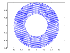
(a) $t=0$

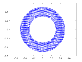
(b) $t=0.15$

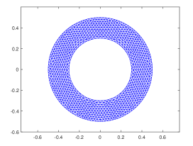
(c) $t=0.3$

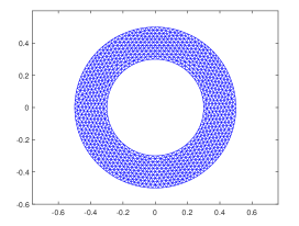
(d) $t=0.456$

Figure 3: Example 4.1. The mesh of $N=1998$ is plotted at $t=0$, 0.15, 0.3, and 0.456 for $\lambda=-2/\ln(0.6)$.

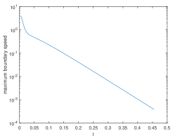
Figure 4: Example 4.1. The maximum boundary velocity is plotted as a function of time for $\lambda=-2/\ln(0.6)$ and $N=1998$.

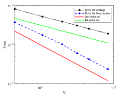
Figure 5: Example 4.1. The error in the boundary location is plotted as a function of $N$ (the number of elements in the mesh) for two strategies (the quadratic least squares fitting and area-weighted averaging) for computing solution gradient used in boundary update.

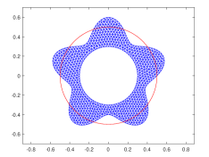
(a) $t=0$

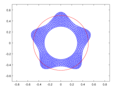
(b) $t=0.01$

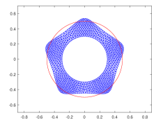
(c) $t=0.02$

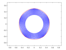
(d) $t=0.05$

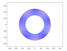
(e) $t=0.1$

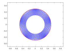
(f) $t=0.3$

Figure 6: Example 4.1. The mesh of $N=1567$ is plotted at $t=0$, 0.01, 0.02, 0.05, 0.1, and 0.3 for $\lambda=-2/\ln(0.6)$.

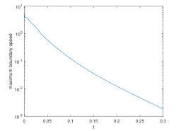
Figure 7: Example 4.1. The maximum boundary velocity is plotted as a function of time for $\lambda=-2/\ln(0.6)$ and $N=1567$.

      Example 4.2 (Exterior Bernoulli FBP with $T$-shape).

For this example, $\Gamma_{1}$ is taken as the boundary of the $T$-shape

$$(-3/8,3/8)\times(-1/4,0)\cup(-1/8,1/8)\times[0,1/4)$$

and the initial position of $\Gamma_{2}$ is a circle of radius 0.75. This problem was used by several researchers (e.g., see Eppler and Harbrecht [15]).

Fig. 8 shows the mesh at various time instants for $\lambda=5$. Fig. 9 shows that the maximum boundary velocity decreases as the time increases, implying that (2) has a steady-state solution for this example. Fig. 10 shows $\Gamma_{2}$ obtained for $\lambda=1$, 3, 5, 7 and 9. As $\lambda$ increases, $\Gamma_{2}$ is getting closer to $\Gamma_{1}$. The results obtained here are comparable with those in literature and particularly those obtained in [15] using a shape optimization method. ∎

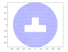
(a) $t=0$

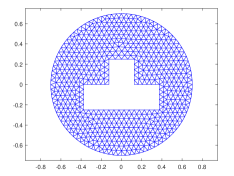
(b) $t=0.01$

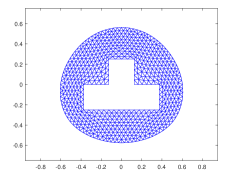
(c) $t=0.05$

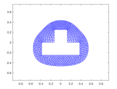
(d) $t=0.15$

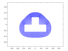
(e) $t=0.3$

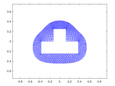
(f) $t=0.446$

Figure 8: Example 4.2. The mesh of $N=1259$ is plotted at $t=0$, 0.05, 0.1, 0.15, 0.3, and 0.446 for $\lambda=5$.

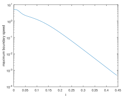
Figure 9: Example 4.2. The maximum boundary velocity is plotted as a function of time for $\lambda=5$ and $N=1259$.

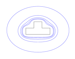
Figure 10: Example 4.2. $\Gamma_{2}$ obtained for $\lambda=1$, 3, 5, 7, and 9 with a mesh of $N=1259$.

      Example 4.3 (Exterior Bernoulli FBP with two disjoint shapes).

This example is selected from Rabago [36]. The interior boundary, $\Gamma_{1}$, consists of the boundary of two disjoint shapes

$$(1+0.7\cos(\theta)-0.4\cos(2\theta),\;\sin(\theta)),\;0\leq\theta\leq 2\pi$$

$$(-2+\cos(\theta)+0.4\cos(2\theta),\;0.5+0.7\sin(\theta)),\;0\leq\theta\leq 2\pi.$$

The initial position of $\Gamma_{2}$ is taken as a circle of radius 5 with center (0,0).

Figs. 11 and 12 show a mesh at various time instants and the maximum boundary velocity as a function of time, respectively. The location of $\Gamma_{2}$ obtained for several values of $\lambda$ is plotted in Fig. 13. The results show that the moving mesh FEM with the pseudo-transient continuation works well for this example with more complex $\Gamma_{1}$. Particularly, the mesh stays free of tangling for all computations. ∎

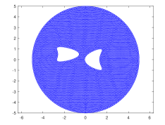
(a) $t=0$

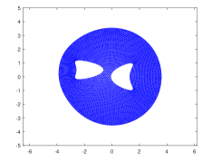
(b) $t=1$

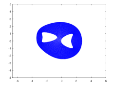
(c) $t=2$

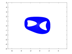
(d) $t=3$

(e) $t=6$

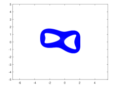
(f) $t=9.941$

Figure 11: Example 4.3. The mesh of $N=10630$ is plotted at $t=0$, 1, 2, 3, 6, and 9.941 for $\lambda=1.5$.

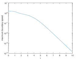
Figure 12: Example 4.3. The maximum boundary velocity is plotted as a function of time for $\lambda=1.5$ and $N=10630$.

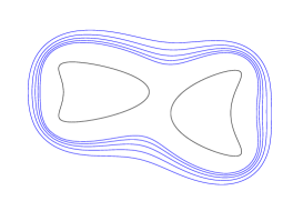
Figure 13: Example 4.4. The boundary $\Gamma_{2}$ is obtained with $\lambda=1.1$, 1.3, 1.5, 1.7 and 1.9 and a mesh of $N=10630$.

      Example 4.4 (Interior Bernoulli FBP with $L$-shape).

Finally, we consider an interior Bernoulli FBP. In this example, $\Gamma_{1}$ is taken as the boundary of the $L$-shape

$$(1,5.8)\times(1,9)\cup[5.8,9)\times(4.2,9)$$

and the initial position of $\Gamma_{2}$ is the circle of radius 1.5 with center (4.2, 6). A similar example was considered by Flucher and Rumpf [17] and several other researchers.

Fig. 14 shows the mesh at various time instants and Fig. 15 shows the maximum boundary velocity as a function of time. For this example, the solution converges more slowly to steady state than previous examples. The computation is stopped at $t=20$ when the maximum boundary velocity is about $2\times 10^{-2}$ and the boundary displacement is about $2\times 10^{-5}$. Nevertheless, the figures show that the maximum boundary velocity decreases steadily and $\Gamma_{2}$ is converging towards steady state. Fig. 16 shows $\Gamma_{2}$ for several values of $\lambda$. As $\lambda$ increases, $\Gamma_{2}$ is getting closer to $\Gamma_{1}$. The results are comparable with those in [17] where the explicit and implicit Neumann methods are used. ∎

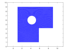
(a) $t=0$

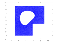
(b) $t=4$

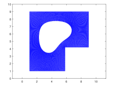
(c) $t=8$

(d) $t=10$

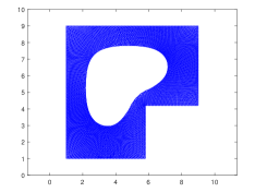
(e) $t=16$

(f) $t=20$

Figure 14: Example 4.4. The mesh of $N=11334$ is plotted at $t=0$, 4, 8, 10, 16, and 20 for $\lambda=0.9$.

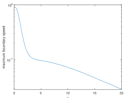
Figure 15: Example 4.4. The maximum boundary velocity is plotted as a function of time for $\lambda=0.9$.

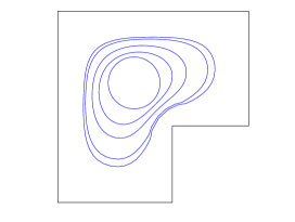
Figure 16: Example 4.4. The boundary $\Gamma_{2}$ is obtained with $\lambda=0.75$, 0.8, 0.85, 0.9 and 0.95.

5 Numerical examples for FBPs with non-constant Bernoulli condition and nonlinear FBPs

The moving mesh method described in Section 3 can be used for more general FBPs without major modifications. To demonstrate this, we present in this section numerical results for three examples, one with non-constant Bernoulli boundary condition, one with the $p$-Laplacian (nonlinear), and one being a nonlinear obstacle problem. FBPs with non-constant Bernoulli conditions and/or $p$-Laplacian have been studied by a number of researchers, e.g., see Acker and Meyer [1] and Henrot and Shahgholian [24]. Obstacle problems are a classical and important types of FBPs (e.g., see Ros-Oton [37]). The settings and values of the parameters used in the computation are the same as in the previous section.

      Example 5.1 (Exterior Bernoulli FBP with non-constant Bernoulli condition).

This example is the same as Example 4.1 except that a non-constant Bernoulli boundary condition is used,

$$\lambda=-\frac{2}{\ln(0.6)}\left(1-0.5\sin(10\arctan(\frac{y}{x})\right).$$ (23)

The initial position of $\Gamma_{2}$ is taken as the circle with radius 0.6. A mesh and the corresponding maximum boundary velocity are plotted in Figs. 17 and 18, respectively. One can see that the steady-state $\Gamma_{2}$ for this example is a wavy circle, which is different from a circle in Example 4.1. The results also show that the moving mesh FEM with the pseudo-transient continuation works well for this example. ∎

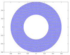
(a) $t=0$

(b) $t=0.15$

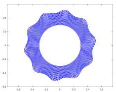
(c) $t=0.3$

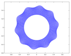
(d) $t=0.468$

Figure 17: Example 5.1. The mesh of $N=4618$ is plotted at $t=0$, 0.15, 0.3, and 0.468 for variable $\lambda$ (23).

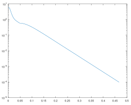
Figure 18: Example 5.1. The maximum boundary velocity is plotted as a function of time for variable $\lambda$ (23) and $N=4618$.

      Example 5.2 (Exterior Bernoulli FBP with $p$-Laplacian).

This example is the same as Example 4.2 except that the Laplace equation is replaced by the $p$-Laplace equation,

$$\nabla\cdot\big{(}|\nabla u|^{p-2}\nabla u\big{)}=0,\quad\text{ in }\Omega$$ (24)

where $p\in(1,\infty)$ is a parameter. The $p$-Laplacian is a power-law generalization of various linear flow laws and is more realistic than the Laplacian (e.g., see Acker and Meyer [1]). We take two values of $p$, $1.5$ and $5$, in our computation. The meshes obtained with $p=1.5$ and $p=5$ are shown in Figs. 19 and 20, respectively, and the corresponding maximum boundary velocities are plotted in Fig. 21. They confirm that the moving mesh FEM together with the pseudo-transient continuation works well for this nonlinear example. Moreover, Fig. 22 shows that the steady-state position of $\Gamma_{2}$ is more uniformly close to $\Gamma_{1}$ for larger $p$. ∎

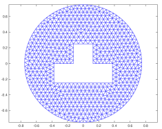
(a) $t=0$

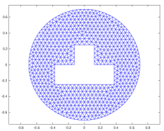
(b) $t=0.01$

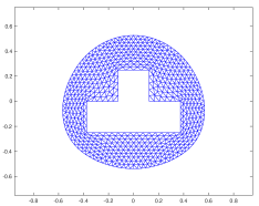
(c) $t=0.05$

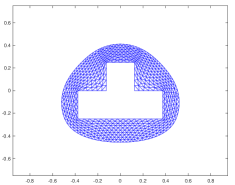
(d) $t=0.15$

(e) $t=0.3$

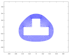
(f) $t=0.677$

Figure 19: Example 5.2 with $p=1.5$. The mesh of $N=1259$ is plotted at $t=0$, 0.05, 0.1, 0.15, 0.3, and 0.677 for $\lambda=5$.

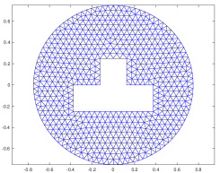
(a) $t=0$

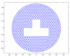
(b) $t=0.01$

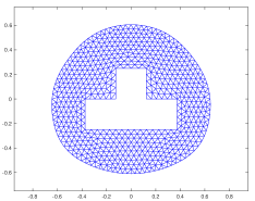
(c) $t=0.05$

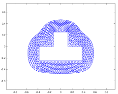
(d) $t=0.15$

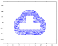
(e) $t=0.3$

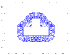
(f) $t=0.708$

Figure 20: Example 5.2 with $p=5.0$. The mesh of $N=1259$ is plotted at $t=0$, 0.05, 0.1, 0.15, 0.3, and 0.708 for $\lambda=5$.

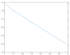
(a) $p=1.5$

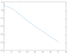
(b) $p=5.0$

Figure 21: Example 5.2. The maximum boundary velocity is plotted as a function of time for $\lambda=5$, $N=1259$, and two values of $p$.

(a) $p=1.5$

(b) $p=2.0$

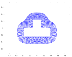
(c) $p=5.0$

Figure 22: Example 5.2 with $N=1259$ and $\lambda=5$. The mesh at $t=0.3$ is compared for $p=1.5$, $2.0$, and $5.0$.

      Example 5.3 (A nonlinear obstacle problem).

Obstacle problems are a classical and important type of free boundary problem where the solution can be thought as the equilibrium position of an elastic membrane that is constrained to lie above a given obstacle $\psi=\psi(\mbox{\boldmath$x$})$ while its boundary is held fixed (e.g., see Ros-Oton [37]). We consider here a nonlinear obstacle problem

$$\min_{u}\int_{D}\sqrt{1+|\nabla u|^{2}}d\mbox{\boldmath$x$},\quad\text{subject to}\quad u\geq\psi\text{ in }D,\quad u=\psi\text{ on }\partial D$$ (25)

where $D$ is the disk with radius $2$ and

$$\psi=\begin{cases}\sqrt{1-x^{2}-y^{2}},&\quad x^{2}+y^{2}\leq 1\\ 0,&\quad\text{otherwise}.\end{cases}$$

This problem can be reformulated into a free boundary problem as

$$\begin{cases}-\nabla\cdot\left(\frac{1}{\sqrt{1+|\nabla u|^{2}}}\nabla u\right)=0,&\quad\text{ in }\Omega\\ u=\psi,&\quad\text{ on }\Gamma_{1}=\partial D\\ u=\psi,&\quad\text{ on }\Gamma_{2}\\ \frac{\partial u}{\partial n}=\frac{\partial\psi}{\partial n},&\quad\text{ on }\Gamma_{2}\end{cases}$$ (26)

where $\Gamma_{2}$ is a closed curve inside $D$, $\Omega=D\setminus\overline{E}$, and $E$ is the domain enclosed by $\Gamma_{2}$. The Neumann boundary condition on $\Gamma_{2}$ is mathematically equivalent to a Bernoulli condition $|\nabla(u-\psi)|=0$. Moreover, the corresponding MBP in the pseudo-transient continuation is given by

$$\begin{cases}\frac{\partial u}{\partial t}=\nabla\cdot\left(\frac{1}{\sqrt{1+|\nabla u|^{2}}}\nabla u\right),&\quad\text{ in }\Omega\\ u=\psi,&\quad\text{ on }\Gamma_{1}=\partial D\\ u=\psi,&\quad\text{ on }\Gamma_{2}\\ \dot{\Gamma}=-\frac{\partial u}{\partial n}+\frac{\partial\psi}{\partial n},&\quad\text{ on }\Gamma_{2}.\end{cases}$$ (27)

The initial condition for $u$ is taken as $u(\mbox{\boldmath$x$},0)=0$ and the initial position of $\Gamma_{2}$ is chosen as the circle with radius 0.8. The mesh, solution, and maximum boundary velocity obtained with a mesh of $N=2264$ are plotted in Fig. 23. The results demonstrate that the moving mesh FEM and the pseudo-transient continuation can be used to obtain the solution of the nonlinear obstacle problem (25) as the steady-state solution of (27). ∎

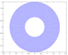
(a) mesh at $t=0$

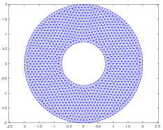
(b) mesh at $t=2.686$

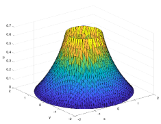
(c) solution at $t=2.686$

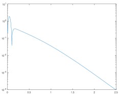
(d) max. boundary velocity vs $t$

Figure 23: Example 5.3. The results are obtained with a mesh of $N=2264$.

6 Conclusions and comments

We have studied a moving mesh finite element method for the numerical solution of Bernoulli FBPs. The method is based on the pseudo-transient continuation with which an MBP is constructed and its steady-state solution is taken as the solution of the underlying Bernoulli FBP. The MBP is solved in a split manner at each time step: the moving boundary is updated with the Euler scheme, the interior mesh points are moved using the MMPDE moving mesh method, and the corresponding initial-boundary value problem is solved using the linear FEM. The overall procedure is listed in Algorithm 1. The method can take full advantages of both the pseudo-transient continuation and the MMPDE method. Particularly, it is able to move the mesh, free of tangling, to fit the varying domain for a variety of geometries, no matter if they are convex or concave. Moreover, it is convergent towards steady state for a broad class of FBPs and initial guesses of the free boundary.

Numerical examples for Bernoulli FBPs with constant and non-constant Bernoulli conditions and nonlinear FBPs have been presented. Numerical results have shown that the method is second-order in space when the gradient of the solution at boundary vertices that is needed in free boundary update is recovered with quadratic least squares fitting. Moreover, they have also shown that the method works well for both exterior and interior Bernoulli FBPs with complex geometries and nonlinear FBPs.

Finally, we comment that while it is generally more robust than Newton’s method, the pseudo-transient continuation is typically slower than the latter (in terms of convergence towards steady state). Unfortunately, the moving mesh method studied in this work also inherits this drawback from the pseudo-transient continuation. It is interesting to see how the method can be sped up. One idea is to use a Davidenko-like equation or a preconditioner (e.g. see Kramer [30]) when constructing the moving boundary problem in the pseudo-transient continuation. A main challenge on this is how to speed up the movement of the free boundary while avoiding mesh tangling. Another issue is how to compute hyperbolic solutions [23]. As suggested by the formal analysis in Section 2 or Fig. 2, it seems that the pseudo-transient continuation and thus the moving mesh FEM studied in this work can be used only for elliptic solutions. It is interesting to see if a method based on the pseudo-transient continuation can be designed for computing hyperbolic solutions.

References

- [1] A. Acker and R. Meyer. A free boundary problem for the -Laplacian: uniqueness, convexity, and successive approximation of solutions. Elec. J. Diff. Eq. 1995 (1995), 1-20.
- [2] H. W. Alt and L. A. Cafarelli. Existence and regularity for a minimum problem with free boundary. J. Reine Angew. Math. 325 (1981), 105-144.
- [3] M. J. Baines, Moving Finite Elements, Oxford University Press, Oxford, 1994.
- [4] M. J. Baines, M. E. Hubbard, and P. K. Jimack, Velocity-based moving mesh methods for nonlinear partial differential equations, Comm. Comput. Phys. 10 (2011), 509-576.
- [5] A. Beurling. On free boundary problems for the Laplace equation. Seminars on Analytic functions, Institute for Advanced Study, Princeton, NJ, 1 (1957), 248-263.
- [6] W. Boscheri, M. Semplice, and M. Dumbser. Central WENO subcell finite volume limiters for ADER discontinuous Galerkin schemes on fixed and moving unstructured meshes. Commun. Comput. Phys. 25 (2019), 311-346.
- [7] R. Brügger, R. Croce, and H. Harbrecht. Solving a Bernoulli type free boundary problem with random diffusion. ESAIM: Cont. Opt. Cal. Var. 26 (2020), 56.
- [8] C. J. Budd, W. Huang, and R. D. Russell. Adaptivity with moving grids. Acta Numer. 18 (2009), 111-241.
- [9] E. Burman, D. Elfverson, P. Hansbo, M. G. Larson, and K. Larsson. A cut finite element method for the Bernoulli free boundary value problem. Comput. Methods Appl. Mech. Engrg. 317 (2017), 598-618.
- [10] P. Cardaliaguet and R. Tahraoui. Some uniqueness results for Bernoulli interior free-boundary problems in convex domains. Elec. J. Diff. Eq. 2002 (2002), 1-16.
- [11] F. Chen, B. Zheng, J. Lin, and W. Chen. Numerical solution of steady-state free boundary problems using the singular boundary method. Adv. Appl. Math. Mech. 13 (2021), 163-175.
- [12] J. Crank. Free and Moving Boundary Problems. Clarendon Press, New York, 1984.
- [13] Y. Du and Z. G. Lin. Spreading-vanishing dichotomy in the diffusive logistic model with a free boundary. SIAM J. Math. Anal. 42 (2010), 377-405.
- [14] K. Eppler and H. Harbrecht. Efficient treatment of stationary free boundary problems. Appl. Numer. Math. 56 (2006), 1326-1339.
- [15] K. Eppler and H. Harbrecht. Shape optimization for free boundary problems - analysis and numerics. Int. Ser. Numer. Math. 160 (2012), 277-288.
- [16] C. A. J. Fletcher. Computational Techniques for Fluid Dynamics 1, Fundamental and General Techniques. Springer-Verlag, Berlin, 1991.
- [17] M. Flucher and M. Rumpf. Bernoulli’s free-boundary problem, qualitative theory and numerical approximation. J. Reine Angew. Math. 486 (1997), 165-204.
- [18] A. Friedman and B. Hu. Asymptotic stability for a free boundary problem arising in a tumor model. J. Diff. Eq. 227 (2006), 598-639.
- [19] S. González-Pinto, J. I. Montijano, and S. Pérez-Rodríguez. Two-step error estimators for implicit Runge-Kutta methods applied to stiff systems. ACM Trans. Math. Software 30 (2004), 1-18.
- [20] Y. Gu, D. Luo, Z. Gao, and Y. Chen. An adaptive moving mesh method for the five-equation model. Commun. Comput. Phys. 32 (2022), 189-221.
- [21] J. Haslinger, T. Kozubek, K. Kunisch, and G. Peichl. Shape optimization and fictitious domain approach for solving free boundary problems of Bernoulli type. Comput. Opt. Appl. 26 (2003), 231-251.
- [22] J. Haslinger and R. A. E. Mäkinen. Introduction to Shape Optimization, Theory, Approximation, and Computation. The Society of Industrial and Applied Mathematics, Philadelphia, 2003.
- [23] A. Henrot and M. Onodera. Hyperbolic solutions to Bernoulli’s free boundary problem. Arch. Rational Mech. Anal. 240 (2021), 761-784.
- [24] A. Henrot and H. Shahgholian. The one phase free boundary problem for the -Laplacian with non-constant Bernoulli boundary condition. Trans. Amer. Math. Soc. 354 (2002), 2399-2416.
- [25] W. Huang. An introduction to MMPDElab. arXiv:1904.05535.
- [26] W. Huang and L. Kamenski. A geometric discretization and a simple implementation for variational mesh generation and adaptation. J. Comput. Phys. 301 (2015), 322-337.
- [27] W. Huang and L. Kamenski. On the mesh nonsingularity of the moving mesh PDE method. Math. Comp. 87 (2018), 1887-1911.
- [28] W. Huang, Y. Ren, and R. D. Russell. Moving mesh partial differential equations (MMPDEs) based upon the equidistribution principle. SIAM J. Numer. Anal. 31 (1994), 709-730.
- [29] W. Huang and R. D. Russell. Adaptive Moving Mesh Methods. Springer, New York, 2011. Applied Mathematical Sciences Series, Vol. 174.
- [30] M. E. Kramer. Aspects of solving non-linear boundary value problems numerically, PhD Thesis, 1992, Technische Universiteit Eindhoven.
- [31] C. M. Kuster, P. A. Gremaud, and R. Touzani. Fast numerical methods for Bernoulli free boundary problems. SIAM J. Sci. Comput. 29 (2007), 622-634.
- [32] C. M. Murea and G. Hentschel. Finite element methods for investigating the moving boundary problem in biological development. Prog. Nonlin. Diff. Eq. Appl. 64 (2005), 357-371.
- [33] C. Ngo and W. Huang. Adaptive finite element solution of the porous medium equation in pressure formulation. Numer. Meth. Part. Diff. Eq. 35 (2019), 1224-1242.
- [34] R. Rangarajan and A. J. Lew. Analysis of a method to parameterize planar curves immersed in triangulations. SIAM J. Numer. Anal. 51 (2013), 1392-1420.
- [35] R. Rangarajan and A. J. Lew. Universal meshes: A method for triangulating planar curved domains immersed in nonconforming triangulations. Int. J. Numer. Meth. Eng. 98 (2014), 236-264.
- [36] J. F. T. Rabago. Analysis and numerics of novel shape optimization methods for the Bernoulli problem. Nagoya University, 2020. PhD Thesis.
- [37] X. Ros-Oton. Obstacle problems and free boundaries: an overview. SeMA 75, (2018), 399-419.
- [38] J. Sokolowski and J.-P. Zolesio. Introduction to Shape Optimization, Shape Sensitivity Analysis. Springer-Verlag, Berlin, 1992.
- [39] K. Sturm. On shape optimization with non-linear partial differential equations. Technical University of Berlin, 2015, PhD Thesis.
- [40] Y. Sunayama, M. Kimura, and J. Rabago. Comoving mesh method for certain classes of moving boundary problems. Japan J. Indust. Appl. Math. 39 (2022), 973-1001.
- [41] T. Tang, Moving mesh methods for computational fluid dynamics flow and transport, Recent Advances in Adaptive Computation (Hangzhou, 2004), Volume 383 of AMS Contemporary Mathematics, pages 141-173. Amer. Math. Soc., Providence, RI, 2005.
- [42] G. S. Weiss. Bernoulli type free boundary problems and water waves. in Geometric Measure Theory and Free Boundary Problems, edited by M. Focardi and E. Spadaro, pp. 89-136, 2021, Springer, Lecture Notes in Mathematics Vol. 2284.
- [43] E. S. Wise, B. T. Cox, and B. E. Treeby. Mesh density functions based on local bandwidth applied to moving mesh methods. Commun. Comput. Phys. 22 (2017), 1286-1308.
- [44] Y. Yamada. Asymptotic properties of a free boundary problem for a reaction-diffusion equation with multi-stable nonlinearity. Rend. Istit. Mat. Univ. Trieste 52 (2020), 65-89.
- [45] M. Zhang, W. Huang, and J. Qiu. A well-balanced positivity-preserving quasi-Lagrange moving mesh DG method for the shallow water equations. Comm. Comput. Phys. 31 (2022), 94-130.
- [46] F. Zhou, J. Wu, and S. Cui. Existence and asymptotic behavior of solutions to a moving boundary problem modeling the growth of multi-layer tumors. Comm. Pure Appl. Anal. 8 (2009), 1669-1688.