QCD Predictions for Meson Electromagnetic Form Factors at High Momenta:
Testing Factorization in Exclusive Processes

Abstract

We report the first lattice QCD computation of pion and kaon electromagnetic form factors, $F_{M}(Q^{2})$, at large momentum transfer up to 10 and 28 $\mathrm{GeV}^{2}$, respectively. Utilizing physical masses and two fine lattices, we achieve good agreement with JLab experimental results at $Q^{2}\lesssim 4~{}\mathrm{GeV}^{2}$. For $Q^{2}\gtrsim 4~{}\mathrm{GeV}^{2}$, our results provide ab-initio QCD benchmarks for the forthcoming experiments at JLab 12 GeV and future electron-ion colliders. We also test the QCD collinear factorization framework utilizing our high-$Q^{2}$ form factors at next-to-next-to-leading order in perturbation theory, which relates the form factors to the leading Fock-state meson distribution amplitudes. Comparisons with independent lattice QCD calculations using the same framework demonstrate, within estimated uncertainties, the universality of these nonperturbative quantities.

I Introduction

Elastic electron hadron scattering can be described in terms of electromagnetic form factors (EMFF), which characterize the charge distribution inside hadrons [1]. The EMFF of the nucleon has been studied experimentally for many decades and provided the first glimpse of the complex internal structure of the nucleon [2], while the EMFF of pion and kaon, the Goldstone bosons of QCD, are much less known. On the other hand, the study of the pion and kaon EMFF is important for at least two reasons. It has been argued that the pion and kaon form factors are important for understanding the dynamical generation of hadron masses in QCD [3, 4], and they are closely related to the light-front wave functions of the pseudo-scalar mesons, see, e.g., Ref. [5]. Studies of the pion and kaon electromagnetic form factors at large momentum transfer, $Q^{2}$, and, more generally, of the hard exclusive processes are needed for a more complete understanding of the partonic structure of the hadrons. The partonic picture of hadrons is well established through the study of inclusive processes, but we need to see that this picture also works in exclusive processes for an unambiguous interpretation of partons as the right degrees of freedom at short distances. While QCD factorization and the associated parton picture are well established in hard inclusive processes, this is not the case for hard exclusive processes. The QCD factorization for hard exclusive processes was proposed a long time ago [6, 7], but it could not be tested experimentally due to a lack of experimental data. The factorization in exclusive processes is key for the study of semi-leptonic decays of the $B$ mesons, which is important for testing the Standard Model, see, e.g., Refs. [8, 9].

Direct experimental measurements of the pion EMFF are available only for very small $Q^{2}$, well below $1~{}{\rm GeV}^{2}$ [10, 11, 12, 13]. It is possible to determine the pion form factor at higher $Q^{2}$ through pion electro-production off nucleons, but such determination comes with some model dependence [14]. However, also the measurements using this method do not extend to high enough values of $Q^{2}$. Measuring the kaon EMFF is even more challenging [15, 16, 17, 18]. Studies of the EMFF of the pion and kaon with high $Q^{2}$ up to $\sim$ 6 $\rm GeV^{2}$ are underway at the ongoing JLAB 12 GeV program [19, 20], and their measurements in an extended range of $Q^{2}\sim$ 9$-$40 $\rm GeV^{2}$ are planned at the future Electron-Ion Collider (EIC) facility [21] and Electron-ion collider in China (EicC) [22].

At present, lattice QCD is the only nonperturbative method that can directly predict EMFF without any model dependence, and the results can also be systematically improved. Therefore, first-principle calculations on a lattice can provide benchmark QCD predictions for comparison with experiments. Existing lattice calculations of the pion [23, 24, 25, 26, 27, 28, 29, 30] and kaon [31, 32] EMFF are restricted to the low $Q^{2}$ region. Calculations of pion EMFF with $Q^{2}$ up to 6 $\rm GeV^{2}$ were performed in Ref. [33] using the Feynman-Hellmann method, albeit with large uncertainties. In this work, we study the pion and kaon EMFF with large momentum transfers $Q^{2}$ up to 10 $\rm GeV^{2}$ and 28 $\rm GeV^{2}$, respectively, using optimized boosted sources for large momenta in both the initial and final states. Moreover, with independent lattice QCD calculations of the pion and kaon light-cone distribution amplitudes [34, 35, 36], as well as the state-of-the-art perturbative input at next-to-next-to-leading order (NNLO) [37], we are able to verify the collinear leading-twist QCD factorization of the EMFF at such high $Q^{2}$ [6, 7] for the first time, thus demonstrating the universality within these nonperturbative quantities.

II Lattice QCD calculations of the form factors

We extract the bare meson form factors from meson two-point and meson-current three-point correlation functions. We use two lattice QCD gauge ensembles generated by the HotQCD collaboration [38] with 2+1 flavors of highly improved staggered quarks (HISQ) [39]. These ensembles are defined on $L_{s}^{3}\times L_{t}=64^{3}\times 64$ lattices with spacings $a=0.076$ fm and 0.04 fm. The strange quark mass $m_{s}$ for these ensembles is set to the physical value while the light quark masses are set to $m_{s}/27$ and $m_{s}/20$, respectively. The light quark masses correspond to the pion masses of 140 MeV and 160 MeV for the coarser and the finer lattice, respectively. For the valence quarks, we use the Wilson-clover action with 1-step hypercubic (HYP) smeared [40] gauge links and with tree-level tadpole improved coefficients $c_{sw}$ = 1.0372 and 1.02868 [41, 42] for the coarser and the finer lattices, respectively, which were determined from the smeared plaquette averages. The valence quark masses are tuned so that the pion/kaon masses are 140(1)/498(1) MeV for the $a$ = 0.076 fm ensemble and 134(3)/497(4) MeV for the $a$ = 0.04 fm ensemble. We use the QUDA multigrid algorithm [43, 44, 45, 46] for the Wilson-Dirac operator inversions to calculate the quark propagators. All Mode Averaging (AMA) technique [47] is employed to increase the statistics.

In order to obtain the bare matrix elements of the ground state, we need to compute the two-point functions to extract the energy spectra and get the overlap amplitudes,

$$C_{\rm 2pt}(\mathbf{P},t_{s})=\left\langle[\Pi_{S}(\mathbf{P},t_{s})][\Pi_{S}(\mathbf{P},0)]^{\dagger}\right\rangle.$$ (1)

Here, $\Pi_{S}=\pi_{S},K_{S}$ denote the pion and kaon interpolating operators, respectively, which can be written as follows,

$$\begin{split}\pi_{S}(\mathbf{P},t)=&\sum_{\mathbf{x}}\bar{d}_{S}(\mathbf{x},t)\gamma_{5}u_{S}(\mathbf{x},t)e^{-i\mathbf{P}\cdot\mathbf{x}},\\ K_{S}(\mathbf{P},t)=&\sum_{\mathbf{x}}\bar{s}_{S}(\mathbf{x},t)\gamma_{5}u_{S}(\mathbf{x},t)e^{-i\mathbf{P}\cdot\mathbf{x}}.\\ \end{split}$$ (2)

These interpolating operators are constructed from Gaussian-smeared quark sources (sinks) in Coulomb gauge [48], which are also boosted with momentum $\mathbf{k}^{i}$ ($\mathbf{k}^{f}$) [49, 48]. Hence, we use the subscript $S$ in the above equations. The Gaussian radii of the light and strange quarks used in this work are $r_{l}^{G}$ = 0.59 fm and $r_{s}^{G}$ = 0.83 fm for the $a$ = 0.076 fm lattice, and $r_{l}^{G}$ = 0.59 fm and $r_{s}^{G}$ = 0.86 fm for the $a$ = 0.04 fm lattice.

The three-point functions for EMFF can be written as

$$C_{\rm 3pt}(\mathbf{P}^{f},\mathbf{P}^{i};\tau,t_{s})=\left\langle[\Pi_{S^{f}}(\mathbf{P}^{f},t_{s})]O_{\Gamma}(\mathbf{q},\tau)[\Pi_{S^{i}}(\mathbf{P}^{i},0)]^{\dagger}\right\rangle,$$ (3)

with $\mathbf{P}^{i}=\mathbf{P}^{f}-\mathbf{q}$. Here, the electro-magnetic current is $O_{\Gamma}=\frac{2}{3}\bar{u}\gamma_{\mu}u-\frac{1}{3}\bar{d}\gamma_{\mu}d$ and $\frac{2}{3}\bar{u}\gamma_{\mu}u-\frac{1}{3}\bar{s}\gamma_{\mu}s$ for pion and kaon, respectively. The time component of the vector current $\gamma_{\mu}=\gamma_{0}$ is used. With degenerate light quark masses, there are no disconnected diagrams for the pion, while their contribution to the kaon, which is expected to be small, is neglected in this work. To achieve high momentum transfer $Q^{2}=-(p^{f}-p^{i})^{2}$ as the main target of this work, we make use of the Breit frame with $\mathbf{P}^{f}=(0,0,-P_{3})$ and $\mathbf{q}=(0,0,-2P_{3})$, when calculating the three-point functions. Here $P_{3}=2\pi n_{3}/(L_{s}a)$ with $n_{3}$ being an integer. To optimize the signal, we use the same quark boost parameter $\zeta$ for the hadron states moving back-to-back, meaning that for the quark momentum boost, we choose $\mathbf{k}^{f}$ = $-\mathbf{k}^{i}$ to ensure $\zeta=\mathbf{k}^{i}/\mathbf{P}^{i}=\mathbf{k}^{f}/\mathbf{P}^{f}$  [41, 42]. Given that the hadron states with slight momentum variation share the same propagator [41], it is possible to reliably calculate the three-point functions at multiple momentum transfers with small deviations from the Breit frame, requiring minimal additional computational costs. For instance, in the case of the kaon, apart from the Breit frame scenario with $\mathbf{P}^{f}=(0,0,-2.42)$ GeV and $\mathbf{P}^{i}=(0,0,2.42)$ GeV, we can also consider the non-Breit frame setup with $\mathbf{P}^{f}=(0,0,-2.42)$ GeV and $\mathbf{P}^{i}=(0,0,2.91)$ GeV, which allows us to reach $Q^{2}$ up to $28~{}\mathrm{GeV}^{2}$. In this study, we used 350 gauge configurations for the $a=0.076$ fm lattice and 280 gauge configurations for the $a=0.04$ fm lattice. The number of AMA samples ranged from 32 to 256, depending on the lattice spacing and the momentum considered, with more samples used for larger momenta. More detailed information on our choice of momenta and the number of AMA samples can be found in the Appendix.

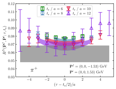
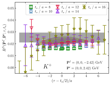
Figure 1: Left panel: ratios $R^{fi}(t_{s},\tau)$ for the pion with $Q^{2}=9.4~{}\rm GeV^{2}$ from the $a=0.076$ fm lattice. Right panel: ratios $R^{fi}(t_{s},\tau)$ for the kaon with $Q^{2}=23.4~{}\rm GeV^{2}$ from the $a=0.04$ fm lattice. The colored bands denote the two-state fit results of the corresponding colored lattice data, and the grey bands display the bare matrix elements of the ground state.

To take advantage of the correlation between the two-point and three-point functions, we construct the ratio

$$R^{fi}(\mathbf{P}^{f},\mathbf{P}^{i};\tau,t_{s})\equiv\frac{2\sqrt{E_{0}^{f}E_{0}^{i}}}{E_{0}^{f}+E_{0}^{i}}\frac{C_{\rm 3pt}(\mathbf{P}^{f},\mathbf{P}^{i};\tau,t_{s})}{C_{\rm 2pt}(\mathbf{P}^{f},t_{s})}\left[\frac{C_{\rm 2pt}(\mathbf{P}^{i},t_{s}-\tau)C_{\rm 2pt}(\mathbf{P}^{f},\tau)C_{\rm 2pt}(\mathbf{P}^{f},t_{s})}{C_{\rm 2pt}(\mathbf{P}^{f},t_{s}-\tau)C_{\rm 2pt}(\mathbf{P}^{i},\tau)C_{\rm 2pt}(\mathbf{P}^{i},t_{s})}\right]^{1/2}.$$ (4)

In the $t_{s}\rightarrow\infty$ limit, this ratio approaches the ground-state bare matrix elements $R^{fi}(\mathbf{P}^{f},\mathbf{P}^{i};\tau\rightarrow\infty,t_{s}\rightarrow\infty)=F^{B}_{M}(Q^{2})$ ($M=\pi^{+}$ or $K^{+}$). Taking the results of the energy levels and overlap amplitudes from the analysis of the two-point functions, we use the two-state fit on the lattice data to extract the bare matrix elements from the ratios. Details of the analysis can be found in the Appendix. We show examples in the Breit frame of the ratio $R^{fi}$ in Fig. 1 for the pion at $Q^{2}=9.4~{}\rm GeV^{2}$ on the $a=0.076$ fm lattice (left panel) and the kaon at $Q^{2}=23.4~{}\rm GeV^{2}$ on the $a=0.04$ fm lattice (right panel). Despite the very large momentum transfer, reasonable signals can be obtained by using the optimized boosted sources and large statistics. The bands in the figure show the results of the two-state fit with the corresponding statistical errors obtained from the bootstrap analysis. As one can see from the figure, the fit results describe the data very well. The grey bands display the results at the limits of infinite source-sink separation, giving the bare matrix elements of the pion and kaon ground states, that is, the bare form factors. These bare matrix elements $F^{B}_{M}(Q^{2})$ are then converted to physical form factor values $F_{M}(Q^{2})=Z_{V}F^{B}_{M}(Q^{2})$ using the vector current renormalization factors $Z_{V}$. We use the values of $Z_{V}$ calculated in our previous studies [42, 30] employing the same lattice setups, specifically $1/Z_{V}$ = 1.048(2) and 1.024(1) for the $a=0.076$ fm and 0.04 fm lattices, respectively.

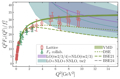
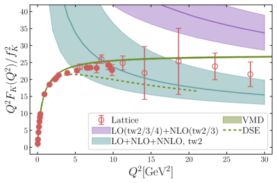
Figure 2: The renormalized EMFF of the pion (left panel) and kaon (right panel) are shown as $Q^{2}F_{M}(Q^{2})/f^{2}_{M}$. For the case of pion, we include the low $Q^{2}$ results (filled square symbols) from Ref. [30] that uses the same lattice setup, as well as the results from $F_{\pi}$ collaboration [50] extracted from the experimental data (open triangle symbols). For the case of kaon, we show the results from two different lattices with $a=0.076$ fm (filled circle symbols) and $a=0.04$ fm (open circle symbols). The blue bands represent the twist two (tw2) pQCD results using the collinear factorization at NNLO. The purple bands denote the pQCD results obtained within the $k_{T}$ factorization theorem, which includes higher-twist contributions from Refs. [51, 52, 53]; see text. The width of the band presents the perturbative uncertainty. In the case of the NNLO twist two results, it corresponds to the scale variation from $\mu=Q/2$ to $\mu=2Q$ and also includes the uncertainties of the conformal moments of the pion and kaon DA; see text. The green bands show the predictions with the VMD model by the fit on the lattice data at the low $Q^{2}$ region; see text. The dashed lines display the predictions from the DSE [54], BSE21 [55] and BSE24 [56]; see text.

III Form factors from low to high $Q^{2}$

Our results of the renormalized EMFF for the pion and the kaon are shown in Fig. 2 as the combination $Q^{2}F_{M}(Q^{2})/f^{2}_{M}$, where $f_{M}$ is the meson decay constant for $M=\pi^{+}$ or $K^{+}$, the reason for this combination will become clear below. We use the following values of the pion and kaon decay constant from FLAG21 [57, 58, 59, 60]: $f_{\pi}=130.2$ MeV and $f_{K}=155.7$ MeV. For the pion, we also show the lattice results at low $Q^{2}$ (BNL21) from Ref. [30] obtained using the same lattice setup with $a$ = 0.076 fm. Furthermore, in the left panel of the figure, we compare the lattice results on $F_{\pi^{+}}(Q^{2})$ to the experimental results from $F_{\pi}$ collaboration [50]. Impressively, the lattice determination exhibits excellent agreement with the experimental data. This agreement is reassuring for the model-based extraction of meson EMFF from experimental data, further bolstering the anticipation for their future experimental determination at JLAB [19, 20], EIC [21], and EicC [22]. For the kaon, we have results from two different lattice ensembles with $a=0.076$ fm (filled circle symbols) and $a=0.04$ fm (open circle symbols), which appear to be consistent at the overlap range. This suggests that the lattice artifacts are small compared to the statistical errors. Overall, one can observe that both $Q^{2}F_{\pi^{+}}(Q^{2})$ and $Q^{2}F_{K^{+}}(Q^{2})$ exhibit a rapid rise at low $Q^{2}$, transitioning into a plateau-like region at high $Q^{2}\gtrsim 5\rm~{}GeV^{2}$ within the errors.

At high $Q^{2}$, the asymptotic nature of QCD allows the factorization of the electromagnetic form factors into the convolutions of the meson DA and a hard-scattering kernel, as has been pointed out in the past [61, 6, 7]. Therefore, our lattice QCD results can be utilized to test this factorization. At the leading twist, the collinear factorization formula of the form factor reads

$$F_{M}(Q^{2})=\int^{1}_{0}\int^{1}_{0}dxdy\ \Phi^{*}_{M}(y,\mu^{2}_{F})T_{H}(x,y,Q^{2},\mu^{2}_{R},\mu^{2}_{F})\Phi_{M}(x,\mu^{2}_{F}),$$ (5)

where $T_{H}$ is the hard-process kernel calculated in perturbative QCD (pQCD). The hard kernel depends on the momentum transfer $Q^{2}$, the factorization scale $\mu_{F}$, as well as the renormalization scale $\mu_{R}$ at a fixed order of perturbation theory. It has been known up to the next-to-leading order (NLO) [62, 63, 64, 65] for some time. Very recently, the NNLO correction has become available [37]. The nonperturbative physics is encoded in the meson DA $\Phi_{M}(x,\mu^{2}_{F})$. Its dependence on $\mu_{F}$ comes from its anomalous dimension, which is compensated by the $\mu_{F}$-dependence of the hard kernel in the factorization formula above. The limit of very large $Q^{2}$ also implies that $\mu_{F}\rightarrow\infty$, and in this limit, one can use the asymptotic limit of DA, given by $\Phi_{M}^{\rm as}=3f_{M}x(1-x)/\sqrt{2N_{c}}$ ($N_{c}=3$ for QCD). Therefore, at asymptotically large $Q^{2}$, where the leading order (LO) result for $T_{H}$ is justified, we have $F_{M}(Q^{2}\rightarrow\infty)=8\pi\alpha_{s}(Q^{2})f_{M}^{2}/Q^{2}$. This means that $Q^{2}F_{M}(Q^{2})/f_{M}^{2}$ should be approximately constant and small at sufficiently large $Q^{2}$, explaining our normalization process. This LO asymptotic result gives a very small EMFF in comparison to the experimental results. For example, for the largest $Q^{2}=2.45~{}{\rm GeV}^{2}$ accessible experimentally, the LO asymptotic result predicts $Q^{2}F_{\pi^{+}}(Q^{2})/f_{\pi}^{2}\simeq 8.6$, which is almost three times smaller than the experimental value, as shown in Fig. 2.

The pion and kaon EMFF have also been calculated using the $k_{T}$ factorization approach [66, 67, 68, 51, 52]. For $Q\gg k_{T}$, the pion and kaon EMFF can also be related to the meson DA in this approach. Furthermore, it has long been suggested that higher-twist contributions to the EMFF factorization could be numerically large even for $Q^{2}<100$ GeV² despite being formally suppressed [69, 70, 71, 72, 68, 51, 52]. The state-of-the-art studies that consider higher-twist contributions are performed within the $k_{T}$ factorization approach and include all two- and three-particle (parton) contributions up to twist four [51, 52]. In Fig. 2, we compare our lattice results with the state-of-the-art perturbative calculations, including the higher-twist contributions under the $k_{T}$ factorization framework [51, 52, 53], as well as the pQCD predictions up to NNLO within the collinear factorization framework [37]. For the comparison with the lattice QCD results, we use the NNLO perturbative results written in terms of Gegenbauer expansion up to the sixth conformal moment. We have determined the pion and kaon DA on the $a$=0.076 fm lattice [35, 36], from which we obtain the conformal moments: $a_{2}=0.196(32),~{}a_{4}=0.085(26),~{}a_{6}=0.056(15)$ for the pion [35] and $a_{2}=0.134(22),~{}a_{4}=0.065(12),~{}a_{6}=0.035(7)$ for the kaon [36]. We use $\mu_{F}=\mu_{R}=\mu$, and vary $\mu$ between $Q/2$ and $2Q$.

We see from Fig. 2 that for $Q^{2}>5~{}{\rm GeV}^{2}$ lattice QCD results for pion and kaon EMFF agree with the collinear NNLO pQCD results within the estimated errors. For the pion, we also find agreement with NLO results from the $k_{T}$ factorization that includes higher-twist contributions [51, 52]. However, for the kaon case, the $k_{T}$ factorization approach with higher-twist contributions overestimates the lattice QCD results and also leads to much stronger $Q^{2}$-dependence of $Q^{2}F_{K}(Q^{2})$ compared to our lattice results.

The fact that LO asymptotic pQCD prediction results in small EMFF at large $Q^{2}$ in comparison to the experimental results, motivated the development of partonic approaches that incorporate some nonperturbative information. These approaches include those based on the Dyson-Schwinger equation (DSE) [54] and the Bethe-Salpeter equation (BSE) [55, 56]. The former approach is related to the idea of dynamical mass generation in QCD. We also compare our lattice results against these theoretical predictions in Fig. 2. For the pion EMFF, there is a reasonable agreement between the lattice QCD results and the DSE calculations [54], whereas the BSE calculations [55, 56] fall below the lattice results for $Q^{2}\gtrsim 3$ GeV². In the case of the kaon EMFF, there is some tension between the DSE calculations and the lattice results during the intermediate $Q^{2}$ range.

At low $Q^{2}$, the form factors could be understood by low-energy models such as the Vector Meson Dominance (VMD) model [73, 74]. Based on the lowest-lying vector resonances, the kaon form factors can be parameterized as [74, 75, 76]

$$F_{K^{+}}(Q^{2})=\sum_{v}\frac{c_{v}}{1+Q^{2}/m_{v}^{2}},$$ (6)

with $m_{v}$ being the mass of vector mesons. In this work, we take $v=\rho,\phi,\omega$ with their mass from PDG [77] and fit $c_{v}$ using the lattice results at low $Q^{2}\leq 0.4\rm~{}GeV^{2}$. Using this parameterization, the charge radius of $K^{+}$ can be determined by the slope at $F_{K^{+}}(0)$, which gives $\langle r^{2}_{K}\rangle=0.360(2)$ fm². This value is consistent with a recent dispersive analysis of the experimental data that gives $\langle r^{2}_{K}\rangle=0.359(3)$ fm² [76]. As for the pion, the form factors at low $Q^{2}$ can be parameterized by a single term in Eq. (6) using the VMD form, which is a one-parameter fit as discussed in Ref. [30]. The fit results from the VMD model extended to a high $Q^{2}$ region are also shown in Fig. 2. Surprisingly, the VMD fits from the low $Q^{2}$ region give a fairly good description of the lattice results for the pion and kaon EMFF, even for relatively large $Q^{2}$ values, up to $Q^{2}=5~{}{\rm GeV}^{2}$.

Since we have information on the pion and kaon form factors up to high $Q^{2}$, we can extract the charge or flavor distribution of hadrons in the impact parameter plane [78] using a model-independent way. There is no need to model the high $Q^{2}$ behavior of the form factors. We find that the impact parameter ($b_{\perp}$) distributions of the $u$ quark inside the pion and the kaon are identical. The distribution of the heavier $s$ anti-quark, on the other hand, is considerably narrower. The details of these calculations are presented in the Appendix.

IV Summary

In this work, we calculated the electromagnetic form factors of the pion and kaon with large $Q^{2}$ up to $10~{}\rm GeV^{2}$ and $28~{}\rm GeV^{2}$, respectively, on the lattice for the first time. For the kaon EMFF, we employ two lattice ensembles and find that the lattice artifacts are minor compared to the statistical uncertainties. Our results can serve as benchmark QCD predictions for model-based studies and for the forthcoming experimental measurements planned at JLab and the future EIC and EicC. We find that for $Q^{2}>5~{}{\rm GeV}^{2}$, the lattice results on the pion and kaon EMFF agree with the leading-twist collinear factorization if the NNLO hard kernel is used together with the most recent lattice QCD results on the DA. For smaller values of $Q^{2}$, our lattice QCD results can be understood in terms of the VMD model, suggesting that the transition from hadronic description to partonic description does not lead to abrupt changes in the $Q^{2}$-dependence of the pion and kaon EMFF. Finally, our results for the form factors provide a model-independent picture of the spatial distribution in the transverse plane of the up and strange quarks inside the pion and the kaon.

Appendix A The electromagnetic form factors of pion and kaon

The values of the momenta of the initial and final meson states used in this study are summarized in Table 1. On a finite lattice, the initial and final momenta are given as $\mathbf{P}^{i,f}=2\pi/(L_{s}a)\mathbf{n}^{i,f}_{\mathbf{P}}$, with $a$ being the lattice spacing and $L_{s}$ being the spatial grid size. The different choices of $\mathbf{n}^{i,f}$ are listed in Table 1. For each choice of $\mathbf{n}^{i,f}$, we list the corresponding quark boost momentum along the $z$ direction $k_{3}^{i,f}=2\pi/(L_{s}a)n_{k_{3}}^{i,f}$ for the initial and final states, as well as the momentum transfer $Q^{2}$. Additionally, we give the number of the exact and sloppy AMA samples.

The lattice results of the pion and kaon EMFF derived in this work are summarized in Table 2 and Table 3, respectively, which are also shown in Fig. 3 as a function of $Q^{2}$. For the case of pion, we also include the results from BNL21 [30] using the same lattice setup of the $a$ = 0.076 fm ensemble. For the case of kaon, we have two different lattice ensembles. Moreover, we also calculated the form factors of the valence quark. The results are shown in Fig. 4 along with the corresponding first-order spline interpolations. Using the spline interpolations, we can perform the numerical Fourier transformation of the valence quark form factors and obtain the distribution of $u$ quark inside the pion and kaon, as well as the distribution of $s$ anti-quark inside kaon in the transverse plane, i.e., distribution of valence quark in $b_{\perp}$. Here $b_{\perp}$ is the conjugate variable to $Q$ [78], and we used $Q^{2}$ up to 10 $\rm GeV^{2}$ for both pion and kaon for consistency. These distributions in the transverse plane are shown in the right panel of Fig. 4. We see that the valence $u$ quark $b_{\perp}$ distributions in pion and kaon are about the same, while the distribution of $s$ anti-quark is narrower.

Table 1: The values of the meson initial and final momenta used in this work and the numbers of the samples used in the AMA method are shown. The initial and final momenta and their corresponding boost parameters in the $z$-direction in units of $2\pi/(L_{s}a)$ are denoted by $\mathbf{n}^{i,f}_{\mathbf{P}}$ and $n^{i,f}_{k_{3}}$, respectively. The values of the momentum transfer $Q^{2}$ are given in physical units. Additionally, we provide the exact counts for both exact (#ex) and sloppy (#sl) inversion samples per configuration.

Meson	$a$[fm]	$\mathbf{n}^{f}_{\mathbf{P}}=(n^{f}_{P_{1}},n^{f}_{P_{2}},n^{f}_{P_{3}})$	$n^{f}_{k_{3}}$	$\mathbf{n}^{i}_{\mathbf{P}}=(n^{i}_{P_{1}},n^{i}_{P_{2}},n^{i}_{P_{3}})$	$n^{i}_{k_{3}}$	$Q^{2}$[GeV2]	(#ex, #sl)
Pion	$0.076$	(0, 0, -3)	-2	(0,0,2)	2	1.56	(3, 96)
				(0,0,3)		2.34
				(0,0,4)		3.12
				(2,0,3)		2.58
		(0, 0, -5)	-4	(0,0,3)	4	3.90	(7, 224)
				(0,0,4)		5.20
				(0,0,5)		6.50
				(2,0,4)		5.50
				(2,0,5)		6.75
		(0, 0, -6)	-5	(0,0,5)	5	7.80	(18, 576)
				(0,0,6)		9.35
				(2,0,5)		8.10
				(2,0,6)		9.61
Kaon	0.076	(0, 0, -1)	0	(0,0,1)	0	0.26	(1, 32)
				(1,0,-1)		0.062
				(1,0,0)		0.13
				(1,0,1)		0.32
				(1,1,0)		0.19
				(1,1,1)		0.38
		(0, 0, -3)	-2	(0,0,-2)	2	0.025	(5, 160)
				(0,0,1)		0.91
				(0,0,2)		1.58
				(0,0,3)		2.34
				(1,1,3)		2.46
				(2,2,3)		2.80
		(0, 0, -5)	-4	(0,0,3)	4	3.95	(8, 256)
				(0,0,4)		5.21
				(0,0,5)		6.50
				(1,1,5)		6.62
				(2,2,5)		6.98
		(0, 0, -6)	-6	(0,0,5)	6	7.80	(8, 256)
				(0,0,6)		9.35
				(1,1,6)		9.48
				(2,2,6)		9.84
	0.04	(0, 0, -3)	-2	(0,0,2)	2	5.66	(4, 128)
				(0,0,3)		8.44
				(0,0,4)		11.27
				(0,0,5)		14.13
		(0, 0, -5)	-4	(0,0,4)	4	18.77	(8, 256)
				(0,0,5)		23.45
				(0,0,6)		28.15

$Q^{2}$ [$\rm GeV^{2}$]	1.56	2.34	2.58	3.12	3.90	5.20
$F_{\pi^{+}}$	0.252(5)	0.176(8)	0.169(6)	0.142(22)	0.120(9)	0.096(11)
5.50	6.50	6.75	7.80	8.10	9.35	9.61
0.098(9)	0.073(11)	0.068(11)	0.068(11)	0.061(8)	0.056(10)	0.053(9)

Table 2: Pion electromagnetic form factors in this work from the $a$ = 0.076 fm lattice are shown.

$Q^{2}$ [$\rm GeV^{2}$]	0.025	0.062	0.13	0.19	0.26	0.32	0.38	0.91	1.58
$F_{K^{+}}$	0.967(14)	0.906(2)	0.828(1)	0.767(1)	0.710(1)	0.666(1)	0.628(1)	0.414(1)	0.283(1)
2.34	2.46	2.80	3.95	5.21	5.60	6.50	6.62	6.98	7.80
0.207(3)	0.200(1)	0.184(2)	0.135(2)	0.105(1)	0.103(4)	0.088(1)	0.086(1)	0.082(2)	0.072(4)
8.44	9.35	9.48	9.85	11.26	14.13	18.63	23.45	28.12
0.075(4)	0.063(3)	0.062(3)	0.056(4)	0.053(4)	0.038(13)	0.033(13)	0.025(4)	0.019(3)

Table 3: Kaon electromagnetic form factors from the $a$ = 0.076 fm and $a$ = 0.04 fm lattices are shown.

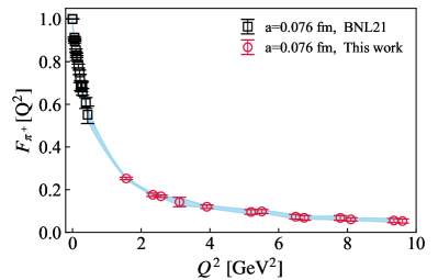
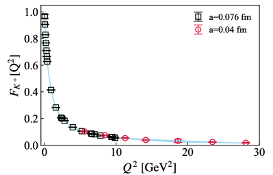
Figure 3: The EMFF of pion (left panel) and kaon (right panel) are shown as a function of $Q^{2}$. For the case of pion, we also include the results from BNL21 [30] using the same lattice setup of the $a$ = 0.076 fm ensemble. For the case of kaon, we have two different ensembles. The bands are from spline interpolation of the first order.

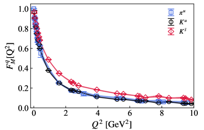
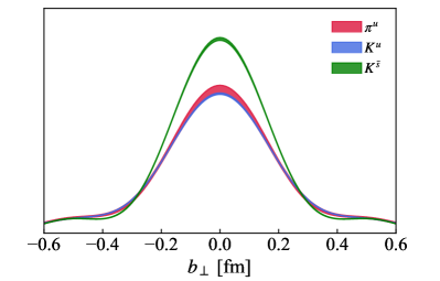
Figure 4: Left: The form factors of valence quarks in pion and kaon are shown as a function of $Q^{2}$. The bands are from spline interpolation of the first order. Right: The flavor distributions of the valence quarks in pion and kaon in the impact-parameter plane are shown as a function of transverse distance $b_{\perp}$.

Appendix B The bare matrix elements of kaon form factors

The analysis of the two-point and three-point function of the pion and kaon, and the extraction of the bare matrix elements follows the strategy laid out in Ref. [30, 41]. Here, we will discuss the case of the kaon as an example. The case of the pion is completely analogous.

B.1 Two-point function analysis

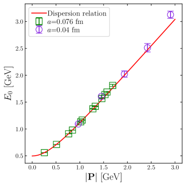
Figure 5: The ground-state energy $E_{0}$ extracted from the two-point functions on the $a$ = 0.076 fm (squared symbols) and 0.04 fm (circled symbols) lattices are shown. The red line is calculated from the dispersion relation $E=\sqrt{m_{K}^{2}+|\textbf{P}|^{2}}$ with $m_{K}$ = 0.497 GeV.

The two-point functions of kaon can be decomposed as

$$\begin{split}C_{\rm 2pt}(\mathbf{P},t_{s})&=\sum_{n=0}^{N_{\rm state}-1}|A_{n}|^{2}(e^{-E_{n}t_{s}}+e^{-E_{n}(aL_{t}-t_{s})}).\end{split}$$ (7)

Here, $E_{n}$ represents the energy levels, $A_{n}=\langle\Omega|K_{S}|n;\mathbf{P}\rangle$ is the kaon overlap amplitude, and $|\Omega\rangle$ denotes the vacuum state. By truncating the spectrum decomposition up to $N$-state, we can extract the first few energy levels and overlap amplitudes by fitting the two-point function data. Here, we choose $N_{\rm state}=2$ to obtain the energy levels and the overlap amplitudes. The results on the ground-state energy of the kaon for different momenta are shown in Fig. 5. As one can see from the figure, the results on the ground-state energy $E_{0}$ as a function of $|\textbf{P}|$ agree very well with the line given by the dispersion relation $\sqrt{m_{K}^{2}+|\textbf{P}|^{2}}$ with $m_{K}$ = 0.497 GeV. We will use the values of $E_{n}$ and $A_{n}$ determined here for the following analysis of three-point functions.

B.2 The ground-state bare matrix elements from three-point function

Similar to the two-point functions, the three-point functions have the spectral decomposition,

$$C_{\rm 3pt}(\mathbf{P}^{f},\mathbf{P}^{i};\tau,t_{s})=\sum_{m,n}A_{m}A_{n}^{*}\langle m;\mathbf{P}^{f}|O_{\Gamma}|n;\mathbf{P}^{i}\rangle e^{-(t_{s}-\tau)E_{m}^{f}}e^{-\tau E_{n}^{i}},$$ (8)

where the overlap amplitudes $A_{n}$ as well the energy levels $E_{n}$ are the same as for the two-point functions, and the ground-state bare matrix element $F^{B}=\langle 0;\mathbf{P}^{f}|O_{\Gamma}|0;\mathbf{P}^{i}\rangle$ is the bare form factor. We construct a ratio defined as

$$R^{fi}(\mathbf{P}^{f},\mathbf{P}^{i};\tau,t_{s})\equiv\frac{2\sqrt{E_{0}^{f}E_{0}^{i}}}{E_{0}^{f}+E_{0}^{i}}\frac{C_{\rm 3pt}(\mathbf{P}^{f},\mathbf{P}^{i};\tau,t_{s})}{C_{\rm 2pt}(\mathbf{P}^{f},t_{s})}\left[\frac{C_{\rm 2pt}(\mathbf{P}^{i},t_{s}-\tau)C_{\rm 2pt}(\mathbf{P}^{f},\tau)C_{\rm 2pt}(\mathbf{P}^{f},t_{s})}{C_{\rm 2pt}(\mathbf{P}^{f},t_{s}-\tau)C_{\rm 2pt}(\mathbf{P}^{i},\tau)C_{\rm 2pt}(\mathbf{P}^{i},t_{s})}\right]^{1/2}$$ (9)

to take advantage of the correlation between two-point and three-point functions. In the $t_{s}\rightarrow\infty$ limit, the ratios give the bare matrix elements of the ground state $R^{fi}(\mathbf{P}^{f},\mathbf{P}^{i},\tau\rightarrow\infty,t_{s}\rightarrow\infty)=F^{B}_{M}(Q^{2})$. Based on the spectral decomposition formula, several methods can be considered to perform the $\tau\rightarrow\infty,t_{s}\rightarrow\infty$ extrapolation of the ratios:

1. Two-state fit. We truncate the spectral decomposition formula of the two-point functions as well as the three-point functions up to two states ($m,n$ can be 0 and 1), insert them into the ratios, and finally get the formula below.

   $$R^{fi}(\mathbf{P}^{f},\mathbf{P}^{i};\tau,t_{s}) =\left[\mathcal{O}_{00}+\frac{|A_{1}^{i}|}{|A_{0}^{i}|}\frac{|A_{1}^{f}|}{|A_{0}^{f}|}\mathcal{O}_{11}e^{(\Delta E^{f}-\Delta E^{i})\tau}e^{-\Delta E^{f}t_{s}}+\frac{|A_{1}^{i}|}{|A_{0}^{i}|}\mathcal{O}_{01}e^{-\Delta E^{i}\tau}+\frac{|A_{1}^{f}|}{|A_{0}^{f}|}\mathcal{O}_{10}e^{-(t_{s}-\tau)\Delta E^{f}}\right]$$ (10)

   $$\quad\times\sqrt{\frac{1+\frac{|A_{1}^{i}|^{2}}{|A_{0}^{i}|^{2}}\frac{|A_{1}^{f}|^{2}}{|A_{0}^{f}|^{2}}e^{-(t_{s}-\tau)\Delta E^{i}}e^{-\Delta E^{f}\tau}+\frac{|A_{1}^{i}|^{2}}{|A_{0}^{i}|^{2}}e^{-(t_{s}-\tau)\Delta E^{i}}+\frac{|A_{1}^{f}|^{2}}{|A_{0}^{f}|^{2}}e^{-\Delta E^{f}\tau}}{1+\frac{|A_{1}^{i}|^{2}}{|A_{0}^{i}|^{2}}\frac{|A_{1}^{f}|^{2}}{|A_{0}^{f}|^{2}}e^{-(t_{s}-\tau)\Delta E^{f}}e^{-\Delta E^{i}\tau}+\frac{|A_{1}^{i}|^{2}}{|A_{0}^{i}|^{2}}e^{-\Delta E^{i}\tau}+\frac{|A_{1}^{f}|^{2}}{|A_{0}^{f}|^{2}}e^{-(t_{s}-\tau)\Delta E^{f}}}}$$

   $$\quad\times\frac{1}{\sqrt{1+\frac{|A_{1}^{i}|^{2}}{|A_{0}^{i}|^{2}}\frac{|A_{1}^{f}|^{2}}{|A_{0}^{f}|^{2}}e^{-(\Delta E^{f}+\Delta E^{i})t_{s}}+\frac{|A_{1}^{i}|^{2}}{|A_{0}^{i}|^{2}}e^{-\Delta E^{i}t_{s}}+\frac{|A_{1}^{f}|^{2}}{|A_{0}^{f}|^{2}}e^{-\Delta E^{f}t_{s}}}}.$$

   In the Breit frame limit, we can use a simplified form for this ratio,

   $$R^{fi}(\mathbf{P}^{f},\mathbf{P}^{i};\tau,t_{s})=\frac{\mathcal{O}_{00}+\frac{|A_{1}|^{2}}{|A_{0}|^{2}}\mathcal{O}_{11}e^{-t_{s}\Delta E}+\frac{|A_{1}|}{|A_{0}|}\mathcal{O}_{01}e^{-\tau\Delta E}+\frac{|A_{1}|}{|A_{0}|}\mathcal{O}_{10}e^{-(t_{s}-\tau)\Delta E}}{1+\frac{|A_{1}|^{2}}{|A_{0}|^{2}}e^{-t_{s}\Delta E}},$$ (11)

   with $\Delta E=E_{1}-E_{0}$ being the energy difference and $\mathcal{O}_{mn}=\langle m;\mathbf{P}^{f}|O_{\Gamma}|n;\mathbf{P}^{i}\rangle$ representing the matrix elements, in which $\mathcal{O}_{00}$ is the bare form factor. We perform the fit using the above expressions by fixing $\Delta E$ as well as $|A_{1}|/|A_{0}|$ to the values obtained from the analysis of the two-point functions, treating $\mathcal{O}_{nm}$ as fit parameters, and skipping $n_{\textup{sk}}$ data points in $\tau$ on the two sides of the source-sink separation to avoid excited-state contamination. In general, this implies a four-parameter fit. In the case of the Breit frame, we have $\mathcal{O}_{01}=\mathcal{O}_{10}$, so we deal with a three-parameter fit. We will refer to this fit method as Fit($n_{\textup{sk}}$). Alternatively, instead of fixing $\Delta E$ and $|A_{1}|/|A_{0}|$, we could impose priors into the $\chi^{2}$ by utilizing their central values and corresponding 1-$\sigma$ errors derived from the two-point functions, and perform a constrained five-parameter fit, with $\mathcal{O}_{00},\mathcal{O}_{01},\mathcal{O}_{11},\Delta E$ and $|A_{1}|/|A_{0}|$ being fit parameters. We refer to this fit method as 2-prior Fit($n_{\textup{sk}}$).

2. Summation method. We construct the sum of the ratios over time insertion $\tau$,

   $$R^{fi}_{\textup{sum}}(t_{s})=\sum_{\tau=n_{\textup{sk}}a}^{t_{s}-n_{\textup{sk}}a}R^{fi}(t_{s},\tau).$$ (12)

   For sufficiently large $t_{s}$, the excited-states contribution is suppressed, and the sum can be approximated by a linear function,

   $$R^{fi}_{\textup{sum}}(t_{s})=nF^{B}+B_{0}+\mathcal{O}(e^{-(E_{1}-E_{0})t_{s}}),\quad n=t_{s}-(2n_{\textup{sk}}-1)a.$$ (13)

   Therefore, we can do a linear fit of data on $R^{fi}_{\textup{sum}}(t_{s})$ to extract the bare form factor, $F^{B}$. One can control the excited-state contamination by choosing different values of $n_{\textup{sk}}$. However, for certain cases when $t_{s}$ is too small, the excited-state contribution cannot be fully ignored. We can include the LO correction term, allowing us to express the ansatz in the Breit frame as

   $$R^{fi}_{\textup{sum}}(t_{s})=nF^{B}+B_{0}+nB_{1}e^{-(E_{1}-E_{0})t_{s}}.$$ (14)

   These two methods will be denoted as Sum(n${}_{\textup{sk}}$) and SumExp($n_{\textup{sk}}$).

3. When the $t_{s}$ is large enough, the excited-states contribution is negligible within the statistic error. In this case, the ratios $R^{fi}(t_{s},\tau)$ would show $t_{s}$- and $\tau$-independent plateaus within the errors. One can simply do a plateau fit to get $F^{B}$. We refer to this method as Plateau($n_{\textup{sk}}$).

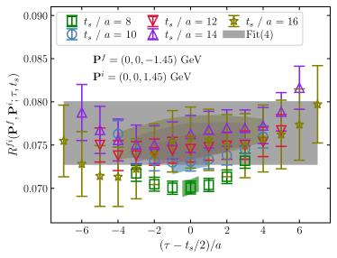
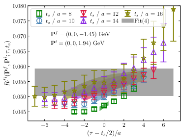
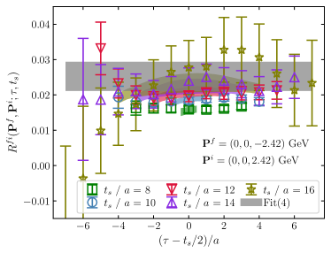
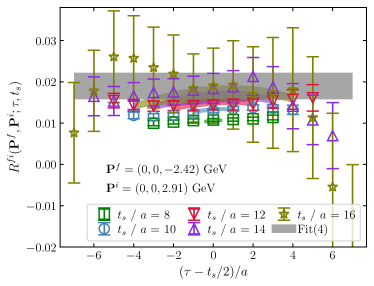
Figure 6: The lattice results of the ratio, $R^{fi}$, and the corresponding two-state Fit($n_{sk}=4$) on $a$ = 0.04 fm lattice are shown. The left panels show examples from the Breit frame, while the right ones are examples from the non-Breit frame. The colored bands present the fit results of the corresponding colored lattice data, while the grey bands show the bare form factor results.

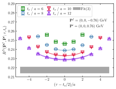
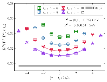
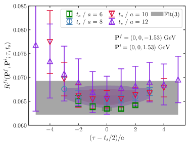
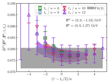
Figure 7: The same as Fig. 6, but for the ratio, $R^{fi}$, on $a$ = 0.076 fm lattice.

In this work, we considered the first two methods. One thing to notice is that $\tau$ has a rather limited range, so the values of $n_{\textup{sk}}$ must be determined appropriately. Since for $a=0.04$ fm ensemble, we have source-sink separations $t_{s}/a=\{8,10,12,14,16\}$, the $\tau$-dependence of the three-point correlators can only be studied for $\tau\lesssim 8a$. Based on our previous experience [30, 41], here we choose $n_{\textup{sk}}\geq 3$. For $a=0.076$ fm ensemble, we have $t_{s}/a=\{6,8,10,12\}$, so the $\tau$-dependence of the three-point function can only be studied for $\tau\lesssim 6a$. Again, based on past experience, we use $n_{\textup{sk}}\geq 2$ in this case. The two-state fits to our lattice data are shown in Fig. 6 and Fig. 7. In Fig. 6, we present the examples of the ratio ($R^{fi}$) for the $a$ = 0.04 fm lattice, with $P_{z}^{f}=-1.45$ GeV varied from $P_{z}^{i}=\{1.45,~{}1.94\}$ GeV in the upper panels, and $P_{z}^{f}=-2.42$ GeV varied from $P_{z}^{i}=\{2.42,~{}2.91\}$ GeV in the lower panels. While Fig. 7 show the cases for the $a$ = 0.076 fm lattice, with $P_{z}^{f}=-0.76$ GeV, varying $P_{z}^{i}=\{0.51,~{}0.76\}$ GeV in the upper panels, and $P_{z}^{f}=-1.53$ GeV, varying $P_{z}^{i}=\{1.27,~{}1.53\}$ GeV in the lower panels. In each panel, the colored bands represent the fit results using the two-state Fit($n_{\rm sk}$) method, while the grey bands denote the extrapolated bare form factor results, $F^{B}$. The color coding of the bands corresponds to the color coding of the lattice data for different source-sink separations.

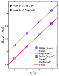
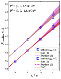
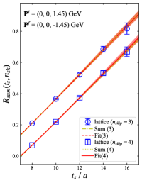
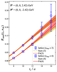
Figure 8: The summation of ratios $R^{fi}_{\textup{sum}}(t_{s})$ for $a$ = 0.076 fm (left two panels) and $a$ = 0.04 fm lattice (right two panels) are shown. The curves are reconstructed from the summation fit as well as the two-state fit results.

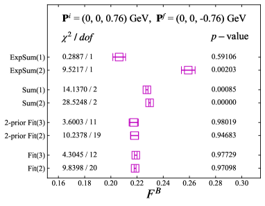
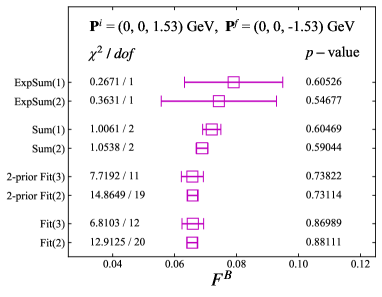
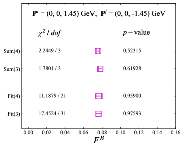
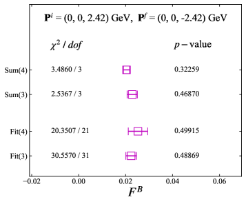
Figure 9: The results and fit quality from the summation fit and two-state fit with different numbers of skipped time insertion $n_{sk}$ are shown for comparison. Upper: $a$ = 0.076 fm lattice, lower: $a$ = 0.04 fm lattice.

In Fig. 8, we show the lattice results for $R^{fi}_{\textup{sum}}(t_{s})$ together with the correspondings fit results from Sum($n_{\textup{sk}}$), ExpSum($n_{\textup{sk}}$), and Fit($n_{\textup{sk}}$) for both $a=0.04$ fm lattice (left two panels) and $a=0.076$ fm lattice (right two panels). Furthermore, the values of the bare form factor obtained using these fit methods are summarized in Fig. 9. In this figure, we also show the corresponding $\chi^{2}/dof$ and $p$-value for each method. As one can see, the two-state fits always give $\chi^{2}/dof\lesssim$ 1 and consistent results for different choices of $n_{\textup{sk}}$, suggesting this method is robust for the data under consideration. For the $a$ = 0.076 fm ensemble and small momenta cases, the summation fits, Sum($n_{\textup{sk}}$), have large values of $\chi^{2}/dof$. This is because the statistical errors in these cases are small, and excited-state contamination cannot be neglected. In this situation, it is necessary to introduce the excited-state corrections to the summation method, namely ExpSum($n_{\textup{sk}}$). The results from ExpSum($n_{\textup{sk}}$) show reasonable $\chi^{2}/dof$, but the errors become large since it is difficult to fit three parameters using only a few data points. On the other hand, the results from ExpSum($n_{\textup{sk}}$) are consistent with the two-state fit within errors. For the $a$ = 0.04 fm lattice with larger momenta cases, the excited-state contamination is small compared to the statistical errors, so that the results from Sum($n_{\textup{sk}}$) method agree with the corresponding results from the two-state fit. Moreover, a comparison of the Breit frame results between the normal Fit and prior Fit methods in the upper panels of Fig. 9 reveals that they are in good agreement with the 1-$\sigma$ error. However, the error magnitude of the prior method can be affected by many factors, like the range of the priors and the statistics, which will sometimes lead to an unreliable error range. Therefore, for the $a=0.076$ fm lattice, we choose the 2-prior Fit(3) results for the Breit frame case and the general Fit(3) results for the non-Breit frame case. For the $a=0.04$ fm lattice, we select the results from general Fit(4) for all cases.