Abstract

Scenarios seeking to address the issue of electroweak symmetry breaking often have heavy colored gauge bosons coupling preferentially to the top quark. Considering the bulk Randall-Sundrum as a typical example, we consider the prospects of the first Kaluza-Klein mode ($G^{(1)}$) of the gluon being produced at the LHC in association with a $t\overline{t}$ pair. The enhanced coupling not only dictates that the dominant decay mode would be to a $t\overline{t}$ pair, but also to a very large $G^{(1)}$ width, necessitating the use of a renormalised $G^{(1)}$ propagator. This, alongwith the presence of large backgrounds (specially $t\overline{t}jj$), renders a conventional cut-based analysis ineffective, yielding only marginal significances of only around 2$\sigma$. The use of Machine Learning (ML) techniques alleviates this problem to a great extent. In particular, the use of Artificial Neural Networks helps us identify the most discriminating observables, thereby allowing a significance in excess of 4$\sigma$ for $G^{(1)}$ masses of $\sim$ 4 TeV.

1 Introduction

Despite its unprecedented success in describing experimental results, the Standard Model (SM) is expected to be only an effective theory on account of its failure to address a host of issues. Hence, despite the lack of any direct evidence of new physics at the LHC, the search goes on. Of particular interest is unravelling the nature of electroweak symmetry breaking (EWSB), which continues to be be little-understood despite the discovery of a Higgs scalar. With the top quark being the heaviest particle within the SM, with a mass close to the EWSB scale, it is expected to provide a sensitive probe for not only the symmetry breaking sector [1, 2], but also to a variety of possible scenarios going beyond the SM. This is understandably true for models wherein the new physics sector has enhanced couplings to the top quark, examples being topcolor [3, 2], topcolor assisted technicolor [4] or certain models defined on a warped 5-dimensional space. More interestingly, even in the absence of such an enhancement (such as for generic coloron models [5, 6] or axigluons [7, 8]), the unique signal profiles that, say, a $t\overline{t}$ final state provides, as also the smaller (as compared to a dijet final state) SM background that this channel is associated with, render (multi-)top-quark production very attractive arenae to probe such theories.

The models mentioned above typically incorporate an extended color symmetry, typically of the form $SU(3)_{I}\otimes SU(3)_{II}\to SU(3)_{c}$ with the breaking occurring at a high enough scale. They differ from each other in both the details of how $SU(3)_{c}$ is embedded in the larger group (including whether the said group encompasses a chiral symmetry) as also in the representations (and, hence, the couplings) of the SM fermions. Quite understandably, the symmetry can be enhanced almost arbitrarily with extra factors of $SU(3)$’s associated with different couplings. Furthermore, differing symmetry breaking chains and/or embeddings of fermions would result in different relations between the gauge couplings. In other words, these models could be envisaged as different low-energy realizations (or deconstructions) of a deeper theory.

The warped extra dimension framework due to Randall and Sundrum (RS) [9], defined on a modest-sized (in the fifth direction) slice of AdS₅, presents one such scenario. Originally motivated as a solution to the Planck scale–weak scale hierarchy problem within the SM, this was constructed by localizing the usual (four-dimensional and massless) graviton near an end-of-the-world (UV) brane attributed with a Planckian fundamental scale, whereas the SM sector (including the Higgs) was localized on the opposite (IR) brane whence the scale is protected by the warping-down of the fundamental scale. However, it was soon realized that on considering the $5D$ effective field theory, higher-dimensional operators are suppressed only by the warped-down scale ($\sim$ a few TeVs), leading to untenably large contributions to flavour-changing neutral current (FCNC) processes as well as electroweak precision observables and/or proton decay.

Going beyond the original motivation and extending [10, 11, 12] the gauge and fermion fields into the bulk (of the warped extra dimension) as well removes some of these constraints. Compactifying the fifth dimension now results in towers of fermions and gauge bosons, with the last-mentioned being the analogues of the heavy gauge bosons in the extended color symmetry models. The profiles (wavefunctions) of these Kaluza-Klein excitations (bosonic as well as fermionic) would depend on the details of the warping (such as whether it is engendered by a bulk cosmological constant alone or if, say, a nontrivial dilaton field is involved as well) as well as the bulk masses of the fields (other than the gauge fields). Localizing the first two generation fermions near the Planck brane automatically suppresses the FCNC’s as well as contributions to electroweak precision test observables  [12, 13] on account of the effective cutoff being nearly Planckian in the vicinity. Furthermore, with the overlap of the wavefunctions playing a crucial role in the determination of the effective Yukawa couplings, a solution to the SM flavour problem is now obtainable with only a very moderate hierarchy in the bulk fermion masses. Such welcome features has spawned an abiding interest in such Bulk RS models [10, 14, 15, 16, 17, 18, 19, 20, 21].

In the majority of such models, the heavy colored gauge bosons have enhanced couplings with at least some of the SM fermions, most often the top-quark. While, in the generic coloron or axigluon models, this comes about in the quest of a dynamical origin to EWSB, for the RS gluons (depicted by $G^{(1)}$) this results from the aforementioned nontrivial profiles in the bulk. Consequently, $t\overline{t}$ production (whether at the Tevatron or the LHC) has long been a favoured channel to probe such models [22, 23, 24, 25]. However, such analyses need to be approached with care. Owing to the aforementioned coupling enhancements, such a gluon has a naturally large width and the narrow width approximation is often not valid [25, 26, 27]. And, away from the peak, the signal often tends to get submerged in the extremely large QCD rates. The channel also has a subdominant behaviour because of being initiated by a quark-antiquark fusion (dominated by light quarks), where the relatively small coupling of $G^{(1)}$ with the light quarks result in very small production cross-section compared to the $t\overline{t}$ SM background. Consequently, alternative channels need to be probed and, in this paper, we consider the four-top ($t\overline{t}t\overline{t}$) signal. While this channel has been considered in the past [28, 29] for various beyond-the-SM scenarios, the large width presents its own challenges (both theoretical and experimental), and we include the effects in self-consistently. The cross-section for this channel is also very small, but we can leverage on the fact that the two top quarks enamating from the heavy $G^{(1)}$ will be highly boosted, giving us a way to discriminate over the towering SM backgrounds. This, however, is not a simple task. As we shall see, simple cut-based techniques cannot meaningfully discriminate the signal, with the main culprit being the $t\overline{t}jj$ ($j$ being light jets) background. This compels us to look at machine learning methods, specifically Artificial Neural Networks (ANNs) for better discriminating power, and this we would discuss in great detail.

The rest of this article is constructed as follows. In the next section, we begin by outlining the class of scenarios that incorporate gluon resonances, culminating with a specific choice that we would concentrate on as a template model. Typically, such resonances tend to be rather broad, necessitating a proper treatment of the propagator, and this we review in Section 3. In the subsequent section, we delineate the signal characteristics at the Large Hadron Collider, and discuss the various sources of backgrounds, reducible and irreducible. In Section 5, we discuss in detail the signal and the (much larger) background profiles and attempt a cut-based analysis, demonstraing how the significance of a signal-excess could be established. As a complementary approach, we examine, in Section 6, the efficacy of employing machine learning techniques in this context. We establish that the use of Artifical Neural Networks can significantly enhance the reach of the LHC. Finally, we conclude in Section 7.

2 Model

The model of our interest is defined on a slice of AdS₅ described by the metric

$$ds^{2}=e^{-2A(y)}\eta_{\mu\nu}dx^{\mu}dx^{\nu}-dy^{2}$$

with $\eta_{\mu\nu}={\rm diag}(1,-1,-1,-1)$ and the fifth dimension being a segment of real line, namely $y\in[0,\pi r_{c}]$. The background gravity is assumed to be defined by the Einstein-Hilbert action in five dimensions (with a characteristic scale $M_{5}$ not too different from $M_{\rm Pl}$) augmented by a substantial negative cosmological constant ($-\Lambda$), that is not so large as to invalidate a semiclassical treatment. This leads to

$$A(y)=-k|y|\ ,\qquad\quad k=\sqrt{\frac{\Lambda}{24M_{5}^{3}}}\ ,$$

and for $kr_{c}\sim 12$ (easily achieved if $r_{c}$ is somewhat larger than $M_{5}^{-1}$ as is also required for a semiclassical treatment to be valid), the warping between the scales induced on the two end-of-the-world (i.e., at $y=0$ and $y=\pi r_{c}$) 3-branes mirrors that between $M_{\rm Pl}$ and the electroweak scale [9]. For the system to be consistent (i.e., for the Israel junction conditions to be satisfied), the two branes need to be associated with equal and opposite brane tensions related, in turn, to $\Lambda$.

The resolution of the hierarchy obviously requires a specific value for the distance modulus $r_{c}$. This can be addressed by invoking a bulk-propagating scalar field $\phi$ ascribed with a potential $V(\phi)$. A self-consistent solution of such a graviton-radion system automatically generates a stabilized solution for $r_{c}$. Both the graviton and the radion can be expanded in terms of the respective Kaluza-Klein modes. The lowest (massless) graviton mode has a profile peaked near the (UV) brane located at $y=0$, and naturally has only a highly suppressed coupling with the SM fields which are localized on the IR brane (at $y=r_{c}$). And while the higher modes have relatively unsuppressed couplings (of the order of the electroweak gauge couplings), the masses of these resonances (in the TeVs) render their effects small.

While the aforementioned (RS) model provides a natural solution for the electroweak-Planck scale hierarchy, it does not address another vexing issue within the SM, namely the flavour problem. Not only is the hierarchy between the fermion masses unexplained, the low effective scale ($\sim$ TeV on account of the warping-down) of new physics implies that higher-dimensional operators do not suffer large suppressions and, thus, unwanted features such as flavour-changing neutral current (FCNC) processes or proton-decay stand to have uncomfortably large amplitudes.

An attractive solution to this problem appears if we allow the SM fields to propagate in the bulk [10, 14, 11, 12]. The SM fermion is now identified with the chiral zero-mode of the $5D$ fields, with the profile (localization) along the extra dimension being determined by its $5D$ mass parameter. Very moderate hierarchies in these parameters change the profiles considerably. Understandably, localizing the fermion fields towards the UV (IR) branes implies light (heavy) masses for the low-lying modes as the Higgs is resolutely localized on (or close to) the IR brane. This automatically ensures that the FCNCs from higher-dimensional operators are suppressed by effective cut-off scales (typically, $\gg$ TeV) at the location of these fermions [12, 13]. Quite analogously, contributions to the electroweak precision observables are suppressed too.

The propagation of the fermions into the bulk, of course, necessitates that the gauge bosons must do so too. Once again, the lowest-lying mode is massless and has a trivial profile. The higher KK-modes, though, are massive and have nontrivial profiles. It is the last mentioned property that, coupled with the non-identical profiles of the fermions, leads to unequal couplings of the SM fermions (i.e., the respective lowest-lying modes) to the higher KK-gauge bosons and, thereby results in FCNCs. However, the very structure of the theory ensures that the non-universal part of these couplings are proportional to the SM Yukawa couplings [12, 13]. With the new degrees of freedom being heavy and their couplings to fermions of the first two generations being small (a consequence of the respective localizations), there exists an approximate symmetry structure that suppresses the FCNCs (at least amongst the lowest-lying modes) adequately [30]. And while additional contributions to the electroweak precision variables (primarily, the $S$ and $T$ parameters) emerge from the gauge KK modes, the ensuing constraints can be satisfied for a KK mass scale as low as $\sim 3$ TeV once a custodial isospin symmetry is imposed [31].

We are now in a position to consider the interactions of the gluons $G_{\mu}^{(n)a}$ of the $n$-th KK level with the SM fermions. The interaction Lagrangian of interest can be expressed as

$$\mathcal{L}^{(n)}_{RS}\, = \,-\,\frac{1}{4}G^{(n)a}_{\mu\nu}\,G^{(n)a\,\mu\nu}-m_{n}^{2}\,G^{(n)a}_{\mu}\,G^{(n)a\,\mu}+\sum_{q}\sum_{j=L,R}g^{(n)}_{q_{j}}\overline{q_{j}}\,\gamma^{\mu}\,T^{a}\,q_{j}\,\,G^{(n)a}_{\mu}$$ (1)

where $q$ denotes the flavour and $g^{(n)}_{q_{j}}$ the corresponding coupling to a quark of flavour $q$ and chirality $j$. In particular, we would be interested in the top/bottom sector. Clearly, if we seek to localize both $t_{L,R}$ near the UV-brane, the ensuing top Yukawa coupling would be too small. On the other hand, localizing $(t,b)_{L}$ close to the IR-brane leads to it having a relatively large coupling to the $Z_{\mu}^{(n)}$ (for $n>0$). The mixing of the latter with the ordinary $Z$ (i.e., $Z_{\mu}^{(0)}$), in turn, results in a non-universal shift in the latter’s coupling to the $(t,b)_{L}$ [31]. In particular,

$$\delta g^{(Z)}_{b_{L}}\sim\sqrt{\log\frac{M_{\rm Pl}}{1\mbox{ TeV }}}g^{Z^{(n)}}_{b_{L}}\frac{m^{2}_{Z}}{M_{n}^{2}}$$

where $g^{Z^{(n)}}_{b_{L}}$ is the (non-universal) coupling of the $Z^{(n)}$.

With experimental constraints (emanating largely from electroweak precision tests) stipulating that $\delta g^{(Z)}_{b_{L}}/g^{(Z)}\raisebox{-1.72218pt}{\hbox to0.0pt{$\sim$\hss}}\raisebox{1.72218pt}{$<$}1.4\%$[32], it is evident that if the mass of the first KK-resonance $\simeq$ a few TeV, there is a seeming tension between this constraint and the need to have a large top mass. This can, however, be relaxed, even for dimensionless $5D$ Yukawa couplings consistent with perturbativity. An example is afforded by quasi-localizing the $(t,b)_{L}$ doublet near the IR-brane (so that the shift $\delta g^{(Z)}_{b_{L}}$ remains consistent with the data) and simultaneously localizing $t_{R}$ very close to the IR-brane so as to enable a large top quark mass. Note that the resulting coupling of the $b_{L}$ to the gauge KK modes (including gluon) is comparable to the SM couplings and, in being dictated by the large top mass, is, thus, still larger than what is expected on the basis of $m_{b}$ alone. Consequently, even with such choices, the KK scale is required to be rather high, namely, $\sim 5$ TeV.

As can be imagined, the constraints do depend on the symmetries imposed and the assignments, e.g. the representation of the heavy quarks under the custodial isospin symmetry [33]. Indeed, for certain choices of profiles for $t_{R}$ and $(t,b)_{L}$, the KK scale can be as low as $\sim 3$ TeV [34]. In the rest of this paper, we consider the assignments of Ref. [23], wherein the couplings of $G^{(1)}$ to a light quark (including the $b_{R}$) pair are suppressed by a constant $\xi$ with respect to the standard QCD coupling. As for its coupling to a gluon pair, it is even further suppressed (vanishing at the leading order) owing to the orthogonality of profiles. In other words, the $G^{(1)}$ is “proton-phobic”. The coupling to $(t_{L},b_{L})$ is largely unchanged. As for the $t_{R}$, which is localized very close to the IR brane (or, in the dual picture, is a composite), its coupling to the $G^{(1)}$ is enhanced by $\xi$. In other words, and using an obvious notation,

$$\begin{array}[]{rclcrcl}g_{qqG^{(1)}}&\simeq&\xi^{-1}g_{s}&&g_{ggG^{(1)}}&\approx&{\Large 0}\\[8.61108pt] g_{Q_{3}Q_{3}G^{(1)}}&\approx&g_{s}&&g_{t_{R}t_{R}G^{(1)}}&\approx&\xi g_{s}\ ,\end{array}$$ (2)

where $g_{s}$ is the usual strong coupling, $Q_{3}\equiv(t,b)_{L}$ and $q$ comprises all of $u_{L,R},d_{L,R},s_{L,R},c_{L,R}$ as well as $b_{R}$. For most of our numerical work, we would use $\xi=5$ (as advocated in Ref.[23]) as our benchmark value.

3 Renormalised KK gluon propagator

While it is commonplace to consider the Breit-Wigner form as the propagator for a massive and unstable particle, this is straightforward only in the case of a very narrow width. Else, care needs to be taken to preserve gauge invariance. In the present case, the enhanced coupling of the KK gluon to the right-handed top quarks leads to a significantly large decay width of the KK gluon as given by

$$\begin{array}[]{rcl}\Gamma&=&\sum_{q}\Gamma(G^{(1)}\to q\overline{q})\,\ =\,\ \dfrac{M_{G^{(1)}}}{48\pi}\sum_{q}\sqrt{1-\dfrac{4m_{q}^{2}}{M_{G^{(1)}}}}\left[(g_{q_{L}}^{2}+g_{q_{R}}^{2})\left(1-\dfrac{m_{q}^{2}}{M_{G^{(1)}}}\right)+6g_{q_{L}}g_{q_{R}}\dfrac{m_{q}^{2}}{M_{G^{(1)}}}\right]\ .\end{array}$$ (3)

where the couplings $g_{q_{L}}$ and $g_{q_{R}}$ are as in Eq. 2. For a sufficiently heavy $G^{(1)}$ and a large enough value of $\xi$ (as we are interested in), we have $\Gamma\approx\xi^{2}\alpha_{s}M_{G^{(1)}}/12$, which translates to several hundreds of GeVs. Such a broad resonance has to be dealt with carefully, and gauge invariance ensured [27].

Reminding ourselves that the Breit-Wigner form originated from the imaginary part of the self-energy correction (courtesy the optical theorem and the Cutkosky rules), we begin by listing the same for the $G^{(1)}$. To the one-loop order, this is straightforward and, for a $G^{(1)}$ of momentum $k$, is given by

$$i\Pi^{ab}_{\mu\nu}(k^{2})=i\delta^{ab}\left[g_{\mu\nu}k^{2}\Pi(k^{2})-k_{\mu}k_{\nu}\Delta_{\Pi}(k^{2})\right]\ ,$$ (4)

with $\Pi(k^{2})=\overline{\Pi}(k^{2})+\delta M^{2}/k^{2}$ and

$$\begin{array}[]{rcl}\overline{\Pi}(k^{2})&=&\Delta_{\Pi}(k^{2})+\dfrac{1}{16\pi^{2}}\sum_{q}(g_{q_{L}}-g_{q_{R}})^{2}\dfrac{m_{q}^{2}}{k^{2}}\left[2+\mathcal{F}_{q}(k^{2})\right]\ ,\\[12.91663pt] \Delta_{\Pi}(k^{2})&=&\dfrac{-1}{48\pi^{2}}\sum_{q}(g_{q_{L}}^{2}+g_{q_{R}}^{2})\left[\dfrac{2}{\varepsilon}-\gamma_{E}+\ln\dfrac{4\pi\mu^{2}}{m_{q}^{2}}+\dfrac{5}{3}\left(1+\dfrac{12m_{q}^{2}}{5k^{2}}\right)+\left(1+\dfrac{2m_{q}^{2}}{k^{2}}\right)\mathcal{F}_{q}(k^{2})\right]\ ,\\[12.91663pt] \end{array}$$ (5)

Here $\varepsilon$ is the regulator of the ultraviolet divergence, $\gamma_{E}$ is the Euler-Mascheroni constant, $\mu$ is the arbitrary scale which appears in dimensional regularization, and $m_{q}$ is the quark mass. The loop integrals $\mathcal{F}_{q}(k^{2})$ are functions of the familiar kinematic variable $\beta_{q,k}\equiv(1-4m_{q}^{2}/k^{2})$, namely

$$\mathcal{F}_{q}(k^{2})=\left\{\begin{array}[]{ll}\sqrt{\beta_{q,k}}\left(\ln{\dfrac{1-\sqrt{\beta_{q,k}}}{1+\sqrt{\beta_{q,k}}}}+i\pi\right)&\quad\mbox{for}\quad k^{2}\geq 4m_{q}^{2}\\[12.91663pt] -2\sqrt{-\beta_{q,k}}\;\arctan{\dfrac{1}{\sqrt{-\beta_{q,k}}}}&\quad\mbox{for}\quad k^{2}<4m_{q}^{2}\ .\end{array}\right.$$ (6)

Defining the subtraction scheme so that the mass is given by

$$\delta M^{2}=\dfrac{1}{16\pi^{2}}\sum_{q}(g_{q_{L}}-g_{q_{R}})^{2}m_{q}^{2}\left(\dfrac{2}{\varepsilon}-\gamma_{E}+\ln\dfrac{4\pi\mu^{2}}{m_{q}^{2}}\right)\ ,$$ (7)

the corrected KK-gluon propagator, to one loop, after summing all the one-particle-reducible diagrams is

$$\begin{array}[]{rcl}iG_{\mu\nu}^{ab}&=&iG_{\mu\nu}^{(0)ab}+iG_{\mu\alpha}^{(0)ac}i\Pi^{\alpha\beta}_{cd}(q^{2})iG_{\beta\nu}^{(0)db}+\cdots\\[8.61108pt] &=&i\delta^{ab}\left[\dfrac{-g_{\mu\nu}+\frac{k_{\mu}k_{\nu}}{k^{2}}}{k^{2}-M_{0}^{2}}\left(1+\dfrac{k^{2}\Pi(k^{2})}{k^{2}-M_{0}^{2}}\right)+\dfrac{k_{\mu}k_{\nu}}{k^{2}}\dfrac{1}{M_{0}^{2}}\ \mbox{terms}+\cdots\right]\\[17.22217pt] &=&i\delta^{ab}\left(\dfrac{-g_{\mu\nu}+\frac{k_{\mu}k_{\nu}}{k^{2}}}{k^{2}-M_{0}^{2}-k^{2}\Pi(k^{2})}+\dfrac{k_{\mu}k_{\nu}}{k^{2}}\dfrac{1}{M_{0}^{2}}\ \mbox{terms}\right)\ ,\end{array}$$ (8)

where $iG_{\mu\nu}^{(0)ab}=i\delta^{ab}\frac{-g_{\mu\nu}+\frac{k_{\mu}k_{\nu}}{M_{0}^{2}}}{k^{2}-M_{0}^{2}}$ is the propagator at zeroth order in the unitary gauge and $M_{0}$ the KK-gluon bare mass. Contributions from the $k_{\mu}k_{\nu}$ terms are proportional to the masses of the external particles ($m_{q}^{2}/M_{G^{(1)}}^{2}$) and, hence, are small indeed (even for the top-current). This, then, provides the proper expression for the propagator to this order.

4 Collider signatures

With the $gG^{(1)}G^{(1)}$ coupling being unsuppressed (a consequence of gauge invariance), the naive expectation would be that QCD-driven pair production would constitute the dominant mode at the LHC. However, the very large mass of the $G^{(1)}$ leads to a kinematic suppression. Similarly the rather suppressed $ggG^{(1)}$ and $q\overline{q}G^{(1)}$ (for light quarks) couplings come in the way of resonant single production cross section being substantial. Although the last mode has been examined in the literature [22, 23, 24, 25], we eschew it altogether.

4.1 4-top Signal and 4-top SM background

Instead, the process of interest to us is $G^{(1)}$ production in association with a $t\overline{t}$ pair, where we take advantage of the rather enhanced $t\overline{t}G^{(1)}$ coupling. The very same fact (of enhanced coupling) also stipulates that any $G^{(1)}$ thus produced must decay primarily into a $t\overline{t}$ pair. It must be borne in mind that the large mass of the $G^{(1)}$ and the large $t\overline{t}G^{(1)}$ coupling, together, leads to a large width for the KK-gluon (as discussed in the preceding section). These twin facts (large mass and large width) together imply that a very substantial part of the signal would emanate from an off-shell $G^{(1)}$. In other words, the processes of interest are

$$gg,q\overline{q}\to t\overline{t}G^{(1)(*)}\to t\overline{t}t\overline{t}$$ (9)

where the gluon-initiated subprocess, naturally, dominates. Clearly the process, as seen in terms of the intial and final states, also occurs purely within the SM, and given the fact that the signal events are not associated with a narrow resonance, the interference between the SM and NP amplitudes is not negligible and may significantly affect the event profile.

The 4-top final state within the SM has been well-studied and, at the next-to-leading order [36], has a cross-section of about 15.7 fb. The signal cross section presents a more complicated picture, though. Had it been dominated by the production (and subsequent decay) of a narrow $G^{(1)}$ resonance, clearly the cross-section would have scaled largely as $\left[g_{t_{R}}^{(1)}\right]^{2}$. Indeed, even accounting for the large width of the KK-gluon, the total amplitude of the $G^{(1)}$-mediated diagram would still be nearly proportional to $g_{t_{R}}^{(1)}$. However, the considerable interference between the NP and the SM amplitudes means that the size of the signal, defined as

$$\sigma_{\rm Signal}\equiv\sigma_{SM+NP}(4t)-\sigma_{SM}(4t)$$ (10)

is no longer a simple function of $g_{t_{R}}^{(1)}$. This is exhibited in the behaviour of the total cross sections as displayed in Fig.1.

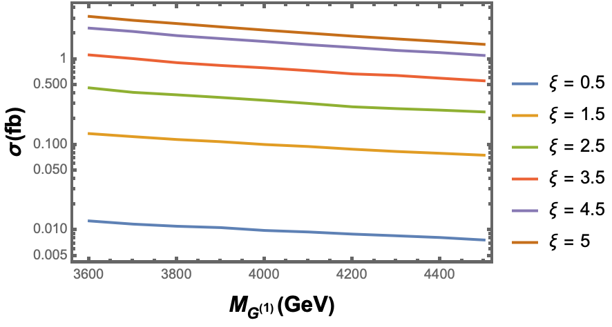
Figure 1: The total signal cross section (as defined in Eq. 10) as a function of the the KK-gluon mass for various values of $\xi$.

Furthermore, the considerable similarity between the signal and the irreducible background (defined as $\sigma_{SM}(4t)$) implies that the separation between the two in the data would not be straightforward. This is particularly worrisome as, for allowed values of the couplings and masses, $\sigma_{\rm Signal}$ tends to be smaller than $\sigma_{\rm SM}(4t)$ and similar signal profiles would render difficult the task of separating the signal from the background. On the other hand, this very similarity allows us to use the NLO $K$-factor, as derived [36] within the SM, to be used for the entire sample, without risking large inaccuracies. It might be argued here that the large mass of the $G^{(1)}$ would imply that the $t\overline{t}$ pair coming off it would be highly boosted and, hence, render the topologies markedly different. However, while the first part of the argument is certainly true (and would be used to our advantage), note that the large width of the KK-gluon, convoluted with the fact that the parton-fluxes fall off rapidly at large subprocess center-of-mass energies, results in a considerable similarity between the events so as to render this approximation (of similar $K$-factors) to be quite admissible.

To understand the possible event profiles, it is necessary to consider the decays of the particles produced in the primary process. As is well-known, a top quark decays overwhelmingly into a $b$-quark and a $W$-boson with the latter, in turn, decaying promptly into a pair of light quarks or to a lepton-neutrino pair. In other words, the four-top state would almost always have four $b$-jets; this apart, it can be classified into five categories [37], namely a completely hadronic (jets) state, or states with hard and isolated charged leptons (the count varying from one to four) accompanied by missing transverse momenta. (In listing this, we are neglecting the further decay of the $b$-hadrons.) In the context of the signal-like events, the large mass of the $G^{(1)}$ means that the $t\overline{t}$ pair from the $G^{(1)}$ leg would tend to be highly boosted. Consequently, their decay products would tend to be collimated and lead to “fatjets”. In anticipation of this, we demand that there be two fatjets in the event, with each having a jet mass around $m_{t}$. We still need to decide how the other two tops decay. As we would see in the subsequent sections, opting for the hadronic decay of one top and leptonic decay of the other would give us the largest signal significance.

4.2 Other major Backgrounds

Several other disparate processes may potentially contribute to the background, depending on how the signal profile is defined. For example, if all the tops were to decay hadronically, then, QCD multijet production, with a cross section that is several orders of magnitude larger, could, presumably, overwhelm the signal. It is here that the fact that the signal events would, typically, contain two fatjets, each reconstructing to the top (even if with a non-negligible experimental tolerance) plays a crucial role. This requirement, immediately, ensures that only those SM events that contain at least two tops would contribute majorly to the background. Apart from the SM four-top events, these include:

• $t\overline{t}jj$ : With $t\overline{t}$ production cross section being very large indeed, one would assume that this particular cross section would also be very large, if only on account of initial-state and final-state radiation. The size of the cross section, of course, depends on the demands made on the transverse momenta of the jets as well as their separation from the beam directions and each other. Canonical basic requirements are that the putative jets be central (with rapidity obeying $|\eta|\leq 3$), have $p_{T}(j)\geq 20$ GeV after ensuring that they are reconstructible as jets and are angular-separated by $\Delta R_{jj}>0.4$. Ref. [38] estimates a cross section ($\sim\,$ 106 pb) for 14 TeV at NLO with the corresponding K-factor 0.89.

  Although only a small fraction of the tops in such a sample would be boosted, yet a few of those undergoing three-pronged hadronic decays would still be reconstructed as a fatjet, especially if a large radius $R$ is used for the jet recontruction algorithm. Consequently, the much larger production cross section renders this a major background. One way to reduce this background is to demand for two independent $b$-tagged jets accompanying the top fatjets. For a genuine 4-top event, such $b$’s would emerge from the decays of the less energetic tops, and the signal would not be impacted by this cut. The $t\overline{t}jj$ background would, however, reduce drastically. Additional backgrounds accrue from events wherein a charm quark ($c$) is sometimes mistagged as a $b$ jet. Such mistagging, though, has only a $10\%$ probability, whereas the probability of other quarks and gluons being mistagged as a $b$ jet is less than $0.1\%$. An useful tool to further suppress all such background is to demand one or more isolated hard leptons (which, for the signal events, can emanate from the leptonic decay of the $W$).

• $t\overline{t}b\overline{b}$ : Compared to the preceding case ($t\overline{t}jj$), it has a much smaller cross-section ($\approx$ 2.64 pb) for 14 TeV at NLO with the corresponding K-factor 1.77 [39, 40]). Once again, demanding two top fatjets would reduce this background substantially. On the other hand, it would not be further suppressed on demanding two $b$-tagged jets. However, demanding one or more leptons as argued for in the previous case would make this background almost negligible.

• $t\overline{t}W$ : This has a comparatively smaller cross-section of $0.577$ pb for 13 TeV at NLO with the corresponding K-factor 1.58  [36], and is expected to reduce drastically once we demand two top fatjets and two $b$-tagged jets.

5 Signal and Background simulations

As the discussion in the preceding section shows, the case of both of the two softer top quarks decaying fully hadronically would be associated with a large SM background (primarily from $t\overline{t}jj$ production). In view of this, we stipulate that the signal events must have at least one of the tops decaying semileptonically (in particular, to a state containing either an electron or a muon). The somewhat smaller branching fraction ($\approx 8/27$ as opposed to $\approx 4/9$ for the fully hadronic mode) is more than compensated for by the background reducing manifold. Thus, we would demand that the final state contains two fatjets (with masses close to $m_{t}$), additional (at least four more) jets, a hard isolated light lepton ($e^{\pm}$ or $\mu^{\pm}$) and some missing tranverse momentum.

5.1 Details of Simulation

Implementing the model in FeynRules [41, 42], we generate signal and background events using MadGraph5_amc@nlo [43] augmented by the implementation of the renormalised RS gluon propagator as discussed in Sec 3. To this end, we use the default dynamic scale ($\mu$) choice in MadGraph5_amc@nlo (which equals the central transverse mass ($m_{T}$) given by $m_{T}$ = $\sqrt{m^{2}+p^{2}_{T}}$ , $m$ being the mass of the top, and $p_{T}$ the transverse momentum after the $k_{T}$ clustering on LHE-level final states ) and the NNPDF parton distributions [44]. Interfacing with Pythia8 [45] for parton showering and fragmentation, the events are then passed through Delphes-3 [46], in order to implement detector effects and apply reconstruction algorithms. The multiple jets in the event (including the two boosted jets from the $G^{(1)}$ leg) are reconstructed and identified with the FastJet module using the anti-$k_{T}$ algorithm. To start with, we only demand $p_{T}\geq 20$ GeV and $|\eta|\leq 2.4$ for all jets in the event. As for the radius parameter $R$ used in reconstructing a fatjet, we investigated the performance for different values and found $R\approx 0.5$ to be an optimum choice. Too small a value of $R$ would result in very few events being reconstructed as containing fatjets, while too large a value would result in virtually all events being reconstructed as having a fatjet. Given the mass of the $G^{(1)}$ being explored, it can actually be estimated that $R=0.5$ would be optimal in capturing both the (boosted) tops from the $G^{(1)}$ being reconstructed as a fatjet, while simultaneously rejecting the less energetic background tops owing to their failure to reconstruct within a similar cone. For other parameters of the jet-substructure observables, we use the default values of the Delphes card from Delphes-3 [46]. For lepton isolation too, we use the default values, which requires that there be no other charged particles with $p_{T}>0.5$ GeV within a cone of $\Delta R<0.5$.

In the rest of this section, as also in the next, we include all the major backgrounds mentioned in the preceding section as also the subdominant ones (without showing the latter in the plots). As for the signal, this is defined as the $\overline{t}t\overline{t}t$ sample, where the SM contribution has been exactly subtracted out (see Eq.10). In other words, it is defined as the sum of the contributions of the pure $G^{(1)}$ piece as well as that due to the interference of the $G^{(1)}$-mediated amplitude with the SM one.

5.2 Signal-Background profiles

5.2.1 Dominant Discriminating Observables

We begin by examining the distributions in various kinematic variables as this would allow us to determine the optimal cuts for effecting the signal-background discrimination. With four tops in the final state, there are many possible independent variables, but only some of them will stand out as good discriminating variables and we start with these. To aid this, we begin by ordering the jets in terms of their transverse momenta ($p_{T}$). As the $G^{(1)}$ is expected to be heavy, we would expect the two tops coming off it to be highly boosted and their decay products collimated. In other words, the $p_{T}$s of the two leading jets are expected to be large for the signal events. Similarly, the masses for these individual jets are also expected to reflect their origin. Furthermore, if these two jets were the putative top-fatjets, their invariant mass would tend to be large. Finally, one would expect $H_{T}$, the scalar sum of the transverse momenta of all the jets in the event to be large too.

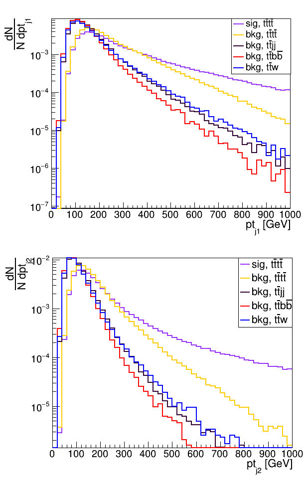
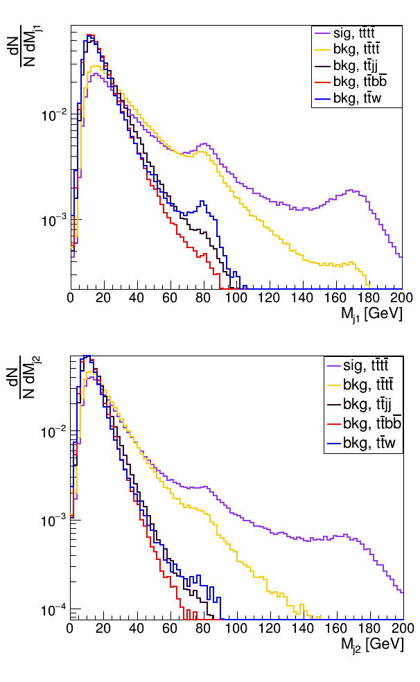
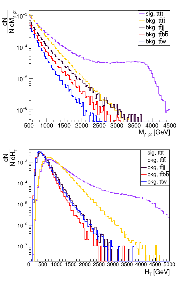
Figure 2: The signal (for $M_{G^{(1)}}$ = 4 TeV) and background distributions in $p_{T}$ of the leading and next-to-leading jets (left top and left bottom), the corresponding jet masses (middle top and middle bottom), the invariant mass of the two jets (right top) and $H_{T}$ (right bottom).

In Fig. 2, we display the distributions in the aforementioned variables for the leading backgrounds as well as the signal (for a typical value of the $G^{(1)}$-mass, namely 4 TeV). As expected, for the signal events, the $p_{T}$ of the two leading jets have a much broader distribution as compared to the backgrounds. As Fig. 2 suggests, a strong cut on the $p_{T}$s of the two leading jets would serve to suppress a much larger fraction of the two major backgrounds ($t\overline{t}jj$ and $t\overline{t}b\overline{b}$) as also the subleading ones than it would affect the signal. Understandably, the $p_{T}(j_{1})$ distribution of the SM 4-top background is the closest to the signal, a consequence of the somewhat similar event topologies. On the other hand, the corresponding $p_{T}(j_{2})$ distribution is much softer than that for the signal. This can be understood from the fact that while the “signal-like” events would largely correspond to the $G^{(1)}$ (on-shell or off-shell) decaying to two tops with relatively large and comparable $p_{T}$s (as indicated by the left-panels of Fig. 2). But for the SM-like 4-top sample, the absence of any heavy resonance makes the $p_{T}$ distribution of the next-to-leading jet much softer compared to the signal.

The very hardness of the two leading top-jets facilitates their reconstruction within a cone of radius $R=0.5$ (for a three-prong fatjet, the optimal choice being given by $\Delta R={3m_{j}}/{2p_{T}}$). For the signal events, the jet mass distribution for the two leading jets shows (see Fig. 2) three distinct peaks, where the one at low masses corresponds to $b$-jets or other secondary QCD radiation. The other two nontrivial peaks correspond to the $W$ boson mass and the $top$ itself when they are reconstructed within a radius of $R=0.5$. The SM 4-top background also shows a similar behavior for the leading jet, albeit with a less prominent peak around the top mass whereas the sub-leading jet for this background does not carry any evidence of a top-quark at all. This difference is but a consequence of the $p_{T}$ distribution for the second jet as discussed above. The other backgrounds have a prominent peak at low masses corresponding to the QCD radiation and drop rapidly as we move towards larger masses, with the only exception being $t\overline{t}W$ which shows a prominent peak at $W$ mass for the leading jet and a slightly obscured peak for the sub-leading jet.

Given the fact that the $p_{T}$ distributions are much harder (especially for the second jet) for the signal events, it is conceivable that this might be true as well for the other jets as well. Indeed, as Fig.2 shows, the variable $H_{T}$ (for the signal) has a much harder distribution as well. And although it is related, in a fashion, to the two aforementioned $p_{T}$ distributions, this variable obviously carries extra information and can, hence, be used as an independent discriminator.

Finally, for the signal, we also expect the invariant mass of the two most energetic top quarks to be centred around the $G^{(1)}$ mass, with the width of the distribution comparable to the decay width. This is illustrated by the plot for the invariant mass for the two leading jets, where the distribution shows a flat trajectory till large values of $M_{j_{1}j_{2}}$ (and falling off sharply once $M_{G^{(1)}}$ is crossed). This is expected to be accentuated further once the two leading jets can be associated with top quarks with greater certainty. On the other hand, the distributions for the other backgrounds drop rapidly as we go towards higher $M_{j_{1}j_{2}}$.

5.2.2 Subdominant discriminating Observables

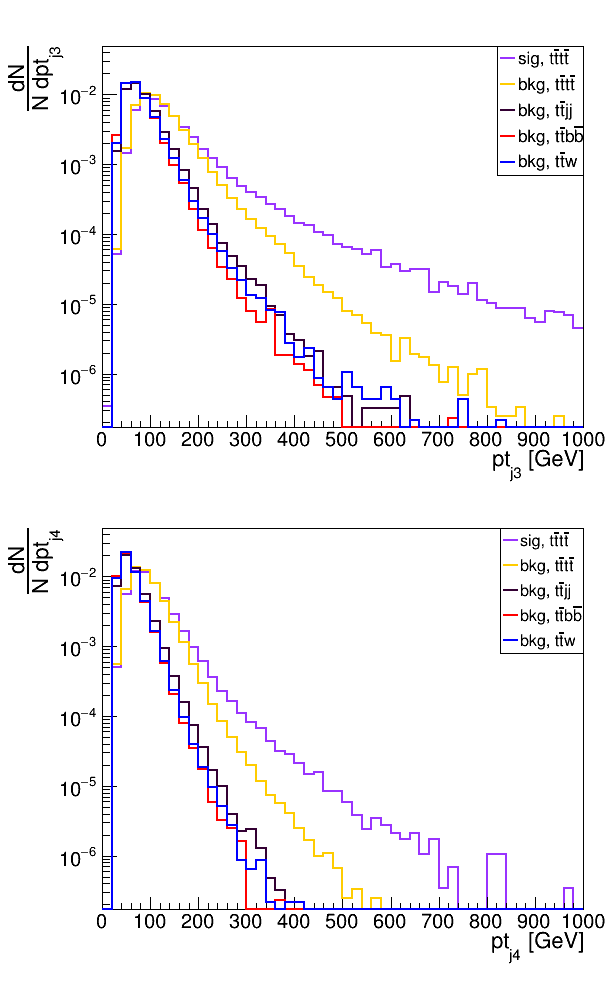
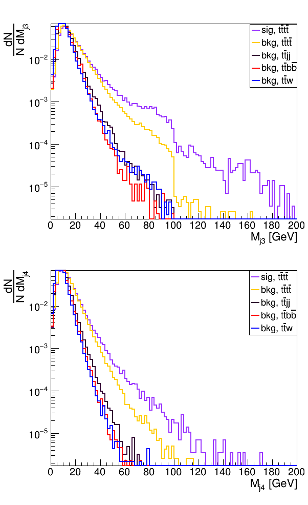
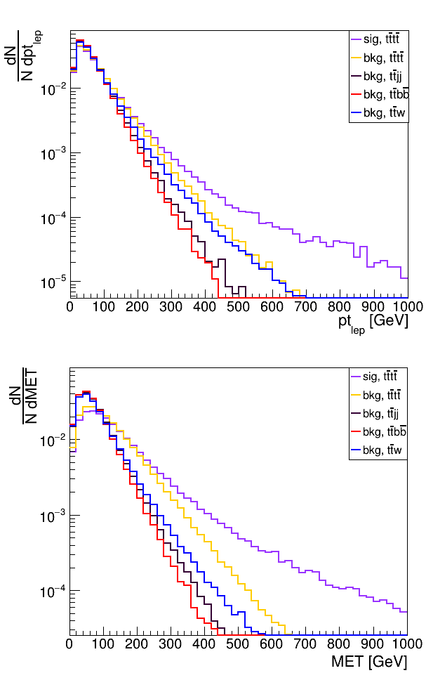
Figure 3: The signal (for $M_{G^{(1)}}$ = 4 TeV) and background distributions in $p_{T}$ of the third and fourth leading jets (left top and left bottom), the corresponding jet masses (middle top and middle bottom), the $p_{T}$ of the leading lepton (right top) and the missing transverse energy (right bottom).

In Fig 3, we display the distributions for a few observables which have relatively less discriminating power, namely the $p_{T}$ and jet mass of the third and fourth leading jet, $p_{T}$ of the leading lepton and transverse missing energy (MET). The last mentioned is expected to arise from the neutrinos accompanying the leptons, and, of course, is constructed from the imbalance in the measured $p_{T}$s of all the visible objects.

As seen from Fig. 3, the $W$ peak and/or the top peak in the jet mass are just about visible for the third jet, and cannot be discerned for the fourth. This is not unexpected, for the full event would have to be very energetic indeed for the third (or fourth) jet to carry sufficient energy to be sufficiently collimated and identified as a fatjet, given our choice of the jet radius. Indeed, the events where the third (or fourth) jet does have a high mass are largely those where the reconstruction process has clubbed together objects originating from disparate sources. Of course, there is also a small fraction wherein the tops emanating from the $G^{(1)}$ carry a lower $p_{T}$ (as compared to the other top/jets) and are not ranked as being the hardest (given our choice of using $p_{T}$ for ranking). In particular, for approximately 20$\%$ of all the events, a fatjet top is the third leading jet in $p_{T}$. And although the signal events boast wider distributions in both $p_{T}$ and jet-mass (understandably, the SM 4-top background is the closest to the signal on both these counts), it turns out that the discriminatory power is low (especially once the variables in the preceding subsection have been used.)

Much the same holds for the $p_{T}$ of the leading lepton as well as for the missing transverse momentum. In either case, the distribution for the signal is much wider (with the SM 4-top sample being somewhat similar) than the $t\overline{t}jj$ or $t\overline{t}b\overline{b}$ backgrounds. This can, again, be understood by realizing that, for the 4-top sample (whether signal or background), the leading lepton $p_{T}$ accrues in three steps, the $p_{T}$ of the decaying top (also see the preceding discussion about the third leading jet), hence the $p_{T}$ of the $W$ and, finally, the $p_{T}$ imparted by the decay of the $W$. For the $t\overline{t}W$ events, the first contribution does not exist. For the $t\overline{t}b\overline{b}$ and the $t\overline{t}jj$ samples, the leptons largely arise from the fragmentation (once the requirement of two fatjets is imposed) and are relatively softer. The same argument holds for the neutrino $p_{T}$ (the irreducible source of the MET). There is, of course, an additional contribution arising from jet $p_{T}$ measurements, but this, understandably, does not harden the spectrum substantially.

With the demand for two top-fatjets in the final state, it is tempting to consider observables characterising subjets within the fatjets. Observables such as N-subjettiness [47] and Energy Correlation functions [48] etc, however, do not improve the results because of the similar event topology for both the signal and the 4-top SM background (with the other backrounds being reduced substantially by the imposition of other cuts); rather, the imposition of cuts based on these only serve in worsening the discovery significance by reducing the number of signal events. Hence for the cut-based studies, we would not be using such observables.

Instead, we constrain the masses of the two fatjets to be around $m_{t}$. To be specific, we impose $100<m_{j_{1}/j_{2}}<250$ GeV, in order to maximise the retention of the signal. Furthermore, the lower cut not only removes the very large QCD radiation, but also the potentially significant $W$-fatjet background.

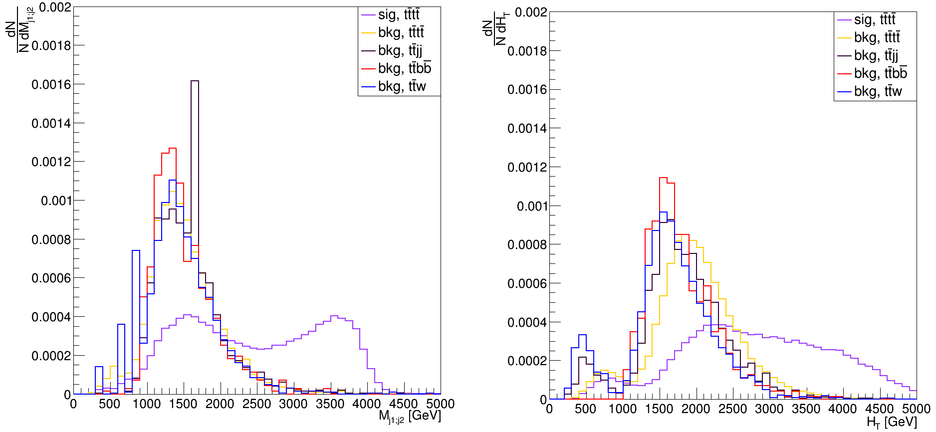
Figure 4: $M_{j_{1}j_{2}}$ and $H_{T}$ distribution after putting a cut of $100<m_{j1},m_{j2}<250$ GeV.

Once it has, thus, been ensured that the event contains two top-like fatjets, the distribution in the invariant masses of the two leading jets (see Fig. 4) is significantly different for the signal as compared to the backgrounds. For the former, the peak should ideally lie just at $M_{j_{1}j_{2}}=M_{G^{(1)}}$. However, there exists a slight degradation on account of the jet reconstruction algorithm losing a few entities (either on account of some neutrinos in hadronic decays or due to some hits not registering as part of the jet). The second peak at a lower $M_{j_{1}j_{2}}$ value might seem intriguing. This, however, is but an artefact of the cuts. Noting that, for a three-prong top-jet, the radius scales like $R=3~{}m_{j}/2p_{T}$, our twin choices of $R\leq 0.5$ and $m_{j}>100$ GeV essentially translates to $p_{T}>300$ GeV. With the invariant mass of the two leading jets being expressible as

$$M_{j_{1}j_{2}}^{2}=2\cosh(\Delta\eta)\sqrt{p_{T_{j_{1}}}^{2}+m_{j_{1}}^{2}}\sqrt{p_{T_{j_{2}}}^{2}+m_{j_{2}}^{2}}-2\cos(\Delta\phi)p_{T_{j_{1}}}p_{T_{j_{2}}}+m_{j_{1}}^{2}+m_{j_{2}}^{2}\ ,$$ (11)

this implies that the $M_{j_{1}j_{2}}$ distributions start only at around $500$ GeV. This explains the initial rise as seen in Fig. 4. However, with the $p_{T}$ distributions falling for higher $p_{T}$s (as seen in Fig. 2), a kinematic peak must result at relatively low $M_{j_{1}j_{2}}$. A cut of $M_{j_{1}j_{2}}>2000$ GeV would, thus, significantly enhance the signal to background ratio. Expectedly, the $H_{T}$ plot too shows clear distinction with the background showing a sharp peak around $1700$ GeV (for the same kinematic reason as $M_{j_{1}j_{2}}$), whereas the signal boasts a much flatter distribution extending till $5000$ GeV. In this case too, a cut of around $H_{T}>2000$ GeV would considerably improve the signal-to-noise ratio.

5.3 Analysis

Having gained an understanding of signal and background behaviour, we first proceed with a cut-based analysis. As discussed earlier, the dominant decay mode, viz. the fully hadronic decay of two of the tops (the other being required to result in fatjets) suffers from very large backgrounds (mainly from $t\overline{t}jj$ and, to a lesser extent, from $t\overline{t}b\overline{b}$). Concentrating on semileptonic decays addresses this problem by greatly reducing the $t\overline{t}jj$ background, with only a relatively small decrease (nominally, about by only a factor of about two-thirds, discounting efficiencies) in the signal strength. Hence, we concentrate on this mode. Below, we outline the detailed sequence of cuts we intend to apply.

• $\bf{Baseline~{}selection~{}cuts}$ : In order to reduce the $t\overline{t}jj$ and $t\overline{t}b\overline{b}$ background, we are looking for at least one isolated and hard (with a minimum $p_{T}$ of 20 GeV for the leading candidate) light lepton ($e^{\pm},\mu^{\pm}$). accompanied by a missing transverse momentum (MET) of at least 20 GeV. Furthermore, we demand that there be at least 6 jets in the event, with a minimum $p_{T}$ of 20 GeV each.

• $\bf{N_{fatjets}}$ : The two boosted tops because of their large transverse momenta can be confined within a jet radius of $R=0.5$, thereby constituting a fatjet. We demand that there be at least two fatjets with a jet mass satisfying $m_{j}\in[100,250]$ GeV.

• $\bf{N_{btags}}$: Once the two leading fatjets are isolated, we demand that a minimum of two of the other jets are b-tagged.

• $\bf{H_{T}}$: We demand that $H_{T}$ (the scalar sum of all hadronic $p_{T}$s) be greater than 2 TeV.

• $\bf{M_{fj_{1};fj_{2}}}$: Since the invariant mass of the two leading fatjets should roughly correspond to the RS gluon mass, we demand $M_{fj_{1};fj_{2}}>2$ TeV.

Cuts	Signal	${\bf t\overline{t}t\overline{t}}$ (SM)	${\bf t\overline{t}b\overline{b}}$	${\bf t\overline{t}jj}$	${\bf t\overline{t}W}$
${\bf Generation~{}level}$	2.21	15.7	$2.4\times 10^{4}$	$4.65\times 10^{5}$	602
${\bf Baseline~{}selection}$	0.672	4.96	$2.24\times 10^{3}$	$6.31\times 10^{4}$	61.3
${\bf N_{fatjets}\geq 2}$	0.032	0.029	0.156	12.6	0.025
${\bf N_{btags}\geq 2}$	0.014	0.014	0.0288	2.09	0.0033
${\bf H_{T}\geq 2~{}TeV}$	0.008	0.0018	0.0072	0.163	0.0004
${\bf M_{fj_{1};fj_{2}}\geq 2~{}TeV}$	0.006	0.0002	0.0029	0.023	0.0002

Table 1: Cut flow table for the cross section (in fb) for the one-lepton final state at $\sqrt{s}$ = 14 TeV. Signal corresponds to $M_{G^{(1)}}=4$ TeV and $\xi=5$.

As discussed earlier and as seen from Table 1, the largest reducible backgrounds are $t\overline{t}jj$, $t\overline{t}b\overline{b}$ and $t\overline{t}W$, in that order. The baseline selection cut reduces the signal by about 67%; on the other hand, the $t\overline{t}jj$ background is reduced by about $85~{}\%$ while the $t\overline{t}$$b\overline{b}$ and $t\overline{t}W$ backgrounds are reduced by nearly 90%. Demanding that the event contains at least two fatjets and atleast two b-tagged jets does reduce the signal by a factor of nearly 20, but the dominant backgrounds are suppressed by several orders of magnitude. At this stage, the (irreducible) SM $t\overline{t}t\overline{t}$ background is nearly the same as the signal size (for our benchmark point). Finally, once we demand a cut of 2 TeV on $H_{T}$ and the invariant mass of the two leading fatjets, the two largest backgrounds ($t\overline{t}jj$ and $t\overline{t}$$b\overline{b}$) comes down to manageable levels, whereas only a small amount of $t\overline{t}W$ survives. As far as the SM $t\overline{t}t\overline{t}$ is concerned, it is reduced by almost eight times compared to the surviving signal cross section. At a luminosity of $3000~{}fb^{-1}$, we get a total of 19 signal events compared to a total of 77 events for the background. This results in a significance ($\sigma={N_{s}}/\sqrt{N_{s+b}}$) of 1.84$\sigma$. As we move towards higher center-of-mass (c.o.m) energies in future LHC runs, we can probe more and more massive RS gluons.

6 Neural Network Analysis

6.1 Artificial Neural Network(ANN) Model

The artificial neural network (ANN) [49], is a recent machine learning technique inspired by the network and functioning of interconnected neurons in the human brain. It has been employed in tasks such as discriminating between signal and background events and identifying physics objects like b-tagging using collider experiment observables [50, 51, 52, 53, 54, 55, 56, 57, 58, 59, 60, 61, 62, 63, 64].

The process commences with the selection of features (typically, kinematic variables) from the collider experiment data, including both signal and background events, and training the ANN to detect patterns that would help it to differentiate between the two classes. ANNs consist of interconnected nodes, also called neurons, organized, typically, into three kinds of layers, viz. the Input layer, Hidden layers and the Output layer. A representative architecture of a feed-forward ANN with a single hidden layer is shown in Figure 5.

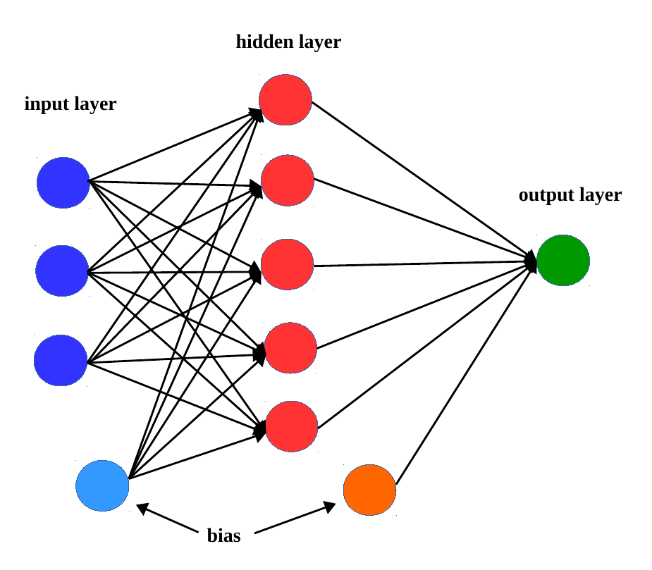
Figure 5: Representative architecture of a feed-forward artificial neural network for single hidden layer.

The selected features (collider observables in our case) are fed to the model through the input layer. These observables ($x_{i}$) are initially assigned random weights ($w_{ji}$) and then a bias ($b_{j}$) is added before passing the inputs through an activation function as in Eq. 12.

$$\sigma_{j} =\sum_{n}w_{ji}x_{i}+b_{j}$$ (12)

$$Y_{j} =\mathcal{F}(\sigma_{j}).$$

The activation functions ($Y_{j}$) introduce non-linearities into the network, and some common activation functions include the sigmoid, the hyperbolic tangent (tanh), and the rectified linear unit (ReLU). This processed output from the input layer is fed to the hidden layer, and the processed output from the latter, in turn, goes to the output layer. In case of a multiple hidden layered structure, the input of any hidden layer is the processed output from the previous hidden layer. This sequence of processing is known as Forward Propagation.

At this step, a cost function (loss function) is defined with the specific choice depending on the problem at hand. This calculates the difference between the predicted output and actual output, and minimizing this leads to the optimization of the network. Examples of the cost function include Mean Squared Error (MSE), Cross-Entropy Loss (Log Loss), Binary Cross-Entropy Loss (Logistic Loss), Total Variation Loss, etc

To minimize the loss function, the weights are updated through a process called backward propagation, typically achieved using the stochastic gradient descent algorithm. This consists of calculating the gradient of the loss function with respect to each weight, iteratively and layer by layer, and propagating backward from the last layer to avoid redundant computations of intermediate terms in the chain rule. The weights for the $(n+1)$-th epoch are updated using the weights $w^{n}_{ji}$ from the $n$-th epoch and the gradient of the cost function $f(\left\{w^{n}_{kl}\right\})$, namely

$$w^{n+1}_{ji}=w^{n}_{ji}-\alpha\,\frac{\partial}{\partial w^{n}_{ji}}\,f(\left\{w^{n}_{kl}\right\}),$$ (13)

where the learning rate $\alpha$ is a small positive constant that determines the step size of each update.

The observables are passed again through the model with these updated weights and the loss function values recalculated. One such complete single iteration through the entire training dataset during the training phase is called an epoch. This process continues until the model weights have been so updated as to minimize the loss function. Once the weight values reach such an optimal set, the trained model is ready to make predictions.

The architecture of neural networks, such as the number of hidden layers and neurons in each layer, along with the number of epochs, depends on factors like number of inputs, desired output, data complexity, error function intricacy, network design, and training algorithm. Insufficient epochs result in underfitting, missing data patterns, while excessive epochs lead to overfitting, causing specialization and poor generalization. Achieving the right balance is critical for optimal learning. Techniques like early stopping and regularization help find this balance.

6.2 ML architecture

In our scenario, the final state involves a minimum of 6 jets, which corresponds to at least 24 hadronic observables (comprising 3 momentum components and 1 invariant mass for each jet), along with 4 observables for the lepton as well as the missing transverse momentum (MET). Since such fundamental variables, in isolation, may or may not possess significant discriminatory power, it is a standard approach to work with a broader array of observables that exhibit greater discriminatory potential. Such strategic combinations of these fundamental observables could yield valuable insights, especially when applied within a neural network, whose primary role is to differentiate between the signal and background by assigning weights based on the discriminating capabilities of the observables (or combinations thereof). In this, we will use our understanding of kinematic distributions which we explored in the cut-based analysis (Section 5.1).

To produce the data (both signal and background) for our analysis, we begin by applying some initial criteria, which are outlined as follows:

$$n_{jets}\geq 4\hskip 14.22636pt{\rm and}\hskip 14.22636ptp_{T}^{jet}\,>\,20\,{\rm GeV}$$ (14)

$$n_{lep}>0\hskip 14.22636pt{\rm and}\hskip 14.22636ptp_{T}^{lep}\,>\,20\,{\rm GeV}$$

$${\rm MET}\,\ >\,20\,{\rm GeV}.$$

In this analysis, our focus is on 34 observables, which are further categorized into low-level observables, as shown in Table 2, and derived observables, as detailed in Table 3.

transverse momentum of the 4 leading jets	$p_{T}^{1}$, $p_{T}^{2}$, $p_{T}^{3}$, $p_{T}^{4}$
individual masses of the 4 leading jets	$m_{1}$, $m_{2}$, $m_{3}$, $m_{4}$
transverse momentum of the leading lepton	$p_{T}^{l}$
missing transverse energy	$E_{T}\!\!\!\!\!\!\,\,\!\!\!/$
rapidity of the 2 leading jets	$\eta_{1}$ and $\eta_{2}$
azimuthal angle of the 2 leading jets	$\phi_{1}$ and $\phi_{2}$
number of jets	$n_{jets}$
number of b-jets	$n_{b}$
Total	16 observables

Table 2: Low level observables for ANN training.

separation between two jets	$\Delta R_{j_{1}j_{2}}$, $\Delta R_{j_{1}j_{3}}$, $\Delta R_{j_{1}j_{4}}$, $\Delta R_{j_{2}j_{3}}$, $\Delta R_{j_{2}j_{4}}$, $\Delta R_{j_{3}j_{4}}$
invariant masses for the 3 leading jet pairs	$M_{j_{1}j_{2}},M_{j_{1}j_{3}}$, $M_{j_{2}j_{3}}$
scalar sum of transverse momentum of the jets	$H_{T}$
$\tau_{32}$ for the 4 leading jets	$\tau_{32}^{1}$, $\tau_{32}^{2}$, $\tau_{32}^{3}$, $\tau_{32}^{4}$
$\tau_{21}$ for the 4 leading jets	$\tau_{21}^{1}$, $\tau_{21}^{2}$, $\tau_{21}^{3}$, $\tau_{21}^{4}$
Total	18 observables

Table 3: Derived observables for ANN training.

Of the second set, the $\tau_{32}^{i}$ ($\tau_{21}^{i}$) observable for the $i$-th jet is given by $\tau_{3}/\tau_{2}$ ($\tau_{2}/\tau_{1}$), where the N-subjettiness $\tau_{N}$ is defined as

$$\tau_{N}=\frac{1}{d_{0}}\,\sum_{k}\,p_{T,k}\,{\rm min}\Big{(}\Delta R_{j_{1}j_{k}},\Delta R_{j_{1}j_{k}},....,\Delta R_{j_{N}j_{k}}\Big{)}.$$ (15)

Here $N$ is the number of candidate subjets of the jet to be reconstructed, $k$ runs over the constituent particles in a given jet with $p_{T,k}$ being their transverse momenta and $\Delta R_{j_{i}j_{k}}$, the angular separation between a candidate subjet $i$ and a constituent particle $k$. Furthermore,

$$d_{0}=\sum_{k}\,p_{T,k}\,R_{0},$$ (16)

where $R_{0}$($=0.5$) is the characteristic jet-radius. Physically, $\tau_{N}$ provides a dimensionless measure of whether a jet can be regarded to be composed of $N$-subjets. In particular, the ratios $\tau_{N}/\tau_{N-1}$ are powerful discriminants between jets predicted to have $N$ internal energy clusters and those with fewer clusters. For example, jets coming from the hadronic decays of the $Z/W/H$ tend to have lower values for the ratio $\tau_{21}\equiv\tau_{2}/\tau_{1}$ as compared to QCD or top-jets. Jets coming from the three-pronged hadronic decay of the tops have a low value of $\tau_{32}\equiv\tau_{3}/\tau_{2}$.

In order to reduce the $t\overline{t}jj$ cross-sections to manageable levels, which otherwise is disproportionately large, we demand that the (individual) masses of the two leading jets be greater than 80 GeV in addition to the baseline cuts used in Eq. 14. Its impact is shown in Table 16. After the cuts, it has to be ensured that there are enough events for signal as well as background to be fed to the ANN. We have taken sufficiently large and equal sample sizes for both, so that the network is able to predict the characteristics more accurately.

Cuts	Signal	${\bf t\overline{t}t\overline{t}}$	${\bf t\overline{t}b\overline{b}}$	${\bf t\overline{t}jj}$	${\bf t\overline{t}w}$
Generation level	2.21	15.7	$2.4\times 10^{4}$	$4.65\times 10^{5}$	602
Baseline selection (Eq. 14)	0.839	5.19	$1.82\times 10^{3}$	$6.29\times 10^{4}$	56.4
${\bf m_{1,2}>}$ 80 GeV	0.0942	0.0917	0.45	41.463	0.117

Table 4: Cut flow table of signal and background cross sections (in fb) pertaining to the preselections for the ANN at $\sqrt{s}$ = 14 TeV. Signal corresponds to $M_{G^{(1)}}=4$ TeV and $\xi=5$.

Unlike traditional cut-based collider analyses that rely heavily on multitude of cuts to reduce background events, we employ only a set of basic cuts, mentioned in Eq. 14 and Table 16, to eliminate obviously background-like events while ensuring fairness and compatibility with the ANN methodology. These cuts are essential as they filter out events that contribute significantly to the total cross-section for the respective channels but provide little discriminating ability. In this instance, demanding a higher invariant mass for the two leading jets helps eliminate the softer QCD emissions, allowing the neural network to focus solely on the relevant events for signal and background discrimination. This approach prevents the network from learning unnecessary features and allows it to assign appropriate weights to relevant events, thereby ensuring faster and better convergence.

These input observables have varying ranges. To ensure that the gradient descent method progresses smoothly towards the minima, and that the steps for it are updated uniformly across all features, we normalize the data before inputting it to the model. This, typically, involves scaling the data between 0 and 1, and is often referred to as Min-Max scaling. Such a normalization allows for a uniform application of the gradients in the hidden layer as well as recombination of observables into newer sets, thereby facilitating a smoother functioning of the network.

Our objective here is to distinguish between signal and background, making it a binary classification task. Signal events are thus categorized as 1, while the Standard Model (SM) background events are denoted as 0. The optimization goal is to achieve high accuracy in discriminating between signal and background in the testing sample, followed by achieving an appropriate level of significance.

Following the training of the neural network, it is possible to assess the significance of each feature in the analysis. Feature importances can be evaluated on both global and local scales. Global feature importance assesses the utility of a feature across the entire dataset, while local feature importance pertains to a single prediction, such as an individual data point or event. To interpret the model, we have chosen to utilize SHAP (SHapley Additive exPlanations) [65], a local feature attribution technique based on Shapley values. It quantifies the importance of a feature by determining how effectively the model predicts a specific class when the feature is present compared to when it is absent within the comprehensive set of features. For a given feature, SHAP takes into account not only that feature but also the potential interactions among the features, considering that correlations may exist among them. It calculates the Shapley values $\phi_{i}$ using [65, 66]

$$\phi_{i}=\sum_{S\subseteq N\backslash\{i\}}\ \frac{|S|!(M-|S|-1)!}{M!}\ [f_{x}(S\cup\{i\})-f_{x}(S)]\ .$$ (17)

Here, $i$ represents the feature for which the SHAP value is being determined, $N$ is the collection of all features, and $M$ denotes the total number of features. The variable $S$ represents a subset of $N$ that excludes feature $i$. The function $f_{x}$ corresponds to the model’s prediction. Consequently, the algorithm calculates a weighted sum of the differences in model predictions, considering the presence or absence of the $i^{th}$ feature for all feasible combinations of the subset $S$.

6.3 NN Training

The construction of the ANN model utilizes the Keras library in conjunction with TensorFlow for backend implementation. This is designed to classify the contribution of signals versus Standard Model (SM) background events. For the purpose of testing and validation, an equal number of samples are randomly selected from the pools of signal and background data. The training set is subjected to random shuffling, and the input data is subsequently supplied to the network.

For our dataset, we generated 100,000 each of signal and SM background events, the latter receiving contributions from processes like $t\overline{t}t\overline{t}$, $t\overline{t}jj$, $t\overline{t}b\overline{b}$, and $t\overline{t}W$, with proportions determined by their respective cross-sections. The events are mixed randomly, and 20% of them are designated for testing, while the remaining 80% is divided into two subsets. Within these subsets, 80% is allocated for training, and the remaining 20% is used for validation.

The activation function used in case of hidden layers is ReLU (Rectifier Linear Unit)[67] and softmax for the output layer. The Adam (Adaptive Moment Estimation) optimizer[68] is used to minimize the loss-function between the input and output. The Adam optimization algorithm is an extension of the stochastic gradient descent that computes individual adaptive learning rates for different parameters from estimates of first and second moments of the gradients to update network weights iterative based in training data. Finally, for the loss function, we have used the binary cross-entropy function, which is defined as

$$H(y,p) = -\frac{1}{N}\,\sum_{i=1}^{N}\,(y_{i}\cdot\log(p(y_{i}))+(1-y_{i})\cdot\log(1-p(y_{i}))).$$ (18)

Here $y_{i}$ denotes the true label for the observables (either 0 or 1 for the background and signal respectively), $p(y_{i})$ is the predicted probability that the instance belongs to class 1 (signal) and $N$ represents the span of the data-set.

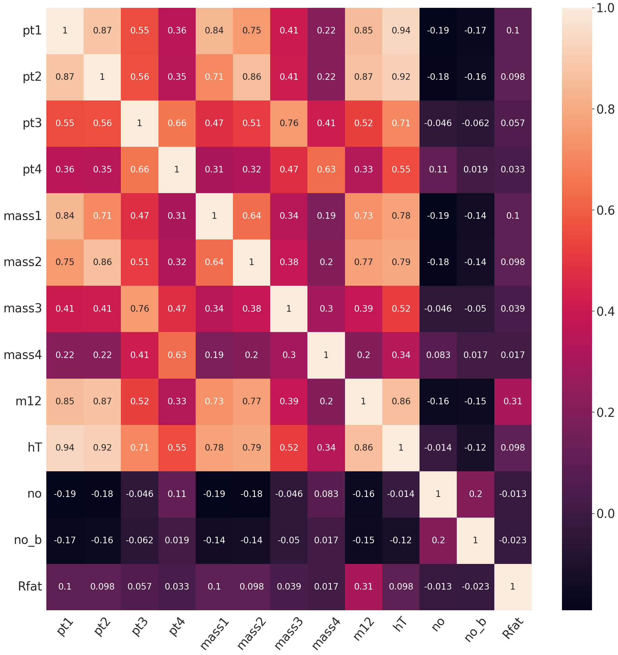
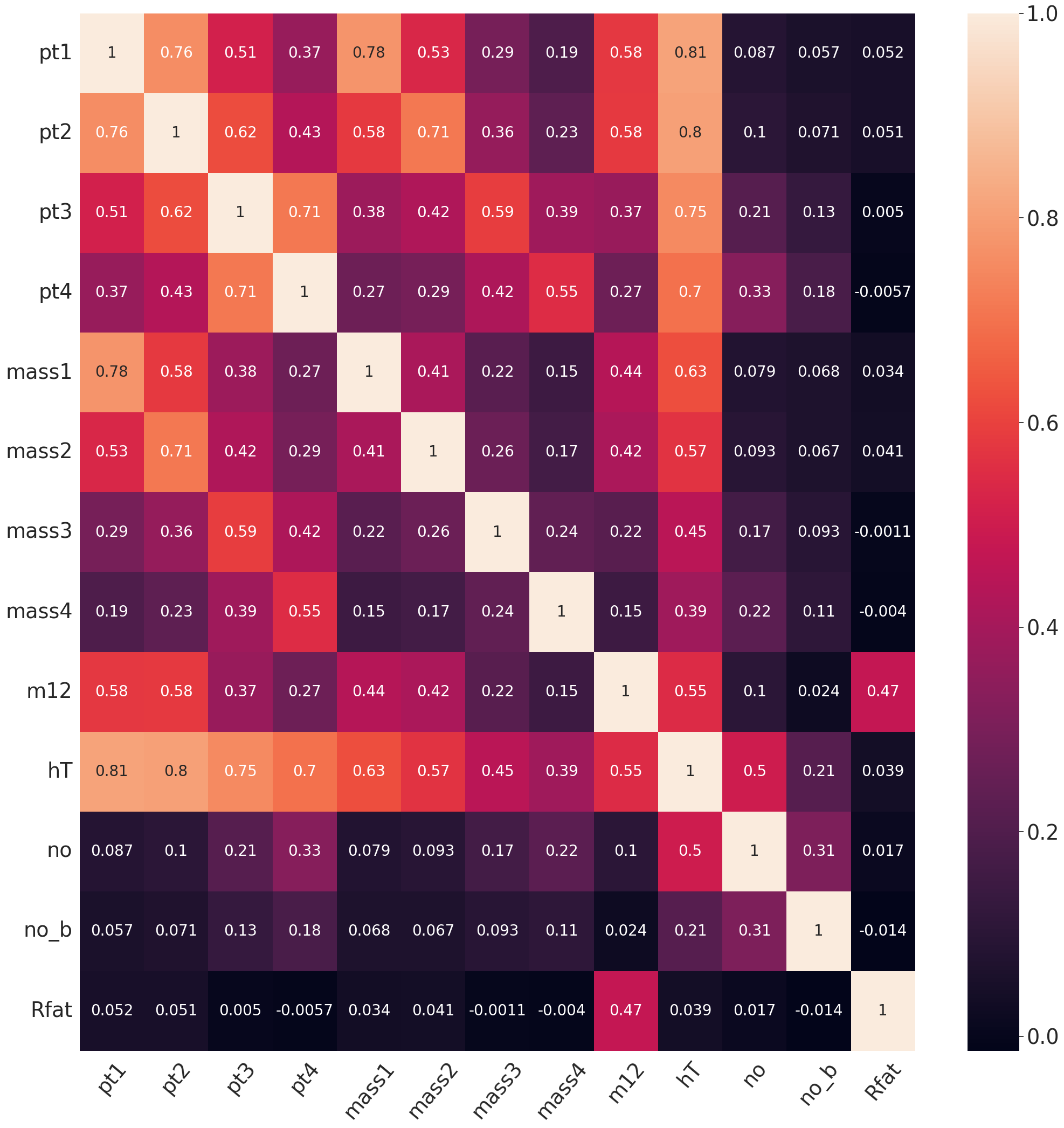
Figure 6: The correlation plots between the observables for $\sqrt{s}$ = 14 TeV for signal (left) and background (right) respectively with $M_{G^{(1)}}$ = 4 TeV.

In Figure 6, we have illustrated the relationships among some of the observables that serve as inputs to the machine learning network. The plot reveals that certain observables exhibit modest correlations with each other, making them suitable features for the discrimination training process.

However, there are other observables where the correlation is notably pronounced. In these cases, the extent of correlation may vary between signal and background. For instance, consider the correlation between $H_{T}$ and $M_{12}$ (referred to as hT and m12 respectively in Figure 6). In this particular scenario, the correlation between these two observables is substantial for signal, while it is comparatively weaker for the background. This difference can serve as an effective discriminator.

Our analysis also incorporates batch normalization [69], a technique that normalizes the layers within the network to enhance training while maintaining consistent accuracy levels. Notably, we have obtained similar results for both the analyses, whether with or without batch normalization and therefore have presented the figures and findings that include batch normalization. We also experimented with standardization, a scaling method applied to various data features. However, this did not yield any noticeable changes in the results. In addition, we use the dropout regularisation technique [70] to prevent an overfitting of the model. It works by randomly dropping out a certain fraction (which depends on the dropout rate) of neurons in a layer during each forward and backward pass. The details of the full ANN structure incorporated in the analysis is given in Table 5.

Input	Observables
Layers	dense layer : 50
	dropout layer (0.3)
	batch normalization layer
	dense layer : 20
	dropout layer (0.3)
	batch normalization layer
	dense layer : 5
	dropout layer (0.2)
Layers setting	hidden layer activation = relu
	output layer activation = softmax
Compilation	loss = binary_crossentropy
	optimizer = adam[68]
	metric = accuracy

Table 5: ANN structure specifications.

Furthermore, we utilized a hyperparameter tuning technique called GridSearchCV. This approach involves testing various combinations of parameters provided through a list of dictionaries, including batch size and the number of training epochs. The objective here is to determine the optimal parameters for building the neural network, which can significantly impact its performance.

6.4 ANN results

A network’s capability of accurately differentiating between signal and background events is quantified through a metric known as the accuracy score. In the present instance, the network has been trained for the discrimination of signal events from background events, considering all background sources in accordance with their respective cross-section ratios for a luminosity of 3000 fb^-1. The outcome of this training demonstrates an accuracy level as high as $\sim$89.5%. We have plotted the accuracy versus the number of epochs plot upto 1000 epochs in Fig 7. Also shown is the variation in the loss over the same number of epochs. As can be observed, the accuracy saturates for smaller values of epochs and the difference between the training and validation accuracy keeps on increasing with epochs. For more epochs, the validation accuracy starts to reduce, as a result of overtraining. A similar pattern follows for the loss as well.

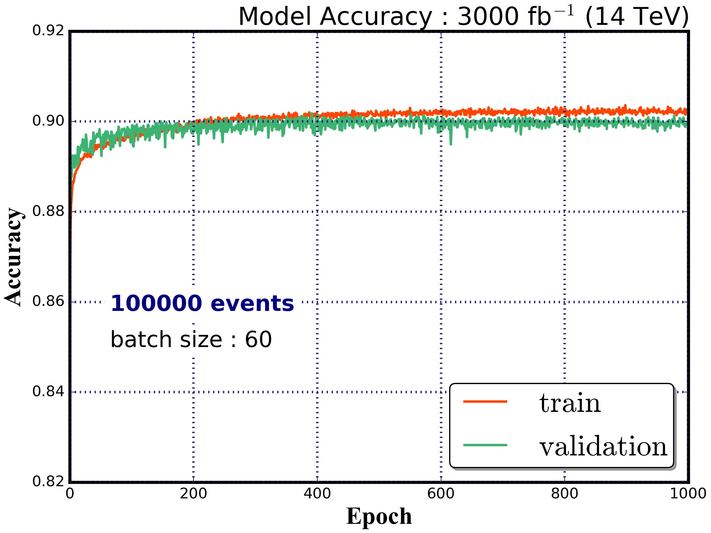
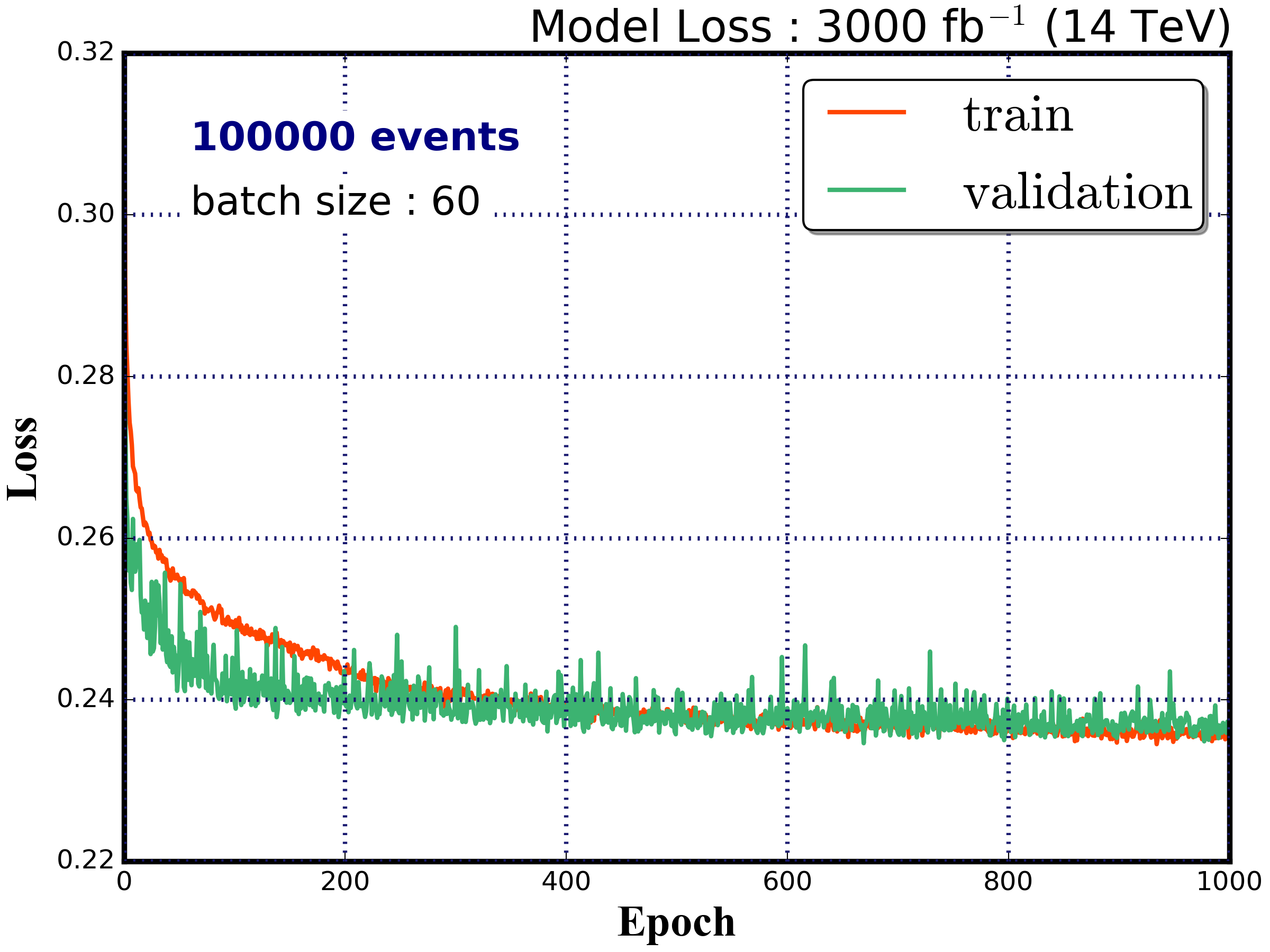
Figure 7: The variation of model training and validation accuracy (loss) with epochs on the left (right) hand side plot for $\sqrt{s}$ = 14 TeV corresponding to $M_{G^{(1)}}$ = 4 TeV with batch size 60.

Figure 8 illustrates the SHAP values, as introduced in Section 6.2 and described by Eq. 17. On the left plot’s $y$-axis, the feature names (observables) are arranged in order of importance from top to bottom. Meanwhile, the $x$-axis represents the SHAP value, with positive values indicating contributions that increase the prediction and negative values indicating contributions that decrease it. In the graph, each data point corresponds to an original dataset entry, and its color signifies the value of the associated feature. Red points represent high feature values, while blue points represent low values. For instance, for the most important feature $H_{T}$, we notice that the red points correspond to positive SHAP values, suggesting that a higher $H_{T}$ value positively impacts the network’s predictions compared to when $H_{T}$ is lower. This aligns with what we observed in the cut-based analysis in Section 5.3 where increasing the $H_{T}$ threshold significantly reduced the background. On the other hand, considering “tau321” (representing $\tau_{32}$ of the leading jet), a low value of this observable improves the network’s performance. This is logical in the boosted regime because the leading top can form a fatjet with three prongs, resulting in a smaller $\tau_{32}$ value. Since we do not anticipate the background to be highly boosted, a three-prong fatjet is less likely to occur, causing the $\tau_{32}$ of the leading jet to be larger than the signal. Analogous interpretations can be drawn for the other observables in a similar manner.

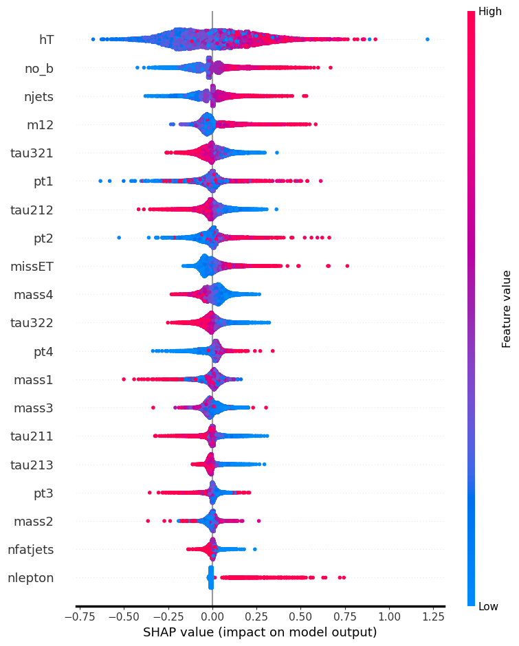
Figure 8: A summary plot showing the variation of SHAP values with the input feature values for the top 20 variables from the signal versus all the relevant backgrounds.

In addition to accuracy and feature importance, another essential evaluation tool is the Receiver Operating Characteristic (ROC) curve. ROC curves offer a visual representation of an algorithm’s performance, illustrating how well it separates the two classes. The area under the ROC curve (AUC) is a valuable performance metric, providing a single numerical value that quantifies the model’s ability to distinguish between classes. In the context of this analysis, the AUC-ROC curves are depicted in Figure 9. These curves offer insights into the network’s discriminative power and provide a basis for evaluating its performance in practical conditions.

In practical terms, the network’s performance can be further assessed by calculating the signal significance. This measure accounts for the sensitivity of the model in real-world scenarios, where the trade-off between signal and background discrimination is crucial for making meaningful discoveries in particle physics or similar fields. We achieve this through the optimisation of the selection criteria for the output discriminant by carefully choosing a cut-off point, denoted as $Y_{\rm cut}$, that maximizes the significance of our analysis. The variation of the final significance with respect to $Y_{\rm cut}$ is shown in the second plot of Figure 9. Notably, the exceptionally high cross-section of the $t\overline{t}jj$ background process compels us to contemplate an extreme value for $Y_{\rm cut}$.

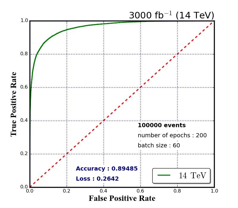
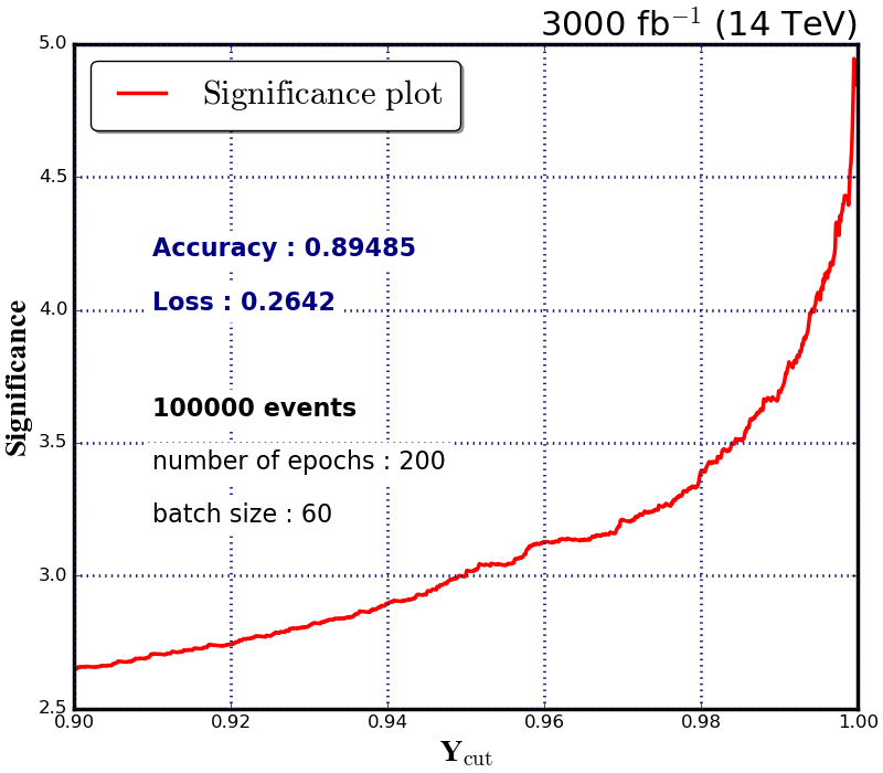
Figure 9: AUC-ROC curve (left) and significance (right) respectively for $\sqrt{s}$ = 14 TeV analysis with $M_{G^{(1)}}$ = 4 TeV corresponding to accuracy of 89.5%.

A comparison between the current network-based approach and the traditional cut-based technique performed earlier makes a strong case for the former. In the context of the cut-based method, the final count yields approximately 19 signal events and 77 background events, which corresponds to significance less than 2$\sigma$. However, when the artificial neural network (ANN) is employed, we get 150 signal events and 1228 background events with significance of 4.05 at $Y_{\rm cut}$ = 99.5%. With even larger values of $Y_{\rm cut}$, the ANN method yields a significantly higher significance of more than 4 as shown in Figure 9. This signifies the network’s exceptional ability to enhance the signal-to-noise discrimination and deliver improved results when compared to the cut-based approach, where the signal significance is less pronounced.

7 Summary and Conclusion

There are a plethora of models where heavy colored gauge bosons exhibit enhanced interactions with certain Standard Model (SM) fermions, most notably the top quark. This phenomenon is commonly associated with the pursuit of a dynamical explanation for Electroweak Symmetry Breaking (EWSB), especially in generic models like those incorporating extended color symmetry with colorons or axigluons as the mediators. For models constructed in higher dimensions, such states arise naturally as Kaluza-Klein modes of the gluon. In particular, within the bulk Randall-Sundrum scenarios, such KK-gluons have non-trivial wavefunctions along the fifth (bulk) direction, typically resulting in suppressed couplings with the light quark flavours. On the other hand, the right-handed top-quark being localized close to the infrared brane, has an enhanced coupling with the KK-gluons.

The large masses of such bosons renders pair-production cross sections to be small. Similarly, single production cross section is small too, owing to the suppressed coupling with a light quark-pair or a gluon-pair. Both these facts, as well as the typically large SM backgrounds, thus, call for other modes. Concentrating on the first of the KK-gluons (as they are well-separated), namely, the $G^{(1)}$, a particularly interesting mode at the LHC is associated production with a top pair, viz., $gg\to t\overline{t}G^{(1)}$, with the KK-gluon subsequently going into a top-pair, thereby leading preferentially to a four-top final state.

While the large $t\overline{t}G^{(1)}$ coupling facilitates this mode, it also leads to the KK-gluon having a naturally large width, and the commonly used narrow width approximation is often insufficient to capture its behavior accurately. Given this, we need to include at least the one-loop renormalised $G^{(1)}$ propagator.

The large mass of the $G^{(1)}$ typically results in both of the $t\overline{t}$ pair coming off it to be highly boosted. Consequently, their decay products tend to be collimated, resulting in a pair of top-fatjets. Of the other two tops, we require one of them to decay hadronically and the other leptonically. Thus, our final state of choice comprises of at least six jets (of which two are top-like fatjets, and another two are $b$-tagged), one hard and isolated lepton ($e^{\pm}/\mu^{\pm}$) and substantial missing transverse momentum.

We begin our analysis with a conventional cut-based approach. A careful study of the signal and background profiles shows us that only a handful of kinematical variables are powerful discriminating tools. These are the transverse momenta of the two leading jets, their individual jet masses, the scalar sum of all the jet transverse momenta, and, to a reduced extent, the transverse momentum of the lepton. Of course, the invariant mass of the two leading jets is expected to be another powerful tool as, for the signal-events, it is expected to peak near the $M_{G^{(1)}}$. However, this is tempered to a great degree by the aforementioned very large width of the $G^{(1)}$, and prevents reaching large significance values. The higher cross sections of the background, specially the $t\overline{t}jj$, worsens things further.

This challenge has enticed us to explore the application of machine learning methods. We study here the most basic of them all, Artificial Neural Networks (ANNs), to enhance the discrimination power. To expedite the convergence of the neural network in this discrimination task, we have implemented some basic cuts. The background sample is created by adding the relevant background processes in proportions determined by their cross-sections. In order for the network to effectively learn all the topological features of the signal and background, we provide 16 low level observables and 18 derived observables as inputs. Even though most of the observables play a role in this discrimination, we find that $H_{T}$, number of $b$-jets, total number of jets, invariant mass of the two leading jet-pairs ($m_{j_{1}j_{2}}$) and $\tau_{32}$ of the leading jet are the five most influential features in the process. The accuracy achieved by the network turns out to be $\sim 90\%$, which is a testament of its excellent learning capability. Moreover, the output discriminant exhibits significances in excess of 4$\sigma$, making it superior to conventional cut-based analysis. Use of more sophisticated modern machine-learning techniques would understandably push these limits higher, rendering the exploration of the four-top channel examined here worthy of further investigation at the LHC.

References

- [1] Christopher T. Hill and Elizabeth H. Simmons. Strong Dynamics and Electroweak Symmetry Breaking. Phys. Rept., 381:235–402, 2003. [Erratum: Phys.Rept. 390, 553–554 (2004)].
- [2] Christopher T. Hill and Stephen J. Parke. Top production: Sensitivity to new physics. Phys. Rev. D, 49:4454–4462, 1994.
- [3] Christopher T. Hill. Topcolor: Top quark condensation in a gauge extension of the standard model. Phys. Lett. B, 266:419–424, 1991.
- [4] Christopher T. Hill. Topcolor assisted technicolor. Phys. Lett. B, 345:483–489, 1995.
- [5] R. S. Chivukula, Andrew G. Cohen, and Elizabeth H. Simmons. New strong interactions at the Tevatron? Phys. Lett. B, 380:92–98, 1996.
- [6] Elizabeth H. Simmons. Coloron phenomenology. Phys. Rev. D, 55:1678–1683, 1997.
- [7] Paul H. Frampton and Sheldon L. Glashow. Chiral Color: An Alternative to the Standard Model. Phys. Lett. B, 190:157–161, 1987.
- [8] Paul H. Frampton and Sheldon L. Glashow. Unifiable Chiral Color With Natural Gim Mechanism. Phys. Rev. Lett., 58:2168, 1987.
- [9] Lisa Randall and Raman Sundrum. A Large mass hierarchy from a small extra dimension. Phys. Rev. Lett., 83:3370–3373, 1999.
- [10] H. Davoudiasl, J. L. Hewett, and T. G. Rizzo. Bulk gauge fields in the Randall-Sundrum model. Phys. Lett. B, 473:43–49, 2000.
- [11] Yuval Grossman and Matthias Neubert. Neutrino masses and mixings in nonfactorizable geometry. Phys. Lett. B, 474:361–371, 2000.
- [12] Tony Gherghetta and Alex Pomarol. Bulk fields and supersymmetry in a slice of AdS. Nucl. Phys. B, 586:141–162, 2000.
- [13] Stephan J. Huber and Qaisar Shafi. Fermion masses, mixings and proton decay in a Randall-Sundrum model. Phys. Lett. B, 498:256–262, 2001.
- [14] Alex Pomarol. Gauge bosons in a five-dimensional theory with localized gravity. Phys. Lett. B, 486:153–157, 2000.
- [15] Sanghyeon Chang, Junji Hisano, Hiroaki Nakano, Nobuchika Okada, and Masahiro Yamaguchi. Bulk standard model in the Randall-Sundrum background. Phys. Rev. D, 62:084025, 2000.
- [16] Tony Gherghetta. A Holographic View of Beyond the Standard Model Physics. In Theoretical Advanced Study Institute in Elementary Particle Physics: Physics of the Large and the Small, pages 165–232, 2011.
- [17] Mathew Thomas Arun and Debajyoti Choudhury. Bulk gauge and matter fields in nested warping: I. the formalism. JHEP, 09:202, 2015.
- [18] Mathew Thomas Arun and Debajyoti Choudhury. Bulk gauge and matter fields in nested warping: II. Symmetry Breaking and phenomenological consequences. JHEP, 04:133, 2016.
- [19] Mathew Thomas Arun, Debajyoti Choudhury, and Divya Sachdeva. Universal Extra Dimensions and the Graviton Portal to Dark Matter. JCAP, 10:041, 2017.
- [20] Arun Mathew Thomas and Debajyoti Choudhury. Neutron oscillation and baryogenesis from six dimensions. Phys. Rev. D, 106(3):L031701, 2022.
- [21] A. Akshay and Mathew Thomas Arun. Flavor-violating charged lepton decays in the little Randall-Sundrum model. Phys. Rev. D, 107(1):015013, 2023.
- [22] M. Guchait, F. Mahmoudi, and K. Sridhar. Tevatron constraint on the Kaluza-Klein gluon of the Bulk Randall-Sundrum model. JHEP, 05:103, 2007.
- [23] Kaustubh Agashe, Alexander Belyaev, Tadas Krupovnickas, Gilad Perez, and Joseph Virzi. Cern lhc signals from warped extra dimensions. Phys. Rev. D, 77:015003, Jan 2008.
- [24] Ben Lillie, Lisa Randall, and Lian-Tao Wang. The Bulk RS KK-gluon at the LHC. JHEP, 09:074, 2007.
- [25] Debajyoti Choudhury, Rohini M. Godbole, Ritesh K. Singh, and Kshitij Wagh. Top production at the Tevatron/LHC and nonstandard, strongly interacting spin one particles. Phys. Lett. B, 657:69–76, 2007.
- [26] Debajyoti Choudhury, Rohini M. Godbole, and Pratishruti Saha. Dijet resonances, widths and all that. JHEP, 01:155, 2012.
- [27] Rafel Escribano, Mikel Mendizabal, Mariano Quirós, and Emilio Royo. On Broad Kaluza-Klein Gluons. JHEP, 05:121, 2021.
- [28] Luc Darmé, Benjamin Fuks, and Fabio Maltoni. Top-philic heavy resonances in four-top final states and their EFT interpretation. JHEP, 21:143, 2020.
- [29] Qing-Hong Cao, Jun-Ning Fu, Yandong Liu, Xiao-Hu Wang, and Rui Zhang. Probing top-philic new physics via four-top-quark production. Chin. Phys. C, 45(9):093107, 2021.
- [30] Kaustubh Agashe, Gilad Perez, and Amarjit Soni. Flavor structure of warped extra dimension models. Phys. Rev. D, 71:016002, 2005.
- [31] Kaustubh Agashe, Antonio Delgado, Michael J. May, and Raman Sundrum. RS1, custodial isospin and precision tests. JHEP, 08:050, 2003.
- [32] Adam Falkowski, Martín González-Alonso, and Kin Mimouni. Compilation of low-energy constraints on 4-fermion operators in the SMEFT. JHEP, 08:123, 2017.
- [33] Kaustubh Agashe, Roberto Contino, Leandro Da Rold, and Alex Pomarol. A Custodial symmetry for . Phys. Lett. B, 641:62–66, 2006.
- [34] Marcela Carena, Eduardo Ponton, Jose Santiago, and Carlos E. M. Wagner. Light Kaluza Klein States in Randall-Sundrum Models with Custodial SU(2). Nucl. Phys. B, 759:202–227, 2006.
- [35] Debajyoti Choudhury, Timothy M. P. Tait, and C. E. M. Wagner. Probing heavy Higgs boson models with a TeV linear collider. Phys. Rev. D, 65:115007, 2002.
- [36] Rikkert Frederix, Davide Pagani, and Marco Zaro. Large NLO corrections in and hadroproduction from supposedly subleading EW contributions. JHEP, 02:031, 2018.
- [37] Ezequiel Alvarez, Darius A. Faroughy, Jernej F. Kamenik, Roberto Morales, and Alejandro Szynkman. Four tops for LHC. Nucl. Phys. B, 915:19–43, 2017.
- [38] G. Bevilacqua, M. Czakon, C. G. Papadopoulos, and M. Worek. Dominant qcd backgrounds in higgs boson analyses at the lhc: A study of jets at next-to-leading order. Phys. Rev. Lett., 104:162002, Apr 2010.
- [39] G. Bevilacqua, M. Czakon, C. G. Papadopoulos, R. Pittau, and M. Worek. Assault on the NLO Wishlist: pp — t anti-t b anti-b. JHEP, 09:109, 2009.
- [40] A. Bredenstein, A. Denner, S. Dittmaier, and S. Pozzorini. NLO QCD corrections to pp — t anti-t b anti-b + X at the LHC. Phys. Rev. Lett., 103:012002, 2009.
- [41] Adam Alloul, Neil D. Christensen, Céline Degrande, Claude Duhr, and Benjamin Fuks. FeynRules 2.0 - A complete toolbox for tree-level phenomenology. Comput. Phys. Commun., 185:2250–2300, 2014.
- [42] Neil D. Christensen and Claude Duhr. FeynRules - Feynman rules made easy. Comput. Phys. Commun., 180:1614–1641, 2009.
- [43] Johan Alwall, Michel Herquet, Fabio Maltoni, Olivier Mattelaer, and Tim Stelzer. MadGraph 5 : Going Beyond. JHEP, 06:128, 2011.
- [44] Richard D. Ball et al. Parton distributions for the LHC Run II. JHEP, 04:040, 2015.
- [45] Torbjorn Sjostrand, Stephen Mrenna, and Peter Z. Skands. PYTHIA 6.4 Physics and Manual. JHEP, 05:026, 2006.
- [46] J. de Favereau, C. Delaere, P. Demin, A. Giammanco, V. Lemaître, A. Mertens, and M. Selvaggi. DELPHES 3, A modular framework for fast simulation of a generic collider experiment. JHEP, 02:057, 2014.
- [47] Jesse Thaler and Ken Van Tilburg. Identifying Boosted Objects with N-subjettiness. JHEP, 03:015, 2011.
- [48] Andrew J. Larkoski, Gavin P. Salam, and Jesse Thaler. Energy Correlation Functions for Jet Substructure. JHEP, 06:108, 2013.
- [49] Yann LeCun, Yoshua Bengio, and Geoffrey Hinton. Deep learning. Nature, 521:436–444, 2015.
- [50] Jacob Searcy, Lillian Huang, Marc-André Pleier, and Junjie Zhu. Determination of the polarization fractions in using a deep machine learning technique. Phys. Rev. D, 93(9):094033, 2016.
- [51] Junho Lee, Nicolas Chanon, Andrew Levin, Jing Li, Meng Lu, Qiang Li, and Yajun Mao. Polarization fraction measurement in same-sign WW scattering using deep learning. Phys. Rev. D, 99(3):033004, 2019.
- [52] Junho Lee, Nicolas Chanon, Andrew Levin, Jing Li, Meng Lu, Qiang Li, and Yajun Mao. Polarization fraction measurement in ZZ scattering using deep learning. Phys. Rev. D, 100(11):116010, 2019.
- [53] K. Lasocha, E. Richter-Was, D. Tracz, Z. Was, and P. Winkowska. Machine learning classification: Case of Higgs boson CP state in decay at the LHC. Phys. Rev. D, 100(11):113001, 2019.
- [54] Leif Lonnblad, Carsten Peterson, and Thorsteinn Rognvaldsson. Using neural networks to identify jets. Nucl. Phys. B, 349:675–702, 1991.
- [55] V. Innocente, Y. F. Wang, and Z. P. Zhang. Identification of tau decays using a neural network. Nucl. Instrum. Meth. A, 323:647–656, 1992.
- [56] Bob Holdom and Qi-Shu Yan. Searches for the of a fourth family. Phys. Rev. D, 83:114031, 2011.
- [57] Alexander Radovic, Mike Williams, David Rousseau, Michael Kagan, Daniele Bonacorsi, Alexander Himmel, Adam Aurisano, Kazuhiro Terao, and Taritree Wongjirad. Machine learning at the energy and intensity frontiers of particle physics. Nature, 560(7716):41–48, 2018.
- [58] Pierre Baldi, Peter Sadowski, and Daniel Whiteson. Searching for Exotic Particles in High-Energy Physics with Deep Learning. Nature Commun., 5:4308, 2014.
- [59] Jie Ren, Lei Wu, Jin Min Yang, and Jun Zhao. Exploring supersymmetry with machine learning. Nucl. Phys. B, 943:114613, 2019.
- [60] Murat Abdughani, Jie Ren, Lei Wu, and Jin Min Yang. Probing stop pair production at the LHC with graph neural networks. JHEP, 08:055, 2019.
- [61] Raban Iten, Tony Metger, Henrik Wilming, Lídia del Rio, and Renato Renner. Discovering physical concepts with neural networks. Phys. Rev. Lett., 124:010508, Jan 2020.
- [62] Jie Ren, Lei Wu, and Jin Min Yang. Unveiling CP property of top-Higgs coupling with graph neural networks at the LHC. Phys. Lett. B, 802:135198, 2020.
- [63] Yu-Chen Guo, Li Jiang, and Ji-Chong Yang. Detecting anomalous quartic gauge couplings using the isolation forest machine learning algorithm. Phys. Rev. D, 104(3):035021, 2021.
- [64] Ji-Chong Yang, Yu-Chen Guo, and Li-Hua Cai. Using a nested anomaly detection machine learning algorithm to study the neutral triple gauge couplings at an collider. Nucl. Phys. B, 977:115735, 2022.
- [65] Scott Lundberg and Su-In Lee. A Unified Approach to Interpreting Model Predictions. arXiv e-prints, page arXiv:1705.07874, May 2017.
- [66] Scott M. Lundberg, Gabriel G. Erion, and Su-In Lee. Consistent Individualized Feature Attribution for Tree Ensembles. arXiv e-prints, page arXiv:1802.03888, February 2018.
- [67] Xavier Glorot, Antoine Bordes, and Y. Bengio. Deep sparse rectifier neural networks. volume 15, 01 2010.
- [68] Diederik P. Kingma and Jimmy Ba. Adam: A method for stochastic optimization. CoRR, abs/1412.6980, 2015.
- [69] Sergey Ioffe and Christian Szegedy. Batch normalization: Accelerating deep network training by reducing internal covariate shift. ArXiv, abs/1502.03167, 2015.
- [70] Geoffrey E. Hinton, Nitish Srivastava, Alex Krizhevsky, Ilya Sutskever, and Ruslan Salakhutdinov. Improving neural networks by preventing co-adaptation of feature detectors. CoRR, abs/1207.0580, 2012.