Optimality-based reward learning with applications to toxicology
1 Abstract
In toxicology research, experiments are often conducted to determine the effect of toxicant exposure on the behavior of mice, where mice are randomized to receive the toxicant or not. In particular, in fixed interval experiments, one provides a mouse reinforcers (e.g., a food pellet), contingent upon some action taken by the mouse (e.g., a press of a lever), but the reinforcers are only provided after fixed time intervals. Often, to analyze fixed interval experiments, one specifies and then estimates the conditional state-action distribution (e.g., using an ANOVA). This existing approach, which in the reinforcement learning framework would be called modeling the mouse’s “behavioral policy,” is sensitive to misspecification. It is likely that any model for the behavioral policy is misspecified; a mapping from a mouse’s exposure to their actions can be highly complex. In this work, we avoid specifying the behavioral policy by instead learning the mouse’s reward function. Specifying a reward function is as challenging as specifying a behavioral policy, but we propose a novel approach that incorporates knowledge of the optimal behavior, which is often known to the experimenter, to avoid specifying the reward function itself. In particular, we define the reward as a divergence of the mouse’s actions from optimality, where the representations of the action and optimality can be arbitrarily complex. The parameters of the reward function then serve as a measure of the mouse’s tolerance for divergence from optimality, which is a novel summary of the impact of the exposure. The parameter itself is scalar, and the proposed objective function is differentiable, allowing us to benefit from typical results on consistency of parametric estimators while making very few assumptions. The proposed method may be applicable to other settings in which behavior is observed, and some notion of optimality is available, including variations of the fixed interval design and more complex studies, such as intermittent reinforcement experiments.
2 Introduction
We are often exposed to various environmental chemicals, many of which are generated by human activity. Many of these chemicals have uncertain effects on our health, but some are suspected to be toxic even in relatively small doses (Gilbert, 2004). Legislation controlling the presence of certain toxicants in the environment is often based on scientific studies. However, it is challenging to conduct such studies using human subjects. Animal models, however, can help us better understand how chemicals affect biological organisms, in turn allowing us to better understand the effect of these chemicals on humans, and, usually in conjunction with observational studies, strengthening the case that the levels of certain chemicals should be regulated.
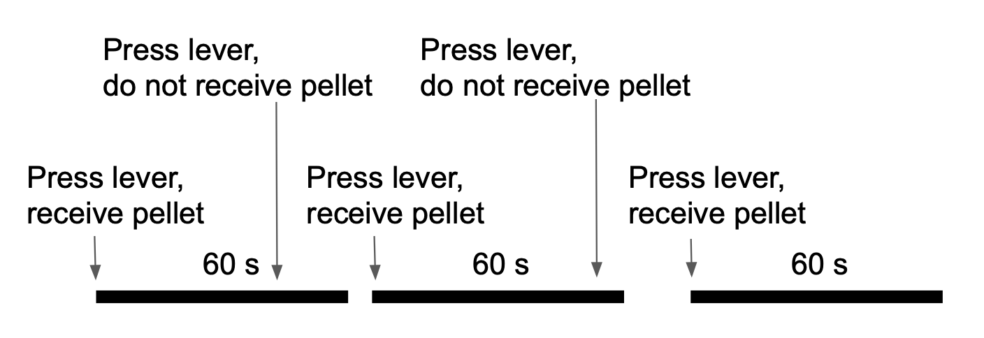
In toxicology, mice may be randomized to receive a particular dose of a toxicant and their subsequent actions measured (see, e.g., Ferster and Skinner (1957); Schneider (1969); Sobolewski et al. (2014); Eckard et al. (2023)). In a fixed interval experiment, which we analyze here, a mouse can take some action (e.g., pressing a lever), and in turn receive some reinforcer, such as a pellet of food. Receiving the food pellet begins a 60 s fixed interval, and if the mouse takes the action again before the fixed interval has elapsed, they receive no further reinforcer. However, if they take an action after the 60 s have elapsed, they receive another reinforcer, the reception of which begins the next fixed interval. In Figure 1, we show an example of three 60 s intervals in a fixed interval experiment, where the reinforcer is a food pellet and the action is the press of a lever. The fixed interval experiments we consider in this study occur within a “session” of length 30 minutes, so the mouse has a 30 minute block in which it can press as often as desired, receiving up to 30 food pellets and initiating up to 30 fixed intervals.
Usually, fixed interval experiments are analyzed by estimating the parameters that govern the animal’s behavior, where the animal’s behavior is reflected by the actions it takes. For example, one models the rate at which the animal pushes the lever (the action), with covariates corresponding to the different exposures (the states). In fact, this model is, for a conditional distribution of actions given states, called the “behavioral policy” in the reinforcement learning literature (Sutton and Barto, 2018). If we consider our outcome to be the summaries of the animal actions, such as the mean rate of lever presses, then modeling the behavioral policy is equivalent to an Analysis of Variance (ANOVA) (Scheffe, 1999), which is therefore commonly used for these types of experiments (often, a repeated measures ANOVA is used to assess behavior over time). An ANOVA might show that some toxicants increase a summary statistic of the animal’s response rate, as evidenced by a large coefficient on the exposure variable. Indeed, under certain exposures, such as 2,3,7,8-Tetrachlorodibenzodioxin (TCDD), mice show an inability to inhibit responding when working for the reinforcer, and might continue to press the lever many times before the 60 s has elapsed, even when receiving no food pellet (Sobolewski et al., 2014). A major difficulty, however, is in correctly specifying the model for the animal’s behavior. The mapping from exposure, which is often received in utero, to a mouse’s behavior is likely highly complex, and it is unlikely that the mapping from this exposure to the action in a complex behavioral experiment such as a fixed interval design corresponds to the model in an ANOVA. If the behavioral policy model proposed by the investigator is incorrect, the estimate that is obtained does not correspond to a true estimand reflecting the toxicant’s effect on the animal’s behavior.
The proposed approach, which we will now describe,allows us to sidestep having to specify the behavioral policy. Rather, we model the animal’s reward function. One can define a reward function for a mouse as a measure of the utility that the animal achieves after taking particular actions. For example, if the mouse times its presses well, it might receive 28 food pellets and only press once for each pellet, receiving many food pellets and also conserving energy. This will lead to a high reward. If a mouse however presses too frequently, it might also receive 28 food pellets, but it might expend more energy than necessary, leading to a low reward. Also, a mouse might conserve energy, only pressing a few times, but it might only receive a few food pellets, leading to a low reward overall. One can formally imagine a reward as a “function” of the animal’s actions, the number of food pellets received in a session, and the number of calories expended. Such a reward is generally as difficult or more difficult to specify than a behavioral policy, but, in this work, we do not model the reward directly.
Our work centers around the idea that the scientist who designed the fixed interval experiment has knowledge about what constitutes “optimal” behavior. For example, in the experiment described above, the experimenter knows that it is better for the mouse to wait and press the lever after 60 s rather than to expend energy with futile presses before the 60 s have elapsed. Sometimes, investigators see recurring, sophisticated optimal behaviors, such as scalloping, in which the animal’s response rates ramp up around the end of the fixed interval (Skinner, 1938). Because the experimenter might have a sense, often based on observed behavior of mice during their terminal sessions, of what the optimal action is, we can avoid specifying the reward function directly, and instead define a reward function in terms of the divergence from this proposed optimality. The tolerance for divergence from optimality then serves as a novel summary statistic, which can be derived for the exposed and unexposed mice (or for each dose of the exposure) and then serves as a novel summary of the effect of the exposure. Modeling the tolerance for divergence from optimality only requires choosing a way to quantify the divergence. More importantly, the estimand in our case is always well defined as a tolerance for divergence from optimality, whereas in the case of a misspecified behavioral policy, the estimand of the specified model may not correspond to any true estimand. Further, in the proposed framework, one can represent the mouse’s action and optimality in arbitrarily complex ways, allowing one to model complex experiments and incorporate sophisticated definitions of optimality. Finally, the proposed estimand is a scalar, and the objective function and framework are completely parametric, allowing one to use parametric theory to prove properties such as consistency, while still making very few assumptions about the nature of the distributions involved.
There is a rich body of work on modeling the timing of the animal’s lever presses in fixed interval experiments (Gibbon, 1977; Machado, 1997). Although these approaches provide interesting internal models of animal behavior, they do not cast it within a decision-theoretic, reinforcement learning framework. Our proposed approach falls in line with a body of literature on using the reinforcement learning framework to model behavior (Niv, 2009). In particular, our method is a novel approach to inverse-reinforcement learning (Russell, 1998), a growing research area in which one attempts to learn a reward function from data. Although there has been some activity on analyzing behavioral experiments in an inverse reinforcement-learning framework (Schultheis et al., 2021; Ashwood et al., 2022), our approach is the first to integrate into this endeavor an assessment of deviations from what the experimenter believes to be the optimal behavior. Designs for fixed interval experiment vary widely. We show how our method is useful for the standard fixed interval design, but it may apply equally well to other variations of these studies. Further, the idea of learning a reward that is a divergence from optimality can be quite general, and may apply to other more complex experiments, such as intermittent reinforcement designs.
3 Existing approach
Let the random variable denote the mouse’s exposure, where if the mouse was exposed to a toxicant and 0 otherwise. We also introduce the random variable for the mouse’s action, which could be, for example, the number of presses the animal makes per session in the experiment shown in Figure 1 (hence might be a summary statistic of the animal’s actions over time). Some true model, (where the subscript indicates that it is the true model), governs the animal’s actions given their exposures, which is, in a reinforcement learning framework, the mouse’s true “behavioral policy” (Sutton and Barto, 2018). It is common in these types of fixed interval experiments to specify a model, (where the subscript indicates that it is a specified behavioral model), for the true behavioral policy, as, for example,
| (1) |
which is not unreasonable for certain actions. Note that the model in (1) can arise in indirect ways; even a reasonable procedure, such as comparing averages over groups, is equivalent to assuming (1) as a model of the mouse’s policy. The model in (1) is equivalent to an Analysis of Variance (ANOVA) (Scheffe, 1999), and indeed the ANOVA approach is commonly used for the analysis of fixed interval experiments. However, specification of a behavioral policy that matches the true density, is quite difficult in practice. The true conditional density could be, in general, a highly complex function, and the space of possible choices for a model, for is vast. The model for the behavioral policy, is therefore likely to be misspecified. For example, even though it is a saturated model, a linear ANOVA model breaks down if the action is nonnegative, as is the case in many fixed interval experiments, since the number of presses in the session is the response variable. A log linear model might be more appropriate, but so might a Gamma distribution, for example. It is difficult to know which one to choose. In the simulations, we will show a case in which the true generating behavioral distribution is a complex Gamma distribution, and therefore it is quite different from a linear ANOVA, a log linear model, or anything that is possible to correctly specify.
Note that although, as mentioned, it is difficult to know whether an ANOVA is the correct model, using an ANOVA (or just comparing average behaviors over groups) is a reasonable choice for this type of experiment. Further, scientists often use a battery of measures to characterize a mouse’s behavior, and ANOVA is just one component of this. However, in this work, we seek to give an alternative to the ANOVA, which can possibly be used in conjunction with an ANOVA and other measures, enriching the overall analysis of the experimenter.
4 Methodology: optimality based-reward learning
Because of the difficulty in specifying the model for the true behavioral policy, we choose to avoid modeling it altogether. We instead model the mouse’s reward function. A reward function, like the behavioral policy, can be difficult to specify. However, we sidestep the need to specify the reward function by incorporating knowledge of the optimal behavior, which is known to the experimenter. We parameterize the reward, and, in learning this parameter, obtain a novel summary of the alteration caused by the toxicant.
4.1 Reward as divergence from optimality
Modeling a reward function is often more difficult than modeling a behavioral policy. However, we include in our reward function information known to the experimenter about optimality, which considerably simplifies the task. In other words, in a typical fixed interval experiment, such as the one shown in Figure 1, we can establish the optimal action, based on our understanding of the experiment. For example, in the experiment mentioned in Figure 1, one might expect near-optimal mice to allocate responses in a scallop pattern, in which they rarely press the lever right after receiving a food pellet, and then slowly increase their responses as the 60 s mark, which ends the fixed interval and portends a new food pellet, approaches (Skinner, 1938). For define Let denote the optimal action. For a particular mouse taking action , we can define a reward that penalizes divergence from optimality as
| (2) |
We negate the divergence, so a mouse will achieve the highest reward if it takes the optimal action, Note that this is an objective reward. In other words, if mouse 1 takes action , which is 1 unit away from the optimal action, and mouse 2 takes action which is 2 units away from the optimal action, then, according to (2), mouse 1 has a higher objective reward than mouse 2; i.e., .
4.2 A parameterized, subjective reward
Now, let us consider a definition of a personal, subjective reward, in which we will introduce a parameter, , which is specific to a particular type of mouse (e.g., mice that are exposed to a toxicant). Concretely, a subjective reward can be written, for specific to a mouse that takes action , as
| (3) |
Now, depending on this reward may not correspond to the objective reward in (2). Suppose again we have mouse 1 who is 1 unit away from the optimal action, and mouse 2 who is 2 units away from the optimal action. Suppose that mouse 1 belongs to a group with and mouse 2 belongs to a group with Then these two mice have equal subjective rewards, even though, as we saw before, their objective rewards differ: . In general, mice that diverge from the optimal action have a low reward. If a mouse never gets tired and also receives no benefit from the food pellet, it might have which implies that its action does not affect its reward.
4.3 Equality of subjective rewards
We assume that every animal in a fixed interval experiment takes actions that maximize their personal, subjective reward, as defined in Equation (3). We make the following remark, which is essential to performing estimation.
Remark 1.
Any two animals will have equal subjective rewards, since the animal with the lower reward can change their actions if this is not the case.
One can see the implications of Remark 1 by examining the reward function. In particular, for mouse from the exposed group E (with parameter ) taking action and for mouse from the control group C (with parameter ) taking action , we have that This only occurs if, using the definition of , Therefore, we are stating in Remark 1 that if mouse diverges more from the optimal action than mouse , then mouse tolerates divergence from optimality more than mouse , or that .
4.4 Identifying exposure-specific parameters
Now, let us create two groups corresponding to the exposed, and control, mice, indexed by or respectively. The parameter the exposed mouse’s true tolerance for divergence from optimality, or the alteration caused by the toxicant, is the estimand of interest in this work. The closer is to zero, the more the exposed animals tolerate a divergence from optimality relative to the controls. As discussed in Appendix A.1, the parameter is not identifiable (if we were to construct a system of equations using the form of in (3), the solution for will always be in terms of ). Let us impose the following constraint, which identifies ,
| (4) |
The constraint (4) allows us to rewrite the subjective reward in (3) as a function of the exposure,
| (5) |
Under (4.4), a mouse who was exposed has and, therefore, and a mouse who is a control has and, therefore,
4.5 Interpreting the estimand
Under the constraint in (4), any tolerance of divergence in the exposed group is associated with a corresponding lack thereof in the control group. Note that only if in which case both groups tolerate a divergence from optimality equally. If then the exposed mouse tolerates divergence from optimality more than the control mouse; i.e., the exposure is a toxicant. If then the exposed mouse tolerates divergence from optimality less than the control mouse; i.e., the exposure is beneficial (e.g., a medicine or essential nutrient).
4.6 Estimation
Now that we have, in (4.4), a parameterized model for the subjective, exposure-specific reward of any mouse, we can use it to find an estimator, for Note that we subscript our estimands by 0 and our estimators by To estimate , we rely on Remark 1, which states that any two animals will have the same subjective reward. We assume that any difference between subjective rewards in the observed animals whether they are exposed or not is, therefore, due to noise.
We can construct an objective function that represents the difference between subjective rewards for all pairs of mice in the experiment. Concretely, if we have observed independent and identically distributed state-action pairs, each corresponding to one mouse in a fixed interval experiment, we can compare each mouse with all the other mice,
| (6) |
Note that each mouse is compared to all other mice, regardless of group membership, but, within a group, the mice are constrained to have equal , and, hence, the out of group comparisons drive the differences in during estimation. Note that, based on (4.4), when depends on whereas when depends on but we only have to estimate because of the constraint in (4). One can find that makes these pairwise differences as small as possible, which aligns with Remark 1. Doing so drives to be small (or the tolerance for divergence to be large) for mice that act suboptimally, and vice versa for mice that act optimally. We then have an estimator for
| (7) |
5 Theory
We will now discuss some of the theoretical properties of our objective function in (6) and our estimator, We appreciated personal correspondence with Huber (2022), which keyed us in to the following remark.
Remark 2.
We have that the objective function in Equation (6) is equal to two times the sampling variance, i.e.,
For a proof, see Appendix A.2. Hence, finding a parameter that makes the subjective rewards of any two observed mice as close as possible is equivalent to finding a parameter that minimizes the empirical variance of the subjective rewards. Remark 2 is interesting in its own right, and it will also help us in the theory that follows. First, we will consider consistency of the proposed objective function.
Theorem 1.
The estimator is consistent for , where and is the population variance.
For a proof, see Appendix A.3.
One can also examine the rate of convergence of the objective function.
Theorem 2.
We have that
For a proof, see Appendix A.4.
We finally establish consistency of in the following theorem.
Theorem 3.
Assume that in practice only attains observed realizations, that are bounded; i.e., for all . We then have consistency of or that
For a proof, see Appendix A.5.
Since our estimator is a finite-dimensional minimum of an objective function, we have obtained consistency fairly easily. Note as well that this applies to arbitrarily complex actions; as long as its divergence from the optimal action is bounded, can be a vector (e.g., for time-dependent experiments), a matrix (e.g., for time-dependent experiments with grouped experimental units), or even a tensor.
6 Simulations
Suppose the true behavioral policy, that governs the animal’s actions , as a function of the exposure, is a distribution that is difficult to specify, such as a Gamma distribution () whose shape depends on in a complex way. For example, suppose the true, data-generating policy is
| (8) |
where and This model leads to larger or more activity, when on average; in summary, this model states that exposure causes hyperactivity in a complex way. Note that the true behavioral policy in (8) is unknown to the experimenter. The experimenter may model the behavioral policy nevertheless using (1), as is commonly done, or they may use the proposed method by optimizing (7). Set the sample size to be (this is small, which is reflective of the sample size in true fixed interval mouse experiments) and the number of Monte-Carlo datasets to be . We compare results when one fits a linear model to this data (i.e., (1)) to obtain an estimate of the exposure effect, to results when one uses the proposed method to optimize (7) for , shown in Figure 2. The exposure assignment, , is drawn randomly with probability 0.5.
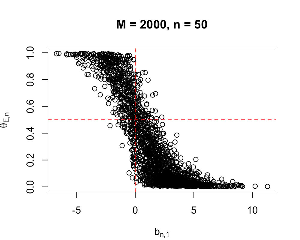
This is a very small sample of noisy data, but we see in Figure 2 that is often greater than zero, indicating that the exposure increases activity. This is accurate based on the model (the model in (8) leads to higher activity when on average). However, the parameter in the misspecified model does not correspond to the target estimands in the true model, in (8), which are , , . Yet, our estimate of which, when less than indicates that the exposure increases activity (by the discussion in Section 4.5), usually agrees (as shown in Figure 2) with in that is usually less than 0.5, also indicating that exposure increases activity. Although and usually, in a broad sense, come to the same conclusion about whether the exposure harms or benefits the mice ( for 73.85% of the simulated datasets and for 74.15% of the simulated datasets), the proposed method makes no assumption about the form of the behavioral policy in (8), and thus, in general, it is more robust. Further, the magnitude of and have different interpretations. Unlike does correspond to a true estimand and does have a valid interpretation as the tolerance for diverging from optimality in the exposed mice. The magnitude of is meaningful, whereas the magnitude of is only meaningful under correct specification of (1). Note that if we knew that the true model for was (1), it would be better to estimate However, we would not know this in practice.
In conclusion, we see that the estimate does not correspond to any estimand in (equation (8)), whereas the estimate corresponds to the exposed group’s tolerance for divergence from optimality, regardless of the true behavioral model .
7 Real Data analysis
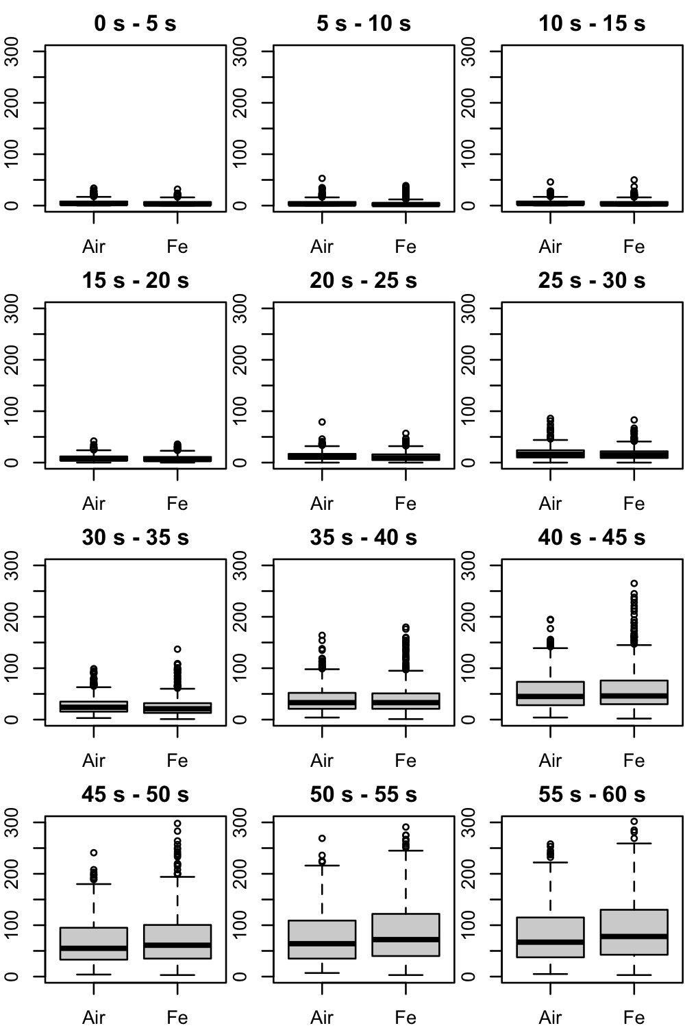
We analyze data from a fixed interval experiment in which mice are exposed to ambient iron (Eckard et al., 2023), which acts as a cerebral neurotoxicant. The fixed interval length was 60 s. Since the session is of length 30 minutes, a mouse can obtain up to 30 food pellets in one session. The sessions are performed times (and the mice tend to improve with each session). We show histograms for the number of presses in each 5 second time bin (over all sessions) in Figure 3. We observe that the iron-exposed mice are generally more hyperactive than the air-exposed (control) mice, and that both groups show an increase in their responses over time (a scallop pattern).
First, we describe how we define the actions of the mice. In the data from Eckard et al. (2023), we observed, for mouse within a session a vector of length 12,
where is the number of lever presses that occurred from seconds to seconds by mouse during session . We average over the sessions. Hence, we define the action for mouse averaged over sessions, as
Note that the action is a vector instead of scalar, as in the simulations. The flexibility with which one can represent the action is a strength of the proposed method. Conversely, if one models the same data using the approach in (1), one must first summarize (assuming one does not wish to employ complex, time-varying response models) the vector , with component defined as as , and then model
| (9) |
Let the bin midpoint times be defined as
Let the optimal action, a vector of length 12, be the strategy in which one makes only one press during the 0-5 second interval. Note that the initial lever press in a session starts a 60 second refractory interval; any press during this refractory interval does not yield a food pellet. A press is followed by receipt of a food pellet only if it occurs after this 60 second refractory interval has ended. The lever press that results in a food pellet initiates a new 60 session interval with the same constraints (Eckard et al., 2023). Hence, the optimal action, , is to press in the bin. If a mouse instead presses later in the interval, the pauses can add up so that a mouse might not receive the maximum number of food pellets in a session, which lasts exactly 30 minutes.
Although is optimal, it is not attainable by a mouse unless the mouse can be sure when the 0-5 second interval occurs (i.e., if the mouse has a stopwatch), so we do not measure the divergence from , but from a scaled version of it; i.e., we define the reward for mouse as
This reward forgives the first press and promotes a non-hyperactive scallop pattern (for more on the scallop, see e.g. Dews (1978); Skinner (1938)), which would be an optimal action for a mouse without a stopwatch or others means of knowing the time exactly.
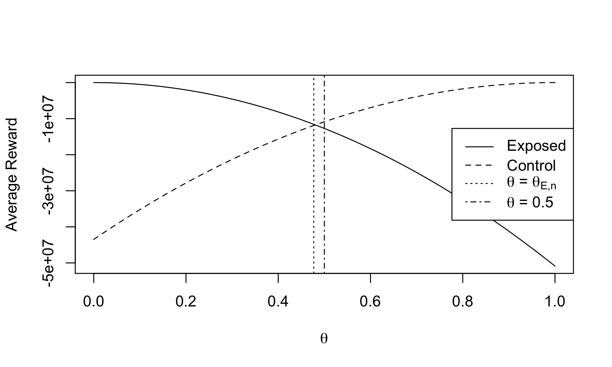
Given our definition for we finally optimize (7) to obtain estimate which implies that ambient iron alters the reward function of the mice, promoting suboptimal behavior. Conversely, using the ANOVA specified in (9), one obtains As discussed, if the true behavioral model is not correctly specified in (9), , unlike , will not correspond to a true estimand. In Figure 4, we include a visualization of the average reward (defined in (4.4)) for the exposed and control mice as a function of . Note that the average rewards are approximately equal at (note that (6) requires equality for the rewards of each animal rather than equality of the averages of the rewards, so is not exactly where the curves cross, but it is very close). We see that As discussed in Section 4.5, this implies that the exposed mice tolerate divergence from optimality more than the control mice.
8 Discussion
We have proposed a method for analyzing a fixed interval experiment that sidesteps the difficulties associated with specifying a behavioral policy, or a conditional density of actions given exposures, by instead modeling the animal’s reward function. The proposed method also sidesteps the need to specify a reward function explicitly by incorporating knowledge known to the experimenter on optimality. The parameters of the reward function are finite-dimensional, but make very few assumptions about the data generation itself. Ultimately, better analysis of fixed interval experiments allows us to better utilize resources when designing these experiments and potentially to better understand the effects of toxicants that are present in our environment, which is a necessary step toward protecting humans from exposure.
We first discuss some limitations and future directions of the real data analysis. In this study, we analyze the animal behavior averaged over all the sessions. However, the “scallop” behavioral pattern should improve for each animal as the sessions progress. Future analysis might consider computing the estimator as it changes over sessions, which would correspond to the animal’s behavior approaching the behavioral optimality over time, which could then further be assessed as it differs between the control and exposed mice. Note also that the bins are 5 seconds long in this study. Changing the bin size might change results. Ideally, if one knew the time of each press, one could adapt the proposed method to penalize the deviation of each press from optimality, rather than averaging over all presses within a given bin and computing the deviation of this average from optimality, as we have done here. Finally, the data is collected in a free operant system; i.e., the animals can skip intervals early on in training. To better quantify the scallop, one could use a system with discrete operant trials; i.e., one could give animals an inter-trial interval time, where the lights go off to signal that the 60 second interval is over and then go back on to start another interval. The skipping of intervals creates noise in the analysis. The skipping is mostly a problem during early sessions, before the animals have adequately learned the task. One could potentially assess the degree to which animals skip reinforcers in the early sessions, and one could eliminate early sessions from the analysis, if needed. Alternatively, one could use an norm in (3), which is more robust to noise created by skipping. Another interesting direction might be to develop a version of the metric that conditions on more information, in the form of covariates. The estimator we provide marginalizes over these covariates, but a conditional model might be of scientific interest to provide a more subject-specific analysis.
We now discuss some limitations of the proposed method. When defining the reward under our proposed method, we do have to choose a metric, such as an or norm, for the distance between the observed and optimal actions. The choice of norm, however, is not an assumption in the way that a specific model for is an assumption. In other words, if we choose an norm, our conclusions are that the tolerance for norm divergence from the optimal is estimated by but if we choose the norm, our conclusion is that the tolerance for norm divergence from the optimal is both of these can be true statements, since the magnitude of does not have any intrinsic meaning. However, if we misspecify a model for a statement that corresponds to some estimand in which is what underlies the assumption that is our chosen model, is false. Note also that in the proposed approach we are choosing to focus only on divergence from optimality rather than on the direction of divergence. By providing a sign on the coefficient, an ANOVA does provide a sort of inference for the sign of the effect of the toxicant (whether the toxicant increases of decreases actions). However, the correctness of the ANOVA coefficient sign is dependent upon the correct specification of the ANOVA. One could glean a rough estimate of the sign of the effect in our case by taking a contrast of the exposed and control group average actions. In general, however, in many toxicological experiments, it may be useful to establish whether there is an effect at all at a certain exposure level and dose, a fact that can be then augmented by an understanding of the biological mechanism of the effect to determine the likely direction of the effect and implications for those who are exposed.
One additional contribution of our work here is to fully cast the fixed interval mouse experiment within a reinforcement learning framework. When viewing a fixed interval experiment in a reinforcement learning framework, other possible statistical summaries besides the proposed also come to mind. Some might be quite useful, and they are discussed in terms of their relationship with in Appendix A.6. However, has certain favorable properties. For example, the magnitude of is bounded in the range regardless of the scale of which cannot be said for other more ad-hoc statistics. Further, is the solution to an optimization problem, and, besides giving the statistic concrete meaning (although the magnitude of the statistic does not have inherent meaning, it can be interpreted as a tolerance for divergence, which is higher when it is near zero), this optimization allows one can to use results such as those shown in Theorems 1 and 2 to ultimately draw conclusions on the consistency of in Theorem 3. Further, although the statistic requires very few assumptions, it is still parametric, and therefore will have favorable convergence properties. In general, with other methods, it is difficult to obtain the combination of a small number of assumptions, the benefits of a parametric model, and the underlying optimization framework that are jointly offered by . It is difficult to interpret behavior from any one summary variable, so scientists use behavioral batteries in multiple domains, and look for broad patterns. We hope that the proposed statistic provides a new addition to these batteries.
9 Acknowledgements
This work is solely the responsibility of the authors and not the funding agencies. Research reported in this publication was supported by the National Institutes of Health (NIH) under award numbers T32ES007271 (National Institute of Environmental Health Sciences (NIEHS)) and T32GM007356 (National Institute of General Medical Sciences (NIGMS)).
Appendix A Appendix
A.1 Identifiability
Consider the population exposed mouse and population control mouse, who take actions We are claiming that their subjective rewards are equal, or that
| (10) |
We will now give a small example showing non-identifiability without the constraint in (4), which was . Suppose We will start with (10) and show that, under these conditions, we have more than one solution for Assume no constraint on and and write, using the definition of in (3),
| (11) |
Hence, for we obtain and for we obtain and both imply (10), implying a lack of identifiability. When we impose identifiability constraint from (4). Starting from (A.1), we have uniqueness of
A.2 Proof of Remark 2
Proof.
A.3 Proof of Theorem 1
A.4 Proof of Theorem 2
Proof.
Start with (A.2) derived in the proof of Remark 2, or that
Multiply through by to obtain
Note that and both are scaled averages of iid variables and, therefore, converge in distribution to normal random variables by the Central Limit Theorem. Hence, and are The term the product of a normally distributed random variable and an average that converges to zero, disappears by Slutsky’s theorem. ∎
A.5 Proof of Theorem 3
Proof.
By the algebra shown in the proof of Theorem 1, we have that our objective function in (7) is just two times the sample variance, Note that therefore
and
Note that is continuous in differentiable, and has a unique minimum at Hence, by theory on the consistency of extremum estimators (Amemiya, 1985), if we can show that converges uniformly in probability to , we have that
We must show that is Lipschitz. This, in conjunction with the facts that (1) is in a compact set and (2) we have pointwise convergence in probability, , would allow us to conclude, by Theorem 1, that we have, by Newey (1991), uniform convergence in probability of to .
Hence, we need only to show that is Lipschitz. By the Mean Value Theorem, we can show that a function is Lipschitz by showing that its first derivative is bounded. We therefore examine the derivative of below. Note that
We need to show that the derivative of the preceding display is bounded, which occurs if the derivatives of the summands are bounded. Differentiating the summand with respect to we obtain
which is bounded as long as is bounded, which holds by assumption. Since the derivative of is bounded, we have that is Lipschitz. By the preceding discussion, we therefore have that
∎
A.6 Other statistical summaries
One might also consider comparing the average divergence from optimality for each group as
where are the indices of all exposed mice and vice versa for This statistic depends on two statistics that use only half of the observations each, whereas is estimated using all observations. Further, the magnitude of this statistic will depend on the scales of and whereas for any problem. One might consider normalizing somehow, but these types of manipulations become ad-hoc. Also, the lack of an optimization objective makes it difficult to see what the statistic means in terms of the exposure, whereas with , it is clear: is the exposed animal’s tolerance for divergence from optimality, as it relates to the control, and it is the only statistic that solves the optimization in (7). Another statistic that does not require specification of the behavioral policy would just be a Wilcoxon test for the actions in the two groups, and although this does not assume a model, it is nonparametric, whereas our approach is still parametric, facilitating consistency arguments such as the ones made in Theorem 3 even under mild assumptions on the nature of the action .
References
- Amemiya (1985) Takeshi Amemiya. Advanced econometrics. Harvard University Press, 1985.
- Ashwood et al. (2022) Zoe Ashwood, Aditi Jha, and Jonathan W. Pillow. Dynamic inverse reinforcement learning for characterizing animal behavior. In Alice H. Oh, Alekh Agarwal, Danielle Belgrave, and Kyunghyun Cho, editors, Advances in Neural Information Processing Systems, 2022. URL https://openreview.net/forum?id=nosngu5XwY9.
- Dews (1978) PB Dews. Studies on responding under fixed-interval schedules of reinforcement: Ii. the scalloped pattern of the cumulative record. Journal of the Experimental Analysis of Behavior, 29(1):67–75, 1978.
- Eckard et al. (2023) ML Eckard, E Marvin, K Conrad, G Oberdörster, M Sobolewski, and DA Cory-Slechta. Neonatal exposure to ultrafine iron but not combined iron and sulfur aerosols recapitulates air pollution-induced impulsivity in mice. NeuroToxicology, 94:191–205, 2023.
- Ferster and Skinner (1957) Charles B Ferster and Burrhus Frederic Skinner. Schedules of reinforcement. 1957.
- Gibbon (1977) John Gibbon. Scalar expectancy theory and weber’s law in animal timing. Psychological review, 84(3):279, 1977.
- Gilbert (2004) Steven G Gilbert. A small dose of toxicology: the health effects of common chemicals. CRC Press, 2004.
- Huber (2022) William Huber. Distribution of minimizer of sum of squared pairwise differences. Cross Validated, 2022. URL https://stats.stackexchange.com/q/579953. URL:https://stats.stackexchange.com/q/579953 (version: 2022-10-07).
- Machado (1997) Armando Machado. Learning the temporal dynamics of behavior. Psychological review, 104(2):241, 1997.
- Newey (1991) Whitney K Newey. Uniform convergence in probability and stochastic equicontinuity. Econometrica: Journal of the Econometric Society, pages 1161–1167, 1991.
- Niv (2009) Yael Niv. Reinforcement learning in the brain. Journal of Mathematical Psychology, 53(3):139–154, 2009.
- Russell (1998) Stuart Russell. Learning agents for uncertain environments. In Proceedings of the eleventh annual conference on Computational learning theory, pages 101–103, 1998.
- Scheffe (1999) Henry Scheffe. The analysis of variance, volume 72. John Wiley & Sons, 1999.
- Schneider (1969) Bruce A Schneider. A two-state analysis of fixed-interval responding in the pigeon 1. Journal of the Experimental Analysis of Behavior, 12(5):677–687, 1969.
- Schultheis et al. (2021) Matthias Schultheis, Dominik Straub, and Constantin A Rothkopf. Inverse optimal control adapted to the noise characteristics of the human sensorimotor system. Advances in Neural Information Processing Systems, 34:9429–9442, 2021.
- Skinner (1938) BF Skinner. The behavior of organisms: an experimental analysis. 1938.
- Sobolewski et al. (2014) Marissa Sobolewski, Katherine Conrad, Joshua L Allen, Hiromi Weston, Kyle Martin, B Paige Lawrence, and Deborah A Cory-Slechta. Sex-specific enhanced behavioral toxicity induced by maternal exposure to a mixture of low dose endocrine-disrupting chemicals. Neurotoxicology, 45:121–130, 2014.
- Sutton and Barto (2018) Richard S Sutton and Andrew G Barto. Reinforcement learning: An introduction. 2018.