Detecting Ultralight Dark Matter Gravitationally
with Laser Interferometers in Space

Abstract

Ultralight dark matter (ULDM) is one of the leading well-motivated dark matter candidates, predicted in many theories beyond the standard model of particle physics and cosmology. There have been increasing interests in searching for ULDM in physical and astronomical experiments, mostly assuming there are additional interactions other than gravity between ULDM and normal matter. Here we demonstrate that even if ULDM has only gravitational interaction, it shall induce gravitational perturbations in solar system that may be large enough to cause detectable signals in future gravitational-wave (GW) laser interferometers in space. We investigate the sensitivities of Michelson time-delay interferometer to ULDM of various spins, and show vector ULDM with mass $m\lesssim 10^{-18}~{}$eV can be probed by space-based GW detectors aiming at $\mu$Hz frequencies. Our findings exhibit that GW detectors may directly probe ULDM in some mass ranges that otherwise are challenging to examine.

Introduction.—Dark Matter (DM) constitutes the majority of matter in the universe, with supporting evidence from galactic rotational curves, bullet cluster, large-scale structure and cosmic microwave background. However, DM’s identity remains unclear because all the confirmed evidence merely suggests DM must have gravitational interaction. Among the leading candidates, ultralight dark matter (ULDM) with mass $\lesssim 10^{-6}~{}$eV stands out attractively since it may connect to fundamental physics at very high energy [1, 2, 3, 4, 5, 6], including quantum gravity [7, 8], grand unified theory [9, 10, 11], inflation [12, 13, 14, 15, 16], etc.

There have been vast efforts and significant progresses in searching for ULDM, either presuming there are additional nongravitational interactions between ULDM and normal matter [17, 18, 19] or just gravity. For instance, searching for axion-like ULDM [20, 21, 22] involves interactions with photon [23, 24, 25, 26, 27, 28], electron [29, 30, 31, 32], nucleon [33, 34, 35, 36, 37] or neutrino [38, 39, 40]. Dark photon ULDM searches assume its mixing with photon [41, 42, 43, 44, 45, 46, 47, 48, 49, 50]. After the detection of gravitational waves (GWs), it was shown that gravitational-wave (GW) experiments can also be very sensitive to some of such interactions [51, 52, 53, 54, 55].

Astrophysical methods that only employ ULDM’s gravitational interaction are also pushed forward, including probing metric perturbation by pulsar timing array (PTA) [56, 57, 58, 59, 60, 61, 62, 63, 64, 65, 66], binary dynamics [67, 68, 69, 70], Lyman-$\alpha$ constraints [71, 72, 73], 21cm absorption line [74, 75], superradiance around black holes [76, 77, 78, 79, 80, 81], and galactic dynamics [82, 83, 84, 85]. Such searches can provide complementary information and are largely model-independent unless non-gravitational interaction dramatically change the physical contexts.

In this work, we present the searches for local ULDM of various spins by space-based GW laser interferometers. Unlike the scalar case that suffers from velocity suppression, we demonstrate that the gravitational tensor perturbations in solar system caused by vector ULDM can lead to detectable signals, which may be probed by future GW laser inteferomerters in space with arm lengths comparable to the diameter of Mars’ orbit. Detection of such a signal would directly suggest the wave nature of DM and its mass range, signifying the fundamental theory of DM.

Metric perturbations and signal response.—Since we are considering the effects of ULDM in solar system at a time scale of years, we can neglect the cosmic expansion and write the metric with linear perturbations over a flat background, defining scalar metric perturbations $\Psi$ and $\Phi$, and tensor $h_{ij}$ by

$$ds^{2}=-(1+2\Psi)dt^{2}+[(1-2\Phi)\delta_{ij}+h_{ij}]dx^{i}dx^{j}.$$ (1)

In the Poisson gauge we have $\partial_{i}h_{ij}=\delta_{ij}h_{ij}=0$. The energy-momentum tensor $T_{\mu\nu}$ of ULDM would source metric perturbations through the Einstein equations. For ULDM with mass $m$, energy density $\rho$ and velocity $v$, we can estimate the amplitudes of perturbations,

$$\Psi^{j}\simeq\Phi^{j}\simeq\pi G\frac{\rho}{m^{2}}= \frac{7\times 10^{-26}\rho}{0.4\,\text{GeV/cm}^{3}}\left(\frac{10^{-18}\text{eV}}{m}\right)^{2},$$ (2)

$$h^{v}_{ij}\propto h_{0}\simeq\frac{8}{3}\pi G\frac{\rho}{m^{2}}= \frac{2\times 10^{-25}\rho}{0.4\,\text{GeV/cm}^{3}}\left(\frac{10^{-18}\text{eV}}{m}\right)^{2},$$ (3)

and $h^{s}_{ij}\simeq h_{0}v^{2}/2$. Here the superscript $j=s$ and $v$ stands for contribution from scalar and vector ULDM . Note that $h^{s}_{ij}$ due to scalar ULDM are suppressed by $v^{2}$ (see Supplemental Material). However, the tensor perturbation $h^{v}_{ij}$ for vector ULDM is not suppressed, which is crucial for the detection by interferometers in space.

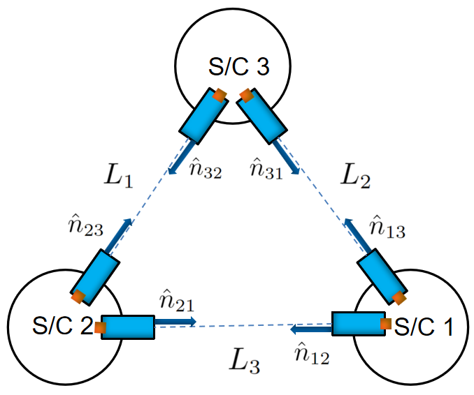
Figure 1: A Schematic of the triangle constellation for LISA-like GW laser interferometers in space. Each spacecraft (S/C) hosts two test masses (orange cubic) and each single-link measurement encodes the distance between two test masses at two ends of an edge. $\hat{n}_{ij}$ denotes the unit direction vector pointing from S/C $i$ to S/C $j$. The arm lengths $L_{i}$ are changing over time with percent-level variation.

Now we derive the signal response of a space-based GW interferometer to the metric perturbations sourced by ULDM. We consider the constellation with three spacecrafts (S/C) as Fig. 1, which is adopted in most space-based GW detectors, including LISA [87], Taiji [88], Tianqin [89], BBO [90], DECIGO [91], $\mu$Ares [92], LISAmax [93], and ASTROD-GW [94]. The signal is encoded in the fractional frequency shift,

$$y_{rs}(t)\equiv\frac{\delta\nu_{rs}(t)}{\nu_{0}}\simeq z_{\Phi}(t)+z_{h}(t)+N(t),$$ (4)

which parameterizes various effects on the single-link frequency shift $\delta\nu_{rs}$ of the transmitted laser light from S/C $s$ to S/C $r$, including instrumental noises $N(t)$ and geodesic deviations from perturbations $\Phi$ and $h_{ij}$, $z_{\Phi}(t)+z_{h}(t)$. The central laser frequency is taken as $\nu_{0}\simeq 2.81\times 10^{14}$ Hz as the wavelength of laser light is $1064$ nm.

Instrumental noises and TDI combinations.—Three main instrumental noises, contributing to $\delta\nu_{rs}(t)$, would limit the detection sensitivity, including frequency noise of lasers $p_{i}(t)$, acceleration noise of test masses $s_{\text{acc}}$, and noise of optical metrology system $s_{\text{oms}}$. Frequency noise is related to how monochromatic the laser light is, while acceleration noise denotes the deviation of free fall for test mass, and metrology noise represents the displacement uncertainty of optical interferometers.

Due to the mismatch of time-changing arm lengths, the laser frequency noise in a single-link data stream $y_{rs}(t)$, $p_{s}(t-L_{j})-p_{r}(t)$, does not cancel and dominates over all other ones by several orders. To suppress laser noise to a negligible level, the usual strategy is to postprocess the acquired data by time-delay interferometry (TDI) algorithm [95], which makes time-shifts and linear combinations of $y_{rs}(t)$, or equivalently constructs virtual equal-arm interferometry. One example for Michelson combination $X(t)$ can be written as follows,

$$X(t)=\big{[} y_{13}(t)+y_{31}(t-L_{2})+y_{12}(t-2L_{2})$$

$$+y_{21}(t-L_{3}-2L_{2})\big{]}-\big{[}y_{12}(t)+y_{21}(t-L_{3})$$

$$+y_{13}(t-2L_{3})+y_{31}(t-L_{2}-2L_{3})\big{]}.$$ (5)

The combinations in two brackets can be geometrically described in Fig. 2 by the blue and black light paths, respectively. Two paths have almost equal lengths, $2L_{2}+2L_{3}$, but in different directions, indicated by the arrows. Many other combinations are possible (see Supplemental Material). The laser frequency noise in such combinations can be suppressed and hence neglected in further discussions. Also $L_{i}$ appearing in all other contributions can be approximately taken as $L_{i}=L$, the nominal arm length of the triangle constellation.

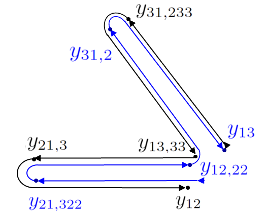
Figure 2: The schematic of Michelson combination $X$ centered at S/C 1. For time delays, we use the convention, $y_{ij,kl\cdots}=y_{ij}(t-L_{k}-L_{l}\cdots)$. The light paths of two colors are nearly equal so that laser frequency noise is effectively suppressed.

	LISA	Taiji	Tianqin	BBO	DECIGO	$\mu$Ares	LISAmax	ASTROD-GW
$L$ ($10^{9}$m)	$2.5$	$3$	$0.17$	$0.05$	$1\times 10^{-3}$	$395$	$260$	$260$
$s_{\text{acc}}$ ($10^{-15}\frac{\textrm{m/s}^{2}}{\sqrt{\textrm{Hz}}}$)	$3$	$3$	$1$	$3\times 10^{-2}$	$4\times 10^{-4}$	$1$	$3$	$3$
$s_{\text{oms}}$ ($10^{-12}\frac{\textrm{m}}{\sqrt{\textrm{Hz}}}$)	$15$	$8$	$1$	$1.4\times 10^{-5}$	$2\times 10^{-6}$	$50$	$15$	$100$
$\dfrac{\rho}{\rho_{0}}$($5.0\times 10^{-19}\text{eV}$)	$7.95\times 10^{2}$	$6.53\times 10^{2}$	$3.82\times 10^{3}$	$2.00\times 10^{2}$	$1.34\times 10^{2}$	$0.44$	$7.67$	$4.32$

Table 1: Arm lengths and instrumental noises of several planned laser interferometers in space. In the last row we give the sensitivities on vector ULDM with mass $5.0\times 10^{-19}\text{eV}$. Here $L$ is the nominal arm length of triangle constellation, while $s_{\text{acc}}$ and $s_{\text{oms}}$ are the acceleration noise of test mass and noise from optical metrology system, respectively. Note that LISA/LISAmax/Taiji/Tianqin adopt frequency-dependent noise power spectra [96], $s^{2}_{\text{acc}}\propto[1+\left(0.4\times 10^{-3}~{}\textrm{Hz}/f\right)^{2}][1+\left({f}/{8\times 10^{-3}~{}\textrm{Hz}}\right)^{4}]\;$ and $s^{2}_{\text{oms}}\propto 1+\left({2\times 10^{-3}~{}\textrm{Hz}}/{f}\right)^{4}$.

On the other hand, acceleration noise and metrology noise cannot be suppressed and consequently limit the detection sensitivity. In Table. 1, we list the noise power spectral density (PSD) for several future laser interferometors in space. To compare with the signal strain in $X$ directly, we calculate the noise power spectrum in Michelson combination, Eq. Detecting Ultralight Dark Matter Gravitationally with Laser Interferometers in Space,

$$N_{X}(\omega)=16\sin^{2}\omega L\left[2(1+\cos^{2}\omega L)\frac{s^{2}_{\text{acc}}}{\omega^{2}}+\omega^{2}s^{2}_{\text{oms}}\right],$$ (6)

where $\omega$ is the angular frequency and $\omega=2\pi f$. It is expected that acceleration noise would dominate at low frequencies due to the $\omega^{-2}$ factor while optical metrology noise dominates at high frequencies because of $\omega^{2}$ term. In the low-frequency limit, $\omega L\ll 1$, we have $N_{X}(\omega)\simeq 64L^{2}s^{2}_{\text{acc}}$, which is frequency-independent for constant $s_{\text{acc}}$. At first sight, it seems longer arms would make detectors less sensitive. However, as we shall shown, the signal PSD also depends on $L$ and eventually prefers larger arm lengths.

Sensitivities to ULDM.—To estimate the sensitivity of a laser interferometer to ULDM, we calculate the signal PSD of $X(t)$ in frequency domain, and compare it with the noise PSD, $N_{X}(\omega)$ in Eq. 6. The ULDM PSD of $X(t)$ in observation duration $T$ is related to the amplitude in frequency domain, $\tilde{X}(\omega)$,

$$S_{X}(\omega)=|\tilde{X}(\omega)|^{2}/T=S^{j}_{\Phi}+S^{j}_{h},$$ (7)

where we have separated the contributions from scalar and tensor metric perturbations into $S^{j}_{\Phi}$ and $S^{j}_{h}$, respectively, and performed the sky average over the propagation direction of ULDM, and additional average over the polarizations for vector ULDM. We have neglected the cross term $S_{\Phi h}$, which either vanishes after averaging over directions and polarizations, or is subdominant. Parameterizing ULDM as superpositions of plane waves with frequency dispersion $\delta\omega\sim mv^{2}$, we observe that $S_{X}(\omega)$ has a nearly monochromatic component at $\omega=2m$ .

Specifically, for ULDM propagating along some direction $\hat{k}=\vec{k}/|\vec{k}|(\vec{k}=m\vec{v})$, we have

$$S^{j}_{\Phi}(\hat{k}) \simeq v^{2}_{\text{osc}}T\Big{|}\hat{k}\cdot\hat{n}_{13}\big{[}1-e^{-i8mL}-2e^{-i(2mL+2\vec{k}\cdot\hat{n}_{13}L)}$$

$$+2e^{-i(6mL+2\vec{k}\cdot\hat{n}_{13}L)}\big{]}-\hat{k}\cdot\hat{n}_{12}\big{[}1-e^{-i8mL}$$

$$-2e^{-i(2mL+2\vec{k}\cdot\hat{n}_{12}L)}+2e^{-i(6mL+2\vec{k}\cdot\hat{n}_{12}L)}\big{]}\Big{|}^{2},$$ (8)

where $v_{\text{osc}}=\kappa^{2}\rho v/4m^{2}$, $\kappa\simeq\sqrt{4\pi G}$. And

$$S^{s}_{h}(\epsilon_{ij})\simeq\frac{64}{9}\kappa^{4}\rho^{2}v^{4}L^{4}T[(\hat{n}_{12}^{i}\hat{n}_{12}^{j}-\hat{n}_{13}^{i}\hat{n}_{13}^{j})\epsilon_{ij}]^{2},$$ (9)

where $\epsilon_{ij}$ is the polarization tensor and should be averaged in later numerical evaluations. A quick estimation shows the average of the term in bracket gives an $\mathcal{O}(1)$ factor.

Under the low-frequency approximation, $mL\ll 1$, we average the propagation direction $\hat{k}$ analytically,

$$S^{s}_{\Phi}\simeq\frac{64}{15}\kappa^{4}\rho^{2}v^{2}L^{4}T\;\left[v^{2}\sin^{2}\gamma+5m^{2}L^{2}\sin^{2}\frac{\gamma}{2}\right],$$ (10)

where $\gamma$ is the angle between two arms of the triangle, $\gamma\simeq\pi/3$. When $mL\gg v^{2}\simeq 10^{-6}$, the second term in bracket would be dominant and $S^{s}_{\Phi}\propto m^{2}v^{2}L^{6}$. Otherwise, $S^{s}_{\Phi}\propto v^{4}L^{4}$ and comparable to $S^{s}_{h}$. In both cases, longer arms give larger signal PSD.

However, for vector ULDM the dominant contribution comes from the tensor perturbation,

$$S^{v}_{h}(\epsilon_{ij})\simeq\frac{256}{9}\kappa^{4}\rho^{2}L^{4}T[(\hat{n}_{12}^{i}\hat{n}_{12}^{j}-\hat{n}_{13}^{i}\hat{n}_{13}^{j})\epsilon_{ij}]^{2}.$$ (11)

Note that $S^{v}_{h}$ is significantly larger than $S^{v}_{\Phi}$, at least by a factor of $1/v^{2}\sim 10^{6}$. Therefore $S^{v}_{\Phi}$ can be neglected.

It is now evident that larger arm length $L$ gives larger power spectrum $S_{X}$, which suggests that at the same noise level GW detectors in space with longer arms would have better sensitivity to ULDM. To estimate the sensitivity quantitatively, we define it as the value of density $\rho$ with which the signal-to-noise ratio (SNR) reaches unity,

$$\text{SNR}=\frac{S_{X}(\omega)}{N_{X}(\omega)}=1.$$ (12)

At low frequencies we have $\rho\propto\kappa^{2}s_{\text{acc}}/L\sqrt{T}$. When the sensitivity $\rho$ of some detector is less than or equal to DM’s local density $\rho_{0}\simeq 0.4~{}\text{GeV/cm}^{3}$, namely $\rho/\rho_{0}\lesssim 1$, such a detector would be able to probe local ULDM in solar system.

In Fig. 3 we plot the sensitivities of various GW detectors to scalar and vector ULDM. For scalar ULDM, the most sensitive range is around $m\sim 10^{-18}$ eV by $\mu$Ares [92], which is aiming at detecting $\mu$Hz GWs. The sensitivity surpasses that from planetary ephemerides in solar system [67], reaching $\rho/\rho_{0}\sim 10^{3}$. This large value also suggests that, unless there are huge improvements on instrumental noises by several orders of magnitude or there are DM clumps near solar system, it is difficult to probe local scalar ULDM gravitationally through GW detectors in space.

Interestingly, for vector ULDM with $m\lesssim 10^{-18}$ eV $\mu$Ares is able to probe $\rho/\rho_{0}\simeq 0.4$, indicating the possibility to detect local DM gravitationally. In this case, at low frequencies the flat behaviour of sensitivities from $\mu$Ares, ASTROD-GW, DECIGO and BBO as well, results from the frequency independence of $N_{X}(\omega)$ and $S_{h}$ when $\omega L\ll 1$. For LISA, Taiji, Tianqin and LISAmax, the adopted acceleration noises $s_{\text{acc}}$ have non-trivial frequency dependence, making them less sensitive at lower frequencies. The plot demonstrates that at low frequencies the sensitivity goes as $\rho\propto L^{-1}$, which is quite different from the scalar ULDM case where $\rho\propto L^{-2}$ for $1\gg mL\gg v^{2}\sim 10^{-6}$, indicated by Eq. 10. It also exhibits that all discussed GW detectors in space would surpass planetary ephemerides in some mass ranges. These findings extends the scientific objects for future GW detectors in space.

We have conducted the above numerical analysis by employing the first-generation time-delay interferometry (TDI), which assumes static arm lengths. However, the sensitivities and conclusions do not change if we use the second-generation TDI with time-changing arm lengths, which doubles the terms in $X(t)$ and the light paths in Fig. 2. The resulting noise and signal PSDs would be modified by the same factor $4\sin^{2}(2mL)$ and cancel out in the signal-to-noise ratio. Furthermore, we have only used the Michelson channel. Many other channels are possible, which can provide additional information of the signal, like the spin of ULDM (Supplemental material).

For comparison, we show the inferred limit from the GRACE-FO satellite project [98], which has validated the laser metrology to be deployed in LISA. There are only two spacecrafts in GRACE-FO whose separation is monitored by laser interferometers. Although not capable to detect GW or ULDM, the overall noise level in the collected data can still give a constraint, shown as the pink curve in the upper plot. Similar to GWs, the tensor metric perturbation induced by ULDM also leads to a distortion of the apparent angular positions of stars, a rough estimation for its detectability with Gaia-like astrometric accuracy (see Supplemental Material) is shown in the lower plot. Both limits are considerably weaker than that from planetary ephemerides, and GW detectors in space.

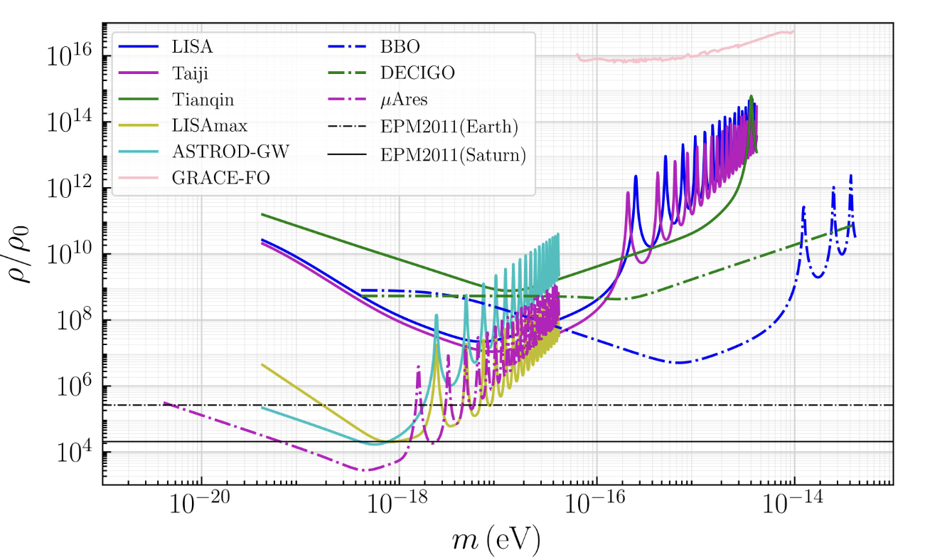
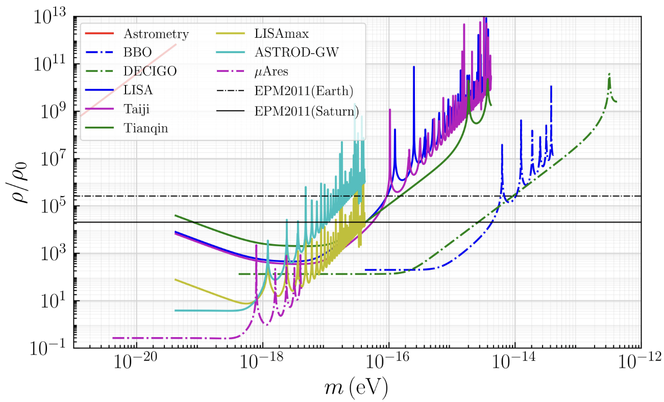
Figure 3: (Upper) Sensitivities to $\rho$ for scalar ULDM. (Lower) Sensitivities to $\rho$ for vector ULDM. We assume one-year observation time for LISA, Taiji, Tianqin, BBO, DECIGO, LISAmax and ASTROD-GW, ten years for $\mu$Ares and 13 days for GRACE-FO (pink curve). For comparison, we also show the constraints (horizontal lines) derived from the solar system planetary ephemerides [67] and the estimated astrometric detection threshold (the red line in lower panel).

Conclusion and Outlook.—We have elucidated that future space-based GW laser interferometers can provide new insights into detecting ULDM and extend the scientific objectives. Without assuming any additional interactions between ULDM and normal matter, the gravitational perturbations caused by vector ULDM with mass $m\lesssim 10^{-18}~{}$eV in solar system is able to perturb the geodesics of test masses at a detectable level if the arm length of the triangle constellation is comparable to the diameter of Mars’ orbit. For scalar ULDM, although not capable to make a detection, GW detectors would probe the mass range around $10^{-18}~{}$eV that other experiments are challenge to explore. This investigation highlights the unique advantage of GW detectors in space. Detection of such a signal would directly suggest the wave nature of DM and its mass and spin, indicating the fundamental theories of DM.

To distinguish the ULDM signal from GW events from compact binaries nearby galaxies, it is necessary to go beyond the power spectral density and perform matched filtering in time domain or even joint observation with multiple detectors. A more sophisticated treatment would be comparing the outcome of various TDI combinations, which at low frequencies have different sensitivities to ULDM of different spins and GWs. The anisotropic distribution of such GWs would also be distinct. Dedicated investigations are warranted in future work.

Supplementary Material for Detecting ULDM with Laser Interferometers in Space
Jiang-Chuan Yu, Yan Cao, Yong Tang, and Yue-Liang Wu

This Supplementary Material contains supporting analysis, formulas and figures for the main letter. In Sec. I, we show the specific form of metric perturbations induced by scalar and vector ULDM. In Sec. II, we present the single-link laser signal of purely gravitational ultralight DM fields for space-based interferometers. We find that the signal consists of three kinds of components, namely the frequency shift of the photons induced by scalar and tensor metric perturbations and the motions of test-masses. Then in Sec. III we derive the signal power spectrum and projective sensitivities of various space-based GW interferometers to the local ULDM for TDI-X channel and compare the responses of various TDI combinations. Finally, we show the DM signals given by other experiments in Sec. IV, especially other laser interferometers in space and astrometric effects.

I Metric perturbations from ultralight dark matter

In this section, we review the metric perturbations sourced by nonrelativistic ULDM of various spins in detail, focusing on the case of real fields. In the Poisson gauge defined by $\partial_{i}h_{ij}=\delta_{ij}h_{ij}=0$, the metric perturbations is given by the linearized Einstein equations [59],

$$\partial_{i}\partial^{i}\Phi =4\pi G\,T_{00},$$ (S1)

$$3\ddot{\Phi}+\partial_{i}\partial^{i}(\Psi-\Phi) =4\pi G\,T_{k}^{k},$$ (S2)

$$\ddot{h}_{ij} =16\pi G\,\left(T_{ij}-\frac{1}{3}\delta_{ij}T_{k}^{k}\right),$$ (S3)

with $T_{\mu\nu}$ being the energy-momentum tensor of ULDM, in Eq. (S3) we have neglected the spatial gradients of all metric perturbations (namely $\Phi,\Psi,h_{ij}$), since they are highly suppressed in the nonrelativistic limit of ULDM.

I.1 Scalar field

A real massive scalar field is described by the Klein-Gordon Lagrangian

$$\mathcal{L}=-\frac{1}{2}(\partial\phi)^{2}-\frac{1}{2}m^{2}\phi^{2},$$ (S4)

with its energy-momentum tensor given by

$$T_{ab}=\partial_{a}\phi\partial_{b}\phi-g_{ab}\left(\frac{1}{2}g^{cd}\partial_{c}\phi\partial_{d}\phi+\frac{1}{2}m^{2}\phi^{2}\right).$$ (S5)

Treating DM as a plane wave, we have

$$\phi(t,\vec{x})=\frac{\sqrt{2\rho}}{m}\cos(\omega t-\vec{k}\cdot\vec{x}),$$ (S6)

with $\omega=\sqrt{|\vec{k}|^{2}+m^{2}}$. Using Eqs. (S1), (S2) and (S3), we obtain the nonzero oscillating part of the metric perturbations as

$$\Psi_{c}(t,\vec{x}) =\Psi_{0}^{s}\cos(2\omega t-2\vec{k}\cdot\vec{x}),\Psi_{0}^{s}=-\pi G\frac{\rho}{m^{2}}=-6.6\times 10^{-26}\left(\frac{\rho}{0.4\text{GeV/cm}^{3}}\right)\left(\frac{10^{-18}\text{eV}}{m}\right)^{2},$$ (S7)

$$\Phi_{c}(t,\vec{x}) =\Phi_{0}^{s}\cos(2\omega t-2\vec{k}\cdot\vec{x}),\Phi_{0}^{s}=\pi G\frac{\rho}{m^{2}}=6.6\times 10^{-26}\left(\frac{\rho}{0.4\text{GeV/cm}^{3}}\right)\left(\frac{10^{-18}\text{eV}}{m}\right)^{2},$$ (S8)

$$h_{ij}(t,\vec{x}) =h_{0}^{s}\cos(2\omega t-2\vec{k}\cdot\vec{x})\epsilon_{ij}^{s},h_{0}^{s}=\frac{4\pi G}{3}v^{2}\frac{\rho}{m^{2}}=2.55\times 10^{-31}\left(\frac{\rho}{0.4\text{GeV/cm}^{3}}\right)\left(\frac{10^{-18}\text{eV}}{m}\right)^{2},$$ (S9)

where $\hat{k}$ is the unit propagation vector and $\epsilon_{ij}^{s}=3\hat{k}_{i}\hat{k}_{j}-\delta_{ij}$.

I.2 Vector field

A real massive abelian vector field $A_{\mu}$ is described by the Proca Lagrangian:

$$\mathcal{L}=-\frac{1}{4}F_{ab}F^{ab}-\frac{1}{2}m^{2}A_{a}A^{a}.$$ (S10)

with its energy-momentum tensor given by

$$T_{ab}=-\frac{1}{4}g_{ab}F_{cd}F^{cd}+g^{cd}F_{ac}F_{bd}+m^{2}\left(A_{a}A_{b}-\frac{1}{2}g_{ab}A_{c}A^{c}\right).$$ (S11)

Similarly, we treat the vector field as

$$A_{i}(t,\vec{x})=\alpha_{i}\frac{\sqrt{2\rho}}{m}\cos(\omega t-\vec{k}\cdot\vec{x}),$$ (S12)

where the polarization vector $\vec{\alpha}=(\sin\theta\cos\phi,\sin\theta\sin\phi,\cos\theta)$ is a unit vector along the angular direction $(\theta,\phi)$ of oscillation. Using Eqs. (S1), (S2) and (S3) we obtain the nonzero oscillating part of the metric perturbations as

$$\Phi_{c}(t,\vec{x}) =\Phi_{0}^{v}\cos(2\omega t-2\vec{k}\cdot\vec{x}),\Phi_{0}^{v}=\frac{1}{3}\pi G\frac{\rho}{m^{2}}=2.2\times 10^{-26}\left(\frac{\rho}{0.4\text{GeV/cm}^{3}}\right)\left(\frac{10^{-18}\text{eV}}{m}\right)^{2},$$ (S13)

$$h_{ij}(t,\vec{x}) =h_{0}^{v}\cos(2\omega t-2\vec{k}\cdot\vec{x})\epsilon_{ij}^{v},h_{0}^{v}=\frac{8}{3}\pi G\frac{\rho}{m^{2}}=1.7\times 10^{-25}\left(\frac{\rho}{0.4\text{GeV/cm}^{3}}\right)\left(\frac{10^{-18}\text{eV}}{m}\right)^{2},$$ (S14)

where $\epsilon_{ij}^{v}=\delta_{ij}-3\alpha_{i}\alpha_{j}$. Here we omitted $\Psi$ because its magnitude is comparable to $\Phi$ and the signal generated by $\Psi$ is negligible compared to the signal generated by $h_{ij}$.

II Detector response

The one-way or single-link laser signal, sent from S/C $s$ at $\vec{x}_{s}$ and received by S/C $r$ at $\vec{x}_{s}$, is affected by the metric perturbations and usually formulated as the fractional frequency shift over the central value $\nu_{0}\simeq 2.81\times 10^{14}$ Hz,

$$y_{rs}(t)=\frac{\delta\nu_{rs}(t)}{\nu_{0}}\equiv\frac{\nu_{rs}(t)-\nu_{0}}{\nu_{0}}=z_{\Phi}(t)+z_{h}(t)-\frac{d\delta t_{rs}(t)}{dt},$$ (S15)

where each contribution can be calculated as (see for example [59]),

$$z_{\Phi}(t) =\Phi(t,\vec{x}_{r})-\Phi(t-L,\vec{x}_{s})+\int_{t-L}^{t}dt^{\prime}\,n^{i}_{rs}\partial_{i}(\Psi+\Phi),$$

$$z_{h}(t) =\frac{1}{2}n_{rs}^{i}n_{rs}^{j}[h_{ij}(t-L,\vec{x}_{s})-h_{ij}(t,\vec{x}_{r})]+\int_{t-L}^{t}dt^{\prime}\,n^{k}_{rs}\partial_{k}\left(-\frac{1}{2}n^{i}_{rs}n^{j}_{rs}h_{ij}\right),$$

$$\delta t_{rs} =-\hat{n}_{rs}\cdot\left[\delta\vec{x}\left(t,\vec{x}_{r}\right)-\delta\vec{x}\left(t-L,\vec{x}_{s}\right)\right].$$ (S16)

Here $\delta\vec{x}$ is the displacement of test mass induced by the metric perturbation, given by the acceleration [99]

$$\frac{d^{2}\vec{x}}{dt^{2}}=-\nabla\Psi-\upsilon_{m}^{j}\partial_{t}\left[h_{ij}-(2\Phi+\Psi)\delta_{ij}\right],$$ (S17)

which in the nonrelativistic limit is dominated by the first term, since the contributions from $\Phi$ and $h_{ij}$ are suppressed by the test mass velocity $\vec{v}_{m}=d\vec{x}/dt$. In the case of scalar field, the gravitational acceleration is given as usual by $-\nabla\Psi$. For vector or tensor fields, the effect from test mass motion (being nonrelativistically suppressed) is negligible comparing with the gravitational modulation of photon propagation given by Eq. (S15).

As displayed in Eq. (II), both $z_{\Phi}$ and $z_{h}$ can be separated into two parts: a dominant part involving only the time derivatives of the bosonic field and a sub-dominant part which is nonrelativistically suppressed by the velocity dispersion of the dark matter $v$. Meanwhile, the frequency shift term induced by detector motion ($d\delta t_{rs}/dt$) is also suppressed by $v$. Since as ULDM the bosonic field under consideration is highly nonrelativistic, for the calculations we adopt the convenient approximation $\omega\approx 2m$.

III Signal power spectrum and sensitivities of TDI combinations

III.1 Signal power spectrum

For the static and equal arm length case, other than $X$ channel in Eq. Detecting Ultralight Dark Matter Gravitationally with Laser Interferometers in Space, the Michelson $Y$ and $Z$ combinations can be obtained by the cyclic permutation of the indices ($1\rightarrow 2\rightarrow 3\rightarrow 1$). $X$, $Y$ and $Z$ can be further assembled into three optimal combinations, $A,E$ and $T$ [100],

$$A(t) = \frac{1}{\sqrt{2}}\left[Z(t)-X(t)\right],$$

$$E(t) = \frac{1}{\sqrt{6}}\left[X(t)-2Y(t)+Z(t)\right],$$

$$T(t) = \frac{1}{\sqrt{3}}\left[X(t)+Y(t)+Z(t)\right].$$ (S18)

We shall illustrate with the $X$ channel and calculate the signal power spectrum. Substitute Eq. (S15) into Eq. (Detecting Ultralight Dark Matter Gravitationally with Laser Interferometers in Space), we obtain

$$X(t) =\frac{1}{2}(n_{12}^{i}n_{12}^{j}-n_{13}^{i}n_{13}^{j})[h_{ij}(t,\vec{x}_{1})-2h_{ij}(t-2L,\vec{x}_{1})+h_{ij}(t-4L,\vec{x}_{1})]$$ (S19)

$$\quad+\hat{n}_{13}\cdot\frac{\mathrm{d}}{\mathrm{d}t}[\delta\vec{x}(t,\vec{x}_{1})-2\delta\vec{x}(t-L,\vec{x}_{3})+2\delta\vec{x}(t-3L,\vec{x}_{3})-\delta\vec{x}(t-4L,\vec{x}_{1})]$$

$$\quad-\hat{n}_{12}\cdot\frac{\mathrm{d}}{\mathrm{d}t}[\delta\vec{x}(t,\vec{x}_{1})-2\delta\vec{x}(t-L,\vec{x}_{2})+2\delta\vec{x}(t-3L,\vec{x}_{2})-\delta\vec{x}(t-4L,\vec{x}_{1})],$$

Note that the total contribution form $z_{\Phi}$ cancels in $X$ channel. Then in frequency domain the signal has amplitude

$$\tilde{X}(\omega)=\int_{0}^{T}X(t)e^{-i\omega t}dt=\tilde{X}_{\Phi}(\omega)+\tilde{X}_{h}(\omega),$$ (S20)

with

$$\tilde{X}_{\Phi}(m) =v_{\text{osc}}\delta(\omega-2m)\{(\hat{k}\cdot\hat{n}_{13})[1-2e^{-i(2mL+2\vec{k}\cdot\hat{n}_{13}L)}+2e^{-i(6mL+2\vec{k}\cdot\hat{n}_{13}L)}-e^{-i8mL}]$$ (S21)

$$\quad-(\hat{k}\cdot\hat{n}_{12})[1-2e^{-i(2mL+2\vec{k}\cdot\hat{n}_{12}L)}+2e^{-i(6mL+2\vec{k}\cdot\hat{n}_{12}L)}-e^{-i8mL}]\},$$

$$=v_{\text{osc}}T\{(\hat{k}\cdot\hat{n}_{13})[1-2e^{-i(2mL+2\vec{k}\cdot\hat{n}_{13}L)}+2e^{-i(6mL+2\vec{k}\cdot\hat{n}_{13}L)}-e^{-i8mL}]$$

$$\quad-(\hat{k}\cdot\hat{n}_{12})[1-2e^{-i(2mL+2\vec{k}\cdot\hat{n}_{12}L)}+2e^{-i(6mL+2\vec{k}\cdot\hat{n}_{12}L)}-e^{-i8mL}]\},$$

$$\tilde{X}_{h}(m) =\frac{\delta(\omega-2m)}{2}(n_{12}^{i}n_{12}^{j}-n_{13}^{i}n_{13}^{j})h_{0}\epsilon_{ij}(1-2e^{-i4mL}+e^{-i8mL})$$

$$=\frac{T}{2}(n_{12}^{i}n_{12}^{j}-n_{13}^{i}n_{13}^{j})h_{0}\epsilon_{ij}(1-2e^{-i4mL}+e^{-i8mL}),$$

where $v_{\text{osc}}=\kappa^{2}\rho|\vec{k}|/4m^{3}=\kappa^{2}\rho v/4m^{2}$ is the amplitude of the velocity oscillation. In the above calculation, we have taken $\omega=2m$. Then the ULDM PSD in observation duration is given by

$$S_{X}(\omega)=|\tilde{X}(\omega)|^{2}/T\simeq S_{\Phi}+S_{h}.$$ (S22)

For scalar ULDM, $S_{\Phi}$ and $S_{h}$ are at the same magnitude, so we keep both of them. For vector ULDM, $S_{h}\gg S_{\Phi}$, so we neglect $S_{\Phi}$ for convenience. As for the cross term $S_{\Phi h}$, it will vanish after averaging the polar angles in the case of scalar and vector ULDM. Therefore, we do not include $S_{\Phi h}$ in Eq.(S22).

III.2 Sensitivities on DM density for $X$ channel

For Michelson $X$ channel, combined with the signal spectrum above and the noise spectrum of instruments, we are able to obtain the expression of the sensitivities on $\rho$. For scalar ULDM, we have

$$\rho(f) \simeq\frac{1}{8\kappa^{2}vL^{2}}\frac{1}{\sqrt{\frac{1}{3}m^{2}L^{2}\sin^{2}\frac{\gamma}{2}+(\frac{1}{15}\sin^{2}\gamma+\frac{1}{9}\overline{|G|^{2}})v^{2}}}\sqrt{\frac{N_{X}(f)}{T}}$$ (S23)

with the geometry factor $G=(n_{12}^{i}n_{12}^{j}-n_{13}^{i}n_{13}^{j})\epsilon_{ij}$. For different types of fields, the form of $\epsilon_{ij}$ will also vary, and the above line refers to the average of propagation angles or polarization angles. For $mL\gg v$, $(\frac{1}{15}\sin^{2}\gamma+\overline{|G|^{2}})v^{2}$ can be ignored. For vector ULDM, we have

$$\rho(f)\simeq\frac{3m^{2}}{2\kappa^{2}\sqrt{\overline{|G|^{2}}}(1-\cos 4mL)}\sqrt{\frac{N_{X}(f)}{T}}\overset{mL\to 0}{\simeq}\frac{3}{16\kappa^{2}\sqrt{\overline{|G|^{2}}}L^{2}}\sqrt{\frac{N_{X}(f)}{T}}.$$ (S24)

For vector ULDM, the first approximately equal sign in the equation represents our use of $S_{X}(\omega)\simeq S_{h}$, since $S_{\Phi}$ and the cross term in the power spectrum are negligible compared to $S_{h}$.

III.3 Comparison of different TDI combinations

Here we provide a short discussion about the different responses or sensitivities of other combinations. As seen from Fig. S1, the sensitivities of $A$ and $E$ to ULDM is almost the same as that of $X$. However, $T$ has a very different behavior. Compared to other channels, due to its geometric configuration, the response cancels out in the leading order in $T$ [55], resulting in a significant decrease of sensitivities. This suggest that it will provide an effective way to distinguish ULDM of different spins.

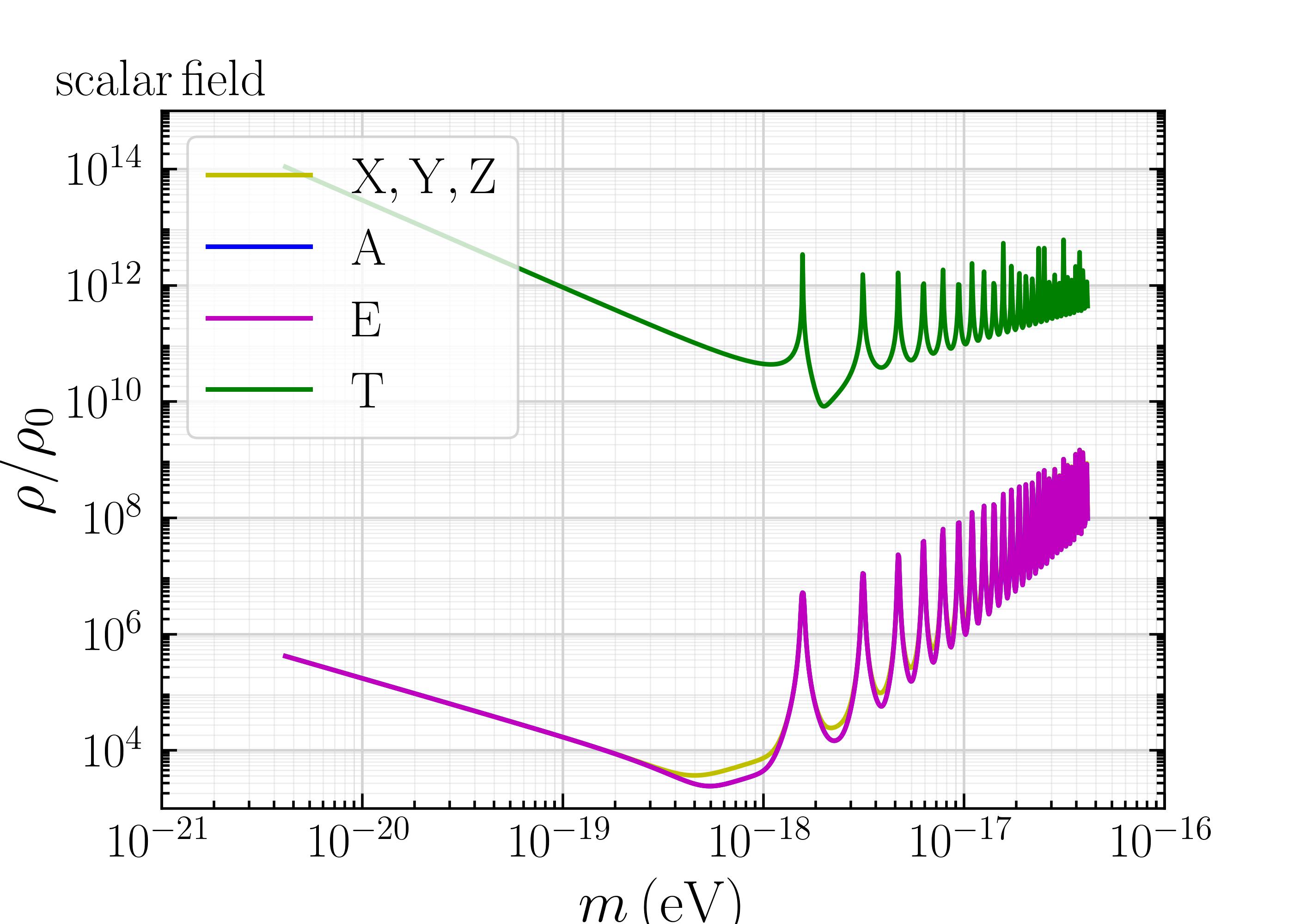
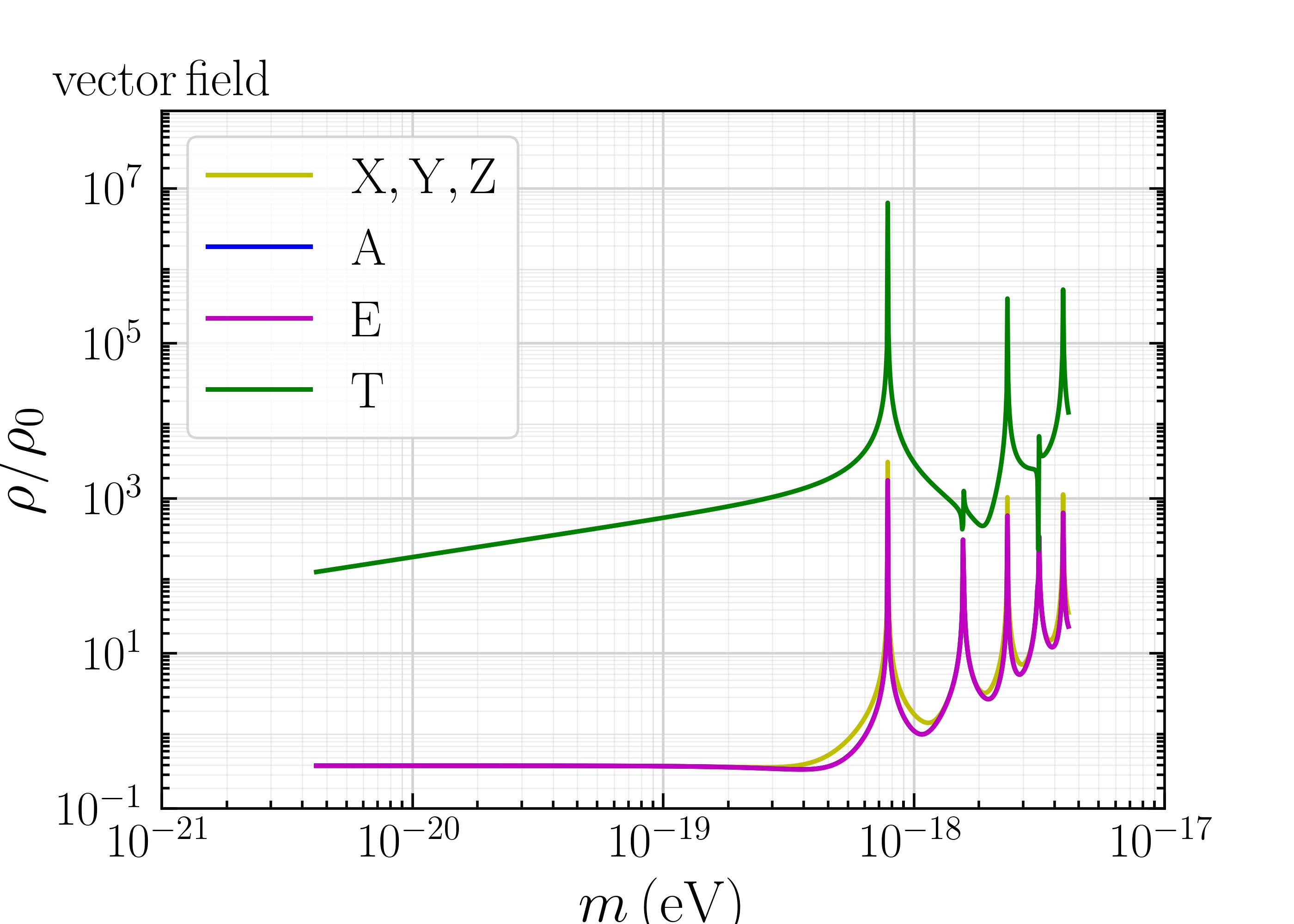
Figure S1: Projected sensitivities on $\rho$ of $\mu$Ares for scalar and vector ULDM. Michelson combinations X, Y, Z and optimal combinations A, E, T are showed. The observation time is 10 yrs.

IV Signals of other experiments

IV.1 Grace Follow-on

The run data of other laser experiments in space, such as Grace Follow-on (GRACE-FO), can also provide limits on the density of dark matter. The physical principle is very similar. The gravitational perturbation of ULDM will cause the frequency shift of photons and the displacement of the test mass, which will affect the corresponding phases. For GRACE-FO, two satellites separated by $L=200$km form a single interferometer with arm-length $2L$, and the half-round displacement noise spectrum of Grace follow-on mission is given by [98]. Then the response is given by

$$y(t)=2mL^{2}\Phi_{0}\sin 2mt-n^{i}n^{j}\epsilon_{ij}mL^{2}h_{0}\sin 2mt-vL\Psi_{0}\hat{k}\cdot\hat{n}\cos 2mt,$$ (S25)

and the Fourier amplitude in the finite observation duration $T$ is

$$\tilde{y}(\omega)\simeq(2mL^{2}\Phi_{0}-n^{i}n^{j}\epsilon_{ij}mL^{2}h_{0}-vL\Psi_{0}\hat{k}\cdot\hat{n})T.$$ (S26)

Then the power spectrum is given by

$$S(\omega)\simeq|2mL^{2}\Phi_{0}-n^{i}n^{j}\epsilon_{ij}mL^{2}h_{0}-vL\Psi_{0}\hat{k}\cdot\hat{n}|^{2}T.$$ (S27)

The first term and the third term are determined by the scalar part of the metric perturbation, and the second term is determined by the tensor part. Correspondingly the constraint on $\rho$ can be derived. For example, for vector ULDM, we have

$$\rho(f)\simeq\frac{12m^{2}}{\kappa^{2}}\sqrt{\frac{N(f)}{|-2mL^{2}+8n^{i}n^{j}\epsilon_{ij}mL^{2}+vL\hat{k}\cdot\hat{n}|^{2}}}.$$ (S28)

Considering the difference in coefficients of metric perturbations between scalar and vector fields, the coefficient 12 in the above equation should be replaced with 4 in the case of scalar field. The unit of $N(f)$ here is m/$\sqrt{\text{Hz}}$ , which is different from space-based gravitational wave detectors. The magnitude of the signal is at the same level among scalar, vector and tensor ULDM.

IV.2 Astrometric effects

For a stationary observer in the tensor perturbation described by a plane wave $h_{ij}(\xi=-v_{p}t+\vec{n}\cdot\vec{x})$ with $|\vec{n}|=1$, the apparent deviation of the angular direction of a light source from its true direction $\vec{N}$ is given by

$$\Delta N_{i}=R_{ilj}h_{lj},\quad R_{ilj}=\frac{\frac{1}{2}N_{l}N_{j}}{1+\vec{n}\cdot\vec{N}/v_{p}}(N_{i}+n_{i}/v_{p})-\frac{1}{2}N_{j}\delta_{il}.$$ (S29)

here we have extended the result for $v_{p}=1$ in [101]. For the tensor perturbations sourced by non-relativistic ULDM, we use the approximation $v_{p}=\infty$, hence

$$R_{ilj}=\frac{1}{2}N_{l}N_{j}N_{i}-\frac{1}{2}N_{j}\delta_{il}.$$ (S30)

Using the metric perturbation given by Eqs. (S13) for vector ULDM, we obtain

$$|\Delta\vec{N}(\vec{N},t)|=A|\cos(2\omega t-2\vec{k}\cdot\vec{x})|,\quad A=\frac{4}{3}\pi\frac{\rho}{m^{2}}|(N_{l}N_{j}N_{i}-N_{j}\delta_{il})\epsilon_{lj}|.$$ (S31)

An optimistic estimation for the sensitivity of a single astrometric measurement to this oscillating signal is given by $A_{\text{max}}>10\,\mu\text{as}=4.8\times 10^{-11}\,\text{rad}$ (for Gaia-like accuracy [102, 103, 104, 105]), where $A_{\text{max}}$ is the maximum value of $A$ with an optimal choice of field polarization. We can obtain $\rho/\rho_{0}>5\times 10^{10}\left(\frac{m}{10^{-20}\,\text{eV}}\right)^{2}$.

References

- Peccei and Quinn [1977] R. D. Peccei and H. R. Quinn, conservation in the presence of pseudoparticles, Phys. Rev. Lett. 38, 1440 (1977).
- Weinberg [1978] S. Weinberg, A new light boson?, Phys. Rev. Lett. 40, 223 (1978).
- Wilczek [1978] F. Wilczek, Problem of strong and invariance in the presence of instantons, Phys. Rev. Lett. 40, 279 (1978).
- Hui et al. [2017] L. Hui, J. P. Ostriker, S. Tremaine, and E. Witten, Ultralight scalars as cosmological dark matter, Phys. Rev. D 95, 043541 (2017).
- Marsh [2016] D. J. E. Marsh, Axion Cosmology, Phys. Rept. 643, 1 (2016), arXiv:1510.07633 [astro-ph.CO] .
- Agrawal et al. [2021] P. Agrawal et al., Feebly-interacting particles: FIPs 2020 workshop report, Eur. Phys. J. C 81, 1015 (2021), arXiv:2102.12143 [hep-ph] .
- Polchinski [2007] J. Polchinski, String theory, Cambridge Monographs on Mathematical Physics (Cambridge University Press, 2007).
- Wu [2022] Y.-L. Wu, Foundations of the Hyperunified Field Theory (World Scientific, 2022).
- Kim [1987] J. E. Kim, Light Pseudoscalars, Particle Physics and Cosmology, Phys. Rept. 150, 1 (1987).
- Fayet [1990] P. Fayet, Extra U(1)’s and New Forces, Nucl. Phys. B 347, 743 (1990).
- Arias et al. [2012] P. Arias, D. Cadamuro, M. Goodsell, J. Jaeckel, J. Redondo, and A. Ringwald, WISPy Cold Dark Matter, JCAP 06, 013, arXiv:1201.5902 [hep-ph] .
- Lyth and Riotto [1999] D. H. Lyth and A. Riotto, Particle physics models of inflation and the cosmological density perturbation, Phys. Rept. 314, 1 (1999), arXiv:hep-ph/9807278 .
- Graham et al. [2016] P. W. Graham, J. Mardon, and S. Rajendran, Vector Dark Matter from Inflationary Fluctuations, Phys. Rev. D 93, 103520 (2016), arXiv:1504.02102 [hep-ph] .
- Ema et al. [2019] Y. Ema, K. Nakayama, and Y. Tang, Production of purely gravitational dark matter: the case of fermion and vector boson, JHEP 07, 060, arXiv:1903.10973 [hep-ph] .
- Ahmed et al. [2020] A. Ahmed, B. Grzadkowski, and A. Socha, Gravitational production of vector dark matter, JHEP 08, 059, arXiv:2005.01766 [hep-ph] .
- Kolb and Long [2021] E. W. Kolb and A. J. Long, Completely dark photons from gravitational particle production during the inflationary era, JHEP 03, 283, arXiv:2009.03828 [astro-ph.CO] .
- Graham and Rajendran [2013] P. W. Graham and S. Rajendran, New Observables for Direct Detection of Axion Dark Matter, Phys. Rev. D 88, 035023 (2013), arXiv:1306.6088 [hep-ph] .
- Graham et al. [2015] P. W. Graham, I. G. Irastorza, S. K. Lamoreaux, A. Lindner, and K. A. van Bibber, Experimental Searches for the Axion and Axion-Like Particles, Ann. Rev. Nucl. Part. Sci. 65, 485 (2015), arXiv:1602.00039 [hep-ex] .
- Safronova et al. [2018] M. S. Safronova, D. Budker, D. DeMille, D. F. J. Kimball, A. Derevianko, and C. W. Clark, Search for New Physics with Atoms and Molecules, Rev. Mod. Phys. 90, 025008 (2018), arXiv:1710.01833 [physics.atom-ph] .
- Preskill et al. [1983] J. Preskill, M. B. Wise, and F. Wilczek, Cosmology of the Invisible Axion, Phys. Lett. B 120, 127 (1983).
- Abbott and Sikivie [1983] L. F. Abbott and P. Sikivie, A Cosmological Bound on the Invisible Axion, Phys. Lett. B 120, 133 (1983).
- Dine and Fischler [1983] M. Dine and W. Fischler, The Not So Harmless Axion, Phys. Lett. B 120, 137 (1983).
- Van Tilburg et al. [2015] K. Van Tilburg, N. Leefer, L. Bougas, and D. Budker, Search for ultralight scalar dark matter with atomic spectroscopy, Phys. Rev. Lett. 115, 011802 (2015), arXiv:1503.06886 [physics.atom-ph] .
- Chen et al. [2020] Y. Chen, J. Shu, X. Xue, Q. Yuan, and Y. Zhao, Probing Axions with Event Horizon Telescope Polarimetric Measurements, Phys. Rev. Lett. 124, 061102 (2020), arXiv:1905.02213 [hep-ph] .
- Li et al. [2024] H.-J. Li, W. Chao, and Y.-F. Zhou, Axion limits from the 10-year gamma-ray emission 1ES 1215+303, Phys. Lett. B 850, 138531 (2024), arXiv:2312.05555 [astro-ph.HE] .
- Liang et al. [2019] Y.-F. Liang, C. Zhang, Z.-Q. Xia, L. Feng, Q. Yuan, and Y.-Z. Fan, Constraints on axion-like particle properties with TeV gamma-ray observations of Galactic sources, JCAP 06, 042, arXiv:1804.07186 [hep-ph] .
- Foster et al. [2021] J. W. Foster, Y. Kahn, R. Nguyen, N. L. Rodd, and B. R. Safdi, Dark matter interferometry, Phys. Rev. D 103, 076018 (2021).
- Liu et al. [2023] T. Liu, X. Lou, and J. Ren, Pulsar Polarization Arrays, Phys. Rev. Lett. 130, 121401 (2023), arXiv:2111.10615 [astro-ph.HE] .
- Stadnik and Flambaum [2015] Y. V. Stadnik and V. V. Flambaum, Searching for dark matter and variation of fundamental constants with laser and maser interferometry, Phys. Rev. Lett. 114, 161301 (2015), arXiv:1412.7801 [hep-ph] .
- Fu et al. [2017] C. Fu et al. (PandaX), Limits on Axion Couplings from the First 80 Days of Data of the PandaX-II Experiment, Phys. Rev. Lett. 119, 181806 (2017), arXiv:1707.07921 [hep-ex] .
- Aprile et al. [2022] E. Aprile et al. (XENON), Search for New Physics in Electronic Recoil Data from XENONnT, Phys. Rev. Lett. 129, 161805 (2022), arXiv:2207.11330 [hep-ex] .
- Chao et al. [2023a] W. Chao, J.-J. Feng, and M.-J. Jin, Direct detections of the Axion-like particle Revisited, (2023a), arXiv:2311.09547 [hep-ph] .
- Budker et al. [2014] D. Budker, P. W. Graham, M. Ledbetter, S. Rajendran, and A. Sushkov, Proposal for a Cosmic Axion Spin Precession Experiment (CASPEr), Phys. Rev. X 4, 021030 (2014), arXiv:1306.6089 [hep-ph] .
- Hamaguchi et al. [2018] K. Hamaguchi, N. Nagata, K. Yanagi, and J. Zheng, Limit on the Axion Decay Constant from the Cooling Neutron Star in Cassiopeia A, Phys. Rev. D 98, 103015 (2018), arXiv:1806.07151 [hep-ph] .
- Garcon et al. [2019] A. Garcon et al., Constraints on bosonic dark matter from ultralow-field nuclear magnetic resonance, Sci. Adv. 5, eaax4539 (2019), arXiv:1902.04644 [hep-ex] .
- Centers et al. [2021] G. P. Centers et al., Stochastic fluctuations of bosonic dark matter, Nature Commun. 12, 7321 (2021), arXiv:1905.13650 [astro-ph.CO] .
- Wei et al. [2023] K. Wei et al., Dark matter search with a strongly-coupled hybrid spin system, (2023), arXiv:2306.08039 [hep-ph] .
- Ge and Murayama [2019] S.-F. Ge and H. Murayama, Apparent CPT Violation in Neutrino Oscillation from Dark Non-Standard Interactions, (2019), arXiv:1904.02518 [hep-ph] .
- Choi et al. [2020] K.-Y. Choi, E. J. Chun, and J. Kim, Neutrino Oscillations in Dark Matter, Phys. Dark Univ. 30, 100606 (2020), arXiv:1909.10478 [hep-ph] .
- Chen et al. [2023a] Y. Chen, X. Xue, and V. Cardoso, Black Holes as Neutrino Factories, (2023a), arXiv:2308.00741 [hep-ph] .
- Caputo et al. [2021] A. Caputo, A. J. Millar, C. A. J. O’Hare, and E. Vitagliano, Dark photon limits: A handbook, Phys. Rev. D 104, 095029 (2021), arXiv:2105.04565 [hep-ph] .
- Chaudhuri et al. [2015] S. Chaudhuri, P. W. Graham, K. Irwin, J. Mardon, S. Rajendran, and Y. Zhao, Radio for hidden-photon dark matter detection, Phys. Rev. D 92, 075012 (2015), arXiv:1411.7382 [hep-ph] .
- An et al. [2023] H. An, S. Ge, W.-Q. Guo, X. Huang, J. Liu, and Z. Lu, Direct Detection of Dark Photon Dark Matter Using Radio Telescopes, Phys. Rev. Lett. 130, 181001 (2023), arXiv:2207.05767 [hep-ph] .
- An et al. [2024a] H. An, X. Chen, S. Ge, J. Liu, and Y. Luo, Searching for ultralight dark matter conversion in solar corona using Low Frequency Array data, Nature Commun. 15, 915 (2024a), arXiv:2301.03622 [hep-ph] .
- An et al. [2024b] H. An, S. Ge, J. Liu, and Z. Lu, Direct Detection of Dark Photon Dark Matter with the James Webb Space Telescope, (2024b), arXiv:2402.17140 [hep-ph] .
- Chen et al. [2023b] S. Chen, H. Fukuda, T. Inada, T. Moroi, T. Nitta, and T. Sichanugrist, Detecting Hidden Photon Dark Matter Using the Direct Excitation of Transmon Qubits, Phys. Rev. Lett. 131, 211001 (2023b), arXiv:2212.03884 [hep-ph] .
- Chen et al. [2023c] S. Chen, H. Fukuda, T. Inada, T. Moroi, T. Nitta, and T. Sichanugrist, Quantum Enhancement in Dark Matter Detection with Quantum Computation, (2023c), arXiv:2311.10413 [hep-ph] .
- Chen et al. [2024] Y. Chen, C. Li, Y. Liu, Y. Liu, J. Shu, and Y. Zeng, SRF Cavity as Galactic Dark Photon Telescope, (2024), arXiv:2402.03432 [hep-ph] .
- Tang et al. [2023] Z. Tang et al., SRF Cavity Searches for Dark Photon Dark Matter: First Scan Results, (2023), arXiv:2305.09711 [hep-ex] .
- Chao et al. [2023b] W. Chao, J.-j. Feng, H.-k. Guo, and T. Li, Oscillations of Ultralight Dark Photon into Gravitational Waves, (2023b), arXiv:2312.04017 [hep-ph] .
- Pierce et al. [2018] A. Pierce, K. Riles, and Y. Zhao, Searching for dark photon dark matter with gravitational-wave detectors, Phys. Rev. Lett. 121, 061102 (2018).
- Morisaki and Suyama [2019] S. Morisaki and T. Suyama, Detectability of ultralight scalar field dark matter with gravitational-wave detectors, Phys. Rev. D 100, 123512 (2019).
- Guo et al. [2019] H.-K. Guo, Y. Ma, J. Shu, X. Xue, Q. Yuan, and Y. Zhao, Detecting dark photon dark matter with Gaia-like astrometry observations, JCAP 05, 015, arXiv:1902.05962 [hep-ph] .
- Fukusumi et al. [2023] K. Fukusumi, S. Morisaki, and T. Suyama, Upper limit on scalar field dark matter from ligo-virgo third observation run (2023), arXiv:2303.13088 [hep-ph] .
- Yu et al. [2023] J.-C. Yu, Y.-H. Yao, Y. Tang, and Y.-L. Wu, Sensitivity of space-based gravitational-wave interferometers to ultralight bosonic fields and dark matter, Phys. Rev. D 108, 083007 (2023).
- Khmelnitsky and Rubakov [2014] A. Khmelnitsky and V. Rubakov, Pulsar timing signal from ultralight scalar dark matter, JCAP 02, 019, arXiv:1309.5888 [astro-ph.CO] .
- Porayko and Postnov [2014] N. K. Porayko and K. A. Postnov, Constraints on ultralight scalar dark matter from pulsar timing, Phys. Rev. D 90, 062008 (2014), arXiv:1408.4670 [astro-ph.CO] .
- Aoki and Soda [2016] A. Aoki and J. Soda, Detecting ultralight axion dark matter wind with laser interferometers, Int. J. Mod. Phys. D 26, 1750063 (2016), arXiv:1608.05933 [astro-ph.CO] .
- Nomura et al. [2020] K. Nomura, A. Ito, and J. Soda, Pulsar timing residual induced by ultralight vector dark matter, Eur. Phys. J. C 80, 419 (2020), arXiv:1912.10210 [gr-qc] .
- Sun et al. [2022] S. Sun, X.-Y. Yang, and Y.-L. Zhang, Pulsar timing residual induced by wideband ultralight dark matter with spin 0,1,2, Phys. Rev. D 106, 066006 (2022), arXiv:2112.15593 [astro-ph.CO] .
- Wu et al. [2023] Y.-M. Wu, Z.-C. Chen, and Q.-G. Huang, Pulsar timing residual induced by ultralight tensor dark matter, JCAP 09, 021, arXiv:2305.08091 [hep-ph] .
- Guo et al. [2023] R.-Z. Guo, Y. Jiang, and Q.-G. Huang, Probing Ultralight Tensor Dark Matter with the Stochastic Gravitational-Wave Background from Advanced LIGO and Virgo’s First Three Observing Runs, (2023), arXiv:2312.16435 [astro-ph.CO] .
- Cai et al. [2024] R.-G. Cai, J.-R. Zhang, and Y.-L. Zhang, Angular correlation and deformed Hellings-Downs curve by spin-2 ultralight dark matter, (2024), arXiv:2402.03984 [gr-qc] .
- Xue et al. [2022] X. Xue et al. (PPTA), High-precision search for dark photon dark matter with the Parkes Pulsar Timing Array, Phys. Rev. Res. 4, L012022 (2022), arXiv:2112.07687 [hep-ph] .
- Kim [2023] H. Kim, Gravitational interaction of ultralight dark matter with interferometers, JCAP 12, 018, arXiv:2306.13348 [hep-ph] .
- Kim and Mitridate [2024] H. Kim and A. Mitridate, Stochastic ultralight dark matter fluctuations in pulsar timing arrays, Phys. Rev. D 109, 055017 (2024), arXiv:2312.12225 [hep-ph] .
- Pitjev and Pitjeva [2013] N. P. Pitjev and E. V. Pitjeva, Constraints on dark matter in the solar system, Astronomy Letters 39, 141–149 (2013).
- Blas et al. [2017] D. Blas, D. L. Nacir, and S. Sibiryakov, Ultralight Dark Matter Resonates with Binary Pulsars, Phys. Rev. Lett. 118, 261102 (2017), arXiv:1612.06789 [hep-ph] .
- Blas et al. [2020] D. Blas, D. López Nacir, and S. Sibiryakov, Secular effects of ultralight dark matter on binary pulsars, Phys. Rev. D 101, 063016 (2020), arXiv:1910.08544 [gr-qc] .
- Yuan et al. [2022] G.-W. Yuan, Z.-Q. Shen, Y.-L. S. Tsai, Q. Yuan, and Y.-Z. Fan, Constraining ultralight bosonic dark matter with Keck observations of S2’s orbit and kinematics, Phys. Rev. D 106, 103024 (2022), arXiv:2205.04970 [astro-ph.HE] .
- Armengaud et al. [2017] E. Armengaud, N. Palanque-Delabrouille, C. Yèche, D. J. E. Marsh, and J. Baur, Constraining the mass of light bosonic dark matter using SDSS Lyman- forest, Mon. Not. Roy. Astron. Soc. 471, 4606 (2017), arXiv:1703.09126 [astro-ph.CO] .
- Iršič et al. [2017] V. Iršič, M. Viel, M. G. Haehnelt, J. S. Bolton, and G. D. Becker, First constraints on fuzzy dark matter from lyman- forest data and hydrodynamical simulations, Phys. Rev. Lett. 119, 031302 (2017).
- Kobayashi et al. [2017] T. Kobayashi, R. Murgia, A. De Simone, V. Iršič, and M. Viel, Lyman- constraints on ultralight scalar dark matter: Implications for the early and late universe, Phys. Rev. D 96, 123514 (2017), arXiv:1708.00015 [astro-ph.CO] .
- Schneider [2018] A. Schneider, Constraining noncold dark matter models with the global 21-cm signal, Phys. Rev. D 98, 063021 (2018), arXiv:1805.00021 [astro-ph.CO] .
- Lidz and Hui [2018] A. Lidz and L. Hui, Implications of a prereionization 21-cm absorption signal for fuzzy dark matter, Phys. Rev. D 98, 023011 (2018), arXiv:1805.01253 [astro-ph.CO] .
- Arvanitaki and Dubovsky [2011] A. Arvanitaki and S. Dubovsky, Exploring the String Axiverse with Precision Black Hole Physics, Phys. Rev. D 83, 044026 (2011), arXiv:1004.3558 [hep-th] .
- Brito et al. [2015] R. Brito, V. Cardoso, and P. Pani, Superradiance: New Frontiers in Black Hole Physics, Lect. Notes Phys. 906, pp.1 (2015), arXiv:1501.06570 [gr-qc] .
- Arvanitaki et al. [2017] A. Arvanitaki, M. Baryakhtar, S. Dimopoulos, S. Dubovsky, and R. Lasenby, Black Hole Mergers and the QCD Axion at Advanced LIGO, Phys. Rev. D 95, 043001 (2017), arXiv:1604.03958 [hep-ph] .
- Brito et al. [2017] R. Brito, S. Ghosh, E. Barausse, E. Berti, V. Cardoso, I. Dvorkin, A. Klein, and P. Pani, Gravitational wave searches for ultralight bosons with LIGO and LISA, Phys. Rev. D 96, 064050 (2017), arXiv:1706.06311 [gr-qc] .
- Davoudiasl and Denton [2019] H. Davoudiasl and P. B. Denton, Ultralight Boson Dark Matter and Event Horizon Telescope Observations of M87*, Phys. Rev. Lett. 123, 021102 (2019), arXiv:1904.09242 [astro-ph.CO] .
- Cao and Tang [2023] Y. Cao and Y. Tang, Signatures of ultralight bosons in compact binary inspiral and outspiral, Phys. Rev. D 108, 123017 (2023), arXiv:2307.05181 [gr-qc] .
- Bar et al. [2018] N. Bar, D. Blas, K. Blum, and S. Sibiryakov, Galactic rotation curves versus ultralight dark matter: Implications of the soliton-host halo relation, Phys. Rev. D 98, 083027 (2018), arXiv:1805.00122 [astro-ph.CO] .
- Marsh and Niemeyer [2019] D. J. E. Marsh and J. C. Niemeyer, Strong Constraints on Fuzzy Dark Matter from Ultrafaint Dwarf Galaxy Eridanus II, Phys. Rev. Lett. 123, 051103 (2019), arXiv:1810.08543 [astro-ph.CO] .
- Bar et al. [2019] N. Bar, K. Blum, J. Eby, and R. Sato, Ultralight dark matter in disk galaxies, Phys. Rev. D 99, 103020 (2019), arXiv:1903.03402 [astro-ph.CO] .
- Safarzadeh and Spergel [2019] M. Safarzadeh and D. N. Spergel, Ultra-light Dark Matter is Incompatible with the Milky Way’s Dwarf Satellites 10.3847/1538-4357/ab7db2 (2019), arXiv:1906.11848 [astro-ph.CO] .
- Note [1] We find tensor ULDM has similar behaviors as scalar ULDM.
- Amaro-Seoane et al. [2017] P. Amaro-Seoane et al., Laser interferometer space antenna (2017), arXiv:1702.00786 [astro-ph.IM] .
- Hu and Wu [2017] W.-R. Hu and Y.-L. Wu, The Taiji Program in Space for gravitational wave physics and the nature of gravity, National Science Review 4, 685 (2017), https://academic.oup.com/nsr/article-pdf/4/5/685/31566708/nwx116.pdf .
- Luo et al. [2016] J. Luo et al., Tianqin: a space-borne gravitational wave detector, Classical and Quantum Gravity 33, 035010 (2016).
- Crowder and Cornish [2005] J. Crowder and N. J. Cornish, Beyond lisa: Exploring future gravitational wave missions, Phys. Rev. D 72, 083005 (2005).
- Kawamura et al. [2006] S. Kawamura et al., The japanese space gravitational wave antenna—decigo, Classical and Quantum Gravity 23, S125 (2006).
- Sesana et al. [2021] A. Sesana et al., Unveiling the gravitational universe at -hz frequencies, Experimental Astronomy 51, 1333–1383 (2021).
- Martens et al. [2023] W. Martens, M. Khan, and J.-B. Bayle, Lisamax: Improving the low-frequency gravitational-wave sensitivity by two orders of magnitude (2023), arXiv:2304.08287 [gr-qc] .
- NI [2013] W.-T. NI, Astrod-gw: Overview and progress, International Journal of Modern Physics D 22, 1341004 (2013).
- Tinto and Dhurandhar [2021] M. Tinto and S. V. Dhurandhar, Time-delay interferometry, Living Rev. Rel. 24, 1 (2021).
- Babak et al. [2021] S. Babak, A. Petiteau, and M. Hewitson, LISA Sensitivity and SNR Calculations, (2021), arXiv:2108.01167 [astro-ph.IM] .
- Note [2] Here we focus on the deterministic monochromatic signal, other than the stochastic continuous component at lower frequencies [65], which has no boost factor in PSD if there is no an additional detector for correlation analysis.
- Abich et al. [2019] K. Abich, , et al., In-orbit performance of the grace follow-on laser ranging interferometer, Phys. Rev. Lett. 123, 031101 (2019).
- Costa and Natario [2014] L. F. O. Costa and J. Natario, Gravito-electromagnetic analogies, Gen. Rel. Grav. 46, 1792 (2014), arXiv:1207.0465 [gr-qc] .
- Prince et al. [2002] T. A. Prince, M. Tinto, S. L. Larson, and J. W. Armstrong, The LISA optimal sensitivity, Phys. Rev. D 66, 122002 (2002), arXiv:gr-qc/0209039 .
- Book and Flanagan [2011] L. G. Book and E. E. Flanagan, Astrometric Effects of a Stochastic Gravitational Wave Background, Phys. Rev. D 83, 024024 (2011), arXiv:1009.4192 [astro-ph.CO] .
- Collaboration [2022] G. Collaboration, Gaia data release 3: Summary of the content and survey properties, (2022), arXiv:2208.00211 [astro-ph.GA] .
- Moore et al. [2017] C. J. Moore, D. P. Mihaylov, A. Lasenby, and G. Gilmore, Astrometric Search Method for Individually Resolvable Gravitational Wave Sources with Gaia, Phys. Rev. Lett. 119, 261102 (2017), arXiv:1707.06239 [astro-ph.IM] .
- Jaraba et al. [2023] S. Jaraba, J. García-Bellido, S. Kuroyanagi, S. Ferraiuolo, and M. Braglia, Stochastic gravitational wave background constraints from Gaia DR3 astrometry, Mon. Not. Roy. Astron. Soc. 524, 3609 (2023), arXiv:2304.06350 [astro-ph.CO] .
- Mentasti and Contaldi [2023] G. Mentasti and C. R. Contaldi, Observing gravitational waves with solar system astrometry, (2023), arXiv:2311.03474 [gr-qc] .