Bipartite Fluctuations of Critical Fermi Surfaces

Abstract

We investigate the scaling behaviors of bipartite fluctuations $\mathcal{F}$ of conserved quantities across a class of interaction-driven quantum phase transitions out of Landau fermi liquids, where other phases involve fermi-surface states of fractionalized degrees of freedom. Examples of such phases include (compressible) composite fermi liquids for spinless electrons and (incompressible) spin-liquid Mott insulators for spin-$1/2$ electrons. The two sides of the critical points are typically distinguished by distinct leading-order scalings of bipartite charge fluctuations, $\mathcal{F}\sim L\log(L)$ in Landau fermi liquids, and $\mathcal{F}\sim L$ in the other phases, where $L$ is the linear size of the subsystem under bipartition. In the case of composite fermi liquids (with continuous translational and rotational invariance), we also identify a universal constant term $-\mathtt{F}(\theta)\sigma_{xy}/\pi$ arising when the subsystem geometry incorporates a sharp corner. Here, $\mathtt{F}(\theta)$ represents a function of the corner angle, and $\sigma_{xy}$ denotes the Hall conductivity. At the critical point of each example, we find that the leading-order scaling $\mathcal{F}\sim L$ is accompanied by a subleading universal corner contribution $-\mathtt{F}(\theta)C_{\rho}\log(L)$ with the same angle dependence $\mathtt{F}(\theta)$. The universal coefficient $C_{\rho}$ is linked to the predicted universal longitudinal (and Hall) resistivity jump $\Delta\rho_{xx}$ (and $\Delta\rho_{xy}$) at the critical point.

I Introduction

Bipartite fluctuations of local observables offer crucial insight into entanglement properties, symmetries, and correlations in many-body quantum systems. Although entanglement has become a fundamental organizing principle for the study of quantum matter [1, 2], experimental measurement of many-body entanglement remains a challenge. Significant progress (see, e.g., Ref. [3, 4, 5, 6, 7, 8, 9, 10, 11, 12]) has been made toward establishing a direct relationship between entanglement entropy and the fluctuations of globally conserved quantities, such as particle number and magnetization. This relationship has been demonstrated to be feasible in special cases, such as one-dimensional Luttinger liquids [6, 8] and free fermions in higher dimensions [9, 8, 4]. However, the connection between the two in strongly correlated systems beyond these examples is still poorly understood. The two quantities are observed to differ from each other in continuous symmetry-breaking phases, where the entanglement entropy still follows a boundary-law scaling while the bipartite fluctuations exhibit a multiplicative logarithmic enhancement to the boundary law. Building on this observation, Ref. [13] proposed the use of the distinct scalings of bipartite fluctuations to detect conventional Landau phase transitions.

Despite decades of study, understanding unconventional quantum phases and phase transitions that are beyond Landau’s symmetry-breaking paradigm remains a central problem in condensed matter physics. In recent years, conceptual breakthroughs [14, 15] have been achieved by employing extended operators to define generalized symmetries and to characterize phases and phase transitions (see Ref. [16, 17] and references therein). For instance, abelian topological orders can be understood in terms of the condensation of 1-dimensional objects, leading to the spontaneous breaking of discrete $1$-form symmetries. Similarly, the Coulomb phase of electrodynamics can be interpreted as a spontaneous symmetry-breaking phase of $\textrm{U}(1)$ $1$-form symmetry, where gapless photons serve as Goldstone modes. This helps establish a generalized Landau symmetry paradigm. In this case, the criterion for determining whether the phase is symmetric or not is given by the scaling of disorder operators (or Wilson loops under duality). In this context, the concept of bipartite fluctuations is again closely related, which can be identified as the $\textrm{U}(1)$ disorder operator under the small-angle limit [18, 19].

While extended operators play an important role in the conceptual understanding of phases of matter, recent studies have also shed light on intriguing quantitative aspects of disorder operators (and related bipartite fluctuations), particularly their scaling behaviors at conformally invariant quantum critical points [18, 19, 20, 21, 22, 23, 24, 25]. For instance, when considering the configuration of the subsystem as depicted in FIG. 1, bipartite fluctuations exhibit a universal corner contribution with logarithmic scaling. This contribution has a universal angle dependence and is directly proportional to the current central charge $C_{J}$ of the conformal field theory (CFT) [18, 19, 20]. Given the sometimes uncertain fate of proposed lattice realizations for exotic quantum critical points, numerical simulations, such as quantum Monte Carlo simulations, can assist in identifying whether these lattice models correspond to unitary CFTs by examining the sign of the universal corner contribution to disorder operators [21, 22, 23, 24, 25].

Understanding quantum phase transitions in metals is significantly more challenging due to the abundance of low-energy excitations near the electronic fermi surface. Even for conventional phase transitions associated with some form of broken symmetry in metals, the standard Hertz-Millis-Moriya framework [26, 27, 28] encounters serious difficulties in two spatial dimensions. Despite numerous attempts made in recent years [29, 30, 31, 32, 33, 34, 35, 36, 37, 38, 39, 40, 41, 42, 43, 44, 45, 46], many aspects of the low-energy physics remain difficult to describe theoretically. A scenario that is both technically and conceptually more challenging is a continuous transition from an ordinary metal to an exotic gapless phase with abundant fractionalized excitations forming a fermi surface. One such example is the proposed continuous Mott transition at half-filling [47, 48, 49, 50] from a Landau fermi liquid (FL) to a gapless Mott insulator (MI) with a spinon fermi surface. This is potentially realized by the recent experimental observation [51] of a continuous bandwidth-tuned transition from a metal to a paramagnetic Mott insulator in the transition metal dichalcogenide (TMD) Moiré heterobilayer $\textrm{MoTe}_{2}/\textrm{WSe}_{2}$. However, the observed critical resistivity is anomalously large [51], exceeding the predictions of the original theory, at least in the clean limit . To address this discrepancy, Ref. [53] has proposed a modified theory that explains the large critical resistivity by charge fractionalization.

Another notable example that has appeared in literature is the continuous transition from a Landau fermi liquid to a composite fermi liquid (CFL) describing the half-filled Landau level. The theoretical possibility was originally proposed by Ref. [54] and later refined by Ref. [55] targeting TMD Moiré materials . All these examples share a common theoretical framework, which we will review in Sec. III, where electrons are fractionalized into fermionic and bosonic partons. The fermion sector forms a stable fermi-surface state, while the boson sector contains a single relevant operator that drives the transition. Crucial insight into the possible transitions comes from the filling constraints of the bosons under translation symmetry and the Lieb-Schultz-Mattis theorem [53, 55]. Without better terminology, we refer to this type of quantum critical points as “critical fermi surfaces,” following Refs. [49, 50].

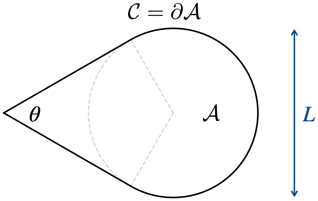
Figure 1: The real-space subsystem $\mathcal{A}$ with only one corner angle $0<\theta<\pi$. The linear size of $\mathcal{A}$ is denoted by $L$.

One of the main contributions of this paper is to point out the universal features of critical fermi surfaces from the perspective of bipartite charge fluctuations $\mathcal{F}$. Although the transitions go beyond any symmetry principles, including the generalized ones [16, 17], the two phases can be distinguished by the distinct scalings $\mathcal{F}\sim L$ and $\mathcal{F}\sim L\log(L)$, just like conventional symmetry-breaking transitions [13], where $L$ is the linear size of the subsystem under bipartition. Moreover, at the critical point, we find a universal corner contribution with logarithmic scaling, reminiscent of the behavior seen in CFTs, despite the absence of conformal symmetry in such systems. The universal coefficient (denoted by $C_{\rho}$) of the logarithmic term can be directly linked to transport observables, such as the predicted longitudinal (and Hall) resistivity jump [50, 53, 55] at the critical point.

In contrast to conformally invariant quantum critical points, many powerful theoretical tools, such as the conformal bootstrap [57], are no longer applicable to strongly correlated metals. However, it is theoretically feasible in Monte Carlo simulations [21, 22, 23, 24, 25] to extract the sub-leading universal corner term of $\mathcal{F}$ using the method proposed in Ref. [58]. We anticipate that our findings, which establish a connection between the universal data $C_{\rho}$ of the critical points and charge fluctuations which are numerically and experimentally accessible, could aid future studies in identifying the existence and lattice realizations of these exotic quantum critical points in metals.

II Preliminaries and Summary of Results

In this section, we begin with a brief introduction to some preliminaries regarding bipartite fluctuations in various phases of matter. Subsequently, we summarize our main findings regarding a class of quantum phase transitions out of Landau fermi liquids. This also serves as an outline for the remainder of the paper.

II.1 Preliminaries

For systems with a $\textrm{U}(1)$ global symmetry, the bipartite fluctuations can be defined as

$$\mathcal{F}_{\mathcal{A}}=\left\langle\left(\int_{\mathcal{A}}J^{\tau}\right)-\left\langle\int_{\mathcal{A}}J^{\tau}\right\rangle\right\rangle^{2}.$$ (1)

Here, $J^{\tau}$ represents the zeroth component of the conserved Noether current $J^{\mu}$ satisfying $\partial_{\mu}J^{\mu}=0$, and $\mathcal{A}$ is a spatial subregion within the total system. The expectation value is taken with respect to the ground state at zero temperature. By definition, the large-scale scaling behavior of $\mathcal{F}_{\mathcal{A}}$ is ultimately governed by the long-wavelength behavior of the equal-time density-density correlation $\Pi^{\tau\tau}=\langle J^{\tau}J^{\tau}\rangle$. In Sec. IV, we undertake the task of evaluating $\mathcal{F}_{\mathcal{A}}$ assuming a generic power-law instantaneous charge correlation in two dimensions. The results are summarized in TABLE. 1.

The simplest compressible state is given by the free fermi gas. Utilizing the free-fermion propagator, one can easily obtain $\Pi^{\tau\tau}(\tau\rightarrow 0,\bm{x})$ in real space or the static structure factor $\Pi^{\tau\tau}(\tau\rightarrow 0,\bm{k})$ in momentum space

$$\Pi^{\tau\tau}(\tau\rightarrow 0,\bm{x}) =\frac{k_{F}}{4\pi^{3}}\frac{1}{|\bm{x}|^{3}},$$

$$\Pi^{\tau\tau}(\tau\rightarrow 0,\bm{k}) =-\frac{k_{F}|\bm{k}|}{2\pi^{2}},$$ (2)

where $k_{F}$ denotes the fermi momentum. According to TABLE. 1, we observe the scaling $\mathcal{F}\sim L\log(L)$. This is a well-known result based on the relationship between $\mathcal{F}$ and entanglement entropy [59, 60, 61, 62, 9, 8, 4]. In Appendix A, we reproduce Eq. 2 based the $\textrm{LU}(1)$ anomaly of fermi surface states [44], which holds even in the presence of strong forward scattering preserving the $\textrm{LU}(1)$ symmetry. The bonus is a geometric interpretation  of the static structure factor through the area difference when shifting the fermi surface, as depicted in Fig. 3.

Another simple compressible state is provided by the superfluid phase. Let us denote the $\textrm{U}(1)$ order parameter by $\phi$. The gapless Goldstone mode $\theta$ corresponds to the angle fluctuation of $\phi=\rho_{s}e^{\mathtt{i}\theta}$, where $\rho_{s}$ represents the stiffness. Since the power counting of the action $\int\textrm{d}^{3}x(\partial\theta)^{2}$ yields a scaling dimension of $\Delta[\partial\theta]=3/2$ for the $\textrm{U}(1)$ charge density, the corresponding equal-time correlation scales as $|\bm{x}|^{-3}$. Once again, one finds the scaling of bipartite fluctuations $\mathcal{F}\sim L\log(L)$.

An important class of incompressible states is given by unitary CFTs. The two-point function of the conserved spin-$1$ current has a rigid structure [57]

$$\left\langle J^{\mu}(x)J^{\nu}(0)\right\rangle=\frac{C_{J}}{|x|^{4}}\left(\delta_{\mu\nu}-\frac{2x^{\mu}x^{\nu}}{|x|^{2}}\right),$$ (3)

where the scaling dimension of $J^{\mu}$ is protected. The overall coefficient $C_{J}>0$, known as the current central charge, is a universal data of the CFT and is related to the longitudinal conductivity via $\sigma_{xx}=\frac{\pi^{2}}{2}C_{J}$. Considering the subsystem with a single corner, as shown in FIG. 1, one can verify the scaling behavior [18, 20, 19]

$$\mathcal{F}=\#L-C_{J}\mathtt{F}(\theta)\log(L)+\ldots.$$ (4)

where $\#$ is a non-universal number depending on the UV cut-off, and the universal angle dependence

$$\mathtt{F}(\theta)=\frac{1}{2}(1+(\pi-\theta)\cot\theta).$$ (5)

applies to any $(2+1)$-dimensional CFTs.

Insulators with a charge gap represent another standard type of incompressible states. Due to the exponential decay of the equal-time density-density correlation, the leading-order scaling obeys the boundary law, which is the same as CFTs. An intriguing observation from Ref. [20] is that quantum Hall insulators exhibit a universal corner contribution $-(\nu/2\pi^{2})\mathtt{F}(\theta)$, considering the shape of $\mathcal{A}$ shown in FIG. 1. The angle dependence is once again given by Eq. 5, and $\nu$ denotes the filling factor. The corner term for $\nu\in\mathbb{Z}$ can be derived analytically, while the fractional quantum Hall insulator at $\nu=1/3$ has been verified using Monte Carlo simulations based on the Laughlin wave function [20].

	Leading-order term	Universal term
$2<\alpha<3$	$L^{4-\alpha}$	$L^{4-\alpha}$
$\alpha=3$	$L\log(L)$	$L\log(L)$
$3<\alpha<4$	$L/\epsilon^{\alpha-3}$	$L^{4-\alpha}$
$\alpha=4$	$L/\epsilon$	$\log(L)$
$\alpha>4$	$L/\epsilon^{\alpha-3}$	$0$

Table 1: The scaling behaviors of the bipartite fluctuations $\mathcal{F}_{\mathcal{A}}$ based on the equal-time density-density correlation $\Pi^{\tau\tau}(\tau\rightarrow 0,\bm{x})\sim|\bm{x}|^{-\alpha}$ in two dimensions. Here, $L$ represents the linear size of $\mathcal{A}$, and $\epsilon$ is a gauge-invariant UV cut-off introduced in Eq. 21. The “universal term” here is defined by the independence of the cut-off $\epsilon$. There are some notable features. The leading-order term exhibits boundary-law scaling when $\alpha>3$. The universal subleading logarithmic term exists only when $\alpha=4$ and the geometry of $\mathcal{A}$ contains any sharp corners. For $\alpha>4$, the universal subleading term approaches zero in the large-$L$ limit.

II.2 Summary of Results

Before delving into examples of critical fermi surfaces in Sec. V and Sec. VI, we provide some useful general discussions in Sec. III and Sec. IV. In Sec. V, we establish a unified theoretical framework by introducing vortex excitations in fermi liquids. Different exotic gapless phases can be then realized by putting vortices in different states. Within the vortex theory, the $\textrm{U}(1)$ disorder operator is represented by a (spatial) Wilson loop of an emergent gauge field. In Sec. IV, we offer technical details on how to regularize and calculate the Wilson loop. To better understand contributions stemming from exotic gapless modes, such as those in composite fermi liquids, we derive the general results in TABLE. 1 allowing the gauge field to have a generic tunable scaling dimension.

Below, we summarize the key results in Sec. V and Sec. VI, where we consider examples of clean electron systems at half-filling, assuming disorder effects are weak.

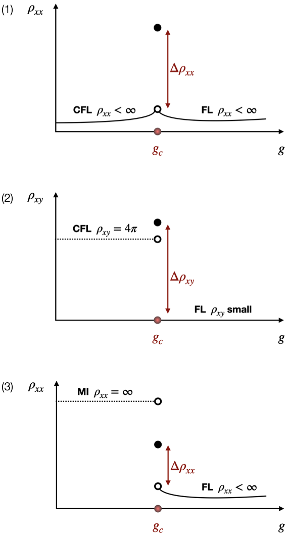
Figure 2: (1) and (2) depict the predicted universal longitudinal resistivity jump $\Delta\rho_{xx}$ and Hall resistivity jump $\Delta\rho_{xy}$ at the transition between a fermi liquid (FL) and a composite fermi liquid (CFL) [55]; (3) illustrates the predicted universal longitudinal resistivity jump $\Delta\rho_{xx}$ at the transition between a fermi liquid (FL) and a Mott insulator (MI) [50, 53]. In all of these phase transitions, the tuning parameter $g$ is related to the electron bandwidth, and the critical resistivity jumps are linked to the universal corner contribution of bipartite charge fluctuations, as described by Eq. 8.

1. Composite fermi liquids, despite being compressible, obey the boundary-law scaling $\mathcal{F}\sim L$ of bipartite charge fluctuations, contrasting with the $\mathcal{F}\sim L\log(L)$ scaling observed in other compressible states like fermi liquids and superfluid. This is because the instantaneous charge correlation from the gapless modes decays as $|\bm{x}|^{-5}$ (up to logarithmic corrections). Additionally, the gapped modes contribute a universal corner contribution, reminiscent of the behaviors seen in quantum Hall insulators [20]. Considering the geometry depicted in FIG. 1, the final result for $\nu=1/2$ reads

   $$\mathcal{F}=\#L-\frac{\sigma_{xy}}{\pi}\mathtt{F}(\theta)+\ldots.$$ (6)

   Here, $\#$ denotes a non-universal constant. The universal coefficient is determined by the DC Hall conductivity $\sigma_{xy}=\frac{1}{4\pi}$ for the composite fermi liquid with continuous translational and rotational invariance. The angle dependence remains governed by the “super-universal” formula Eq. 5.

2. At the critical point of the transition from Landau fermi liquids to composite fermi liquids, we find that the long-wavelength behavior of the static structure factor follows $|\bm{k}|^{2}\log(1/|\bm{k}|)$. Despite the absence of conformal symmetry in the system, this behavior leads to the identical scaling of bipartite fluctuations as in CFTs (c.f. Eq. 4)

   $$\mathcal{F}=\#L-C_{\rho}\mathtt{F}(\theta)\log(L)+\ldots.$$ (7)

   The coefficient $C_{\rho}$  of the corner contribution should be understood as universal data associated with the critical fermi surface. An important phenomenology of this type of transition is the universal jumps of longitudinal resistivity $\Delta\rho_{xx}(\omega/T)$ and Hall resistivity $\Delta\rho_{xy}(\omega/T)$ at the critical point [55], as depicted schematically in FIG. 2. Under the limit $\omega/T\rightarrow\infty$, these jumps are related to the universal coefficient $C_{\rho}$ through the equation

   $$C_{\rho}=\frac{2}{\pi^{2}}\frac{\Delta\rho_{xx}}{(\Delta\rho_{xx})^{2}+(\Delta\rho_{xy})^{2}}.$$ (8)

3. The continuous Mott transition [50] can be detected by the distinct scaling behaviors of bipartite charge fluctuations, $\mathcal{F}^{c}\sim L\log(L)$ in the metal phase, and $\mathcal{F}^{c}\sim L$ in the insulator phase. Once again, at the transition, the conformally non-invariant quantum critical point exhibits CFT-like behavior in the static structure factor at long wavelengths. The scaling of bipartite charge fluctuations $\mathcal{F}^{c}$ again follows Eq. 7 with the coefficient $C_{\rho}$ given by the current central charge $C_{J}^{(\textrm{XY})}$ of the 3D XY universality class. The behavior of the critical transport is simpler due to the vanishing Hall response. The relation Eq. 8 to critical resistivity jump still holds, where $\Delta\rho_{xy}=0$. Additionally, the system possesses a spin $\textrm{U}(1)$ symmetry, allowing the definition of bipartite spin fluctuations $\mathcal{F}^{s}$ accordingly. The fermi-surface states of spin fluctuations in both phases are manifested as $\mathcal{F}^{s}\sim L\log(L)$. Richer physics can be revealed by generalizing the vortex theory in Sec. III to involve both charge and spin vortices. Further insights into the multicritical behaviors will be elaborated upon in Sec. VI.2.

4. In the modified proposal [53] of the continuous Mott transition involving charge fractionalization, bipartite charge fluctuations $\mathcal{F}^{c}$ still exhibit distinct behaviors in two phases, characterized by scalings of $\mathcal{F}^{c}\sim L\log(L)$ and $\mathcal{F}^{c}\sim L$. A crucial distinction from the original theory [50] is observed in $\mathcal{F}^{c}$ at the critical point, where it follows Eq. 7 with a suppressed universal coefficient $C_{\rho}=2C_{J}^{(\textrm{XY})}/N^{2}$, where $C_{J}^{(\textrm{XY})}$ still denotes the current central charge of the 3D XY fixed point. Here, $N$, an even integer, corresponds to the fractional electric charge $e/N$ carried by each charge carrier. Notably, in the time-reversal invariant scenario described by Eq. 8 with $\Delta\rho_{xy}=0$, the critical resistivity jump $\Delta\rho_{xx}$ experiences an enhancement by a factor of $N^{2}/2$, consistent with the experimentally observed large critical resistivity [51]. Another deviation from the original theory is observed in the behavior of bipartite spin fluctuations $\mathcal{F}^{s}$, which exhibit boundary-law scaling $\mathcal{F}^{s}\sim L$ in the Mott insulator phase.

	(1) FL-CFL transition	(2) Mott transition	(3) Mott transition	$\ldots$
electron $c$	spinless $c(\bm{x})=b(\bm{x})f(\bm{x})$	spinful $c_{\sigma}(\bm{x})=b(\bm{x})f_{\sigma}(\bm{x})$	spinful $c_{\sigma}(\bm{x})=b_{\sigma}(\bm{x})f_{\sigma}(\bm{x})$	$\ldots$
fermion $f$	fermi surface	fermi surface	fermi surface	fermi surface
boson $b$	superfluid to Laughlin at $\nu=1/2$	superfluid to trivial gapped	superfluid to $Z_{N}$ topological order	superfluid to …
vortex $v$	trivial gapped to IQH at $\nu=-2$	trivial gapped to Higgs	trivial gapped to Higgs $\textrm{U}(1)\rightarrow Z_{N}$	trivial to …

Table 2: The parton constructions $c\sim bf$ for the quantum phase transitions out of spinless and spin-$1/2$ Landau fermi liquids at half-filling, where $\sigma=\uparrow,\downarrow$ represents the spin quantum number. The dual vortex $v$ is introduced in Eq. 11.

III Vortex Theory Framework

In this section, we present a general theoretical framework for describing a class of quantum phase transitions out of Landau fermi liquids, which will be utilized repeatedly in this paper.

One route to quantum phase transitions is to incorporate vortex excitations in the Landau fermi liquid phase of electrons. If the vortex sector is not trivially gapped, the system is driven into a different phase. To formulate the idea, it is sometimes convenient to start with a parton decomposition of the spin-$1/2$ or spinless electron operator $c({\bm{x}})$, given by

$$c({\bm{x}})=b({\bm{x}})f({\bm{x})}.$$ (9)

Here, the assignment of the spin quantum number to the fermionic and bosonic partons $f$ and $b$ varies depending on specific examples, as summarized in TABLE. 2. In fact, as will be commented in Sec. VII, the same physics can be realized without the need to introduce partons, utilizing nonlinear bosonization [46].

For illustrative purposes, let us consider the case of spinless electrons here. Generalizations for spinful cases proceed in a similar manner. Due to the U(1) gauge redundancy in Eq. 9, both $b$ and $f$ are coupled to a dynamical U(1) gauge field $a_{\mu}$ with equal and opposite charges $\pm 1$. Including a background field $A_{\mu}$ for the global U(1) symmetry, the effective Lagrangian can be schematically written as follows

$$\mathcal{L}=\mathcal{L}[f,a+e_{f}A]+\mathcal{L}[b,-a+e_{b}A]+\ldots$$ (10)

Here, $e_{f}+e_{b}=1$ is the U(1) charge carried by the electron. As we show in Appendix C, the gauge-invariant response is independent of the charge assignment $(e_{f},e_{b})$. Let us simply take $(e_{f},e_{b})=(0,1)$, and refer to the bosonic parton $b$ as chargon.

The next step is to go to the dual vortex representation of the chargon sector

$$\mathcal{L}=\mathcal{L}_{\textrm{FS}}[f,a]+\frac{\mathtt{i}}{2\pi}\tilde{a}\wedge\textrm{d}(A-a)+\mathcal{L}_{\textrm{vrtx}}[v,\tilde{a}]+\ldots,$$ (11)

where the flux of the gauge field $\tilde{a}$ represents the density of $b$. It’s important to note that under gauge constraint, the density of $b$ equals to the density of $f$, as well as the density of electrons. We are interested in the parton mean-field state (before turning on gauge-field fluctuations), where the $f$-fermions are in the same fermi-surface state as the original electrons. The fermi liquid phase of electrons can be reproduced when the vortices $v$ are trivially gapped. Then the Maxwell term $\frac{1}{2e^{2}}\textrm{d}\tilde{a}\wedge\star\textrm{d}\tilde{a}$ becomes important. The equation of motion of $\tilde{a}$ leads to a mass term $\frac{e^{2}}{8\pi^{2}}(a_{\mu})^{2}$ for the gauge field $a_{\mu}$. In the IR, the fermi-surface state of $f$-fermions becomes the fermi-surface state of gauge-invariant electrons. On the other hand, various interesting electronic phases can be realized by placing the vortices $v$ in different states. Specifically, (incompressible) Mott insulators [49, 50, 53] can be realized when the vortices are in the Higgs phase or certain topological orders. Additionally, (compressible) composite fermi liquids [65, 54, 55] can also be realized by putting the vortices in integer quantum Hall states. Although we are not going to consider translation symmetry breaking in this paper, density-wave states [66, 53, 55] are conveniently described by the theory Eq. 11 as well, where the vortex band structure has multiple minima in the Brillouin zone, and the condensation of vortices results in the breaking of lattice translation.

Central to our discussion is the electromagnetic response of the system. By definition, the conserved U(1) current in the vortex theory Eq. 11 is given by

$$J^{\mu}=\frac{\delta\mathcal{L}}{\delta A_{\mu}}=\frac{\mathtt{i}}{2\pi}\varepsilon^{\mu\nu\rho}\partial_{\nu}\tilde{a}_{\rho}.$$ (12)

Therefore, the response function $\Pi^{\mu\nu}=\langle J^{\mu}J^{\nu}\rangle$ is determined by the fully dressed gauge-field propagator $\langle\tilde{a}_{\mu}\tilde{a}_{\nu}\rangle$. For the problem of a fermi surface coupled to a gauge field $a_{\mu}=(a_{\tau},\bm{a})$, it is convenient to use the Coulomb gauge $\nabla\cdot\bm{a}=0$ [29, 30, 67, 68, 33]. (Our convention is introduced in Appendix. B.) At the level of random phase approximation (RPA), Eq. 11 leads to the effective theory

$$\mathcal{S}=\int_{k}\tilde{a}(-k)\frac{-\tilde{\Pi}(k)}{2}\tilde{a}(k)-\tilde{a}(-k)\Pi_{\textrm{CS}}(k)A(k)+\ldots$$ (13)

Here, $k=(\omega,\bm{k})$ is a collective notion of frequency and momentum. The response kernels $\tilde{\Pi}$ and $\Pi_{\textrm{CS}}$ are $2\times 2$ matrices in the basis $\tilde{a}=(\tilde{a}_{\tau},\tilde{a}_{T})$ and $A=(A_{\tau},A_{T})$. In our convention (see Appendix. B), the Chern-Simons kernel is $\Pi_{\textrm{CS}}(k)=\frac{|\bm{k}|}{2\pi}\sigma^{1}$, where $\sigma^{1}$ denotes the first Pauli matrix. The fully dressed $\tilde{\Pi}(k)$ contains contributions from both the fermion sector and the vortex sector

$$\tilde{\Pi}=-\Pi_{\textrm{CS}}\Pi_{f}^{-1}\Pi_{\textrm{CS}}+\Pi_{v},$$ (14)

where $\Pi_{f}$ is the response of the fermionic partons $f$ to $a_{\mu}$ and $\Pi_{v}$ is the response of the vortices $v$ to $\tilde{a}_{\mu}$. The electromagnetic response of electrons is then given by

$$\Pi^{-1}=-\Pi_{\textrm{CS}}^{-1}\tilde{\Pi}\Pi_{\textrm{CS}}^{-1}=\Pi_{f}^{-1}-\Pi_{\textrm{CS}}^{-1}\Pi_{v}\Pi_{\textrm{CS}}^{-1}.$$ (15)

This is nothing but the Ioffe-Larkin rule Eq. 81 for the parton construction Eq. 9, as the duality relation in the chargon sector imposes $\Pi_{v}=-\Pi_{\textrm{CS}}\Pi_{b}^{-1}\Pi_{\textrm{CS}}$. To avoid redundant terminology, we refer to the equivalent expressions under duality transformations, Eq. 81, Eq. 15, and Eq. 14, as the Ioffe-Larkin rule.

From a different perspective, for any fermionic systems with a global U(1) symmetry, one can always introduce a gauge field $\tilde{a}_{\mu}$ to represent the conserved current $J^{\mu}$ via Eq. 12. Consequently, Eq. 13 can be interpreted as the bosonization [69, 70] of non-relativistic electrons.

Within the vortex theory framework, the charge disorder operator becomes the (spatial) Wilson loop operator of the gauge field $\tilde{a}$

$$\mathcal{O}_{\mathcal{C}}=\exp\left(\frac{\mathtt{i}}{2\pi}\int_{\mathcal{C}}\tilde{a}\right),$$ (16)

where $\mathcal{C}$ is a closed loop in real space. For a spatial subsystem $\mathcal{A}$, the bipartite fluctuations Eq. 1 of the conserved U(1) charge can be equivalently defined as

$$\mathcal{F}_{\mathcal{A}}=\langle(\mathtt{i}\log\mathcal{O}_{\mathcal{C}})^{2}\rangle,$$ (17)

where $\mathcal{C}=\partial\mathcal{A}$. The large-scale scaling behavior of $\mathcal{F}_{\mathcal{A}}$ is determined by the gauge-field propagator $\langle\tilde{a}_{\mu}\tilde{a}_{\nu}\rangle$ through the Ioffe-Larkin rule Eq. 14.

IV Scaling of Bipartite Fluctuations

Here, we present details regarding the regularization schemes and the calculations underlying the results summarized in TABLE. 1. This section delves into technical aspects. Readers not inclined towards technical details can opt to skip this section and proceed directly to Sec. V.

One must be very careful and choose a gauge-invariant regularization scheme to handle the UV divergence in evaluating Eq. 17. For instance, directly using the expression Eq. 14 (under the Coulomb gauge) and setting a hard cut-off on the integration interval along $\mathcal{C}$ will spoil the gauge invariance. To circumvent this issue, we propose a method that is suitable for both dimensional regularization and UV cut-off schemes.

Our starting point is the equal-time density response of electrons (e.g., obtained through the Ioffe-Larkin rule Eq. 15). At long wavelengths, we assume rotational invariance and consider a generic power-law correlation

$$\Pi^{\tau\tau}(\tau\rightarrow 0,\bm{x})=\frac{C_{0}}{|\bm{x}|^{\alpha}}$$ (18)

To keep our discussion as general as possible, we allow the value of $\alpha$ to be continuously tuned with $\alpha>2$. It is known that the overall coefficient $C_{0}$ is universal in electronic systems described by conformal field theories where $\alpha=4$, while it is sensitive to interactions in Landau fermi liquids where $\alpha=3$. The next step is to embed the equal-time density response Eq. 18 into a space-time current-current correlation

$$\langle\check{J}^{\mu}(x)\check{J}^{\nu}(0)\rangle=\frac{C_{0}}{|x|^{\alpha}}\left(\delta^{\mu\nu}-\frac{\alpha}{\alpha-2}\frac{x^{\mu}x^{\nu}}{|x|^{2}}\right),$$ (19)

such that $\Pi^{\tau\tau}(\tau\rightarrow 0,\bm{x})=\langle\check{J}^{\tau}(\tau,\bm{x})\check{J}^{\tau}(\tau,0)\rangle$. Once again, we introduce a dual gauge field $\check{a}_{\mu}$ to represent the current $\check{J}^{\mu}=\frac{\mathtt{i}}{2\pi}\varepsilon^{\mu\nu\rho}\partial_{\nu}\check{a}_{\rho}$. The gauge-field propagator $\check{D}_{\mu\nu}(x-y)=\langle\check{a}_{\mu}(x)\check{a}_{\nu}(y)\rangle$ can be written as

$$\check{D}_{\mu\nu}^{(\alpha)}(x)=\frac{(2\pi)^{2}C_{0}}{|x|^{\alpha-2}}\left(\frac{1+\zeta}{(\alpha-2)^{2}}\delta^{\mu\nu}-\frac{\zeta}{\alpha-2}\frac{x^{\mu}x^{\nu}}{|x|^{2}}\right),$$ (20)

where $\zeta$ is a Faddeev-Popov gauge-fixing parameter. One can replace the gauge field $\tilde{a}_{\mu}$ by $\check{a}_{\mu}$ in the Wilson loop Eq. 16, and calculate the bipartite fluctuations Eq. 17 by

$$\mathcal{F}_{\mathcal{A}}^{(\alpha,\epsilon)}=\frac{1}{(2\pi)^{2}}\int_{\mathcal{C}}\textrm{d}x^{i}\int_{\mathcal{C}}\textrm{d}y^{j}\check{D}_{ij}^{(\alpha)}(\epsilon,\bm{x}-\bm{y}),$$ (21)

where a small splitting $\epsilon>0$ in the “temporal direction” serves as a small real-space UV cut-off, and the integrals are performed along the closed spatial loop $\mathcal{C}=\partial\mathcal{A}$. In Eq. 21, there are two parameters, $\epsilon$ and $\alpha$. If the cut-off $\epsilon$ is strictly set to zero, and the power $\alpha$ matches the physical value from the Ioffe-Larkin rule Eq. 15, the generalized formula Eq. 21 exactly reduces back to the original definition Eq. 17.

Now, we are prepared to address the gauge-invariant calculation of Eq. 21. In the UV cut-off scheme, we fix the value of $\alpha$ and treat $\epsilon$ as a small expansion parameter. Let us examine the square geometry of the loop $\mathcal{C}$, which has a side length of $L$. The case of CFTs where $\alpha=4$ has been extensively discussed in Ref. [18]. It has a leading cut-off-dependent boundary-law term together with a universal subleading logarithmic term

$$\frac{\mathcal{F}_{\mathcal{A}}^{(4,\epsilon)}}{C_{0}}=\frac{\pi}{4}\frac{|\mathcal{C}|}{\epsilon}-2\log|\mathcal{C}|+\textrm{const},$$ (22)

where $|\mathcal{C}|=4L$ is the perimeter of the square. By setting $\alpha=3$ and following the calculations in Eq. (9)-(12) from Ref. [18], we obtain the result for fermi liquids

$$\frac{\mathcal{F}_{\mathcal{A}}^{(3,\epsilon)}}{C_{0}}=2|\mathcal{C}|(\log|\mathcal{C}|+\textrm{const}),$$ (23)

As a self-consistency check, the final result of $\mathcal{F}_{\mathcal{A}}$ is again independent of the Faddeev-Popov gauge-fixing parameter $\zeta$. We have also evaluated Eq. 21 for generic values of $\alpha$ other than 3 and 4

$$\frac{\mathcal{F}_{\mathcal{A}}^{(\alpha,\epsilon)}}{C_{0}}=|\mathcal{C}|\epsilon^{3-\alpha}\frac{\sqrt{\pi}\Gamma(\frac{\alpha-3}{2})}{(\alpha-2)^{2}\Gamma(\frac{\alpha-2}{2})}+|\mathcal{C}|^{4-\alpha}\frac{(2^{\frac{\alpha}{2}}-2-2(\alpha-4)\textrm{Hypergeometric2F1}(1,\frac{3-\alpha}{2};\frac{3}{2};-1))}{2^{5-\frac{3\alpha}{2}}\Gamma(\alpha-1)/\Gamma(\alpha-4)}.$$ (24)

The general expression Eq. 24 is informative in understanding different phases of matter. In non-local systems where the instantaneous charge correlation decays even slower than Landau fermi liquids (i.e., $\alpha<3$), the first boundary-law term in Eq. 24 vanishes as $\epsilon$ approaches zero, leaving only the second term, which is independent of $\epsilon$ and scales as $|\mathcal{C}|^{4-\alpha}$. Conversely, when $\alpha>3$, the leading-order term is always given by the boundary law $|\mathcal{C}|\epsilon^{3-\alpha}$, which contains a power-law UV divergence. Another notable observation is that when the instantaneous charge correlation is weaker than in CFTs (i.e., $\alpha>4$), the universal subheading term $|\mathcal{C}|^{4-\alpha}$ vanishes in the large-$|\mathcal{C}|$ limit. As we will see, this holds true for composite fermi liquids. In TABLE. 1, we summarize our findings under the cut-off regularization scheme.

If one is only interested in the universal term that remains independent of any UV cut-off, there is another convenient regularization scheme that is in the same spirit as dimensional regularization. Here, we set $\epsilon=0$ and retain $\alpha$ as an arbitrary parameter in the integrals for Eq. 21. Subsequently, we consider the final result through an expansion in terms of small $\delta=\alpha-\bar{\alpha}$, where $\bar{\alpha}$ represents the physical value. In this scheme, all power-law UV divergences are automatically eliminated, and the logarithmic divergence manifests as $\delta^{-1}$. Let us check two simple geometries, a square and a circle. One can easily find the result for a square

$$\frac{\mathcal{F}_{\mathcal{A}}^{(\alpha,0)}}{C_{0}} =(\textrm{the 2nd term in Eq.~{}\ref{eq:_BF_square_gen}})=\begin{cases}2|\mathcal{C}|(\log|\mathcal{C}|-\delta^{-1}-2\log(2)+\sqrt{2}-\sinh^{-1}(1))&\alpha=3\\ 2(\log|\mathcal{C}|-\delta^{-1})+\log(32)-\frac{\pi}{2}-4&\alpha=4\\ |\mathcal{C}|^{-1}(\frac{48-32\sqrt{2}}{9})\rightarrow 0&\alpha=5\end{cases},$$ (25)

and the result for a circle

$$\frac{\mathcal{F}_{\mathcal{A}}^{(\alpha,0)}}{C_{0}} =|\mathcal{C}|^{4-\mathit{\alpha}}\frac{\pi^{\mathit{\alpha}-\frac{5}{2}}\Gamma(\frac{3}{2}-\frac{\mathit{\alpha}}{2})}{2(\alpha-2)\Gamma(3-\frac{\alpha}{2})}=\begin{cases}2|\mathcal{C}|(\log|\mathcal{C}|-\delta^{-1}-\log(\frac{\pi}{2}))&\alpha=3\\ -\frac{\pi^{2}}{2}&\alpha=4\\ -\frac{\pi^{2}}{3}|\mathcal{C}|^{-1}(\log|\mathcal{C}|-\delta^{-1}+\frac{1}{6}(5-\log(\frac{\pi^{6}}{64})))\rightarrow 0&\alpha=5\end{cases},$$ (26)

where $|\mathcal{C}|$ represents the perimeter of $\mathcal{C}=\partial\mathcal{A}$ in the both cases. There are some lessons we can learn from this exercise. (1) When $\alpha=3$, the coefficient of the leading term $|\mathcal{C}|\log|\mathcal{C}|$ remains independent of detailed geometries. (2) Both the subleading term $|\mathcal{C}|$ in the case of $\alpha=3$ and the universal constant term in the case of $\alpha=4$ depend on detailed geometries. (3) When $\alpha=5$, the universal term depends on the geometry but always vanishes under the large-$|\mathcal{C}|$ scaling. (4) When $\alpha=4$, the term $\log|\mathcal{C}|$ only appears when the geometry contains sharp corners. In fact, the corner contribution can also be conveniently calculated using this regularization scheme, compared to the calculation under the cut-off scheme in Ref. [18]. It is convenient to choose the gauge $\zeta=\frac{1}{\alpha-3}$, ensuring that contribution from the same straight line vanishes. Considering the correlation between two straight lines, we find that the contribution exhibits a logarithmic divergence only when $\alpha=3$ and $\alpha=4$. For $\alpha=4$, the angle dependence Eq. 5 can also be exactly reproduced.

V Continuous CFL-FL Transition

We begin by discussing critical fermi surfaces for spinless electrons at half-filling. An interesting example is the continuous transition between a Landau fermi liquid and a composite fermi liquid, initially discussed in Ref. [54] and subsequently revisited and refined in Ref. [55] regarding its potential realization in the twisted $\textrm{MoTe}_{2}$ bilayer through the tuning of the electron bandwidth. For simplicity, in investigating bipartite fluctuations across the phase transition, we adopt the universal critical theory with rotational symmetry, without delving into the intricate details of Morié band structures.

V.1 Critical Theories

Within the vortex theory framework, the critical theory can be described by Eq. 11 where the fermionic vortices undergo a Chern number changing transition from $\mathsf{C}=0$ to $\mathsf{C}=-2$. This transition can be formulated using two Dirac fermions

$$\mathcal{L}_{\textrm{vrtx}}[\psi,\tilde{a}]=\sum_{I=1}^{2}\bar{\psi}_{I}\not{\textrm{D}}_{\tilde{a}}\psi_{I}+\frac{1}{2e^{2}}\textrm{d}\tilde{a}\wedge\star\textrm{d}\tilde{a},$$ (27)

where $\textrm{D}_{\tilde{a}}=\partial-\mathtt{i}\tilde{a}$ denotes the gauge covariant derivative. Note that each Dirac fermion is defined through the Pauli-Villars scheme with another heavy Dirac fermion in the UV. There are two phases depending on the sign of the fermion mass term $m(\bar{\psi}_{1}\psi_{1}+\bar{\psi}_{2}\psi_{2})$. In the case of $\mathsf{C}=0$, as argued in Sec. III, the Maxwell term in Eq. 27 becomes important and causes the system to flow back to the fermi liquid phase of electrons. In the case of $\mathsf{C}=-2$, the vortex sector in Eq. 11 is given by $\mathcal{L}_{\textrm{vrtx}}=\frac{2\mathtt{i}}{4\pi}\tilde{a}\wedge\textrm{d}\tilde{a}$. After integrating out the gauge field $\tilde{a}$, we have the Halperin-Lee-Read (HLR) theory [67] for half-filled Landau level

$$\mathcal{L}=\mathcal{L}_{\textrm{FS}}[f,a]-\frac{1}{2}\frac{\mathtt{i}}{4\pi}(a-A)\wedge\textrm{d}(a-A),$$ (28)

where the $f$-fermions become composite fermions with flux attachment.

For completeness, let us briefly mention the critical theory discussed in Ref. [54, 55], and illustrate its relation to the vortex theory Eq. 11 together with Eq. 27. The starting point is the parton construction Eq. 9 described in Sec. III. The bosonic parton $b$ is assumed to be further fractionalized into two fermions

$$b(\bm{x})=f_{1}(\bm{x})f_{2}(\bm{x})$$ (29)

introducing an additional $\textrm{U}(1)$ gauge field denoted by $\widehat{a}$. One can assign the charge of $A-a$ to $f_{2}$, and put it in a mean-field state with Chern number $\mathsf{C}_{2}=1$. Then a Chern number changing phase transition of $f_{1}$ from $\mathsf{C}_{1}=-1$ to $\mathsf{C}_{1}=1$ will drive the transition of the chargon $b$ from a superfluid state to the bosonic Laughlin state at $\nu=1/2$. The band touching of $f_{1}$ typically involves two massless Dirac fermions $\chi_{1},\chi_{2}$. The full critical theory can be written as

$$\mathcal{L} =\mathcal{L}_{\textrm{FS}}[f,a]+\sum_{I=1}^{2}\bar{\chi}_{I}\not{\textrm{D}}_{\widehat{a}}\chi_{I}-\frac{2\mathtt{i}}{4\pi}\widehat{a}\wedge\textrm{d}\widehat{a}$$

$$-\frac{\mathtt{i}}{2\pi}\widehat{a}\wedge\textrm{d}(A-a)-\frac{\mathtt{i}}{4\pi}(A-a)\wedge\textrm{d}(A-a),$$ (30)

where the transition is driven by the fermion mass term $m(\bar{\chi}_{1}\chi_{1}+\bar{\chi}_{2}\chi_{2})$. An important insight from Ref. [55] is that a direct second-order phase transition can be protected by translation symmetry and filling constraints.

As we shown in Appendix. D, the critical theories Eq. 30 and Eq. 11 (together with Eq. 27) can be related via the fermionic particle-vortex duality [71, 72], where the $\psi_{1},\psi_{2}$ can be interpreted as the fermionic vortices of $\chi_{1},\chi_{2}$. Therefore, the transition from the superfluid to the Laughlin state in the chargon sector can be effectively described by the integer quantum Hall transition of vortices. The analysis presented in Ref. [55] can be carried over for Eq. 27, demonstrating that other fermion bilinears are not permitted by translation symmetry under filling constraints.

V.2 Charge Fluctuations

We are primarily focused on understanding the instantaneous density-density correlation, or the static structure factor, of electrons at long wavelengths, as it governs the large-scale scaling behaviors of bipartite charge fluctuations $\mathcal{F}$. Since the leading-order scaling $\mathcal{F}\sim L\log(L)$ is well-understood in the Landau fermi-liquid phase, we will begin our analysis with the composite fermi liquid and then examine the critical point.

V.2.1 CFL Phase

In this subsection, we provide an RPA analysis of the HLR theory Eq. 28 of the half-filled Landau level. For simplicity, we assume continuous translational and rotational invariance, just like in Ref. [67, 33]. Under the Coulomb gauge, the response function of the $f$-fermions is expressed as $\Pi_{f}(k)=\textrm{diag}(\Pi_{f}^{\tau\tau}(k),\Pi_{f}^{TT}(k))$, where $k=(\omega,\bm{k})$. At the one-loop level, the longitudinal and transverse components are

$$\Pi_{f}^{\tau\tau}(k) =-\mathscr{D}_{F}\left(1-\frac{|\omega|}{\sqrt{\omega^{2}+(v_{F}\bm{k})^{2}}}\right),$$

$$\Pi_{f}^{TT}(k) =\mathscr{D}_{F}\frac{|\omega|\sqrt{\omega^{2}+(v_{F}\bm{k})^{2}}-\omega^{2}}{|\bm{k}|^{2}}.$$ (31)

Here, $v_{F}$ is the fermi velocity, $k_{F}$ denotes the fermi momentum, and $\mathscr{D}_{F}=\frac{k_{F}}{2\pi v_{F}}$ represents the density of states at the fermi level. The vortex sector is in the integer quantum Hall state at $\nu=-2$, which has the response function $\Pi_{v}(k)=-2\Pi_{\textrm{CS}}(k)=-2\frac{|\bm{k}|}{2\pi}\sigma^{1}$. The electron density-density correlation is determined using the Ioffe-Larkin rule Eq. 15. Upon integrating over all frequencies $\omega$, the static structure factor is obtained as follows

$$\Pi^{\tau\tau}(\tau\rightarrow 0,\bm{k})=\int\frac{\textrm{d}\omega}{2\pi}\frac{1}{\Pi_{f}^{\tau\tau}(k)^{-1}-\frac{(4\pi)^{2}}{|\bm{k}|^{2}}\Pi_{f}^{TT}(k)}$$

$$\approx\frac{1-e^{-(|\bm{k}|\ell_{B})^{2}/2}}{4\pi\ell_{B}^{2}}-\frac{|\bm{k}|^{3}\log(1/|\bm{k}|)}{4\pi^{2}k_{F}}+\ldots$$ (32)

where $\ell_{B}$ denotes the magnetic length scale. The first term in Eq. 32 arises from the inter-Landau-level gapped modes [73, 74]. Employing similar calculations to those in Ref. [20], we find a universal corner contribution of $\frac{-1}{4\pi^{2}}\mathtt{F}(\theta)$ to the bipartite charge fluctuations, where $\mathtt{F}(\theta)$ is defined in Eq. 5. The second term $|\bm{k}|^{3}\log|\bm{k}|$ arises from the gapless modes in the lowest Landau level. This long-wavelength result has been predicted by both the HLR theory [67, 75] as well as the Son-Dirac theory [71, 76]. In real space, the second term decays as $|\bm{x}|^{-5}$ (up to logarithmic corrections), thus contributing only to a boundary-law term. Combining both contributions from gapped and gapless modes, we arrive at the final result in Eq. 6 for the configuration depicted in FIG. 1. It is noteworthy that Eq. 6 holds for both quantum Hall insulators [20] and composite fermi liquids.

We note that the contribution of gapped modes (proportional to $|\bm{k}|^{2}$) in the static structure Eq. 32 is derived within the continuum theory by HLR [67]. This contribution is directly proportional to the filling factor $\nu$, or equivalently, to the Hall conductivity $\sigma_{xy}$. However, the relationship $\sigma_{xy}=\nu/(2\pi)$ between $\nu$ and $\sigma_{xy}$ no longer strictly holds in lattice models, such as those discussed in Ref. [77, 78], which concern composite fermi liquids in TMD Morié materials. A detailed investigation of the universal corner contribution in Eq. 6 for these lattice models is beyond the scope of this work, and we defer it to future studies.

V.2.2 Critical Point

Then, we turn our attention to the critical point, the analysis of which will be more involved. The quantum Hall transition in the vortex sector (i.e., the chargon sector) is presumably described by a CFT. It was argued in Ref. [54, 55] that the CFT sector and the $f$-fermion sector are dynamically decoupled right at the critical point. This assertion is supported by two key observations. (1) The Landau damping term of the gauge field $a_{\mu}$ effectively suppresses gauge fluctuations at the critical point. (2) Considering the operator $O$ from the CFT sector coupled to the $f$-fermion via $Of^{\dagger}f$, an additional Landau damping term $\int_{k}\frac{|\omega|}{|\bm{k}|}|O(k)|$ will be generated. However, this term is irrelevant when the scaling dimension satisfies $\Delta[O]>3/2$, a condition likely met in the critical theory under consideration [54, 55].

Assuming the dynamical decoupling of the two sectors, the critical response in the vortex/chargon sector still maintains the CFT form . Under the Coulomb gauge, it is expressed as

$$\Pi_{\textrm{CFT}}(k)=\left(\begin{array}[]{cc}-\frac{|\bm{k}|^{2}}{\omega}\mathsf{F}_{L}(\frac{\omega}{|\bm{k}|})&-\sigma_{xy}|\bm{k}|\\ -\sigma_{xy}|\bm{k}|&\omega\mathsf{F}_{T}(\frac{\omega}{|\bm{k}|})\end{array}\right),$$ (35)

where the dimensionless scaling functions of the longitudinal and transverse components are given by

$$\mathsf{F}_{L}(\lambda)=\sigma_{xx}\frac{\lambda}{\sqrt{1+\lambda^{2}}},\quad\mathsf{F}_{T}(\lambda)=\sigma_{xx}\frac{\sqrt{1+\lambda^{2}}}{\lambda}.$$ (36)

Here, $\sigma_{xx}$ and $\sigma_{xy}$ represent the universal longitudinal and Hall conductivities of the CFT. Their values in $\Pi_{v}(k)$ for vortices and in $\Pi_{b}(k)$ for chargons are related by

$$\sigma_{xx}^{b} =\frac{1}{(2\pi)^{2}}\frac{\sigma_{xx}^{v}}{(\sigma_{xx}^{v})^{2}+(\sigma_{xy}^{v})^{2}},$$

$$\sigma_{xy}^{b} =\frac{1}{(2\pi)^{2}}\frac{-\sigma_{xy}^{v}}{(\sigma_{xx}^{v})^{2}+(\sigma_{xy}^{v})^{2}}.$$ (37)

According to the Ioffe-Larkin rule Eq. 15 (or Eq. 81), the static structure factor can be calculated as

$$\Pi^{\tau\tau}(\tau\rightarrow 0,\bm{k})=\int\frac{\textrm{d}\omega}{2\pi}\frac{|\bm{k}|^{2}\Pi_{f}^{\tau\tau}(k)(\mathsf{F}_{L}^{b}(\frac{\omega}{|\bm{k}|})(\omega\mathsf{F}_{T}^{b}(\frac{\omega}{|\bm{k}|})+\Pi_{f}^{TT}(k))-\omega(\sigma_{xy}^{b})^{2})}{(\omega\mathsf{F}_{T}^{b}(\frac{\omega}{|\bm{k}|})+\Pi_{f}^{TT}(k))(|\bm{k}|^{2}\mathsf{F}_{L}^{b}(\frac{\omega}{|\bm{k}|})-\omega\Pi_{f}^{\tau\tau}(k))-\omega|\bm{k}|^{2}(\sigma_{xy}^{b})^{2}}=-\frac{\sigma_{xx}^{b}}{\pi}|\bm{k}|^{2}\log(1/|\bm{k}|)+\ldots.$$ (38)

Here, $\Pi_{f}^{\tau\tau}(k)$ and $\Pi_{f}^{TT}(k)$ are the components of the response function of $f$-fermions given in Eq. 31. The scaling functions $\mathsf{F}_{L}^{b}(k)$ and $\mathsf{F}_{T}^{b}(k)$ are provided by Eq. 36, with the coefficient $\sigma_{xx}^{b}$. Evaluating the frequency integral in Eq. 38 is not an easy task. In Appendix E, we present two methods for extracting the leading-order long-wavelength behavior of the static structure factor. If one retains only the leading-order term of the integrand in the small-$\bm{k}$ expansion, the $\omega$-integral can be performed analytically. Additionally, we have numerically evaluated the full expression in Eq. 38. Remarkably, at small $|\bm{k}|/k_{F}$, the numerical result aligns closely with the analytical expression.

The Fourier transformation of the static structure factor yields the power-law spatial correlation Eq. 18 with the exponent $\alpha=4$. The overall coefficient $C_{0}$ is given by a universal number $C_{\rho}=2(\sigma_{xx}^{b})/\pi^{2}$, which identifies the current central charge of the CFT describing the chargon sector. Considering the integrand of Eq. 38, by first taking the limit $\omega\rightarrow 0$ and then $\bm{k}\rightarrow 0$, one can demonstrate the vanishing compressibility. Consequently, we find an incompressible state that displays the CFT-like static structure factor despite the absence of conformal symmetry. According to the general analysis in Sec. IV, for the geometry depicted in FIG. 1, the bipartite charge fluctuations have the scaling behavior described by Eq. 7. Similar to the first term in Eq. 32, note that Eq. 38 also includes a term $|\bm{k}|^{2}$ originating from gapped modes. These modes contribute to a corner contribution $(\textrm{const})\mathtt{F}(\theta)$ that does not scale with $L$, akin to the subleading term in Eq. 6. The coefficient is a function of $\sigma_{xx}^{b}$ and $\sigma_{xy}^{b}$. However, separating the constant term from the $\log(L)$ scaling in experiments or numerical simulations might prove challenging. Furthermore, in theory, this constant term also depends on the UV cutoff.

One may wonder whether the universal number $C_{\rho}$ can be detected through other experimental observables, such as transport measurements. A promising candidate is the predicted resistivity jump at the critical point [55], which is solely determined by the universal data of the CFT sector. The key argument leading to the universal resistivity jump is based on the observation that $\Pi^{\tau j}(\mathtt{i}\omega,\bm{k}\rightarrow 0)=0$, where $j=x,y$, holds for both the $f$-fermion sector and the $b$-chargon sector. Considering the spatial components of the Ioffe-Larkin rule Eq. 15 (or Eq. 81), the total resistivity is given by $\rho_{ij}=\rho^{f}_{ij}+\rho^{b}_{ij}$. Therefore, as one approaches the critical point from the fermi-liquid side, there is an additional contribution to the longitudinal and Hall components arising from the gapless degrees of freedom in the CFT

$$\Delta\rho_{xx} =\rho_{xx}^{b}=\frac{\sigma_{xx}^{b}}{(\sigma_{xx}^{b})^{2}+(\sigma_{xy}^{b})^{2}},$$

$$\Delta\rho_{xy} =\rho_{xy}^{b}=\frac{-\sigma_{xy}^{b}}{(\sigma_{xx}^{b})^{2}+(\sigma_{xy}^{b})^{2}}.$$ (39)

From these equations, we can solve for $\sigma_{xx}^{b}$ and express the universal coefficient $C_{\rho}=2(\sigma_{xx}^{b})/\pi^{2}$ in Eq. 7 as a function of $\Delta\rho_{xx}$ and $\Delta\rho_{xy}$ as in Eq. 8. Note that both $\Delta\rho_{xx}$ and $\Delta\rho_{xy}$ are scaling functions of $\omega/T$ (i.e., frequency over temperature), and Eq. 8 should be understood as a relation in the limit $T\rightarrow 0$. The precise values of $\Delta\rho_{xx}$ and $\Delta\rho_{xy}$ could potentially be determined by the numerical method of conformal bootstrap [57]. Nonetheless, these quantities represent universal numbers associated with the critical point.

VI Continuous Mott Transition

In this section, we examine another type of critical fermi surfaces, namely, continuous metal-insulator transitions of spin-$1/2$ electrons at half-filling, which preserve time-reversal symmetry. We begin by considering the original proposal [48, 49, 50] which was motivated by the Mott organic material $\kappa$-$\textrm{(ET)}_{2}\textrm{Cu}_{2}\textrm{(CN)}_{3}$ [80]. Subsequently, we discuss a modified theory [53] proposed for another candidate material, the TMD Morié bilayer $\textrm{MoTe}_{2}/\textrm{WSe}_{2}$, which exhibits an anomalously large critical resistivity [51].

VI.1 Charge Fluctuations

In order to cause the electronic fermi surface to disappear abruptly in a continuous manner, spin-charge separation is necessary, and a neutral fermi surface remains on the insulator side. The original theoretical proposal [48, 49, 50] was based on the parton construction

$$c_{\sigma}(\bm{x})=b(\bm{x})f_{\sigma}(\bm{x}),$$ (40)

where each electron $c_{\sigma}$ undergoes fractionalization into a spinless bosonic chargon $b$, which carries the electric charge, and a charge-neutral fermionic spinon $f_{\sigma}$, which carries the spin quantum number. There is a dynamical $\textrm{U}(1)$ gauge field $a_{\mu}=(a_{\tau},\bm{a})$ that couples $b$ and $f$. After introducing the dual bosonic vortices $\varphi$ of the chargons $b$, the critical theory is described by Eq. 11, where $\mathcal{L}_{\textrm{FS}}[f_{\sigma},a]$ represents the fermi-surface state of spinons. The continuous Mott transition is triggered by the superfluid to Mott insulator transition of chargons. In the dual picture, the vortex condensation is described by

$$\mathcal{L}_{\textrm{vrtx}}[\varphi,\tilde{a}]=|\textrm{D}_{\tilde{a}}\varphi|^{2}+r|\varphi|^{2}+u|\varphi|^{4},$$ (41)

where $\textrm{D}_{\tilde{a}}=\partial-\mathtt{i}\tilde{a}$ denotes the gauge covariant derivative. Here, a single parameter $r\sim(g-g_{c})$ controls the transition, with $g$ denoting the bandwidth of the original electrons. When $r>0$, the vortices $\varphi$ are trivially gapped, resulting in the fermi-liquid phase of electrons. Conversely, when $r<0$, the condensation of vortices Higgs the gauge field $\tilde{a}$, leading the system to become a spin liquid insulator with gapless spinons $f_{\sigma}$.

An important feature of the critical theory is that the chargon/vortex sector is dynamically decoupled from the spinon sector, as the conditions outlined at the beginning of Sec. V.2.2 are indeed satisfied by the XY fixed point [49, 50]. Consequently, the zero-temperature response function $\Pi_{b}$ of chargons follows the CFT from Eq. 35. Here, $\sigma_{xx}^{b}$ corresponds to the critical conductivity of the 3D XY universality class, while the Hall conductivity $\sigma_{xy}^{b}$ vanishes. In the dual picture, the response function of vortices $\Pi_{v}$ is given by Eq. 35 with the coefficients $\sigma_{xx}^{v}=1/(4\pi^{2}\sigma_{xx}^{b})$ and $\sigma_{xy}^{v}=0$. Assuming the $f$-fermions are still in the mean-field state with the response function $\Pi_{f}$ given by Eq. 31, we use the Ioffe-Larkin rule Eq. 15 (or Eq. 81) to obtain the leading-order long-wavelength behavior of the static structure factor

$$\Pi^{\tau\tau}(\tau\rightarrow 0,\bm{k}) =\int\frac{\textrm{d}\omega}{2\pi}\frac{1}{\Pi_{f}^{\tau\tau}(k)^{-1}-\frac{\omega}{|\bm{k}|^{2}}\mathsf{F}^{b}_{L}(\frac{\omega}{|\bm{k}|})^{-1}}$$

$$=-\frac{\sigma_{xx}^{b}}{\pi}|\bm{k}|^{2}\log(1/|\bm{k}|)+\ldots.$$ (42)

Since the Hall response vanishes, Eq. 42 for the Mott transition is much simpler than Eq. 38 for the CFL-FL transition. The common feature of the two types of critical points is that we have an incompressible state where the static structure factor exhibits CFT-like long-wavelength behavior, with an overall coefficient given by the universal conductivity $\sigma_{xx}^{b}$ of the chargons.

Once again, the bipartite charge fluctuations are described by Eq. 7 for the configuration in FIG. 1, with a universal corner contribution proportional to

$$C_{\rho}=C_{J}^{(\textrm{XY})}$$ (43)

where we use $C_{J}^{(\textrm{XY})}=2\sigma_{xx}^{b}/\pi^{2}$ to denote the current central charge of the 3D XY fixed point. A notable property arising from time-reversal invariance is the direct relation between the universal corner contribution and the longitudinal resistivity jump at the critical point. With a vanishing Hall response, the total longitudinal resistivity is given by the Ioffe-Larkin rule $\rho_{xx}=\rho_{xx}^{f}+\rho_{xx}^{b}$, where $\rho_{xx}^{f}$ represents the spinon contribution and $\rho_{xx}^{b}$ is the chargon contribution. At $T=0$, in the insulating phase, the gapped chargon sector yields $\rho_{xx}^{b}=+\infty$, resulting in infinite total electrical resistivity $\rho_{xx}$. Conversely, in the metallic phase, the chargon superfluid exhibits $\rho_{xx}^{b}=0$, causing the total electrical resistivity $\rho_{xx}$ to be solely determined by the spinon contribution. At the critical point, a universal jump $\Delta\rho_{xx}(\omega/T)$ is predicted [50] due to the universal chargon contribution. Under the limit $\omega/T\rightarrow\infty$, $\Delta\rho_{xx}=2/(\pi^{2}C_{J}^{(\textrm{XY})})$ is directly related to the universal corner contribution to bipartite charge fluctuations. In the absence of disorder, such that the spinon contribution $\rho_{xx}^{f}\approx 0$, the total critical resistivity can be approximated as $\Delta\rho_{xx}$.

VI.2 Spin Fluctuations

In addition to the $\textrm{U}(1)$ charge symmetry, the system also enjoys a $\textrm{U}(1)$ spin symmetry, associated with the conservation of the third component of spins. A deeper understanding can be achieved by incorporating both charge and spin vortices $\varphi^{c},\varphi^{s}$ in strongly correlated metals. The full theory is introduced as follows

$$\mathcal{L}=\; \mathcal{L}_{\textrm{FS}}[f,a^{c},a^{s}]+\frac{\mathtt{i}}{2\pi}\tilde{a}^{c}\wedge\textrm{d}(A^{c}-a^{c})+\frac{\mathtt{i}}{2\pi}\tilde{a}^{s}\wedge\textrm{d}(A^{s}-a^{s})+\frac{1}{2e_{c}^{2}}\textrm{d}\tilde{a}^{c}\wedge\star\textrm{d}\tilde{a}^{c}+\frac{1}{2e_{s}^{2}}\textrm{d}\tilde{a}^{s}\wedge\star\textrm{d}\tilde{a}^{s}$$

$$+|(\partial-\mathtt{i}\tilde{a}^{c})\varphi^{c}|^{2}+r_{c}|\varphi^{c}|^{2}+u_{c}|\varphi^{c}|^{4}+|(\partial-\mathtt{i}\tilde{a}^{s})\varphi^{s}|^{2}+r_{s}|\varphi^{s}|^{2}+u_{s}|\varphi^{s}|^{4}+\ldots.$$ (44)

Here, the background fields $A^{c}$ and $A^{s}$ are introduced to keep track of the two $\textrm{U}(1)$ symmetries. The spinon $f=(f_{\uparrow},f_{\downarrow})$ still forms a fermi-surface state and is coupled to emergent $\textrm{U}(1)$ gauge fields $a^{c}$ and $a^{s}$ through the gauge covariant derivative $\textrm{D}=\partial\sigma^{0}-\mathtt{i}a^{c}\sigma^{0}-\mathtt{i}a^{s}\sigma^{3}$, where $\sigma^{\mu}$ denotes the vector of Pauli matrices. The fluxes of the $\textrm{U}(1)$ gauge fields $\tilde{a}^{c}$ and $\tilde{a}^{s}$ represent the densities of the bosonic partons that carry the charge-$\textrm{U}(1)$ and spin-$\textrm{U}(1)$ symmetries. The parton construction resembles that of the $\textrm{U}(2)$ gauge theory discussed in Ref. [81]. There is no prior relationship between the two sets of coupling constants $e,r,u$ for the different vortices.

Based on the vortex theory Eq. 44, one can define two gauge-invariant Wilson loop operators

$$\mathcal{O}_{\mathcal{C}}^{c} =\exp\left(\frac{\mathtt{i}}{2\pi}\int_{\mathcal{C}}\tilde{a}^{c}\right),$$

$$\mathcal{O}_{\mathcal{C}}^{s} =\exp\left(\frac{\mathtt{i}}{2\pi}\int_{\mathcal{C}}\tilde{a}^{s}\right),$$ (45)

which represent the charge-$\textrm{U}(1)$ and spin-$\textrm{U}(1)$ disorder operators associated with the subsystem $\mathcal{A}$ where $\mathcal{C}=\partial\mathcal{A}$. The charge and spin bipartite fluctuations $\mathcal{F}_{\mathcal{A}}^{c}$ and $\mathcal{F}_{\mathcal{A}}^{s}$ are then defined using the disorder operators $\mathcal{O}_{\mathcal{C}}^{c}$ and $\mathcal{O}_{\mathcal{C}}^{s}$, as described in Eq. 17.

The vortex theory described by Eq. 44 is a multi-critical theory governed by two coupling constants, $r_{c}$ and $r_{s}$. The Mott transition discussed previously corresponds to the scenario where the spin vortex $\varphi^{s}$ is gapped while the condensation of the charge vortex $\varphi^{c}$ is dual to the XY transition. In cases where both $\varphi^{c}$ and $\varphi^{s}$ are gapped, a simple analysis results in the ordinary metal phase of electrons. However, when $\varphi^{c}$ is condensed, we are left with gapless spinons coupled to a deconfined gauge field $a^{c}$, while the gauge field $\tilde{a}^{c}$ is gapped out due to the Higgs mechanism. This is the Mott insulator with a spinon fermi surface. Similarly, one could consider the scenario in which $\varphi^{c}$ is gapped, and the condensation of $\varphi^{s}$ leads to a transition from an ordinary metal to an algebraic charge liquid with power-law charge correlations. We summarize the behaviors of the charge and spin bipartite fluctuations in TABLE. 3. Regarding the final fate in the IR, an important difference arises in the vortex-condensed phases of $\varphi^{c}$ and $\varphi^{s}$. In the case of $\varphi^{s}$, the gauge field $a^{s}$ will ultimately drive a pairing instability for the fermi-surface state, resulting in a ground state of charge superconductor. Nonetheless, the charge liquid should still be observable within a finite energy window.

	$\varphi^{s}$-gapped	$\varphi^{s}$-condensed
$\varphi^{c}$-gapped	$(L\log L,L\log L)$	$(L\log L,L)$
$\varphi^{c}$-condensed	$(L,L\log L)$	$(L,L)$

Table 3: The scaling behaviors of the charge and spin bipartite fluctuations $(\mathcal{F}^{c},\mathcal{F}^{s})$ across the transitions described by the vortex theory given in Eq. 44 involving the charge and spin vortices $\varphi^{c}$ and $\varphi^{s}$. At the critical point for each vortex condensation, the corresponding bipartite fluctuations have a universal corner contribution that is proportional to the critical conductivity associated with the 3D XY universality class.

When both charge and spin vortices $\varphi^{c}$ and $\varphi^{s}$ are condensed, the $f$-fermions become coupled to two $\textrm{U}(1)$ gauge fields

$$\mathcal{L}=\mathcal{L}_{\textrm{FS}}[f,a^{c},a^{s}]+\frac{1}{2e_{c}^{2}}\textrm{d}a^{c}\wedge\star\textrm{d}a^{c}+\frac{1}{2e_{s}^{2}}\textrm{d}a^{s}\wedge\star\textrm{d}a^{s}.$$ (46)

There is a competition between the effects of $a^{s}$, which drives a pairing instability, and $a^{c}$, which suppresses the tendency towards pairing. A perturbative RG analysis has been conducted in Ref. [81]. The IR fate is determined by the UV values of the coupling constants. If $e_{c}/e_{s}<1$, the fermi-surface state becomes unstable against pairing. Conversely, if $e_{c}/e_{s}>1$, a stable non-fermi liquid fixed point exists. The scenario when $e_{c}/e_{s}=1$ resembles that of fermi liquids. The stability of the fermi-surface state hinges on whether the pairing term is repulsive or attractive in the UV.

VI.3 Charge Fractionalization

Another type of vortex theory was introduced in Ref. [53], motivated by the observation of a continuous Mott transition in the TMD heterobilayer $\textrm{MoTe}_{2}/\textrm{WSe}_{2}$ [51]. In this theory, two bosonic chargons $b_{\uparrow}$ and $b_{\downarrow}$ are introduced for the two spin/valley quantum numbers, defined as

$$c_{\uparrow}(\bm{x})=b_{\uparrow}(\bm{x})f_{\uparrow}(\bm{x}),\quad c_{\downarrow}(\bm{x})=b_{\downarrow}(\bm{x})f_{\downarrow}(\bm{x}),$$ (47)

where $f_{\sigma}$ represents the fermionic spinon. Because of time-reversal symmetry, the condensation of both $b_{\uparrow}$ and $b_{\downarrow}$ occurs simultaneously, leading to the metal-insulator transition. The novelty of this theory lies in the filling factor of the chargons. When the electron $c$ is at half-filling, both $b_{\uparrow}$ and $b_{\downarrow}$ are also at half-filling, in contrast to the integer filling of $b$ in the construction given by Eq. 40. In this case, the Lieb-Shultz-Matthis (LSM) theorem [82, 83] dictates that the Mott insulator phase of each chargon cannot be a trivial insulator. Instead, it must either be a topological order or form a density wave that spontaneously breaks the translation symmetry. In both cases, the critical point exhibits charge fractionalization and leads to anomalously large critical resistivity [53]. For simplicity, in this section, we focus on the case of topological order for illustration purposes.

We adopt the critical theory from Ref. [53] as follows

$$\mathcal{L}=\; \mathcal{L}_{\textrm{FS}}[f_{\uparrow},a^{\uparrow}]+\mathcal{L}_{\textrm{FS}}[f_{\downarrow},a^{\downarrow}]+\frac{\mathtt{i}}{2\pi}\tilde{a}^{\uparrow}\wedge\textrm{d}(A^{c}+A^{s}-a^{\uparrow})+\frac{\mathtt{i}}{2\pi}\tilde{a}^{\downarrow}\wedge\textrm{d}(A^{c}-A^{s}-a^{\downarrow})+\frac{1}{2e^{2}}\textrm{d}\tilde{a}^{\uparrow}\wedge\star\textrm{d}\tilde{a}^{\uparrow}$$

$$+\frac{1}{2e^{2}}\textrm{d}\tilde{a}^{\downarrow}\wedge\star\textrm{d}\tilde{a}^{\downarrow}+|(\partial-\mathtt{i}N\tilde{a}^{\uparrow})\varphi^{\uparrow}|^{2}+|(\partial-\mathtt{i}N\tilde{a}^{\downarrow})\varphi^{\downarrow}|^{2}+r(|\varphi^{\uparrow}|^{2}+|\varphi^{\downarrow}|^{2})+u|\varphi^{\uparrow}|^{4}+u|\varphi^{\downarrow}|^{4}+\ldots.$$ (48)

The background fields $A^{c}$ and $A^{s}$ are defined in the same way as in Eq. 44. The two emergent $\textrm{U}(1)$ gauge fields $a^{\uparrow}$ and $a^{\downarrow}$ arise from the gauge redundancies in the parton construction Eq. 47. The fluxes of the $\textrm{U}(1)$ gauge fields $\tilde{a}^{\uparrow}$ and $\tilde{a}^{\downarrow}$ represent the densities of the chargons $b_{\uparrow}$ and $b_{\downarrow}$ respectively. The vortex excitations $\varphi^{\uparrow},\varphi^{\downarrow}$ are charged under $\tilde{a}^{\uparrow},\tilde{a}^{\downarrow}$ respectively. In Eq. 48, the theory essentially contains two decoupled sectors labeled by the quantum numbers $\uparrow$ and $\downarrow$, as inter-valley couplings involve high-energy processes requiring large momentum transfer. Due to time-reversal symmetry, the two sectors are identical, i.e., the fermionic partons $f_{\uparrow},f_{\downarrow}$ are in the same mean-field state, and the coupling constants of the terms in both sectors are the same. Because of the $\pi$ flux background of $\tilde{a}^{\uparrow}$ (and $\tilde{a}^{\downarrow}$) per unit cell, the vortex dynamics become frustrated. Without breaking lattice translation symmetry, only $N$-vortex bound states can condense, where the allowed values of $N$ are any even integer. In Eq. 48, the bosonic field $\varphi^{\uparrow}$ and $\varphi^{\downarrow}$ represent the $N$-vortex bound state. According to the theory in Eq. 48, the charge and spin disorder operators are represented by the Wilson loop operators

$$\mathcal{O}_{\mathcal{C}}^{c} =\exp\left(\frac{\mathtt{i}}{2\pi}\int_{\mathcal{C}}(\tilde{a}^{\uparrow}+\tilde{a}^{\downarrow})\right),$$ (49)

$$\mathcal{O}_{\mathcal{C}}^{s} =\exp\left(\frac{\mathtt{i}}{2\pi}\int_{\mathcal{C}}(\tilde{a}^{\uparrow}-\tilde{a}^{\downarrow})\right),$$ (50)

which define the charge and spin bipartite fluctuations $\mathcal{F}_{\mathcal{A}}^{c}$ and $\mathcal{F}_{\mathcal{A}}^{s}$ through Eq. 17, where $\mathcal{C}=\partial\mathcal{A}$.

The condensation of both $\varphi^{\uparrow}$ and $\varphi^{\downarrow}$ is controlled by a single coupling constant $r$, which is related to the bandwidth of the electrons. In the Mott insulator, each spin/valley sector forms a $\mathbb{Z}_{N}$ topological order. By following a similar analysis to that at the beginning of Sec. V.2.2, it can be shown that the Landau damping effects are irrelevant at the 3D XY* transition. This implies that, once again, the vortex sector of each spin/valley is dynamically decoupled from the spinon fermi surface. In both the Mott insulator and the critical point, the charge carriers are the anyons of the $\mathbb{Z}_{N}$ topological order. Each one carries the fractional electric charge $e_{*}=e/N$.

The scaling behaviors of charge fluctuations $\mathcal{F}^{c}$ can be easily seen to follow $L\log L$ and $L$ by using the gauge-field propagators $\langle\tilde{a}^{\uparrow}\tilde{a}^{\uparrow}\rangle$ and $\langle\tilde{a}^{\downarrow}\tilde{a}^{\downarrow}\rangle$ before and after the vortex condensation. At the critical point, an interesting universal corner contribution appears with a coefficient that deviates from Eq. 43. The self-energy of $\tilde{a}^{\uparrow}$ is dominated by the loop corrections from $\varphi^{\uparrow}$, which is proportional to $N^{2}$. The two-point function of the conserved current $J^{\uparrow}=\frac{\mathtt{i}}{2\pi}\star\textrm{d}\tilde{a}^{\uparrow}$ at the XY* fixed point can be shown to be proportional to $1/N^{2}$ and follow the form

$$\left\langle J_{\mu}^{\uparrow}(x)J_{\nu}^{\uparrow}(0)\right\rangle=\frac{C_{J}^{(\textrm{XY})}}{N^{2}}\frac{1}{|x|^{4}}\left(\delta_{\mu\nu}-\frac{2x_{\mu}x_{\nu}}{|x|^{2}}\right),$$ (51)

where we still use $C_{J}^{(\textrm{XY})}$ to denote the current central charge at the XY fixed point. Identical expressions hold for $\tilde{a}^{\downarrow}$ and $J^{\downarrow}$. In total, we find the charge fluctuations $\mathcal{F}^{c}$ now becomes Eq. 7 with a universal coefficient

$$C_{\rho}=\frac{2C_{J}^{(\textrm{XY})}}{N^{2}}.$$ (52)

The value of $C_{\rho}$ can be utilized to ascertain the universal resistivity jump $\Delta\rho=N^{2}/(\pi^{2}C_{J}^{(\textrm{XY})})$, as delineated in Eq. 8. In Ref. [51], it is argued that disorder effects are weak. Neglecting the contributions to the total resistivity from the spinon fermi surface, we approximate the total resistivity by the jump $\Delta\rho$. The factor of $N^{2}$ enhancement in $\Delta\rho$ may potentially explain the large critical resistivity observed in Ref. [51].

One further difference compared to the Mott transition described by Eq. 44 is the distinctive scaling of the bipartite spin fluctuations $\mathcal{F}^{s}$ in the Mott insulator. Since the vortex condensation Higgses both $\tilde{a}^{\uparrow}$ and $\tilde{a}^{\downarrow}$, the scaling is given by the boundary law $\mathcal{F}^{s}\sim L$.

VII Discussion and Outlook

In this paper, we investigate the bipartite fluctuations of conserved quantities across a class of quantum phase transitions departing from Landau fermi liquids. In the examples considered, the other phases involve non-fermi liquids of fractionalized degrees of freedom, such as spinon fermi surfaces and composite fermi liquids. Our results, as shown in Eq. 7 and Eq. 8 for the first example, the CFL-FL transition, stem from the general consequence of the Ioffe-Larkin rule based on two dynamically decoupled parton sectors right at criticality, where one forms a stable fermi-surface state, while other behaves like a CFT at the transition. We establish a direct relationship between two physical observables, the universal corner term in bipartite fluctuations and the critical resistivity jumps. This relationship holds true for examples both with and without time-reversal symmetry.

Our calculations of static structure factors (e.g., Eq. 38 and Eq. 42) at the critical points are performed at the level of RPA. One may question their validity when considering fluctuation effects. On the one hand, the Ioffe-Larkin rule $\Pi^{-1}=\Pi_{f}^{-1}+\Pi_{b}^{-1}$, arising from local gauge constraints, is a nonperturbative relation [68]. On the other hand, the response function $\Pi_{b}$ in the CFT sector has a rigid structure described by Eq. 35. Therefore, the potentially questionable part is the expression of $\Pi_{f}$ for the fermi-surface sector. As discussed in Ref. [29, 30, 33, 32, 35, 40], the charge susceptibility of the fermi surface does not contain any singular contributions. We anticipate that the long-wavelength behavior of $\Pi^{\tau\tau}$ is still dominated by $\Pi_{b}$. To support the conclusion, one could attempt to derive the full expression of $\Pi_{f}(\mathtt{i}\omega,\bm{k})$ at finite $\omega$ and $\bm{k}$, incorporating higher-order diagrams as done in Ref. [33, 45, 43], albeit these calculations were only carried out under the limit $\bm{k}\rightarrow 0$ for conductivity. Such an endeavor proves to be technically challenging, and we defer it to future studies.

The entanglement entropy in the CFL phase at $\nu=1/2$ has been numerically investigated in Ref. [84, 85]. Both of their results exhibit the $L\log(L)$ scaling, resembling that of free fermions, although their overall coefficients differ by a factor of two. This clearly deviates from our result of a boundary law $\mathcal{F}^{c}\sim L$ for bipartite charge fluctuations in Sec. V.2.1. As we have seen in the gapless Mott insulator, although the charge fluctuations scale as $\mathcal{F}^{c}\sim L$, the spinon fermi surface still gives rise to the spin fluctuations $\mathcal{F}^{s}\sim L\log(L)$. Therefore, it would be interesting to investigate the bipartite fluctuations of other quantities in the CFL phase that potentially identify the scaling of its entanglement entropy.

Although in this paper, we mainly discuss transitions at half-filling, the critical theories for the CFL-FL transition at other filling factors can be easily formulated within the vortex theory framework described in Sec. III. Specifically, the case of $\nu=1/4$ can be described by Eq. 11 together with the vortex sector

$$\mathcal{L}_{\textrm{vrtx}}[\psi,\tilde{a}]=\sum_{I=1}^{4}\bar{\psi}_{I}\not{\textrm{D}}_{\tilde{a}}\psi_{I}+\frac{1}{2e^{2}}\textrm{d}\tilde{a}\wedge\star\textrm{d}\tilde{a}.$$ (53)

Through the fermionic particle-vortex duality [71, 72], this theory can be demonstrated to be dual to the critical theory proposed in Ref. [55] based on a parton construction, where the chargon is fractionalized into four fermions. At the critical point, we again observe the bipartite charge fluctuations described by Eq. 7, which exhibit a universal corner contribution related to the critical resistivity jumps via Eq. 8.

We have ignored the scenario of transitions between Landau fermi liquids and charge-density-wave insulators coexisting with neutral fermi surfaces [53, 55]. In such cases, the coupling of the density-wave order parameter $O$ to the fermi surface of $f$-fermions leads to a different Landau damping term $\int_{k}|\omega||O(\omega,\mathbf{k})|^{2}$, which becomes relevant if the scaling dimension satisfies $\Delta[O]<1$. This scenario is likely true, and there is no dynamical decoupling of the boson and fermion sectors at criticality. It is possible that the Landau damping eventually drives the transition to become weakly first-order. It is also possible there is a new fixed point for the charge sector with a dynamical exponent $z>1$, as a technically similar theory has been considered in Ref. [86]. At this stage, there is no available theoretical control to determine the nature of these transitions, and we have to defer the study of bipartite fluctuations across these exotic quantum critical points to future research.

The focus of this paper is on critical fermi surfaces in two spatial dimensions. Continuous Mott transitions between fermi-liquid metals and spin-liquid insulators in three-dimensional systems can be constructed using similar techniques. For instance, in Ref. [87], the same parton construction as described in Eq. 40 was employed, resulting in a critical theory similar to the two-dimensional case. The spinon-chargon interaction is found to be marginally irrelevant, and the chargon condensation belongs to the 4D XY universality class. Since the system reaches its upper critical dimension, the scaling forms of various physical quantities exhibit logarithmic corrections. In the vortex theory framework, the U(1) disorder operator is represented by a Wilson surface. When studying its shape dependence, there are more possibilities of singular geometries, including cone corners as well as trihedral corners. It would be interesting to understand the universal terms in bipartite fluctuations for critical fermi surfaces in three dimensions.

In Sec. III, we have provided a unified theoretical framework for critical fermi surfaces by introducing vortices in Landau fermi liquids. Another approach, conceptually equivalent but technically different, exists for constructing the vortex theory without the need for partons. Let us illustrate this idea using the CFL-FL transition. One can start with the non-linear bosonization of spinless fermi liquids [46] (also see Appendix. F for a brief review). Then, we introduce vortex excitations in

$$\mathcal{L}=\mathcal{L}_{\textrm{FS}}[\phi]+(a+A)\cdot J[\phi]-\frac{\mathtt{i}}{2\pi}\tilde{a}\wedge\textrm{d}a+\mathcal{L}_{\textrm{vrtx}}[\psi,\tilde{a}].$$ (54)

Here, $\mathcal{L}_{\textrm{FS}}[\phi]$ is the nonlinear theory introduced in Eq. 99, and $J[\phi]$ represents the U(1) current. The dynamical gauge field $a_{\mu}$ is introduced as a Lagrangian multiplier, enforcing the duality relation $J[\phi]=\frac{\mathtt{i}}{2\pi}\star\textrm{d}\tilde{a}$. By considering the vortex sector as in Eq. 27, one can again realize the CFL-FL transition. The essence lies in the fact that the boson $\phi$ contains a large number of low-energy excitations, including the modes represented by the partons. The advantage of the theory in Eq. 54 lies in its ability to undergo various generalizations by modifying $J[\phi]$, such as for higher-angular momentum channels, as already pointed out by Ref. [88].

One of our key findings pertains to the change in scaling behaviors of bipartite charge fluctuations (or charge disorder operators) across a class of quantum critical points. It closely resembles the transition between different phases of higher-form symmetries. Despite recent progress in understanding certain aspects of the low-energy physics of fermi surfaces from the perspective of LU(1) anomaly [44], and efforts towards formulating fermi-surface dynamics using nonlinear bosonization by employing the infinite-dimensional Lie group of canonical transformations [46] (also see Appendix. F), a generalized symmetry principle for the quantum phase transitions considered in this paper remains an open question. Nevertheless, our quantitative result Eq. 7 at the critical point, which identifies a universal corner contribution with a positive universal number $C_{\rho}$, could be verified through quantum Monte Carlo simulations, potentially aiding in the discovery of lattice realizations. Specifically, considering the recent numerical evidence of the CFL phase in twisted $\textrm{MoTe}_{2}$ [77, 78], it would be intriguing to explore the possibilities of continuous CFL-FL transitions in related lattice models. Furthermore, the numerical verification of Eq. 7 would provide compelling evidence supporting the universal critical theory proposed in Ref. [54, 55].

Appendix A $\textrm{LU}(1)$ Anomaly and Static Structure Factor

In this section, we provide a geometric interpretation of the static structure factor, drawing from the $\textrm{LU}(1)$ anomaly of fermi-surface states [44, 45]. We begin by introducing the low-energy patch theory

$$\mathcal{L}=\int\textrm{d}\theta\psi^{\dagger}(\tau,\bm{x},\theta)(\textrm{D}_{\tau}+\mathtt{i}v_{F}^{j}(\theta)\textrm{D}_{j}+\kappa_{ij}(\theta)\textrm{D}_{i}\textrm{D}_{j})\psi(\tau,\bm{x},\theta)+(\textrm{interactions}).$$ (55)

Here, $\theta$ denotes an angle variable labeling the patch, $v_{F}^{j}(\theta)$ represents the fermi velocity, and $\kappa_{ij}(\theta)$ is the curvature tensor. The gauge covariant derivative is denoted by $\textrm{D}_{\mu}=\partial_{\mu}-\mathtt{i}A_{\mu}$, where $A_{\mu}$ is the background electromagnetic field. Under the scaling limit, the paramagnetic current (at $A=0$) is given by

$$J^{\tau}(\tau,\bm{x}) =\frac{\delta\mathcal{S}}{\delta A_{\tau}}=-\mathtt{i}\int\textrm{d}\theta\rho(\tau,\bm{x},\theta),$$ (56)

$$J^{i}(\tau,\bm{x}) =\frac{\delta\mathcal{S}}{\delta A_{i}}=\int\textrm{d}\theta\rho(\tau,\bm{x},\theta)v_{F}^{i}(\theta),$$ (57)

where $\rho(\tau,\bm{x},\theta)=\psi^{\dagger}(\tau,\bm{x},\theta)\psi(\tau,\bm{x},\theta)$ represents the density at each patch of the fermi surface. We introduce the phase-space current density $\mathcal{J}^{\mu}$ such that $J^{\mu}(\tau,\bm{x})=\int\textrm{d}\theta\mathcal{J}^{\mu}(\tau,\bm{x},\theta)$. Due to the $\textrm{LU}(1)$ anomaly [44], the Ward identity (in Euclidean signature) is as follows

$$\partial_{\mathtt{I}}\mathcal{J}^{\mathtt{I}}=\frac{-\mathtt{i}}{8\pi^{2}}\varepsilon^{\mathtt{IJKL}}\partial_{\mathtt{I}}\mathcal{A}_{\mathtt{J}}\partial_{\mathtt{K}}\mathcal{A}_{\mathtt{L}},$$ (58)

where $\partial_{\mathtt{I}}=(\partial_{\tau},\partial_{\bm{x}},\partial_{\theta})$. As for the phase-space background field $\mathcal{A}_{\mathtt{I}}$, we introduce

$$\mathcal{A}_{\tau}=A_{\tau}(\tau,\bm{x}),\qquad\mathcal{A}_{\bm{x}}=A_{\bm{x}}(\tau,\bm{x})+\bm{k}_{F}(\theta),\qquad\mathcal{A}_{\theta}\textrm{ is independent of }\tau,\bm{x}$$ (59)

Here, $A_{\mu}=(A_{\tau},A_{\bm{x}})$ is the ordinary background electromagnetic field. We provide two explanations for the inclusion of $\bm{k}_{F}(\theta)$ in $\mathcal{A}_{\bm{x}}$. (1) We want to turn on a background flux $F_{\bm{x}\bm{k}}$ that ensures the canonical commutation relation $[x_{i},k_{j}]=\mathtt{i}\delta_{ij}$ [90]. (2) It aligns with the semiclassical equation of motion $\dot{\bm{k}}=E$. (One may also check Sec. VI. B of Ref. [44]). The LU(1) Ward identity Eq. 58 leads to

$$\partial_{\tau}\mathcal{J}^{\tau}(\tau,\bm{x},\theta)+\partial_{\bm{x}}\cdot\mathcal{J}^{\bm{x}}(\tau,\bm{x},\theta)=\frac{-\mathtt{i}}{(2\pi)^{2}}\bm{E}\times\frac{\textrm{d}\bm{k}_{F}(\theta)}{\textrm{d}\theta},$$ (60)

where $\bm{E}=-F_{\tau\bm{x}}=\partial_{\bm{x}}A_{\tau}-\partial_{\tau}A_{\bm{x}}$. We have used $\partial_{\theta}J^{\theta}=0$ in the presence of a background electric field [44]. We focus on the response to $A_{\tau}$ and set $A_{\bm{x}}=0$. In the momentum space, this is given by

$$(-\mathtt{i}\omega+\bm{v}_{F}\cdot\bm{k})\rho(\omega,\bm{k},\theta)=\frac{-\mathtt{i}}{(2\pi)^{2}}\left(\bm{k}\times\frac{\textrm{d}\bm{k}_{F}(\theta)}{\textrm{d}\theta}\right)A_{\tau}(\omega,\bm{k}).$$ (61)

The equal-time response of the total electric charge density $J^{\tau}(\omega,\bm{k})=-\mathtt{i}\int\textrm{d}\theta\rho(\omega,\bm{k},\theta)$ is therefore

$$\Pi^{\tau\tau}(\tau\rightarrow 0,\bm{k})=\frac{1}{(2\pi)^{2}}\int\frac{\textrm{d}\omega}{2\pi}\int_{0}^{2\pi}\textrm{d}\theta\frac{1}{\mathtt{i}\omega-\bm{v}_{F}(\theta)\cdot\bm{k}}\left(\bm{k}\times\frac{\textrm{d}\bm{k}_{F}(\theta)}{\textrm{d}\theta}\right)=-\frac{\textrm{Area}}{(2\pi)^{2}},$$ (62)

where $(\textrm{Area})$ represents the value of the shaded area in FIG. 3. The dependence on the fermi velocity $\bm{v}_{F}$ is eliminated after the $\omega$-integral, and $\bm{k}\times\partial_{\theta}\bm{k}_{F}(\theta)$ has the geometric interpretation of an area element.

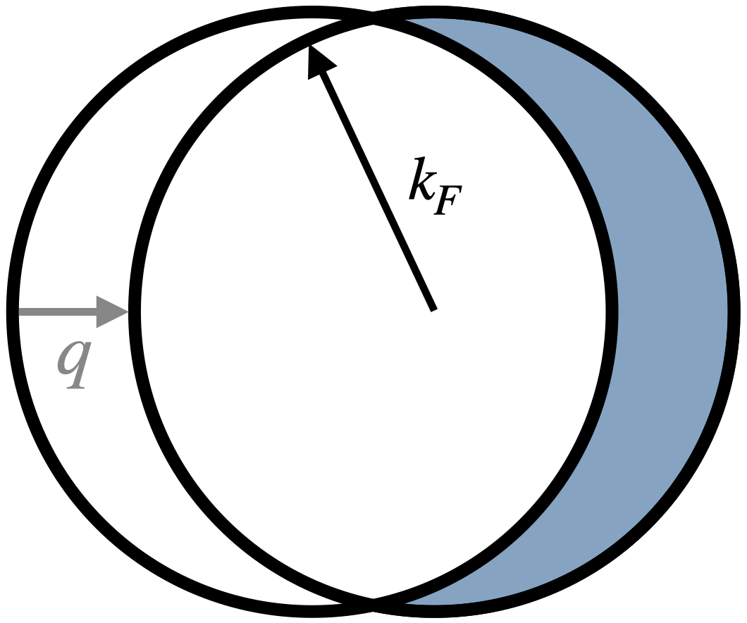
Figure 3: The geometric interpretation of the static structure factor $\Pi^{\tau\tau}(\tau\rightarrow 0,\bm{q})$, where the shaded area represents its value.

For a spherical fermi surface $\bm{k}_{F}(\theta)=k_{F}(\cos\theta,\sin\theta)$, we have $\bm{k}\times\partial_{\theta}\bm{k}_{F}(\theta)=\bm{k}\cdot\bm{k}_{F}(\theta)$, and accordingly

$$\Pi^{\tau\tau}(\tau\rightarrow 0,\bm{k})=\frac{1}{(2\pi)^{2}}\int\frac{\textrm{d}\omega}{2\pi}\int_{0}^{2\pi}\textrm{d}\theta\frac{k_{F}|\bm{k}|\cos\theta}{\mathtt{i}\omega-v_{F}|\bm{k}|\cos\theta}=\frac{k_{F}|\bm{k}|}{2\pi}\int_{0}^{2\pi}\frac{\textrm{d}\theta}{2\pi}\left(-\frac{|\cos\theta|}{2}\right)=-\frac{k_{F}|\bm{k}|}{2\pi^{2}}.$$ (63)

This exactly reproduces the free-fermion result in Eq. 2. It’s worth noting that one can introduce interactions that explicitly break the LU(1) symmetry, such as scattering between fermion modes from different patches. For instance, considering the RPA treatment of a local density-density interaction, we obtain the density response

$$\hat{\Pi}^{\tau\tau}(\mathtt{i}\omega,\bm{k})=\frac{\Pi^{\tau\tau}(\mathtt{i}\omega,\bm{k})}{1-u\Pi^{\tau\tau}(\mathtt{i}\omega,\bm{k})},$$ (64)

Here, $\Pi^{\tau\tau}(\mathtt{i}\omega,\bm{k})$ represents the free-fermion result from Eq. 31, and $u$ denotes a coupling constant. Consequently, the equal-time function becomes

$$\int\frac{\textrm{d}\omega}{2\pi}\hat{\Pi}^{\tau\tau}(\mathtt{i}\omega,\bm{k})=-\frac{k_{F}|\bm{k}|}{2\pi^{2}}\frac{\sqrt{2\tilde{u}+1}+2\tilde{u}\arctan(\sqrt{2\tilde{u}+1})}{(2\tilde{u}+1)^{3/2}},$$ (65)

where $\tilde{u}=u\mathscr{D}_{F}$ is rescaled by the density of states $\mathscr{D}_{F}=\frac{k_{F}}{2\pi v_{F}}$ at the fermi level. Also, note that in the problem of the half-filled Landau level, the Ward identity (Eq. 58) needs modification due to the presence of an emergent gauge field [44]. Therefore, the geometric interpretation presented here should not conflict with the results in Sec. V.2.1.

Appendix B Coulomb Gauge and Response Theory

In this appendix, we introduce our convention about the response theory under the Coulomb gauge. For any rotationally invariant systems, the two-point function $\Pi^{\mu\nu}=\langle J^{\mu}J^{\nu}\rangle$ of conserved currents has the structure

$$\Pi^{\tau\tau}(k) =\frac{|\bm{k}|^{2}}{\omega^{2}}\Pi_{L}(\omega,|\bm{k}|),$$

$$\Pi^{\tau i}(k) =-\frac{k_{i}}{\omega}\Pi_{L}(\omega,|\bm{k}|)+\varepsilon^{ij}k_{j}\mathsf{H}(\omega,|\bm{k}|),$$

$$\Pi^{ij}(k) =\frac{k_{i}k_{j}}{|\bm{k}|^{2}}\Pi_{L}(\omega,|\bm{k}|)+\left(\delta^{ij}-\frac{k_{i}k_{j}}{|\bm{k}|^{2}}\right)\Pi_{T}(\omega,|\bm{k}|)+\omega\varepsilon^{ij}\mathsf{H}(\omega,|\bm{k}|),$$ (66)

where $\Pi_{L}$ and $\Pi_{T}$ represent the longitudinal and transverse components respectively, while $\mathsf{H}$ governs the Hall response. It is sometimes beneficial to decompose the spatial components of the background/gauge field into longitudinal and transverse components, expressed as $\bm{A}=\bm{A}_{L}+\bm{A}_{T}$ where

$$\bm{A}^{L} (k)=\mathcal{P}^{L}\bm{A}(k),\qquad\mathcal{P}_{ij}^{L}=\frac{k_{i}k_{j}}{|\bm{k}|^{2}},$$

$$\bm{A}^{T} (k)=\mathcal{P}^{T}\bm{A}(k),\qquad\mathcal{P}_{ij}^{T}=\delta_{ij}-\mathcal{P}_{ij}^{L}.$$ (67)

It is useful to introduce a scalar $A_{T}$ to represent the transverse fields $A_{i}^{T}$, which is defined by

$$A_{i}^{T}(k)=\frac{\varepsilon_{ij}k_{j}}{|\bm{k}|}A_{T}(k),\qquad A_{T}(k)=\frac{\varepsilon_{ij}k_{j}}{|\bm{k}|}A_{i}^{T}(k).$$ (68)

Under the Coulomb gauge $\bm{A}^{L}=0$, the response theory can expressed in the basis $(A_{\tau},A_{T})$

$$\mathcal{S}[A]=\int\frac{\textrm{d}^{3}k}{(2\pi)^{3}}\frac{-1}{2}(A_{\tau}(-k)\;A_{T}(-k))\left(\begin{array}[]{cc}\Pi^{\tau\tau}(k)&\mathsf{H}(k)|\bm{k}|\\ \mathsf{H}(k)|\bm{k}|&\Pi^{TT}(k)\end{array}\right)\left(\begin{array}[]{c}A_{\tau}(k)\\ A_{T}(k)\end{array}\right),$$ (73)

where $\Pi^{\tau\tau}(k)=\frac{|\bm{k}|^{2}}{\omega^{2}}\Pi_{L}(\omega,|\bm{k}|)$ and $\Pi^{TT}(k)=-\Pi_{T}(k)$. Here, $k=(\omega,\bm{k})$ is a collective notion of frequency and momentum. Notice that the Chern-Simons term is

$$\int\frac{-\mathtt{i}}{4\pi}A\wedge\textrm{d}A=\int\frac{\textrm{d}^{3}k}{(2\pi)^{3}}\frac{-1}{2}(A_{\tau}(-k)\;A_{T}(-k))\frac{|\bm{k}|}{2\pi}\left(\begin{array}[]{cc}0&1\\ 1&0\end{array}\right)\left(\begin{array}[]{c}A_{\tau}(k)\\ A_{T}(k)\end{array}\right).$$ (78)

Appendix C Ioffe-Larkin Rule

We investigate the response function of electrons using the parton theory described in Eq. 10. In the standard RPA approach, integrating out both fermionic and bosonic partons $f$ and $b$ leads to

$$\mathcal{S}=\int_{k}\frac{-\Pi_{f}^{\mu\nu}(k)}{2}(a_{\mu}(-k)+e_{f}A_{\mu}(-k))(a_{\nu}(k)+e_{f}A_{\nu}(k))+\frac{-\Pi_{b}^{\mu\nu}(k)}{2}(-a_{\mu}(-k)+e_{b}A_{\mu}(-k))(-a_{\nu}(k)+e_{b}A_{\nu}(k)).$$ (79)

To enforce gauge invariance, we integrate out the dynamical gauge fields $a_{\mu}$ at the RPA level. This yields the total response theory $\mathcal{L}=\int_{k}\frac{-1}{2}\Pi^{\mu\nu}(k)A_{\mu}(-k)A_{\nu}(k)$ with

$$\Pi =e_{f}^{2}\Pi_{f}+e_{b}^{2}\Pi_{b}-(e_{f}\Pi_{f}-e_{b}\Pi_{b})(\Pi_{f}+\Pi_{b})^{-1}(e_{f}\Pi_{f}-e_{b}\Pi_{b})$$

$$=e_{f}^{2}(\Pi_{f}-\Pi_{f}(\Pi_{f}+\Pi_{b})^{-1}\Pi_{f})+e_{b}^{2}(\Pi_{b}-(\Pi_{f}+\Pi_{b})^{-1}\Pi_{b})+e_{b}e_{f}(\Pi_{f}(\Pi_{f}+\Pi_{b})^{-1}\Pi_{b}+\Pi_{b}(\Pi_{f}+\Pi_{b})^{-1}\Pi_{f})$$

$$=(e_{f}+e_{b})^{2}\Pi_{f}(\Pi_{f}+\Pi_{b})^{-1}\Pi_{b}=\Pi_{f}(\Pi_{f}+\Pi_{b})^{-1}\Pi_{b},$$ (80)

where we have used $e_{f}+e_{b}=1$. Therefore, we find the Ioffe-Larkin decomposition rule

$$\Pi^{-1}=\Pi_{f}^{-1}+\Pi_{b}^{-1},$$ (81)

which is independent of the assignment $(e_{f},e_{b})$ of the global $\textrm{U}(1)$ charge.

Under the Coulomb gauge, the parton response functions $\Pi_{f}$ and $\Pi_{b}$ can be written as

$$\Pi_{f}=\left(\begin{array}[]{cc}\Pi_{f}^{\tau\tau}(k)&\mathsf{H}_{f}|\bm{k}|\\ \mathsf{H}_{f}|\bm{k}|&\Pi_{f}^{TT}(k)\end{array}\right),\qquad\Pi_{b}=\left(\begin{array}[]{cc}\Pi_{b}^{\tau\tau}(k)&\mathsf{H}_{b}|\bm{k}|\\ \mathsf{H}_{b}|\bm{k}|&\Pi_{b}^{TT}(k)\end{array}\right).$$ (82)

The Ioffe-Larkin rule Eq. 81 leads to the gauge-invariant response

$$\Pi^{\tau\tau} =\frac{\Pi_{f}^{\tau\tau}\det(\Pi_{b})+\Pi_{b}^{\tau\tau}\det(\Pi_{f})}{\det(\Pi_{f}+\Pi_{b})},$$

$$\Pi^{TT} =\frac{\Pi_{f}^{TT}\det(\Pi_{b})+\Pi_{b}^{TT}\det(\Pi_{f})}{\det(\Pi_{f}+\Pi_{b})},$$

$$\Pi^{\tau T} =\Pi^{T\tau}=|\bm{k}|\frac{\mathsf{H}_{f}\det(\Pi_{b})+\mathsf{H}_{b}\det(\Pi_{f})}{\det(\Pi_{f}+\Pi_{b})}.$$ (83)

For time-reversal invariant systems such that $\mathsf{H}_{f}=0$ and $\mathsf{H}_{b}=0$, one simply has

$$\Pi^{\tau\tau}=\frac{\Pi_{f}^{\tau\tau}\Pi_{b}^{\tau\tau}}{\Pi_{f}^{\tau\tau}+\Pi_{b}^{\tau\tau}},\qquad\Pi^{TT}=\frac{\Pi_{f}^{TT}\Pi_{b}^{TT}}{\Pi_{f}^{TT}+\Pi_{b}^{TT}},\qquad\Pi^{\tau T}=\Pi^{T\tau}=0.$$ (84)

Appendix D Dual Theories for CFL-FL Transition

We begin by establishing the duality relation between the vortex theory Eq. 11 (together with Eq. 27) and the critical theory Eq. 30. It is known that a single Dirac fermion enjoys the fermion-fermion duality [72, 71]

$$\bar{\psi}\not{\textrm{D}}_{A}\psi\quad\longleftrightarrow\quad\bar{\chi}\not{\textrm{D}}_{a}\chi-\frac{\mathtt{i}}{2\pi}a\textrm{d}b+\frac{\mathtt{i}2}{4\pi}b\textrm{d}b-\frac{\mathtt{i}}{2\pi}b\textrm{d}A+\frac{\mathtt{i}}{4\pi}A\textrm{d}A,$$ (85)

where each Dirac fermion is defined through the Pauli-Villars scheme with another heavy Dirac fermion in the UV. Upon integrating out the gauge field $b$, the resulting expression takes on the usual form found in the literature, albeit with incorrectly quantized topological terms

$$\bar{\psi}\not{\textrm{D}}_{A}\psi-\frac{1}{2}\frac{\mathtt{i}}{4\pi}A\textrm{d}A\quad\longleftrightarrow\quad\bar{\chi}\not{\textrm{D}}_{a}\chi-\frac{1}{2}\frac{\mathtt{i}}{4\pi}a\textrm{d}a-\frac{1}{2}\frac{\mathtt{i}}{2\pi}a\textrm{d}A.$$ (86)

Its time-reversal image yields yet another fermionic particle-vortex duality

$$\bar{\psi}\not{\textrm{D}}_{A}\psi-\frac{1}{2}\frac{\mathtt{i}}{4\pi}A\textrm{d}A\quad\longleftrightarrow\quad\bar{\chi}\not{\textrm{D}}_{a}\chi-\frac{1}{2}\frac{\mathtt{i}}{4\pi}a\textrm{d}a+\frac{1}{2}\frac{\mathtt{i}}{2\pi}a\textrm{d}A.$$ (87)

Let us apply the duality Eq. 87 to the two fermions in Eq. 27, subject to the constraint $\psi_{1}^{\dagger}\psi_{1}=\psi_{2}^{\dagger}\psi_{2}$

$$\bar{\chi}_{1}\not{\textrm{D}}_{\tilde{b}}\chi_{1}+\bar{\chi}_{2}\not{\textrm{D}}_{\tilde{c}}\chi_{2}-\frac{1}{2}\frac{\mathtt{i}}{4\pi}\tilde{b}\textrm{d}\tilde{b}-\frac{1}{2}\frac{\mathtt{i}}{4\pi}\tilde{c}\textrm{d}\tilde{c}+\frac{\mathtt{i}}{2\pi}\tilde{a}\textrm{d}(A-a+\tilde{b}/2+\tilde{c}/2)+\frac{\mathtt{i}}{4\pi}\tilde{a}\textrm{d}\tilde{a}+\frac{\mathtt{i}}{2\pi}\lambda\textrm{d}(\tilde{b}-\tilde{c}),$$ (88)

where the fluxes of $\tilde{b}$ and $\tilde{c}$ represent the densities of $\psi_{1}$ and $\psi_{2}$, and $\lambda$ serves as a Lagrangian multiplier. After integrating out both $\lambda$ and $\tilde{a}$, we find that (when $\psi_{1}^{\dagger}\psi_{1}=\psi_{2}^{\dagger}\psi_{2}$)

$$\sum_{I=1}^{2}\bar{\psi}_{I}\not{\textrm{D}}_{\tilde{a}}\psi_{I}+\frac{\mathtt{i}}{2\pi}\tilde{a}\textrm{d}(A-a)\quad\longleftrightarrow\quad\sum_{I=1}^{2}\bar{\chi}_{I}\not{\textrm{D}}_{\tilde{b}}\chi_{I}-\frac{2\mathtt{i}}{4\pi}\tilde{b}\textrm{d}\tilde{b}-\frac{\mathtt{i}}{2\pi}\tilde{b}\textrm{d}(A-a)-\frac{\mathtt{i}}{4\pi}(A-a)\textrm{d}(A-a).$$ (89)

Together with the fermi-surface sector described by $\mathcal{L}_{\textrm{FS}}[f,a]$, we find Eq. 11 (together with Eq. 27) and Eq. 30 are indeed related by the fermionic particle-vortex duality [72, 71].

In view of the abelian duality web [72], there are other formulations of the critical theory as well. For a single Dirac fermion, there is a fermion-boson particle-vortex duality

$$\bar{\psi}\not{\textrm{D}}_{A}\psi\quad\longleftrightarrow\quad|\textrm{D}_{a}\varphi|^{2}+|\varphi|^{4}-\frac{\mathtt{i}}{4\pi}a\textrm{d}a-\frac{\mathtt{i}}{2\pi}a\textrm{d}A.$$ (90)

Using Eq. 90, we can express the dual theory of $\bar{\psi}_{1}\not{\textrm{D}}_{\tilde{a}}\psi_{1}+\bar{\psi}_{2}\not{\textrm{D}}_{\tilde{a}}\psi_{2}-\frac{\mathtt{i}}{2\pi}\tilde{a}\textrm{d}a$ as follows

$$|\textrm{D}_{\tilde{b}}\varphi_{1}|^{2}+|\varphi_{1}|^{4}+|\textrm{D}_{\tilde{c}}\varphi_{2}|^{2}+|\varphi_{2}|^{4}-\frac{\mathtt{i}}{4\pi}\tilde{b}\textrm{d}\tilde{b}-\frac{\mathtt{i}}{4\pi}\tilde{c}\textrm{d}\tilde{c}-\frac{\mathtt{i}}{2\pi}\tilde{a}\textrm{d}(a+\tilde{b}+\tilde{c}).$$ (91)

Integrating out $\tilde{a}$ imposes the constraint $\tilde{c}=-a-\tilde{b}$, leading to the bosonic dual theory for the CFL-FL transition

$$\mathcal{L}=\mathcal{L}_{\textrm{FS}}[f,a+A]+|\textrm{D}_{\tilde{b}}\varphi_{1}|^{2}+|\varphi_{1}|^{4}+|\textrm{D}_{-a-\tilde{b}}\varphi_{2}|^{2}+|\varphi_{2}|^{4}-\frac{2\mathtt{i}}{4\pi}\tilde{b}\textrm{d}\tilde{b}-\frac{\mathtt{i}}{2\pi}\tilde{b}\textrm{d}a-\frac{\mathtt{i}}{4\pi}a\textrm{d}a.$$ (92)

The phase transition is driven by the simultaneous condensation of $\varphi_{1}$ and $\varphi_{2}$.

In addition, several other dual critical theories based on level-rank dualities have been reviewed in Ref. [55].

Appendix E Static Structure Factor of Critical Fermi Surfaces

In this appendix, we provide technical details regarding the evaluation of integrals for the static structure factors, as expressed by Eq. 38 and Eq. 42, at the quantum critical points. If we naively consider the small-$\bm{k}$ expansion of the integrand before doing the integral, the leading-order term can integrated analytically, resulting in

$$\Pi^{\tau\tau}(\tau\rightarrow 0,\bm{k})\approx\int\frac{\textrm{d}\omega}{2\pi}\frac{-|\bm{k}|^{2}k_{F}v_{F}(k_{F}v_{F}\sigma_{xx}^{b}+4\pi\omega(\sigma_{xx}^{b})^{2}-4\pi\omega(\sigma_{xy}^{b})^{2})}{\omega(k_{F}v_{F}+4\pi\omega\sigma_{xx}^{b}){}^{2}-16\pi^{2}\omega^{3}(\sigma_{xy}^{b})^{2}}=-\frac{\sigma_{xx}^{b}}{\pi}|\bm{k}|^{2}\log(1/|\bm{k}|)+\ldots.$$ (93)

Here, a logarithmic divergence arises from the $\omega$-integral, leading to the factor $\log(1/|\bm{k}|)$ due to the identical scaling of $\omega$ and $\bm{k}$ at the critical point. The naive analytical calculation of Eq. 42 proceeds in a similar manner and is a special case of Eq. 93 with $\sigma_{xy}=0$.

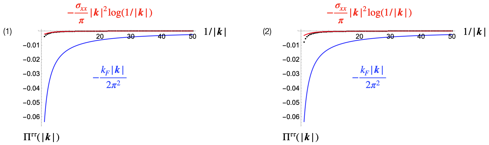
Figure 4: (1) The numerical result (in black) of the static structure factor given by Eq. 38 at the CFL-FL Transition, where $k_{F}=\sqrt{2\pi}$, $v_{F}=0.25$, and $\sigma_{xx}=-\sigma_{xy}=1/(8\pi)$; (2) The numerical result (in black) of the static structure factor given by Eq. 42 at the Mott Transition, where $k_{F}=\sqrt{2\pi}$, $v_{F}=0.25$, and $\sigma_{xx}=0.355155/(2\pi)$. The numerical results are compared to the CFT-like scaling (in red) and that of ordinary fermi surfaces (in blue).

To confirm the final result in Eq. 93, we also numerically evaluated the integrals using the exact expressions from Eq. 38 and Eq. 42, with the results presented in FIG. 4. In these numerical calculations, the value of $k_{F}$ is determined by the Luttinger theorem $V_{\textrm{FS}}/(2\pi)^{2}=1/2$ at half-filling , where the fermi-surface volume is given by $V_{\textrm{FS}}=\pi k_{F}^{2}$. We use a small value of $v_{F}$ for estimations. For the chargon conductivity $\sigma_{xx}^{b}$ at the Mott transition, we adopt the critical conductivity at the XY transition from conformal bootstrap [92]. For chargons at the CFL-FL transition, as a very crude estimation, we assume the universal transverse and Hall resistivities $\rho_{xx}^{b},\rho_{xy}^{b}$ are both around $4\pi$ [55]. In both cases, the numerical results agree well with the analytical expressions at small-$\bm{k}$, confirming the expectation that the static structure factor of critical fermi surfaces behaves in a CFT-like manner and deviates from that of ordinary fermi surfaces.

Appendix F Non-Linear Bosonization

In this Appendix, we offer a brief introduction to non-linear bosonization [46] of fermi liquids from the perspective of coherent-state construction. For any fermionic systems with translation symmetry, we can introduce the fermion bilinear operator

$$\mathbbm{t}(\bm{x},\bm{k})=\int_{\bm{q}}c_{\bm{k}-\frac{\bm{q}}{2}}^{\dagger}c_{\bm{k}+\frac{\bm{q}}{2}}e^{\mathtt{i}\bm{q}\cdot\bm{x}},$$ (94)

where $c$ is the gauge-invariant election operator. It generates an infinite-dimensional Lie algebra

$$[\mathbbm{t}(\xi),\mathbbm{t}(\eta)]=-2\mathtt{i}\sin\left(\frac{\partial_{\xi}\curlywedge\partial_{\eta}}{2}\right)\delta^{2d}(\xi-\eta)\mathbbm{t}(\xi),$$ (95)

where $\xi=(\bm{x},\bm{k})$ is a coordinate in the $2d$-dimensional phase space, and the antisymmetric product $\curlywedge$ is defined by $\xi\curlywedge\eta=\bm{\xi}^{x}\cdot\bm{\eta}^{p}-\bm{\xi}^{p}\cdot\bm{\eta}^{x}$. When $d=1$, this algebra is commonly known as the $W_{\infty}$ algebra. In higher dimensions, we refer to it as the particle-hole algebra. In the context of condensed matter systems, we assume that the phase space is compactified, with the momentum vector $\bm{k}$ living on the Brillouin zone which is a $d$-dimensional torus. The first observation is that fermi liquids realize a condensation of the Lie-algebra generator $\mathbbm{t}$

$$F_{0}(\bm{x},\bm{k})\overset{\textrm{df}}{=}\langle\textrm{FS}|\mathbbm{t}(\bm{x},\bm{k})|\textrm{FS}\rangle=\Theta(\epsilon_{F}-\epsilon_{\bm{k}}),$$ (96)

where $|\textrm{FS}\rangle=\prod_{\epsilon_{\bm{k}}\leq\epsilon_{F}}c_{\bm{k}}^{\dagger}|0\rangle$ is the fermi surface (FS) ground state. This is just the distribution function $F_{0}(\bm{x},\bm{k})$ that describes the shape of FS. This is analogous to magnetic orders that realize the condensation of fermion bilinears $\langle c^{\dagger}\vec{\sigma}c\rangle$ where $\vec{\sigma}$ are Pauli matrices.

The fluctuations of the condensation $\langle\mathbbm{t}\rangle$ are systematically described by nonlinear bosonization [46]. Given the symmetry group generated by the Lie algebra Eq. 95, one can introduce the coherent state

$$|\phi\rangle=\exp\left(\mathtt{i}\int_{\bm{x},\bm{k}}\phi(\bm{x},\bm{k})\mathbbm{t}(\bm{x},\bm{k})\right)|\textrm{FS}\rangle,$$ (97)

where $\phi(\bm{x},\bm{k})$ is a bosonic variable in phase space. The distribution function dressed by fluctuations is then

$$F(\bm{x},\bm{k})\overset{\textrm{df}}{=}\langle\phi|\mathbbm{t}(\bm{x},\bm{k})|\phi\rangle.$$ (98)

The quantization of FS fluctuations is given by the coherent-state path integral

$$\mathcal{Z}=\int\mathcal{D}[\phi]e^{-\mathcal{S}[\phi]},\qquad\mathcal{S}[\phi]=\int\textrm{d}\tau\langle\phi|\partial_{\tau}+H|\phi\rangle.$$ (99)

which can be unpacked order by order in terms of the boson $\phi$. In practical calculations [46], it is useful to consider a truncation of the algebra Eq. 95 using the separation of energy scales $\partial_{x}\partial_{k}\sim q/k_{F}\ll 1$, where $q$ is the low-energy relative momentum of particle-hole pairs. Another simplification comes from the redundancy in $\phi(\bm{x},\bm{k})$ due to the group generated by Eq. 95 being partially broken by the FS ground state. The FS fluctuations are sufficiently described by $\phi(\bm{x},\bm{k}_{F})$ where $\bm{k}_{F}$ labels points on the FS manifold [46]. The leading-order Gaussian part reproduces the well-known result based on patch assumptions

$$\mathcal{S}=\frac{1}{4\pi}\int_{\bm{k}_{F}\in\textrm{FS}}\int_{\tau,\bm{x}}(\hat{\bm{v}}_{F}\cdot\partial_{\bm{x}}\phi)(\mathtt{i}\partial_{\tau}\phi+\bm{v}_{F}\cdot\partial_{\bm{x}}\phi),$$ (100)

where $\bm{v}_{F}$ is the fermi velocity and $\hat{\bm{v}}_{F}$ denotes its direction. In other words, one has a chiral Luttinger liquid on each patch of the FS in the direction $\hat{\bm{v}}_{F}$. In the full action Eq. 99, different patches are allowed to talk to each other. Namely, the third-order term in $\phi$ contains the gradient $\partial_{\bm{k}_{F}}\phi$ along the FS, and therefore couples the nearest neighbor patches. For a more detailed analysis of the higher-order terms in the calculation, interested readers may consult Ref. [46]. It is worth noting that the procedure we have outlined here has parallels with the derivation of the non-linear sigma model for magnetic orders using spin coherent-state path integral methods. (see e.g. [93] for a textbook treatment).

References

- Laflorencie [2016] N. Laflorencie, Quantum entanglement in condensed matter systems, Physics Reports 646, 1 (2016).
- Wen [2017] X.-G. Wen, Colloquium: Zoo of quantum-topological phases of matter, Reviews of Modern Physics 89, 041004 (2017).
- Klich et al. [2006] I. Klich, G. Refael, and A. Silva, Measuring entanglement entropies in many-body systems, Physical Review A 74, 032306 (2006).
- Klich and Levitov [2009] I. Klich and L. Levitov, Quantum noise as an entanglement meter, Physical Review Letters 102, 100502 (2009).
- Hsu et al. [2009] B. Hsu, E. Grosfeld, and E. Fradkin, Quantum noise and entanglement generated by a local quantum quench, Physical Review B 80, 235412 (2009).
- Song et al. [2010] H. F. Song, S. Rachel, and K. Le Hur, General relation between entanglement and fluctuations in one dimension, Physical Review B 82, 012405 (2010).
- Song et al. [2011a] H. F. Song, N. Laflorencie, S. Rachel, and K. Le Hur, Entanglement entropy of the two-dimensional heisenberg antiferromagnet, Physical Review B 83, 224410 (2011a).
- Song et al. [2012] H. F. Song, S. Rachel, C. Flindt, I. Klich, N. Laflorencie, and K. Le Hur, Bipartite fluctuations as a probe of many-body entanglement, Physical Review B 85, 035409 (2012).
- Calabrese et al. [2012] P. Calabrese, M. Mintchev, and E. Vicari, Exact relations between particle fluctuations and entanglement in fermi gases, Europhysics Letters 98, 20003 (2012).
- Petrescu et al. [2014] A. Petrescu, H. F. Song, S. Rachel, Z. Ristivojevic, C. Flindt, N. Laflorencie, I. Klich, N. Regnault, and K. Le Hur, Fluctuations and entanglement spectrum in quantum Hall states, Journal of Statistical Mechanics: Theory and Experiment 2014, P10005 (2014).
- Song et al. [2011b] H. F. Song, C. Flindt, S. Rachel, I. Klich, and K. Le Hur, Entanglement entropy from charge statistics: Exact relations for noninteracting many-body systems, Physical Review B 83, 161408 (2011b).
- Frérot and Roscilde [2015] I. Frérot and T. Roscilde, Area law and its violation: A microscopic inspection into the structure of entanglement and fluctuations, Physical Review B 92, 115129 (2015).
- Rachel et al. [2012] S. Rachel, N. Laflorencie, H. F. Song, and K. Le Hur, Detecting quantum critical points using bipartite fluctuations, Physical Review Letters 108, 116401 (2012).
- Nussinov and Ortiz [2009] Z. Nussinov and G. Ortiz, A symmetry principle for topological quantum order, Annals of Physics 324, 977 (2009).
- Gaiotto et al. [2015] D. Gaiotto, A. Kapustin, N. Seiberg, and B. Willett, Generalized global symmetries, Journal of High Energy Physics 2015, 1 (2015).
- McGreevy [2023] J. McGreevy, Generalized symmetries in condensed matter, Annual Review of Condensed Matter Physics 14, 57 (2023).
- Cordova et al. [2022] C. Cordova, T. T. Dumitrescu, K. Intriligator, and S.-H. Shao, Snowmass white paper: Generalized symmetries in quantum field theory and beyond, arXiv preprint arXiv:2205.09545 (2022).
- Wu et al. [2021] X.-C. Wu, C.-M. Jian, and C. Xu, Universal features of higher-form symmetries at phase transitions, SciPost Physics 11, 033 (2021).
- Wang et al. [2021] Y.-C. Wang, M. Cheng, and Z. Y. Meng, Scaling of the disorder operator at quantum criticality, Physical Review B 104, L081109 (2021).
- Estienne et al. [2022] B. Estienne, J.-M. Stéphan, and W. Witczak-Krempa, Cornering the universal shape of fluctuations, Nature Communications 13, 287 (2022).
- Wang et al. [2022] Y.-C. Wang, N. Ma, M. Cheng, and Z. Y. Meng, Scaling of the disorder operator at deconfined quantum criticality, SciPost Physics 13, 123 (2022).
- Jiang et al. [2023] W. Jiang, B.-B. Chen, Z. H. Liu, J. Rong, F. F. Assaad, M. Cheng, K. Sun, and Z. Y. Meng, Many versus one: The disorder operator and entanglement entropy in fermionic quantum matter, SciPost Physics 15, 082 (2023).
- Liu et al. [2023a] Z. H. Liu, W. Jiang, B.-B. Chen, J. Rong, M. Cheng, K. Sun, Z. Y. Meng, and F. F. Assaad, Fermion disorder operator at Gross-Neveu and deconfined quantum criticalities, Physical Review Letters 130, 266501 (2023a).
- Liu et al. [2023b] Z. H. Liu, Y. Da Liao, G. Pan, W. Jiang, C.-M. Jian, Y.-Z. You, F. F. Assaad, Z. Y. Meng, and C. Xu, Disorder operator and Rényi entanglement entropy of symmetric mass generation, arXiv preprint arXiv:2308.07380 (2023b).
- Song et al. [2023a] M. Song, J. Zhao, L. Janssen, M. M. Scherer, and Z. Y. Meng, Deconfined quantum criticality lost, arXiv preprint arXiv:2307.02547 (2023a).
- Hertz [1976] J. A. Hertz, Quantum critical phenomena, Physical Review B 14, 1165 (1976).
- Millis [1993] A. J. Millis, Effect of a nonzero temperature on quantum critical points in itinerant fermion systems, Physical Review B 48, 7183 (1993).
- Löhneysen et al. [2007] H. v. Löhneysen, A. Rosch, M. Vojta, and P. Wölfle, Fermi-liquid instabilities at magnetic quantum phase transitions, Rev. Mod. Phys. 79, 1015 (2007).
- Nayak and Wilczek [1994a] C. Nayak and F. Wilczek, Non-fermi liquid fixed point in dimensions, Nuclear Physics B 417, 359 (1994a).
- Nayak and Wilczek [1994b] C. Nayak and F. Wilczek, Renormalization group approach to low temperature properties of a non-fermi liquid metal, Nuclear Physics B 430, 534 (1994b).
- Polchinski [1994] J. Polchinski, Low-energy dynamics of the spinon-gauge system, Nuclear Physics B 422, 617 (1994).
- Altshuler et al. [1994] B. Altshuler, L. Ioffe, and A. Millis, Low-energy properties of fermions with singular interactions, Physical Review B 50, 14048 (1994).
- Kim et al. [1994] Y. B. Kim, A. Furusaki, X.-G. Wen, and P. A. Lee, Gauge-invariant response functions of fermions coupled to a gauge field, Physical Review B 50, 17917 (1994).
- Lee [2009] S.-S. Lee, Low-energy effective theory of fermi surface coupled with gauge field in dimensions, Physical Review B 80, 165102 (2009).
- Mross et al. [2010] D. F. Mross, J. McGreevy, H. Liu, and T. Senthil, Controlled expansion for certain non-fermi-liquid metals, Physical Review B 82, 045121 (2010).
- Metlitski and Sachdev [2010] M. A. Metlitski and S. Sachdev, Quantum phase transitions of metals in two spatial dimensions. i. Ising-nematic order, Physical Review B 82, 075127 (2010).
- Dalidovich and Lee [2013] D. Dalidovich and S.-S. Lee, Perturbative non-fermi liquids from dimensional regularization, Physical Review B 88, 245106 (2013).
- Damia et al. [2019] J. A. Damia, S. Kachru, S. Raghu, and G. Torroba, Two-dimensional non-fermi-liquid metals: A solvable large- limit, Physical Review Letters 123, 096402 (2019).
- Maslov and Chubukov [2010] D. L. Maslov and A. V. Chubukov, Fermi liquid near Pomeranchuk quantum criticality, Physical Review B 81, 045110 (2010).
- Rech et al. [2006] J. Rech, C. Pépin, and A. V. Chubukov, Quantum critical behavior in itinerant electron systems: Eliashberg theory and instability of a ferromagnetic quantum critical point, Physical Review B 74, 195126 (2006).
- Ye et al. [2022] W. Ye, S.-S. Lee, and L. Zou, Ultraviolet-infrared mixing in marginal fermi liquids, Physical Review Letters 128, 106402 (2022).
- Esterlis et al. [2021] I. Esterlis, H. Guo, A. A. Patel, and S. Sachdev, Large- theory of critical fermi surfaces, Physical Review B 103, 235129 (2021).
- Guo et al. [2022] H. Guo, A. A. Patel, I. Esterlis, and S. Sachdev, Large- theory of critical fermi surfaces. ii. conductivity, Physical Review B 106, 115151 (2022).
- Else et al. [2021] D. V. Else, R. Thorngren, and T. Senthil, Non-fermi liquids as ersatz fermi liquids: general constraints on compressible metals, Physical Review X 11, 021005 (2021).
- Shi et al. [2022] Z. D. Shi, H. Goldman, D. V. Else, and T. Senthil, Gifts from anomalies: Exact results for landau phase transitions in metals, SciPost Physics 13, 102 (2022).
- Delacretaz et al. [2022] L. V. Delacretaz, Y.-H. Du, U. Mehta, and D. T. Son, Nonlinear bosonization of fermi surfaces: The method of coadjoint orbits, Physical Review Research 4, 033131 (2022).
- Florens and Georges [2004] S. Florens and A. Georges, Slave-rotor mean-field theories of strongly correlated systems and the mott transition in finite dimensions, Physical Review B 70, 035114 (2004).
- Lee and Lee [2005] S.-S. Lee and P. A. Lee, U(1) gauge theory of the hubbard model: Spin liquid states and possible application to , Physical Review Letters 95, 036403 (2005).
- Senthil [2008a] T. Senthil, Critical fermi surfaces and non-fermi liquid metals, Physical Review B 78, 035103 (2008a).
- Senthil [2008b] T. Senthil, Theory of a continuous mott transition in two dimensions, Physical Review B 78, 045109 (2008b).
- Li et al. [2021] T. Li, S. Jiang, L. Li, Y. Zhang, K. Kang, J. Zhu, K. Watanabe, T. Taniguchi, D. Chowdhury, L. Fu, et al., Continuous mott transition in semiconductor Moiré superlattices, Nature 597, 350 (2021).
- Note [1] See Ref. [94] for a discussion about the effects of disorder.
- Xu et al. [2022a] Y. Xu, X.-C. Wu, M. Ye, Z.-X. Luo, C.-M. Jian, and C. Xu, Interaction-driven metal-insulator transition with charge fractionalization, Physical Review X 12, 021067 (2022a).
- Barkeshli and McGreevy [2012] M. Barkeshli and J. McGreevy, Continuous transitions between composite fermi liquid and landau fermi liquid: A route to fractionalized mott insulators, Physical Review B 86, 075136 (2012).
- Song et al. [2023b] X.-Y. Song, Y.-H. Zhang, and T. Senthil, Phase transitions out of quantum Hall states in Moiré TMD bilayers, arXiv preprint arXiv:2308.10903 (2023b).
- Note [2] The existence of composite fermi liquids at 1/2 and 1/4 fillings in twisted is supported by Ref. [77, 78].
- Poland et al. [2019] D. Poland, S. Rychkov, and A. Vichi, The conformal bootstrap: theory, numerical techniques, and applications, Reviews of Modern Physics 91, 015002 (2019).
- Song et al. [2023c] M. Song, J. Zhao, Z. Y. Meng, C. Xu, and M. Cheng, Extracting subleading corrections in entanglement entropy at quantum phase transitions, arXiv preprint arXiv:2312.13498 (2023c).
- Wolf [2006] M. M. Wolf, Violation of the entropic area law for fermions, Physical Review Letters 96, 010404 (2006).
- Gioev and Klich [2006] D. Gioev and I. Klich, Entanglement entropy of fermions in any dimension and the Widom conjecture, Physical Review Letters 96, 100503 (2006).
- Ding et al. [2012] W. Ding, A. Seidel, and K. Yang, Entanglement entropy of fermi liquids via multidimensional bosonization, Physical Review X 2, 011012 (2012).
- Swingle [2010] B. Swingle, Entanglement entropy and the fermi surface, Physical Review Letters 105, 050502 (2010).
- Note [3] Private discussion with Prashant Kumar.
- Note [4] We use a different notation for critical fermi surfaces to distinguish it from used in CFTs.
- Barkeshli and McGreevy [2014] M. Barkeshli and J. McGreevy, Continuous transition between fractional quantum Hall and superfluid states, Physical Review B 89, 235116 (2014).
- Musser et al. [2022] S. Musser, T. Senthil, and D. Chowdhury, Theory of a continuous bandwidth-tuned Wigner-Mott transition, Physical Review B 106, 155145 (2022).
- Halperin et al. [1993] B. I. Halperin, P. A. Lee, and N. Read, Theory of the half-filled landau level, Physical Review B 47, 7312 (1993).
- Lee and Nagaosa [1992] P. A. Lee and N. Nagaosa, Gauge theory of the normal state of high- superconductors, Physical Review B 46, 5621 (1992).
- Frohlich et al. [1995] J. Frohlich, R. Gotschmann, and P. Marchetti, Bosonization of fermi systems in arbitrary dimension in terms of gauge forms, Journal of Physics A: Mathematical and General 28, 1169 (1995).
- Fröhlich et al. [1995] J. Fröhlich, R. Götschmann, and P. Marchetti, The effective gauge field action of a system of non-relativistic electrons, Communications in mathematical physics 173, 417 (1995).
- Son [2015] D. T. Son, Is the composite fermion a Dirac particle?, Physical Review X 5, 031027 (2015).
- Senthil et al. [2019] T. Senthil, D. T. Son, C. Wang, and C. Xu, Duality between quantum critical points, Physics Reports 827, 1 (2019).
- Girvin et al. [1985] S. Girvin, A. MacDonald, and P. Platzman, Collective-excitation gap in the fractional quantum Hall effect, Physical Review Letters 54, 581 (1985).
- Girvin et al. [1986] S. Girvin, A. MacDonald, and P. Platzman, Magneto-roton theory of collective excitations in the fractional quantum Hall effect, Physical Review B 33, 2481 (1986).
- Read [1998] N. Read, Lowest-landau-level theory of the quantum Hall effect: The fermi-liquid-like state of bosons at filling factor one, Physical Review B 58, 16262 (1998).
- Geraedts et al. [2016] S. D. Geraedts, M. P. Zaletel, R. S. Mong, M. A. Metlitski, A. Vishwanath, and O. I. Motrunich, The half-filled landau level: The case for Dirac composite fermions, Science 352, 197 (2016).
- Dong et al. [2023] J. Dong, J. Wang, P. J. Ledwith, A. Vishwanath, and D. E. Parker, Composite fermi liquid at zero magnetic field in twisted , Physical Review Letters 131, 136502 (2023).
- Goldman et al. [2023] H. Goldman, A. P. Reddy, N. Paul, and L. Fu, Zero-field composite fermi liquid in twisted semiconductor bilayers, Physical Review Letters 131, 136501 (2023).
- Note [5] In terms of space-time components, the response function has the form .
- Furukawa et al. [2018] T. Furukawa, K. Kobashi, Y. Kurosaki, K. Miyagawa, and K. Kanoda, Quasi-continuous transition from a fermi liquid to a spin liquid in -, Nature communications 9, 307 (2018).
- Zou and Chowdhury [2020] L. Zou and D. Chowdhury, Deconfined metallic quantum criticality: A gauge-theoretic approach, Physical Review Research 2, 023344 (2020).
- Lieb et al. [1961] E. Lieb, T. Schultz, and D. Mattis, Two soluble models of an antiferromagnetic chain, Annals of Physics 16, 407 (1961).
- Hastings [2004] M. B. Hastings, Lieb-Schultz-Mattis in higher dimensions, Physical Review B 69, 104431 (2004).
- Shao et al. [2015] J. Shao, E.-A. Kim, F. Haldane, and E. H. Rezayi, Entanglement entropy of the = 1/2 composite fermion non-fermi liquid state, Physical Review Letters 114, 206402 (2015).
- Mishmash and Motrunich [2016] R. V. Mishmash and O. I. Motrunich, Entanglement entropy of composite fermi liquid states on the lattice: In support of the Widom formula, Physical Review B 94, 081110 (2016).
- Xu et al. [2022b] Y. Xu, X.-C. Wu, and C. Xu, Deconfined quantum critical point with nonlocality, Physical Review B 106, 155131 (2022b).
- Podolsky et al. [2009] D. Podolsky, A. Paramekanti, Y. B. Kim, and T. Senthil, Mott transition between a spin-liquid insulator and a metal in three dimensions, Physical Review Letters 102, 186401 (2009).
- Mross and Senthil [2011] D. F. Mross and T. Senthil, Decohering the fermi liquid: A dual approach to the mott transition, Physical Review B 84, 165126 (2011).
- Note [6] Kang-Le Cai and Meng Cheng, to appear.
- Lu et al. [2024] D.-C. Lu, J. Wang, and Y.-Z. You, Definition and classification of fermi surface anomalies, Physical Review B 109, 045123 (2024).
- Note [7] The Luttinger theorem, as it applies to the composite fermi liquid and the spinon fermi surface, is discussed in Ref. [44]. The more precise expressions are and , where represents the magnetic length and denotes the volume of the unit cell. Our purpose is to numerically verify the analytic result in Eq. 93. To this end, we set and for simplicity.
- Kos et al. [2015] F. Kos, D. Poland, D. Simmons-Duffin, and A. Vichi, Bootstrapping the archipelago, Journal of High Energy Physics 2015, 1 (2015).
- Fradkin [2013] E. Fradkin, Field theories of condensed matter physics (Cambridge University Press, 2013).
- Kim et al. [2023] S. Kim, T. Senthil, and D. Chowdhury, Continuous mott transition in Moiré semiconductors: Role of long-wavelength inhomogeneities, Physical Review Letters 130, 066301 (2023).