Pattern formation from Gauge/Gravity Duality

Abstract

In the framework of the AdS/CFT correspondence, we report a complex scalar field dynamics in a $2+1$ dimensional black hole background can provide a scheme to study the pattern formation process in $1+1$ dimensional reaction-diffusion systems. The patterns include plane wave, defect turbulence, phase turbulence, spatio-temporal intermittency where defect chaos coexists with stable plane wave, and coherent structures. A phase diagram is obtained by studying the linear instability of the plane wave solutions to determine the onset of the holographic version of the Benjamin-Feir instability near a supercritical Hopf bifurcation.

Motivation– As a remarkable result emerged from string theory, the duality between a classical gravity theory and a quantum field theory living on its boundary is called AdS/CFT correspondence, also known as Gauge/Gravity duality or holography[1, 2, 3]. The correspondence provides an unique method for studying a strongly coupled quantum many body system in equilibrium/nonequilibrium by solving the independent/time-dependent equations of motion in the dual classical gravity theory, and has shown great power and potential in condensed matter physics (AdS/CMT)[4, 5, 6, 7, 8]. Here we firstly exhibit that duality can also provide a dual gravitational description of non-equilibrium pattern formation dynamics.

To understand the mechanism of spontaneous pattern formation out of equilibrium in fluids, plasmas, cosmology, crystals solidifying from a melt, and so on is one of the fundamental questions in nonequilibrium physics[9, 10, 11, 12, 13, 14]. Rather than a physical system, pattern formation is also frequently observed in a chemistry or biology system[15, 16, 17]. In contrast to pattern formation within thermodynamic equilibrium which rooted in the minimization of (free) energy, patterns emerging in nonequilibrium systems can only be understood within a dynamical framework, even if the patterns of interest are time independent. More often than not, when a system is driven far from equilibrium, spatially uniform structures become unstable toward the growth of small perturbations, which leads to dynamics that amplify fluctuations and increase complexity. Late-time dynamics is dominated by the fastest-growing fluctuating modes, whose characteristic length and time scales determine the resulting spatiotemporal patterns, eventually stabilized by nonlinear and dissipative mechanisms[10]. In such a dynamical framework, dynamical instabilities and nonlinear mode coupling mechanisms are crucial for pattern formation [11]. Due to the advent of Gauge/Gravity duality and the high nonlinear properties of Einstein gravity theory, we found that the dynamics of a neutral scalar field living in a charged black hole can demonstrate immense kinds of pattern formation on the boundary that arise naturally and autonomously from a spatial homogeneous, uniform oscillating state, including spatial periodic plane wave, defect turbulence, phase turbulence, spatio-temporal intermittency where defect chaos coexists with stable plane wave, and coherent structures. This is the first realization of Turing patterns [18] in reactive-diffusion systems from black hole physics.

Model from holography– To introduce a gravity theory that accounts for pattern formation, we consider a ($d+1)$-dimensional anti–de Sitter (AdS_d+1) spacetime, the Reissner-Nordström (RN) black hole background with a neutral complex scalar field $\Psi$ living from the horizon of the black hole to the infinity. The RN black hole is a solution of the Einstein-Maxwell theory with negative cosmological constant $\Lambda=-d(d-1)/2\ell^{2}$,

$$\mathcal{L}=R-2\Lambda+\alpha F_{\mu\nu}F^{\mu\nu}.$$ (1)

We further focus on the $d=2$ case to study the pattern formation dynamics of a 1+1 dimensional system living on the boundary of the $AdS_{3}$ RN black hole, where

$$A_{t}=-\mu\ln z,\quad f=1-z^{2}+\frac{\mu^{2}}{2}z^{2}\ln z,$$ (2)

with temperature

$$T=\frac{1}{4\pi}\left(2-\frac{\mu^{2}}{2}\right).$$ (3)

In the Eddington coordinate, $dt\to dt+du/f$, the metric has the form

$$ds^{2}=\frac{\ell^{2}}{z^{2}}\left(-f(z)dt^{2}-2dtdz+dx^{2}\right).$$ (4)

In the background of the RN black hole, we consider a neutral scalar with it’s Lagrangian reads

$$\mathcal{L}_{\Psi}=\frac{1}{2\kappa\lambda}(-V_{M}(\Psi)-V_{K}(\Psi)).$$ (5)

One term of the the Lagrangian is the nonlinear Mexican hat potential

$$V_{M}=\frac{1}{4\ell^{2}}((1+i\beta)\Psi^{2}\Psi^{*2}+2\Psi\Psi^{*}m^{2}\ell^{2}),$$ (6)

and the other term is the kinetic energy term

$$V_{K}=\frac{1}{2}(\partial_{t}\Psi\partial^{t}\Psi^{*}+\partial_{z}\Psi\partial^{z}\Psi^{*}+(1+i\alpha)\partial_{x}\Psi\partial^{x}\Psi^{*}),$$ (7)

The equation of motion for the complex scalar field has the following form

$$(2z^{2}\partial_{t}\partial_{z}-z\partial_{t})\Psi=z^{2}(1+i\alpha)\partial_{x}^{2}\Psi-(1+i\beta)\Psi^{2}\Psi^{*}$$

$$+z^{2}\partial_{z}(f\partial_{z}\Psi)-zf\partial_{z}\Psi-m^{2}\Psi.$$ (8)

The asymptotic expansion of the field near the boundary are

$$\Psi\big{|}_{z=0}=\Psi^{-}z^{\triangle^{-}}+\Psi^{+}z^{\triangle^{+}},$$ (9)

where

$$\triangle^{\pm}=\frac{2\pm\sqrt{4+4m^{2}}}{2}.$$ (10)

Standard quantization is adopted on the boundary, where $\Psi^{-}$ can be regarded as the source of the operator in the boundary field theory and $\Psi^{+}$ can be regarded as the expected value of the scalar operators $\mathcal{O}$. Setting the source of the operator $\Psi^{-}$=0, one obtains a spontaneous symmetry-breaking state in this holographic setting when the temperature of the black hole below a critical value. By setting $\alpha=\beta=0$, this model was firstly proposed and studied in [19], which dual to a mean field second order phase transition with $U(1)$ symmetry broken by tunning the temperature of the RN black.

In this letter, we set the mass to $m^{2}=-0.99$, which is a little above the Breitenlohner-Freedman bound $-d^{2}/4$, the critical temperature is $T_{c}=0.0135$, corresponding to $\mu_{c}=1.90$. We will show that by tuning on $\alpha$ and $\beta$ in the symmetry broken phase, the system will demonstrate various pattern formations as observed in a one-dimensional reactive-diffusion system. Notice that the critical temperature of the model will not be affected by the nonlinear high order term with $\alpha$ and $\beta$, which can be throw out near the critical point when the scalar is tiny. We chose a typical symmetry broken state $T=0.294T_{c}$. The size of a one-dimensional reaction-diffusion system growing on the boundary is set to $L=500$. In order to solve the dynamic equation (8), the following numerical methods are necessary the Chebyshev spectral method is used in the $z$ direction, the Fourier spectral method is used in the $x$ direction. Specifically, the number of points in the $z$ direction and the $x$ direction is $n_{z}=30$ and $n_{x}=500$, respectively. The fourth-order Runge-Kutta method is used to simulate the evolution of the system in the time direction, and the time step is $h=0.01$.

Plane wave solution, Benjamin–Feir instability and phase diagram– After solving dynamic Eq. (8) by the fourth-order Runge-Kutta method from a zero $\Psi$ initial state with small fluctuations, we found that there are plane wave solutions in this holographic reaction-diffusion system which are related to the parameters $(\alpha,\beta,q)$ and take the form of

$$\Psi(z,t,x)=\psi(z)e^{i\omega t+iqx},$$ (11)

where $\psi(z)$ is a monotonically increasing function with respect to $z$. It should be emphasized that the solutions of the dynamic Eq. (8) is not always a plane wave solutions unless the ansatz Eq. (11) is adopted. Then we can obtain the Fourier transform form of the dynamic Eq. (8)

$$i\omega(2z^{2}\partial_{z}-z)\psi=-q^{2}z^{2}(1+i\alpha)\psi-(1+i\beta)\psi^{2}\psi^{*}$$

$$+z^{2}\partial_{z}(f\partial_{z}\psi)-zf\partial_{z}\psi-m^{2}\psi.$$ (12)

By the way, Eq. (12) can be easily solved by the Newton-Raphson iteration method. According to Eq. (9), the order parameter of the boundary field theory reads $\mathcal{O}=|\mathcal{O}|e^{i\omega t+iqx}$. $\mathcal{O}$ and $\omega$ are both related to parameters $(\alpha,\beta,q)$. Specifically, they are

$$|\mathcal{O}(\alpha,\beta,q)^{2}|=|\mathcal{O}_{0}(\beta)^{2}|-(0.0276+0.00219\alpha\beta)q^{2},$$ (13)

and

$$\omega(\alpha,\beta,q)=\omega_{0}(\beta)-(0.108\alpha-0.127\beta)q^{2},$$ (14)

where $|\mathcal{O}_{0}(\beta)^{2}|$ and $\omega_{0}(\beta)$ are defined at $q=0$, they are $|\mathcal{O}_{0}(\beta)^{2}|=0.00373+0.000190\beta^{2}$ and $\omega_{0}(\beta)=5.02|\mathcal{O}_{0}(\beta)^{2}|$. All the plane wave solutions obtained from Eq. (12) can be verified by the dynamic Eq. (8). However, the plane wave solutions may not be stable for all $\alpha$ and $\beta$, this can be studied by using the linear instability analysis.

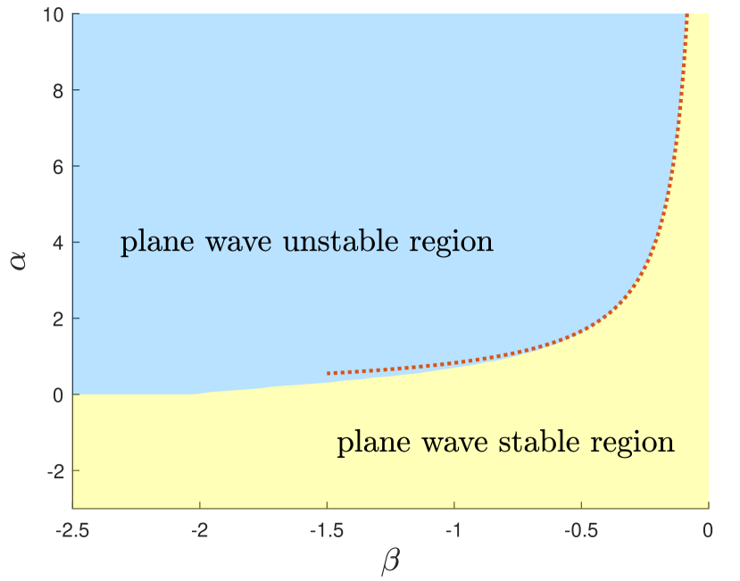
Figure 1: Holographic Benjamin-Feir-Newell (BF) line and phase diagram of the holographic reaction-diffusion system. The red fitting line is $\alpha=-0.828\beta^{-1}$.

In the background of plane wave solutions, the phase diagram of holographic reaction-diffusion systems can be obtained through the instability of the solutions. Like the usual linear instability analysis process, the plane wave solution with $q=0$, $\Psi=\Psi_{0}(z)e^{i\omega t}$ is disturbed by adding a small perturbation $\epsilon(t,z,x)=\delta_{1}(z)e^{\lambda t+ikx}+\delta^{*}_{2}(z)e^{\lambda^{*}t-ikx}$

$$\Psi=[\Psi_{0}+\epsilon(t,z,x)]e^{i\omega t}.$$ (15)

Substitute Eq. (15) to the dynamic Eq. (8) we get the first order perturbation equations for $\delta_{1}$ and $\delta_{2}$

$$\left\{\begin{aligned} &\hat{A}\delta_{1}+\hat{C}\delta_{2}=\lambda\hat{D}_{t}\delta_{1},\\ &\hat{A}^{*}\delta_{2}+\hat{C}^{*}\delta_{1}=\lambda\hat{D}_{t}^{*}\delta_{2}.\end{aligned}\right.$$ (16)

where $\hat{A}=z\left((1+i\alpha)k^{2}z-i\omega\right)+m^{2}+2(1+i\beta)\Phi_{0}\Phi_{0}^{*}+z\left(-z\partial_{z}f+f+2i\omega z\right)\partial_{z}-z^{2}f\partial_{z}^{2}$, $\hat{C}=(1+i\beta)\Psi_{0}^{2}$, $\hat{D}_{t}=z-2z^{2}\partial_{z}$. Solving the generalized eigenvalue Eq. (16) the growing rate $Re(\lambda(k))$ of the perturbation can be extracted, where $Re(\lambda(k))$ is the real part of the eigenvalue $\lambda(k)$. The zero $q$ plane wave solution will be destroyed by the growing perturbations if there are $Re(\lambda(k))>0$, corresponding to the linear unstable region in the phase diagram as shown in Fig.1. Four sample results of $Re(\lambda(k))$ for different combinations of $\alpha$ and $\beta$ are given in Fig. 4. If $Re(\lambda(k))\leq 0$, the plane wave solution is robust to the added perturbation, corresponding to the linear stable region in Fig.1. This is a holographic version of Benjamin–Feir instability, where deviations from a periodic waveform solution are reinforced by nonlinearity, leading to the generation of spectral-sidebands and the eventual breakup of the plane wave solution into a chaotic solution [20, 21].

Spatiotemporal Chaos– Now let us discuss behaviour of the solutions ofthe holographic model when the Benjamin-Feir-Newell criterion is violated. In particular beyond the BF instability line but close to the critical line in Fig.1 exhibits so-called phase turbulence regime. Phase turbulence is a state that $\mathcal{O}(x,t)=|\mathcal{O}|e^{i\theta}$ evolves irregularly, but with its modulus always fluctuates a bit near a constant value far from zero. While for the phase $\theta$, periodic boundary conditions enforce the winding number to be a constant of motion, fixed by the initial condition. As can be seen on Fig. 2, when $(\alpha,\beta)=(3,-0.65)$, this is a spatio-temporally chaotic state the amplitude of order parameter never reaches zero and remains saturated. Moreover, away from the BF line, for example $(\alpha,\beta)=(3,-1.5)$ the system exhibits spatio-temporally disordered regime called amplitude or defect turbulence. The behaviour in this region is characterised by defects, where the order parameter vanishes (see Fig. 2) . To obtain dynamics for the formation of chaos we begin with a zero $\Psi$ plus spatial noise of amplitude $h=10^{-3}$, admits the standard normal distribution.. Sure, we can also get the same results by beginning with the plane wave solution of the corresponding $\alpha$ and $\beta$ with spatial noise (not shown ). The linear instability analysis results of the plane wave solution shown in Fig. 4 confirmed the plane solution will finally enter a chaotic state after a long-time evolution.

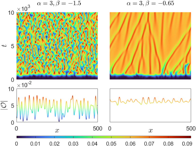
Figure 2: Configuration of $|\mathcal{O}(x,t)|$ for Defect turbulence (left) and phase turbulence (right) in the linear unstable region. The column below shows $|\mathcal{O}(x)|$ at $t=10000$.

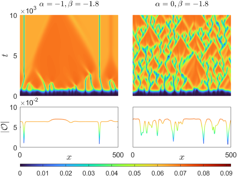
Figure 3: Configuration of $|\mathcal{O}(x,t)|$ for The moving hole-shock pair(left) and spatio-temporal intermittency (right).The column below shows $|\mathcal{O}(x)|$ at $t=10000$.

The spatio-tempora intermittency and Coherent structures in the plane wave stable region– Even in the regime where plane waves are stable, where the perturbation with finite $k$ will exponential decay as shown in Fig. 4, the linear stability of the plane wave solution Eq. (11) can not exclude the existence or coexistence of the other nontrivial solutions of Eq. (8). Below the Benjamin-Feir instability line, plane waves attract most initial conditions. However, using a suitably large and localized initial condition, spatio-temporally intermittent states, where defect chaos coexists with stable plane wave may appear. After a rather short time evolution, a typical intermittency regime solution consists of localized structures, separating lager regions of almost constant amplitude which are patches of stable plane wave solution emerges, as shown in Fig. 3 (right), when $(\alpha,\beta)=(0,-1.8)$. Fig. 3 (left) shows another typical nontrivial solution called sink solutions with Bekki-Nozaki holes [22], observed for $(\alpha,\beta)=(-1,-1.8)$. In this case, the spatial extension of the system is broken by irregular arrangements of stationary hole- and shock-like objects separated by turbulent dynamics. These structures asymptotically connect plane waves of different amplitude and wave number. Notice that the solution illustrated in Fig. 3 (left) are part of a family of solutions called coherent structures which are comprised of fixed spatial profiles that can vary through propagation and oscillation [23].

Discussion– We have shown that a simple 2+1 dimensional classic gravity theory shows many patterns that appear in the 1+1 dimensional systems on its boundary. By tuning the two parameters $\alpha$ and $\beta$ the plane wave solution will be unstable and finally the system will enter various patterns. This model provides a holographic simulation of the dynamics of generic spatially extended systems which undergoes a super-critical Hopf bifurcation from a stationary state to an oscillatory state. We also notice that the obtained patterns are very similar to the 1+1 dimension complex Gindzburg-Landau equation (CGLE)[10, 24, 25, 26, 27], the classic reductive perturbation method proved that any reaction-diffusion system that is close to this bifurcation can be deduced to the CGLE [28, 29]. With similarity we can refer the bulk theory to a holographic reaction-diffusion system. There are many extensions that we hope to consider elsewhere: (i) Extend the model to higher spatial dimensions. (ii) Try to derive the effective boundary field theory of the holographic model and compare it to the CGLE. (iii) Find the complete phase diagram and other possible coherent structures include sinks, fronts and shocks amongst others of the holographic model.

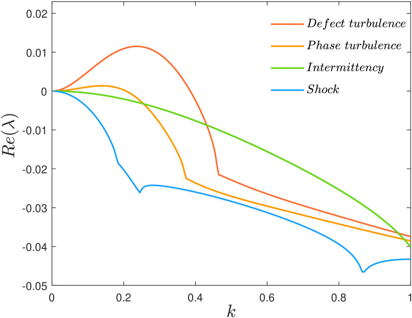
Figure 4: The real part of $\lambda$ (the growing rate of perturbation) versus $k$ in the background of plane wave solution, corresponding to the four situations shown in Fig. 2 and Fig. 3, respectively are defect turbulence($(\alpha,\beta)=(3,-1.5)$), phase turbulence($(\alpha,\beta)=(3,-0.65)$), moving hole-shock($(\alpha,\beta)=(-1,-1.8)$), and Spatio-temporal intermittency($(\alpha,\beta)=(0,-1.8)$).

Acknowledgements. H.B. Z. acknowledges the support by the National Natural Science Foundation of China (under Grants No. 12275233)

References

- Maldacena [1999] J. Maldacena, The large-n limit of superconformal field theories and supergravity, International Journal of Theoretical Physics 38, 1113 (1999).
- Gubser et al. [1998] S. Gubser, I. Klebanov, and A. Polyakov, Gauge theory correlators from non-critical string theory, Physics Letters B 428, 105 (1998).
- Witten [1998] E. Witten, Anti de sitter space and holography, Advances in Theoretical and Mathematical Physics 2, 253 (1998).
- Zaanen et al. [2015] J. Zaanen, Y. Liu, Y.-W. Sun, and K. Schalm, Holographic duality in condensed matter physics (Cambridge University Press, 2015).
- Ammon and Erdmenger [2015] M. Ammon and J. Erdmenger, Gauge/gravity duality: Foundations and applications (Cambridge University Press, 2015).
- Hartnoll et al. [2018] S. A. Hartnoll, A. Lucas, and S. Sachdev, Holographic quantum matter (MIT press, 2018).
- Zaanen [2021] J. Zaanen, Lectures on quantum supreme matter (2021).
- Liu and Sonner [2019] H. Liu and J. Sonner, Holographic systems far from equilibrium: a review, Reports on Progress in Physics 83, 016001 (2019).
- Cross and Greenside [2009] M. Cross and H. Greenside, Pattern Formation and Dynamics in Nonequilibrium Systems (Cambridge University Press, 2009).
- Cross and Hohenberg [1993] M. C. Cross and P. C. Hohenberg, Pattern formation outside of equilibrium, Rev. Mod. Phys. 65, 851 (1993).
- Gollub and Langer [1999a] J. P. Gollub and J. S. Langer, Pattern formation in nonequilibrium physics, Reviews of Modern Physics 71, S396 (1999a).
- Liddle and Lyth [2000] A. R. Liddle and D. H. Lyth, Frontmatter, in Cosmological Inflation and Large-Scale Structure (Cambridge University Press, 2000) pp. i–vi.
- Gollub and Langer [1999b] J. P. Gollub and J. S. Langer, Pattern formation in nonequilibrium physics, in More Things in Heaven and Earth: A Celebration of Physics at the Millennium, edited by B. Bederson (Springer New York, New York, NY, 1999) pp. 665–676.
- Mouritsen [1990] O. G. Mouritsen, Pattern Formation in Condensed Matter, International Journal of Modern Physics B 4, 1925 (1990).
- Maini et al. [1997] P. Maini, K. Painter, and H. P. Chau, Spatial pattern formation in chemical and biological systems, Journal of the Chemical Society, Faraday Transactions 93, 3601 (1997).
- Petrov et al. [1997] V. Petrov, Q. Ouyang, and H. L. Swinney, Resonant pattern formation in achemical system, Nature 388, 655 (1997).
- Turing [1952] A. M. Turing, The Chemical Basis of Morphogenesis, Philosophical Transactions of the Royal Society of London Series B 237, 37 (1952).
- Turing [1990] A. M. Turing, The chemical basis of morphogenesis, Bulletin of mathematical biology 52, 153 (1990).
- Iqbal et al. [2010] N. Iqbal, H. Liu, M. Mezei, and Q. Si, Quantum phase transitions in holographic models of magnetism and superconductors, Phys. Rev. D 82, 045002 (2010).
- Benjamin [1967] T. B. Benjamin, Instability of Periodic Wavetrains in Nonlinear Dispersive Systems, Proceedings of the Royal Society of London Series A 299, 59 (1967).
- Benjamin and Feir [1967] T. B. Benjamin and J. E. Feir, The disintegration of wave trains on deep water. Part 1. Theory, Journal of Fluid Mechanics 27, 417 (1967).
- Nozaki and Bekki [1984] K. Nozaki and N. Bekki, Exact solutions of the generalized ginzburg-landau equation, Journal of the Physical Society of Japan 53, 1581 (1984).
- van Saarloos and Hohenberg [1992] W. van Saarloos and P. Hohenberg, Fronts, pulses, sources and sinks in generalized complex ginzburg-landau equations, Physica D: Nonlinear Phenomena 56, 303 (1992).
- Aranson and Kramer [2002] I. S. Aranson and L. Kramer, The world of the complex ginzburg-landau equation, Rev. Mod. Phys. 74, 99 (2002).
- Bekki and Nozaki [1985] N. Bekki and K. Nozaki, Formations of spatial patterns and holes in the generalized ginzburg-landau equation, Physics Letters A 110, 133 (1985).
- Shraiman et al. [1992] B. Shraiman, A. Pumir, W. van Saarloos, P. Hohenberg, H. Chaté, and M. Holen, Spatiotemporal chaos in the one-dimensional complex ginzburg-landau equation, Physica D: Nonlinear Phenomena 57, 241 (1992).
- Chate [1994] H. Chate, Spatiotemporal intermittency regimes of the one-dimensional complex ginzburg-landau equation, Nonlinearity 7, 185 (1994).
- Kuramoto [1984] Y. Kuramoto, Chemical Oscillations, Waves, and Turbulence (Springer Berlin, Heidelberg, 1984).
- Nicolis [1995] G. Nicolis, Introduction to Nonlinear Science (Cambridge University Press, 1995).