Incoherent polariton dynamics and nonlinearities in organic light-emitting diodes
Abstract
Organic light-emitting diodes (OLEDs) have redefined lighting with their environment-friendliness and flexibility. However, only 25 % of the electronic states of fluorescent molecules can emit light upon electrical excitation, limiting the overall efficiency of OLEDs. Strong light-matter coupling, achieved by confining light within OLEDs using mirrors, generates polaritons—hybrid light-matter states—that could activate the remaining 75 % electronic states. Here, we show how different processes in such polariton OLEDs can be expected to change using a phenomenological quantum master equation model. We are especially interested in reverse inter-system crossing happening directly from the dark triplet states to the emitting lower polariton. We derive a simple expression for the enhancement factor of polaritonic RISC in the linear regime. In addition, we explore the extension of our model to higher dimensions and study some potential effects of strong coupling on nonlinear processes such as triplet-triplet annihilation.
I Introduction
Organic light-emitting diodes (OLEDs) offer several advantages over traditional lighting alternatives. One key aspect is their versatility in design and form; OLEDs are incredibly thin, lightweight, and flexible, allowing for innovative lighting solutions and high-definition displays [1]. However, due to spin statistics, electrical injection in molecular materials results in 25 % of the excitations to populate singlet electronic states, the rest 75 % populating triplets. Typically, singlets are favored due to their ability to undergo fluorescence, which is substantially faster compared to phosphorescence, thus reducing the likelihood of losses from exciton-exciton and exciton-polaron collisions [2, 3]. From the fundamental perspective, optical excitation is experimentally simpler and allows to create more singlets, but electrical excitation remains practical in real-life applications, e.g., OLEDs. Hence, 75 % of the created excitons are destined to become triplets, yet our aim should be to convert them into singlets or rapidly radiatively depopulate them [4, 5, 6].
In reverse inter-system crossing (RISC), excited triplet states can convert to singlet states via spin-orbit coupling and thermal activation [7]. Through molecular design, the energy landscape of organic materials can be manipulated to bring singlets and triplets closer in energy while maintaining high spin-orbit coupling, thereby enhancing RISC. However, an alternative approach exists, leveraging strong light-matter coupling phenomena to create polaritons—hybrid light-matter states with energy levels distinct from those of singlets and triplets [8, 9, 10]. It is an active research question whether this “artificial Stokes shift” can facilitate more efficient energy transfer from the triplet states, potentially bypassing the need for traditional molecular design and revolutionizing the field of organic optoelectronics [11, 12, 13, 14, 15, 16, 17, 18].
In Ref. [11], Erythrosine B was utilized to experimentally investigate the impact of polaritonic states on RISC, revealing a direct transition between molecular-centered and polaritonic states when bringing the lower polariton closer to the first-order triplet. However, the problem is much more nuanced. With TDAF, for example, enhanced RISC was not observed [12]. There have been contradictory results even with inverted lower polaritons; With DABNA-2, direct RISC from the triplets to the lower polariton (inverted below the triplets) was observed [13], but with 3DPA3CN it was not [14]. While theoretical explanations have been given [15], they appear separate, and a unified theory is still missing.
Theoretically, a common approach to this and other related problems is through quantum master equations [18, 19, 20, 21, 22, 23, 24]. While the existing models offer detailed insights into specific aspects of the system’s behavior, they are either too simplistic when omitting the abundance of other processes occurring in OLEDs or they suffer from computational complexity, making them impractical for large-scale simulations.
In this work, we develop a quantum master equation model that treats all the major (linear) processes occurring in polariton OLEDs as simple, incoherent quantum jumps. With our model, we can i) perform more detailed analysis on electrical excitation, often omitted in the literature, ii) obtain a simple expression for the RISC rate, and iii) see how these and all other processes behave as functions of , the coupling strength of light and matter, corresponding to bare film outside a cavity; To the best of our knowledge, no other model has simultaneously covered both the cavity and bare-film case. Our model is relatively simple, which allows for faster computations and easier interpretations. Furthermore, while the model only applies in the single-excitation subspace, we also discuss its extension to higher dimensions and how strong coupling could affect such processes as singlet-singlet and triplet-triplet annihilation. In general, our work helps to better understand the rich dynamics occurring in polariton OLEDs and paves the way for more advanced hybrid light-matter technologies.
This article is structured as follows. In Sec. II, we describe our model in full detail and solve it under steady-state conditions. In Sec. III, we derive the enhancement factor of RISC. Extending the model to higher dimensions and intermolecular processes are briefly discussed in Sec. IV, and Sec. V concludes the paper.
II The model
II.1 Hamiltonian and main assumptions
We consider a system of identical organic molecules carrying a single exciton coupled to a single cavity mode. Taking singlets (), triplets (), and the surrounding phonon bath into account, we can describe the system with the Holstein-Tavis-Cummings Hamiltonian [21, 22]
| (1) |
where we have used the rotating-wave approximation and assumed dominance of the singlet-cavity mode coupling. Here, and are the creation operators of a photon with the energy and a phonon with the energy at molecular site , respectively. and are the corresponding annihilation operators. Global ground state is denoted by , and —defined by —is the light-matter coupling strength.
The transition dipole moment of triplets is typically negligible for non-phosphorescent molecules [15], which allows us to omit triplet-cavity mode interactions. The - couplings, in turn, can be omitted if the energy gap between the lowest-order singlet and triplet is large enough, which it is, e.g., with TDAF [12]. Finally, phonon-couplings can be neglected due to polaritons being able to decouple electronic and vibrational degrees of freedom [22]. And in the absence of such explicit decoupling, phonons just suppress the effective light-matter coupling strength [25]. That is, should be understood as a function of the Huang-Rhys factor with .
Diagonalizing the Hamiltonian (1), we arrive at the trivial eigenstates in the triplet manifold and the following eigenstates in the singlet-cavity mode manifold,
| (2) | ||||
| (3) | ||||
| (4) |
is the upper polariton (UP) and the lower polariton (LP), whereas constitutes the non-emitting exciton reservoir. In the above expressions, () denotes the th molecule carrying a singlet (triplet) exciton, while the rest of the molecules are in their electronic ground states. The matching eigenvalues are
| (5) |
for the polaritons ( for UP and for LP) and for the dark states.
It is straightforward to show that the parameters and satisfy
| (6) | ||||
| (7) |
The weights and are known as the Hopfield coefficients [26], and they will play a crucial role in what follows. In particular, it is important to keep in mind how these quantities behave when , as this corresponds to the bare-film case: , , , and .
II.2 GKSL master equation and jump operators
No quantum system (like an exciton or cavity mode) can be truly isolated from their environment. The Gorini-Kossakowski-Sudarshan-Lindblad (GKSL) master equation is a convenient tool to study the dynamics of such open quantum systems. Denoting the open-system state by , the GKSL master equation reads [27]
| (8) |
The commutator is responsible for the unitary dynamics of the system, while the sum over jump operators —having units of —gives the non-unitary dynamics emerging from the environment interactions. The anti-commutator appearing in Eq. (8) is defined as .

Eq. (8) is the main tool of this paper. That is, describes the joint state of singlets, triplets, and cavity mode—phonons are counted in the environment. All the processes are schematically visualized in Fig. 1, and we will present the corresponding jump operators in the following subsections. Focusing on the non-unitary part of Eq. (8) is a valid simplification due to the sheer size of the system; With molecules, coherences typically get washed out due to interactions with the environment, leading to the dominance of incoherent processes.
II.2.1 Electrical excitation
We describe electrical excitation with the operators
| (9) | ||||
| (10) |
i.e., electronic states and are created at the molecular sites with the site-dependent rates and . Here, we have defined with triplets weighted threefold over singlets. That is, we treat the different spin configurations of triplets in a degenerate fashion. Furthermore, the parameter (the probability of phase flip) controls the singlet-triplet coherences; With , there are none.
From a simplistic point of view, the rate of electrical excitation depends on only two factors: How many electrons and holes per second and ground-state site are injected to the system and where the available sites are located. The number of electrons per second is given by the ratio of current and elementary charge, , which we can also write in terms of the current density and the device’s active area as . If there are less holes than electrons, we need to multiply this by the electron-hole balance ratio [28]. Taking the available sites into account, we get ; The more available sites there are, the less probable it is for the specific site to get excited. With the picture becomes nonphysical, but this can be disregarded in our case since we are dealing with one exciton and molecules.
Then, say the electrons and holes move at the drift velocities and , respectively, and once they meet somewhere between the electrodes, they combine to form excitons in the characteristic recombination time [29]. Here, is the width of the recombination zone and is the effective diffusion coefficient of electrons and holes. If we assume that no excitons can be formed outside the recombination zone, we finally get the pumping rate
| (11) |
where is the distance between the electrodes and is the distance between the th molecule and cathode. We also have if and otherwise.
II.2.2 Emission
We describe emission with the single operator
| (12) |
We use a collective operator due to the collective nature of polaritons and dark states; The dark states appear dark because of the destructive interference that arises when operates on them. The emission rate depends on the density of states of the photonic environment and the transition dipole moment [31] which, for simplicity, has been assumed to be equal for all the singlets. We have omitted triplet emission due to reasons discussed earlier.
II.2.3 Nonradiative losses
The nonradiative singlet and triplet losses can be described by the local operators
| (13) | ||||
| (14) |
respectively. This time the operators are local—as opposed to the sum in Eq. (12)—due to the involvement of local phonon environments in facilitating the losses.
The cavity losses, on the other hand, are described by
| (15) |
Note that the system’s behavior in the strong-coupling regime crucially depends on the rates and , where the condition typically ensures the emergence of polaritons. It is also important to note that when treating phonons and free-field photons in a similar, implicit manner—as we have—one cannot distinguish between radiative and nonradiative cavity losses. However, this does not impact the dynamics of inside the cavity, which is our primary focus.
The rates and depend on factors such as the strength of exciton-phonon coupling and the presence of nonradiative decay pathways, while is directly related to the quality factor of the cavity. , in turn, depends on factors such as cavity geometry, material properties, fabrication techniques, and coupling to the external environment [25, 32].
II.2.4 ISC and RISC
Here, we construct the jump operators and for ISC and RISC, respectively. We require two things from them: (1) The excitonic spin-orbit couplings should facilitate the processes. (2) When , we should have . Based on these points, we define
| (16) |
where the polaritons are simply weighted by their excitonic probability amplitudes to account for spin-orbit coupling. This simultaneously fulfils the second requirement, when we remember how the quantities behave at . Note the separation of the Arrhenius parts (where is the temperature) from the prefactor , which contains information about the spin-orbit coupling(s) [33] and reorganization energies [14] and is assumed to be independent from . The RISC operator is essentially but with instead of .
In prior works, ISC and RISC have been attributed to the unitary part of Eq. (8) (see, e.g., Ref. [18]). Here, however, and as mentioned earlier, the energy gap between the first-order singlet and first-order triplet is assumed too large to be crossed without thermal activation, i.e., environment interactions. Furthermore, while here we focused solely on excitonic ISC and RISC, it is worth noting that also photonic RISC has been studied [34]. However, molecules able to display photonic RISC fall outside our assumptions, as their triplet states would require nonnegligible transition dipole moment.
II.2.5 Dephasing
Finally, quantum systems interacting with bosonic baths experience dephasing [27], which we also need to take into account. We consider both local dephasing in the singlet basis and nonlocal dephasing in the eigenbasis. The corresponding jump operators read
| (17) | ||||
| (18) |
where is the system’s Hamiltonian [see Eq. (1)]. Local dephasing arises from interactions with individual phonon environments affecting specific emitters, while nonlocal dephasing originates from collective polariton-phonon interactions, the interaction strengths being quantified by and .
One can immediately see that does not affect the singlet populations. However, it has a crucial role in transitions between UP, LP, and dark states, as we shall soon see. with , on the other hand, guarantees that we can write the state diagonal in its eigenbasis, which simplifies the upcoming calculations. This does not contradict our main assumptions; Even with weak exciton-phonon coupling, we can have significant dephasing due to the large number of available phonon modes that can interact with excitons.
II.3 Population dynamics and steady-state solutions
Plugging all the above jump operators into Eq. (8) and denoting the populations of UP, LP, dark states, and triplets by , , , and , respectively, we get the following coupled rate equations,
| (19) | ||||
| (20) | ||||
| (21) | ||||
| (22) |
Here, is the average pumping rate of a single exciton. Neither the rate nor coherences appear anywhere, because global dephasing induced by is assumed to dominate all other processes. That is, the above rate equations only hold for time scales longer than the said dephasing.
Eqs. (19)–(22) give a simplified yet comprehensive picture of the linear processes inside a polariton OLED. Here, the latest, the significance of the Hopfield coefficients becomes particularly prominent; All excitonic processes related to UP (LP) are weighted by () and vice versa for the photonic processes. Hence, the Hopfield coefficients—and by extension—provide a simple way to control the different processes, or more precisely, to weight them between UP and LP. It is with ISC and RISC that the situation becomes more nontrivial due to the Arrhenius parts containing the eigenvalues . We will return to this shortly.
In the bare-film case (), UP becomes the “missing” dark state that is entirely excitonic and does not suffer from cavity losses. At the same time, LP becomes a free-space mode, not coupled to anything and only suffering from “cavity losses”. Moreover, if is initially zero, it remains zero in the absence of pumping. Hence, we need not care about the free-space analogy of cavity losses. Note also that the local dephasing disappears, as expected.
Under steady-state conditions, Eqs. (19)–(22) can be written as , where labels the original rate equation and , and the steady-state solutions become
| (23) |
Here, and is the parity operator equal to 1 (-1) if the permutation is even (odd). We have otherwise the same rates in the numerator and denominator except for pumping () and losses (), which only appear in either the numerator or denominator, respectively. While it is not particularly enlightening to write Eq. (23) in terms of the actual rates, its general form already quite well illustrates the “game of rates” and what needs to be optimized when aiming, e.g., at maximum LP populations. In this case, we would substitute , , , and in Eq. (23).
III Enhancing RISC
The bare-film RISC rate is, according to the earlier construction, . This can be checked by solving the bare-film singlet dynamics, which we do by setting and . The resulting rate equation is
| (24) |
which supports our statement.
Given our interest in enhancing RISC inside a microcavity, the focal point becomes the ratio between the LP RISC rate and the bare-film RISC rate,
| (25) |
Clearly, any enhancement of RISC is washed out with . In fact, this inverse scaling was already shown in [14], using a different approach. However, it should be possible to achieve under right conditions. The initial energy gap needs to be large enough to overcome . Furthermore, the coupling constant needs to be high enough to ensure the excitonic content of LP and allowing us to access the (collective) spin-orbit coupling. However, can be too large; When increasing , the gap first becomes smaller and smaller, increasing . However, after LP-T resonance the gap starts increasing and decreasing. Taking all imperfections into account, such as molecular disorder and all the couplings we have neglected, should actually be interpreted as the upper bound of (incoherent) RISC enhancement.
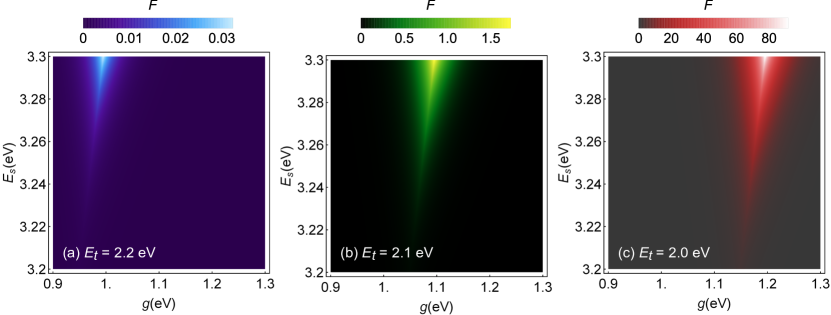
Fig. 2 shows as a function of and , with three different values of . It is important to notice the different scales in the different panels. It is also interesting to notice the slightly tilted maximum values of . Fig. 2 well illustrates the sensitivity of the problem; On one hand, even a slight increase of (or decrease of ) quickly kills . On the other, the range of of enhanced RISC is very narrow. In Fig. 2, we have used [15]
| (26) |
to evaluate . Here, is the refractive index of the medium, , is the length of the cavity, and is the in-plane momentum.
When bringing LP closer to the first-order triplet state, we inevitably enhance ISC as well. This is against our goal: to convert the slow triplets to fast singlets (or polaritons). However, one can notice from Eqs. (20) and (22) that while RISC is weighted by , ISC is weighted by . Therefore, if , we need to have in order for RISC to outdo ISC. This is an important point we want to highlight, since high RISC/ISC ratio can be achieved if the triplets have long enough lifetimes and the LP empties quickly enough by emission, losses, or dephasing. It is also worth mentioning that even though we have focused on LP, we might be able to harvest higher-order triplets with UP and “hot RISC” [28].
IV Toward higher dimensions
IV.1 Second-order polaritons
Being restricted to the single-excitation subspace, our model is unable to cover all the possible processes occurring in (polaritonic) OLEDs. By extending our model to encompass two-excitation polariton states, many crucial phenomena such as polariton-polariton interactions can start to unravel [35, 36, 37, 38, 39], providing a more comprehensive picture of polaritonic OLEDs. While the exploration of these processes is reserved for future research, here we lay out the stepping stones toward that.
Using the ansatz
| (27) |
where , and requiring it to satisfy , we arrive at the following system of equations,
| (28) |
Using the normalization condition of the second-order Hopfield coefficients and the approximation , we get
| (29) | ||||
| (30) | ||||
| (31) | ||||
| (32) | ||||
| (33) |
It might be tempting to write higher-order eigenvalues as similar mixtures of and and integer-multiples of . However, the higher the dimension of the system, the more erroneous the required approximation becomes, among other complications. Nevertheless, the form of already suggests that in higher dimensions the dilution of RISC might be much stronger, scaling polynomially with .
IV.2 Triplet-triplet annihilation
When two triplet excitons come within their capture radii, they form an encounter complex with the energy , which can then relax to two lower-energy states following the spin statistics, one of them being the ground state. This is known as triplet-triplet annihilation (TTA) [40]. In the context of this paper, TTA could be described by
| (34) | ||||
| (35) | ||||
| (36) | ||||
| (37) |
where is again the phase flip probability [cf. Eqs. (9) and (10)], , controlling interaction confinement near the capture radius ,
| (38) |
and ; If , their difference does not affect TTA [16]. Here, we would move from the two-excitation subspace to the single-excitation subspace.
Since polaritons are collective states and TTA an intermolecular process, one might anticipate more prominent enhancement with TTA than with the intramolecular RISC. However, the enhancement factor of TTA in our case (from the encounter complex to LP) becomes
| (39) |
which also dilutes with .
An interesting prospect arises if the triplets are sparsely created—i.e., outside their capture radii and therefore not promoting TTA—and if their transition dipole moment can no longer be neglected: Since the triplet polaritons would consist of all the possible permutations of triplet-occupied molecular sites, some of them might be within the capture radii and contribute to TTA.
IV.3 Singlet-singlet annihilation
When two singlet excitons interact, they are promoted to a higher-order excited singlet which then either relaxes back to the first-order singlets or ground state—releasing heat at the same time—or breaks into free charge carriers [41]. With thin and tightly packed recombination zones, as discussed earlier in the context of electrical excitation, this may lead to efficiency roll-off and device degradation [42]. This time it would be beneficial for strong coupling to separate such close singlets, opposite to what was just discussed with TTA.
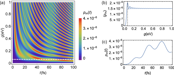
Single-excitation subspace is enough for us to clarify this idea. Consider the initial state , where the majority of are zero due to thin recombination zone. If the pump has been switched off and all the decay channels act on slowly enough, we can focus solely on the unitary dynamics induced by . The probability to find a singlet on site at time becomes which, after some algebra and defining , can be written as
| (40) |
In Fig. 3, we have plotted the singlet probability outside the recombination zone, i.e., when . Interestingly, when taking its average over multiple instances, an optimum value of can be observed from Fig. 3(b) ( meV). Here, the timespan was from 0 to 100 fs in timesteps of 0.1 fs. Fig. 3(c) shows at this optimum coupling strenght.
Fig. 3 essentially demonstrates that, even though electrical excitation may be spatially confined [see Eq. (11)], with strong coupling singlets can be formed beyond the recombination zone. OLEDs with polariton-improved operational lifetimes were recently reported in [6], to which our analysis ultimately provides an alternative (or complementary) explanation. In [6], however, the OLEDs were phosphorescent, but the same analysis holds for TTA.
V Conclusions
In this article, we investigated the incoherent dynamics of polariton OLEDs by employing a phenomenological master equation model within the linear regime. In addition, we outlined several nonlinear scenarios that strong coupling might influence. Our master equation model is comprehensive yet very simple—and hence it helps to better understand the rich open-system dynamics happening in polariton OLEDs. In the future, the model can be refined by taking into account all the interstate couplings and constructing the entire system-environment Hamiltonian. Here, the environment was treated only implicitly.
One of the main results of this paper is the enhancement factors of polaritonic RISC and TTA. Our approach predicts their dilution with the number of molecules, which is in line with previous works and was used as a benchmark. In the emerging field of polariton organic optoelectronics, the inverse-scaling problem is expected to hinder strong polariton-induced dynamics. Thus, comprehensive ruling out of Purcell enhancement [43] and polariton-induced spectral filtering with refocused emission intensity [44, 45] is necessary in future experiments.
Even though it might appear an elusive goal to fully harness triplets with polaritonic RISC and TTA, strong coupling might influence OLEDs in other, perhaps more surprising ways. Strong coupling can, in a sense, redistribute excitons. This can benefit fluorescent materials by either accelerating TTA or alternatively delaying SSA. While further research is needed to fully understand these fascinating new directions, strong coupling clearly holds tremendous potential for next-generation OLEDs.
Acknowledgments
This project has received funding from the European Research Council (ERC) under the European Union’s Horizon 2020 research and innovation programme (grant agreement No. [948260]). O.S. acknowledges the fruitful discussions with Arpan Dutta and Timo Leppälä.
References
- Forrest [2004] S. R. Forrest, The path to ubiquitous and low-cost organic electronic appliances on plastic, Nature 428, 911 (2004).
- Trindade et al. [2023] G. F. Trindade, S. Sul, J. Kim, R. Havelund, A. Eyres, S. Park, Y. Shin, H. J. Bae, Y. M. Sung, L. Matjacic, Y. Jung, J. Won, W. S. Jeon, H. Choi, H. S. Lee, J. C. Lee, J. H. Kim, and I. S. Gilmore, Direct identification of interfacial degradation in blue OLEDs using nanoscale chemical depth profiling, Nature Communications 14, 1 (2023).
- Tankelevičiūtė et al. [2024] E. Tankelevičiūtė, I. D. Samuel, and E. Zysman-Colman, The Blue Problem: OLED Stability and Degradation Mechanisms, Journal of Physical Chemistry Letters 15, 1034 (2024).
- Mischok et al. [2023] A. Mischok, S. Hillebrandt, S. Kwon, and M. C. Gather, Highly efficient polaritonic light-emitting diodes with angle-independent narrowband emission, Nature Photonics 17, 393 (2023).
- Yoshida et al. [2023] K. Yoshida, J. Gong, A. L. Kanibolotsky, P. J. Skabara, G. A. Turnbull, and I. D. W. Samuel, Electrically driven organic laser using integrated OLED pumping, Nature 621, 746 (2023).
- Zhao et al. [2024] H. Zhao, C. E. Arneson, D. Fan, and S. R. Forrest, Stable blue phosphorescent organic LEDs that use polariton-enhanced Purcell effects, Nature 626, 300 (2024).
- Uoyama et al. [2012] H. Uoyama, K. Goushi, K. Shizu, H. Nomura, and C. Adachi, Highly efficient organic light-emitting diodes from delayed fluorescence, Nature 492, 234 (2012).
- Sanvitto and Kéna-Cohen [2016] D. Sanvitto and S. Kéna-Cohen, The road towards polaritonic devices, Nature Materials 15, 1061 (2016).
- Feist et al. [2018] J. Feist, J. Galego, and F. J. Garcia-Vidal, Polaritonic Chemistry with Organic Molecules, ACS Photonics 5, 205 (2018).
- Hertzog et al. [2019] M. Hertzog, M. Wang, J. Mony, and K. Börjesson, Strong light-matter interactions: A new direction within chemistry, Chemical Society Reviews 48, 937 (2019).
- Stranius et al. [2018] K. Stranius, M. Hertzog, and K. Börjesson, Selective manipulation of electronically excited states through strong light–matter interactions, Nature Communications 9, 2273 (2018).
- Abdelmagid et al. [2024] A. G. Abdelmagid, H. A. Qureshi, M. A. Papachatzakis, O. Siltanen, M. Kumar, A. Ashokan, S. Salman, K. Luoma, and K. S. Daskalakis, Identifying the origin of delayed electroluminescence in a polariton organic light-emitting diode, Nanophotonics doi:10.1515/nanoph-2023-0587 (2024).
- Yu et al. [2021] Y. Yu, S. Mallick, M. Wang, and K. Börjesson, Barrier-free reverse-intersystem crossing in organic molecules by strong light-matter coupling, Nature Communications 12, 1 (2021).
- Eizner et al. [2019] E. Eizner, L. A. Martínez-Martínez, J. Yuen-Zhou, and S. Kéna-Cohen, Inverting singlet and triplet excited states using strong light-matter coupling, Science Advances 5, eaax4482 (2019).
- Bhuyan et al. [2023] R. Bhuyan, J. Mony, O. Kotov, G. W. Castellanos, J. Gómez Rivas, T. O. Shegai, and K. Börjesson, The rise and current status of polaritonic photochemistry and photophysics, Chemical Reviews 123, 10877 (2023).
- Ye et al. [2021] C. Ye, S. Mallick, M. Hertzog, M. Kowalewski, and K. Börjesson, Direct transition from triplet excitons to hybrid light–matter states via triplet–triplet annihilation, Journal of the American Chemical Society 143, 7501 (2021).
- Mukherjee et al. [2023] A. Mukherjee, J. Feist, and K. Börjesson, Quantitative Investigation of the Rate of Intersystem Crossing in the Strong Exciton–Photon Coupling Regime, Journal of the American Chemical Society 145, 5155 (2023).
- Martínez-Martínez et al. [2019] L. A. Martínez-Martínez, E. Eizner, S. Kéna-Cohen, and J. Yuen-Zhou, Triplet harvesting in the polaritonic regime: A variational polaron approach, Journal of Chemical Physics 151, 054106 (2019).
- Rebentrost et al. [2009] P. Rebentrost, M. Mohseni, and A. Aspuru-Guzik, Role of quantum coherence and environmental fluctuations in chromophoric energy transport, The Journal of Physical Chemistry B 113, 9942 (2009).
- Nakano et al. [2016] M. Nakano, S. Ito, T. Nagami, Y. Kitagawa, and T. Kubo, Quantum master equation approach to singlet fission dynamics of realistic/artificial pentacene dimer models: Relative relaxation factor analysis, The Journal of Physical Chemistry C 120, 22803 (2016).
- Herrera and Spano [2017] F. Herrera and F. C. Spano, Absorption and photoluminescence in organic cavity qed, Physical Review A 95, 053867 (2017).
- Takahashi et al. [2019] S. Takahashi, K. Watanabe, and Y. Matsumoto, Singlet fission of amorphous rubrene modulated by polariton formation, The Journal of Chemical Physics 151, 074703 (2019).
- Gu and Mukamel [2021] B. Gu and S. Mukamel, Optical-cavity manipulation of conical intersections and singlet fission in pentacene dimers, The Journal of Physical Chemistry Letters 12, 2052 (2021).
- Carreras and Casanova [2022] A. Carreras and D. Casanova, Theory of exciton dynamics in thermally activated delayed fluorescence, ChemPhotoChem 6, e202200066 (2022).
- Ćwik [2015] J. A. Ćwik, Organic polaritons : modelling the effect of vibrational dressing, Ph.D. thesis, University of St Andrews (2015).
- Hopfield [1958] J. J. Hopfield, Theory of the contribution of excitons to the complex dielectric constant of crystals, Physical Review 112, 1555 (1958).
- Breuer and Petruccione [2007] H.-P. Breuer and F. Petruccione, The Theory of Open Quantum Systems (Oxford University Press, 2007).
- Lin et al. [2021] C. Lin, P. Han, S. Xiao, F. Qu, J. Yao, X. Qiao, D. Yang, Y. Dai, Q. Sun, D. Hu, A. Qin, Y. Ma, B. Z. Tang, and D. Ma, Efficiency Breakthrough of Fluorescence OLEDs by the Strategic Management of “Hot Excitons” at Highly Lying Excitation Triplet Energy Levels, Advanced Functional Materials 31, 1 (2021).
- Cheon and Shinar [2004] K. O. Cheon and J. Shinar, Electroluminescence spikes, turn-off dynamics, and charge traps in organic light-emitting devices, Physical Review B 69, 201306 (2004).
- Duan et al. [2011] L. Duan, D. Zhang, K. Wu, X. Huang, L. Wang, and Y. Qiu, Controlling the recombination zone of white organic light-emitting diodes with extremely long lifetimes, Advanced Functional Materials 21, 3540 (2011).
- Gerry and Knight [2005] C. Gerry and P. Knight, Introductory Quantum Optics (Cambridge University Press, 2005).
- Palo and Daskalakis [2023] E. Palo and K. S. Daskalakis, Prospects in Broadening the Application of Planar Solution‐Based Distributed Bragg Reflectors, Advanced Materials Interfaces 10, 2202206 (2023).
- Marian [2012] C. M. Marian, Spin–orbit coupling and intersystem crossing in molecules, WIREs Computational Molecular Science 2, 187 (2012).
- Ou et al. [2021] Q. Ou, Y. Shao, and Z. Shuai, Enhanced reverse intersystem crossing promoted by triplet exciton–photon coupling, Journal of the American Chemical Society 143, 17786 (2021).
- Daskalakis et al. [2014] K. S. Daskalakis, S. A. Maier, R. Murray, and S. Kéna-Cohen, Nonlinear interactions in an organic polariton condensate, Nature Materials 13, 271 (2014).
- Plumhof et al. [2014] J. D. Plumhof, T. Stöferle, L. Mai, U. Scherf, and R. F. Mahrt, Room-temperature Bose–Einstein condensation of cavity exciton–polaritons in a polymer, Nature Materials 13, 247 (2014).
- Ramezani et al. [2017] M. Ramezani, A. Halpin, A. I. Fernández-Domínguez, J. Feist, S. R.-K. Rodriguez, F. J. Garcia-Vidal, and J. Gómez Rivas, Plasmon-exciton-polariton lasing, Optica 4, 31 (2017).
- Väkeväinen et al. [2020] A. I. Väkeväinen, A. J. Moilanen, M. Nečada, T. K. Hakala, K. S. Daskalakis, and P. Törmä, Sub-picosecond thermalization dynamics in condensation of strongly coupled lattice plasmons, Nature Communications 11, 3139 (2020).
- Zasedatelev et al. [2021] A. V. Zasedatelev, A. V. Baranikov, D. Sannikov, D. Urbonas, F. Scafirimuto, V. Y. Shishkov, E. S. Andrianov, Y. E. Lozovik, U. Scherf, T. Stöferle, R. F. Mahrt, and P. G. Lagoudakis, Single-photon nonlinearity at room temperature, Nature 597, 493 (2021).
- Wallikewitz et al. [2012] B. H. Wallikewitz, D. Kabra, S. Gélinas, and R. H. Friend, Triplet dynamics in fluorescent polymer light-emitting diodes, Physical Review B 85, 045209 (2012).
- King et al. [2007] S. M. King, D. Dai, C. Rothe, and A. P. Monkman, Exciton annihilation in a polyfluorene: Low threshold for singlet-singlet annihilation and the absence of singlet-triplet annihilation, Physical Review B 76, 085204 (2007).
- Gather et al. [2011] M. C. Gather, A. Köhnen, and K. Meerholz, White Organic Light-Emitting Diodes, Advanced Materials 23, 233 (2011).
- Vahala [2003] K. Vahala, Optical microcavities, Nature 424, 839 (2003).
- Daskalakis et al. [2019] K. S. Daskalakis, F. Freire-Fernández, A. J. Moilanen, S. van Dijken, and P. Törmä, Converting an Organic Light-Emitting Diode from Blue to White with Bragg Modes, ACS Photonics 6, 2655 (2019).
- Khazanov et al. [2023] T. Khazanov, S. Gunasekaran, A. George, R. Lomlu, S. Mukherjee, and A. J. Musser, Embrace the darkness: An experimental perspective on organic exciton-polaritons, Chemical Physics Reviews 4, 041305 (2023).