Zeno physics of the Ising chain with symmetry-breaking boundary dephasing

Abstract

In few-qubit systems, the quantum Zeno effect arises when measurement occurs sufficiently frequently that the spins are unable to relax between measurements. This can compete with Hamiltonian terms, resulting in interesting relaxation processes which depend non-monotonically on the ratio of measurement rate to coherent oscillations. While Zeno physics for a single qubit is well-understood, an interesting open question is how the Zeno effect is modified by coupling the measured spin to a non-trivial bulk. In this work, we study the effect of coupling a one-dimensional transverse field Ising to a Zeno spin which lives at the boundary. We find that sharp singularities occur in the boundary relaxation dynamics, which can be tied to the emergence or destruction of edge modes that can be found analytically. Finally, we provide numerical evidence that the dynamical singularities are stable in the presence of integrability-breaking interactions.

Figure 1: Illustration of Ising model with symmetry-breaking boundary noise. Far from the boundary, the Ising model is in its ground state ($T=0$). Boundary spin dynamics show singularities which can be connected to edge modes, resulting in a nontrivial boundary phase diagram.

Understanding the nature of non-equilibrium correlated phases of matter in many-body systems beyond the perturbative regime is challenging. Yet nonequilibrium quantum physics is precisely the regime that is increasingly experimentally accessible in systems ranging from cold atoms and ions to superconducting circuits to (noisy) quantum computers [1, 2, 3]. Therefore, characterizing nonequilibrium quantum systems and their phases of matter is one of the most important questions in many-body physics today.

Given the dearth of solvable non-equilibrium models, it is crucial to develop an in-depth understanding of the few models in which analytical methods exist. One important class of such systems are quantum boundary/impurity models. Examples where these can be treated beyond the perturbative limit include the Anderson impurity [4, 5, 6, 7, 8, 9], transport in one-dimensional junctions with strong electron-electron interactions  [10, 11], and the generation and growth of entanglement among magnetic impurities and their surrounding environments in the Kondo effect  [12, 13, 14]. A key tool for addressing many of these example systems is boundary conformal field theory (CFT), which uses generalized scale invariance near quantum critical points to build a significant analytical toolkit [15, 16, 17, 18, 19, 20, 21].

However, most results in boundary CFT do not address the increasingly important situation of open quantum systems. Motivated by developments in quantum simulation and computation, it is increasingly important to consider quantum systems which are driven far-from-equilibrium yet, inevitably, remain coupled to their environments. Despite hindering some goals of quantum information theory, dissipation has been found to be useful in other ways such as aiding in state preparation [22, 23, 24] and enhancing the phase structure of quantum matter [25, 26, 27]. Nonequilibrium open quantum systems are even harder to treat in the strongly correlated regime, necessitating the study of models where concrete predictions can be made.

In this paper, we show that the transverse field Ising chain with symmetry-breaking boundary dephasing enables analytical predictions for the boundary dynamics. Despite symmetry breaking at the boundary, it remains integrable, with certain correlation functions expressible in the language of free Majorana fermions. Edge modes emerge which are naturally described in terms of the Majoranas, giving rise to an interesting (boundary) phase diagram. Furthermore, we show that these edge modes are directly connected to boundary spin dynamics, such that the appearance or disappearance of edge modes coincides with sharp changes in the dynamics. We argue that these singularities are robust to integrability-breaking interactions in the appropriate scaling limit and support the argument with matrix product state-based numerics. Finally, we argue that this is a fundamentally nonequilibrium phenomenon that is hidden from conventional equilibrium observables. We show this explicitly for the steady state energy current from the bath and boundary magnetic susceptibility.

I Model

We consider the one-dimensional Ising model with open boundary conditions and dephasing that breaks Ising symmetry at the boundary. Specifically, we assume non-unitary time evolution of the Lindblad form,

$$\frac{d\rho}{dt}=\mathcal{L}[\rho]=-i[H,\rho]+L\rho L^{\dagger}-\frac{1}{2}\{L^{\dagger}L,\rho\},$$ (1)

with Hamiltonian

$$H=-J\sum_{n=1}^{L-1}\sigma_{n}^{z}\sigma_{n+1}^{z}-h\sum_{n=1}^{L}\sigma_{n}^{x}$$ (2)

and a single Lindblad operator

$$L=\sqrt{\gamma}\sigma_{1}^{z}.$$ (3)

We use the convention $J=\hbar=1$ throughout.

We are interested in the dynamics of the boundary spin, $\sigma^{z}_{1}$, in the presence of this boundary dephasing. One motivation for this is the quantum Zeno effect, which for $J=0$ (single spin) says that the spin dynamics get frozen in the limit $\gamma\gg h$ due to repeated measurements by the environment. By adding interactions $J>0$, we wish to understand the effect of many-body physics – including quantum phase transitions – on Zeno physics. Furthermore, the phase transition in the Ising model is a canonical example of a conformal field theory (CFT). By coupling this system to a noisy, relevant boundary perturbation, there is hope to draw a connection between many-body Zeno physics and boundary CFT. Similar ideas have been explored in recent works [28, 29, 30], but addressing much different questions. Specifically, [28] considered a random boundary drive but only in a strongly driven limit that falls outside of the Lindblad approximation and studied many-body Loschmidt echo. [29] and [30] studied dissipative impurity models similar to ours, but focused on alternative observables such as transport and non-Gaussian correlations that have direct connection to two-time correlations, which is the more conventional observable used to define Zeno physics. By contrast, we study two-time correlations of a boundary impurity, where we will analytically solve for modifications of the (boundary) Zeno effect.

In the absence of static symmetry-breaking boundary field, the spin itself is unpolarized. Therefore, the quantity of interest is the two-time correlation function, which is related to the boundary magnetic susceptibility. Specifically, we seek to find the two-time correlation function in the time-evolved density matrix $\rho(t)$, which is given by using the regression theorem [31]:

$$C(t,\Delta t)=\langle\sigma_{1}^{z}(t+\Delta t)\sigma_{1}^{z}(t)\rangle=\mathrm{Tr}\left\{\left[e^{\mathcal{L^{\dagger}}\Delta t}\sigma_{1}^{z}\right]\sigma_{1}^{z}\rho(t)\right\},$$ (4)

where the adjoint Liouvillian $\mathcal{L}^{\dagger}$ generates Heisenberg operator evolution. The initial state is $\rho(0)=|\psi_{\mathrm{gs}}\rangle\langle\psi_{\mathrm{gs}}|$, the ground state of the unperturbed Ising chain ($\gamma=0$). Then, at $t=0$, a finite value of $\gamma$ is quenched on. Once we introduce this noise at the edge, we expect quasiparticle excitations to travel ballistically to the other edge of the chain in time $t\approx L/v$. Outside the ballistic front ($x>vt$), the system remains in its ground state. Inside the ballistic front ($x<vt$), the system approaches a new quasi-stationary state in which excitations are continuously added via the boundary dephasing. We are interested in this quasi-stationary non-equilibrium steady state (NESS) that forms near the boundary for $t+\Delta t<L/v$. In order to equilibrate to the local NESS, $t$ must be chosen to be sufficiently large as well; we use $t=40$ throughout our data. Note that this should be equivalent to the true NESS that forms for a large, zero temperature bath placed sufficiently far from the perturbed boundary (see Figure 1).

Numerically calculating the two-time autocorrelation function remains challenging in general, but for this particular model it can be efficiently obtained by rewriting in terms of Majorana fermions. We start by a conventional Jordan-Wigner transform on the spin degrees of freedom [32],

$$\sigma_{j}^{x}=i\eta_{2j-1}\eta_{2j},\ \sigma_{j}^{z}=\left(\prod_{n=1}^{j-1}i\eta_{2n-1}\eta_{2n}\right)\eta_{2j-1}.$$ (5)

The boundary spin is then a single Majorana operator, $\sigma_{1}^{z}=\eta_{1}$, and the Hamiltonian can be written as

$$H=-ih\sum_{j=1}^{L}\eta_{2j-1}\eta_{2j}-iJ\sum_{j=1}^{L-1}\eta_{2j}\eta_{2j+1}.$$ (6)

The first step is to evolve the density matrix to $\rho(t)$ and calculate the equal-time correlation function $C(t,0)=\mathrm{Tr}\left[\sigma_{1}^{z}\sigma_{1}^{z}\rho(t)\right]=\mathrm{Tr}\left[\eta_{1}^{2}\rho(t)\right]$. Since $\eta_{1}^{2}=1$, this is always equal to $1$. Crucially, we can also calculate the full Majorana correlation matrix $\mathcal{C}_{ij}(t,0)=\mathrm{Tr}\left[\eta_{i}\eta_{j}\rho(t)\right]$ such that $C=\mathcal{C}_{11}$. Two-time correlation functions are then able to be calculated because the adjoint Liouvillian conserves Majorana number:

$$\mathcal{L}^{\dagger}\left[\eta_{i}\right]=i[H,\eta_{i}]+\gamma(\eta_{1}\eta_{i}\eta_{1}-\eta_{i})=\sum_{j=1}^{2L}M_{ij}\eta_{j}.$$ (7)

The matrix $M$ has the form

$$M=\left(\begin{array}[]{cccc}0&-2h&0&0\\ 2h&-2\gamma&-2J&0\\ 0&2J&-2\gamma&-2h\\ 0&0&2h&\ddots\end{array}\right).$$ (8)

One can then readily show that the 2-time correlation matrix evolves as

$$\frac{\partial\mathcal{C}(t,\Delta t)}{\partial\Delta t}=M\mathcal{C}(t,\Delta t)$$ (9)

with equal-time correlations, $\mathcal{C}(t,0)$, as an initial condition. Clearly the eigenmodes of $M$ play a crucial role in understanding the dynamics of the boundary spin; we therefore refer to this as the single-Majorana evolution matrix. More details for how these equations are solved numerically may be found in the supplement VII.1.

We note briefly that an alternative route to solving the open quantum dynamics exists by vectorizing the density matrix and treating the Lindblad evolution via third quantization. This doubles the effective Hilbert space, but manifestly makes the problem integrable because the boundary dephasing maps to a non-Hermitian Ising term connecting the bra and ket Hilbert spaces. A similar technique was used in recent papers [33, 34], which studied the related problem of dephasing connected to both ends of a finite system and found a similar phase diagram of the edge modes. While formally identical to our method, third quantization makes it more challenging to connect spectral features and eigenmodes of the Liouvillian to physical observables, so we primarily use the single-particle evolution matrix throughout this paper. More details on the third quantization formalism and its connection to the single-particle evolution matrix $M$ can be found in the supplementary information in sections VIII.1 and VIII.2.

II Results

Using the free fermionic form, we numerically solve for the 2-time correlations of the boundary spin. For all parameters chosen, the (complex-valued) autocorrelation function is found to decay exponentially at late times $\Delta t$ as $C\sim C_{0}\exp[-\Delta t/\tau]$, where $\tau$ is the relaxation time scale the characterizes the Zeno effect. At short times $\Delta t$, other fast-decaying eigenmodes of $M$ participate in the dynamics, spoiling the simple exponential decay. We fit the numerical data for large $\Delta t$ to extract a value of $\tau$, as shown in Figure 2 a.

Plotting the relaxation rate $\tau^{-1}$ as a function of $\gamma$ and $h$ (Figure 2b), we find the striking result that, for $h\geq 1$, sharp singularities occur in this decay constant in a fashion reminiscent of equilibrium observables in a conventional first order phase transition. These singularities separate the parameter space into three distinct phases (Figure 1, bottom), which we label paramagnet (PM), ferromagnet (FM)/Zeno, and anti-Zeno. The PM and FM smoothly connect to the respective ground state phases at $\gamma=0$ with a transition that extends vertically from $h=J$. The anti-Zeno phase only appears at $\gamma>J$ and, as we will see, cannot be thought of as smoothly connected to the ground state Ising physics.

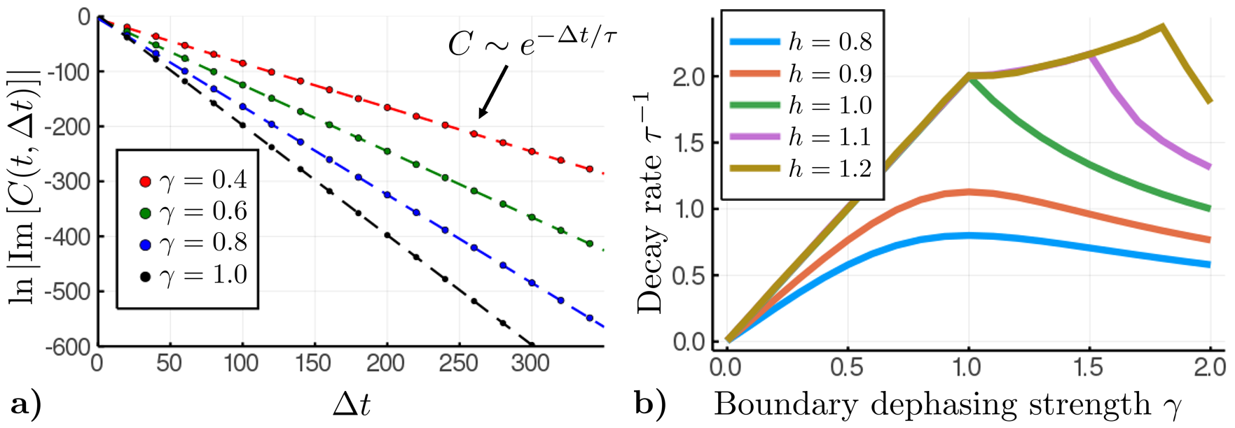
Figure 2: (a) Numerical results for two-time correlation function of the edge spin as a function of boundary dephasing rate ($\gamma$) for $L=1000$, $J=h=1$, and $t=40$. (b) Plot of decay rate $\tau^{-1}$ as a function of $\gamma$ for different values of $h$.

In order to understand the origin of these singularities, an interesting analogy can be drawn to our previous work [35], which examined the Ising chain with a static symmetry-breaking boundary field. There, we observed a connection between the two-time correlation function of the edge spin and emergent edge modes in the Majorana problem. While this setup is qualitatively different, we are inspired to ask a similar question of the effective non-Hermitian matrix $M$ which determines time evolution of the Majorana correlations. We begin by solving the eigenmodes of $M$ numerically, results of which are shown in Figure 3b. There are clearly modes that appear outside of the bulk, which we confirm are edge modes localized near the site with dephasing. Furthermore, we confirm that the change in edge mode counting is directly tied to the singularities in $\tau$.

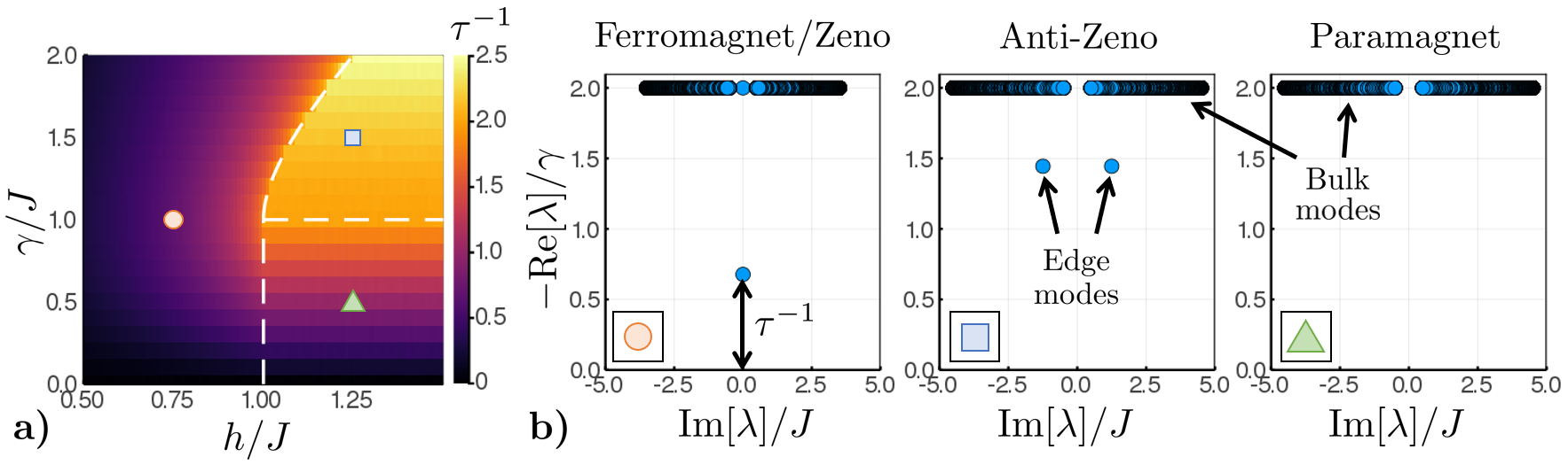
Figure 3: (a) Phase diagram obtained from singularities of the relaxation rate $\tau^{-1}$. (b) Eigenvalues $\lambda$ of the Majorana evolution matrix $M$ plotted for three different points in the phase diagram (left panel), showing number and structure of edge modes. The decay rate is set by the mode with the smallest magnitude real component.

In fact, we can go one step further and solve for the edge modes of $M$ as well as their phase transitions analytically. We consider the following (unnormalized) ansatz for the edge mode

$$\eta_{\text{edge}}=\sum_{j=1}^{N}\left(r^{j-1}\eta_{2j-1}+Ar^{j-1}\eta_{2j}\right),$$ (10)

where $\Big{|}r=e^{-1/\xi+i\varphi}\Big{|}<1$ describes the decay with length scale $\xi>0$. We are interested in the “eigenenergy” $\lambda$ such that $M\eta_{\mathrm{edge}}=\lambda\eta_{\mathrm{edge}}$. This equation is solved in the section VII.2, from which we observe that the number of physically meaningful edge modes ($|r|<1$) changes sharply at phase boundaries given by

$$h_{c}=\begin{cases}J&\mathrm{for}~{}\gamma<J\\ \frac{\gamma^{2}+J^{2}}{2\gamma}&\mathrm{for}~{}\gamma>J\end{cases}$$ (11)

Moreover, this analytical solution provides a complete description of the edge modes and their phase transitions, allowing us to re-interpret the observed dynamical signatures physically. For example, we readily see that the PM and FM edge modes track continuously to the Majorana zero modes of the Kitaev chain as $\gamma\to 0$. As $h$ approaches $J$ from the FM side, the edge mode gap approaches the bulk dephasing rate of $2\gamma$, such that the edge mode merges into the bulk simultaneously with the bulk gap closing at $h=J$. The phase transition looks similar to the conventional ground state Ising transition, with diverging edge correlation length $\xi\to\infty$ and a dissipative gap $\Delta\sim|h-J|$ suggesting that $\nu=z=1$ as in the ground state.

Another relatively simple limit of the model is $\gamma\gg J$, for which the physics of the single boundary spin becomes dominant. In this case, the limits $\gamma\ll h$ and $\gamma\gg h$ correspond to the anti-Zeno and Zeno regimes, respectively. While there is not a conventional phase transition in the steady state of the single-spin Zeno model, there is an exceptional point (i.e. under- to over-damped) transition at $\gamma_{c}=2h$. This is precisely the asymptote that we find for our phase boundary when $\gamma,h\gg J$. However, all the way down to $\gamma=J$ there is an exceptional point transition in the spectrum of $M$, allowing us to argue that one has Zeno and anti-Zeno “phases.”

The final boundary transition happens at $\gamma=J$ for $h>J$, between the PM and anti-Zeno phases. At this transition, two non-Hermitian bound states emerge out of the PM continuum at finite momentum. The critical behavior appears Ising-like, with imaginary gap that opens linearly with the tuning parameter $\gamma$ ($\nu=z=1$). Furthermore, the entire transition line has diverging correlation length $\xi\to\infty$ (i.e., $|r|\to 1$) but non-zero momentum $\varphi\neq 0$ except at the tricritical point $h=J=\gamma$. While this transition occurs at finite dephasing strength and away from bulk criticality, this diverging length scale suggests that an appropriately defined field theory with gapped bulk may be possible to construct, for which the transition may be universal.

III Integrability breaking perturbations

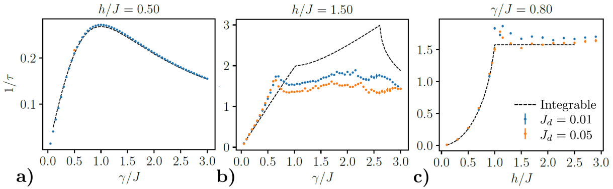
Figure 4: Relaxation rate extracted from TEBD simulations of the Ising chain with self-dual interactions for three cuts through the phase diagram: (a) $h/J=0.5$, for which no phase boundary is expected, (b) $h/J=1.5$, for which we expect to go from PM to anti-Zeno and finally to FM/Zeno, and (c) $\gamma/J=0.8$, which should cross the PM/FM phase boundary. The results are given by fitting either a pure exponential $e^{-\Delta t/\tau}$ or one dressed by a power law $(\Delta t)^{-3/2}e^{-\Delta t/\tau}$ in the $h>1$ and $\gamma<1$ region. The dashed lines in the plots $1/\tau$ are the results from the integrable case. For small $\gamma$, oscillations are still clearly present in $C(t,\Delta t)$ for the small $\Delta t$ available, making the fitting procedures less accurate.

In order to probe universality of this phase diagram, we now study the robustness of this edge physics in the presence of integrability-breaking interactions. We will do so by modifying the Hamiltonian to

$$\begin{split}H_{\mathrm{int}}=&-J\sum_{j}\sigma^{z}_{j}\sigma^{z}_{j+1}-h\sum_{j}\sigma^{x}_{j}+\\ &-J_{d}\sum_{j}\left(\sigma^{x}_{j}\sigma^{x}_{j+1}+\sigma^{z}_{j}\sigma^{z}_{j+2}\right).\end{split}$$ (12)

The form of the interaction is chosen such that it is invariant under the Kramers-Wannier (spin/bond) duality, meaning that if a ground state phase transition exists in the bulk, it must occur at the self-dual point $h=J$.

Since free fermion methods do not work for this interacting model, we must resort to alternative numerical methods. Specifically, we solve the dynamics via a variant of time-evolving block decimation (TEBD) in which the density matrix is treated in third quantization and unfolded such that boundary dephasing becomes a non-Hermitian perturbation at the center of the spin chain (see supplement VIII.1). We measure the autocorrelation functions for various $J_{d}>0$ (a ferromagnetic perturbation) after first evolving to time $t=1/J$. We consider system size $L=30$, which is sufficient to approximate $L=\infty$ for the timescales we are able to simulate, since no appreciable finite-size effects occur before $t\sim L/J$ .

We tested our methods by first applying them to the integrable case $J_{d}=0$ (see X.1) to confirm that it reproduced the known analytical and numerical results from free fermions. One issue that arises in the TEBD numerics is the relatively small $\Delta t\sim 15$ that can be accessed numerically. Specifically, within the PM phase a simple exponential does not fit the data well. The origin of this mismatch comes from the absence of edge modes, meaning that relaxation in the PM comes from the bulk continuum. However, after extracting the exponential prefactor, the remaining power law decay of the boundary spin correlations is strikingly similar to that of the Ising chain with static boundary field [35]. Calculating this decay via saddle point approximation gives a $t^{-3/2}$ multiplying the exponential, which is found to give a much cleaner fit and therefore reproduce $\tau^{-1}$ more accurately.

We then apply the same fitting procedure to the values of $C(t,\Delta t)$ obtained in the presence of integrability-breaking interactions. The results (in Figure 4) are far from clear, but do show strong signatures of the same phase transitions at both the PM/anti-Zeno and FM/PM transitions. This suggests that the transitions do indeed survive on this time scale despite the presence of integrability breaking. Furthermore, while the data does not resolve a singularity between the FM/Zeno and anti-Zeno phase due to the accessible short times, that limit is expected to be the most robust to interactions because it occurs on finite length scale $\xi$, which becomes particularly small in the limit $h,\gamma\gg J$. We therefore speculate that all the transitions survive interactions on this time scale, though detecting them may be challenging.

At late time $t+\Delta t\gg L/v$, one expects the system to heat up. With just boundary dephasing, the eventual steady state would correspond to infinite temperature. However, there are a few caveats which open the possibility that some of these phenomena will be infinitely long-lived. First, if the chain is semi-infinite, then time $L/v$ can never be reached. This is quite similar to the situation shown in Figure 1 in the sense that the semi-infinite chain can be thought of as an unbounded zero temperature heat sink. If the mean free path $\ell_{\mathrm{mfp}}$ is much longer than the edge mode localization length $\xi$, then one would expect these excitations to be carried out of the system by the zero temperature bath before they can backscatter and thermalize the edge mode. The precision of this statement, including whether it turns transitions into crossovers, remains unclear; it will be an important topic for future investigation.

IV Single-time observables

Having identified the emergence of edge modes that are tied to the dynamical singularities, we may expect that signatures of these edge modes will also show up in other observables signifying properties of the nonequilibrium steady state. In the supplementary material, we study magnetic susceptibility and energy current in the NESS (sections IX.2 and IX.1). We find no evidence for singularities of either quantity. This is tied to the evolution of the equal-time correlation matrix $\mathcal{C}(t,\Delta t=0)$, which is governed by a matrix similar to $M$ but with exponential decay of the edge rather than bulk. This reduces the impact of the edge modes in quasi-equilibrium observables and, as we argue in the supplement, appears to prevent singularities in these quantities. Therefore, we conclude that the edge transitions are a dynamical phenomenon which are not captured by conventional equilibrium properties.

V Conclusion

We have investigated the transverse field Ising chain in the presence of boundary dephasing. We calculated the decay rate of two-time correlations of the boundary spin and showed that sharp singularities occur in between the Zeno and anti-Zeno regimes. The corresponding phase diagram divides into three distinct phases whose boundary relaxation dynamics are directly tied to analytically solvable edge modes in the related Majorana problem. This phase diagram appears robust to interactions in TEBD simulations, consistent with our prediction that the dynamical phenomena will be universal within one-dimensional models with Ising symmetry.

Our results have potentially far-reaching implications if they can be generalized to open versions of other well-studied models, most notably boundary CFTs with dephasing that couples to a relevant boundary perturbations with larger critical exponents. For the Ising CFT with symmetry-breaking boundary magnetic field, the perturbation is relevant near the static Hamiltonian ground state. However, if one attempts to apply similar renormalization group analysis to the symmetry-breaking boundary Lindbladian using Keldysh field theory, one finds that the Lindblad dephasing is marginal. Since the FM/PM transition remains unmodified by weak $\gamma$, we argue that $\gamma$ is marginally irrelevant. By contrast, for the Potts models with $\mathds{Z}_{q}$ symmetry, a similar Keldysh renormalization group analysis suggests that symmetry-breaking boundary dephasing is relevant for $q\geq 3$ [36]. This would imply the creation of a new boundary phase near the critical point; our work to find this behavior remains on-going. Similar non-unitary boundary terms can be studied for a wide class of models, including experimentally relevant situations such as a dissipative Kondo problem which is known to be equivalent to a boundary CFT [37]. Finally, we note that dissipative impurity problems are naturally created in a variety of experimental settings where their dynamics remain challenging to solve. One important example of this is resonant inelastic x-ray scattering (RIXS), in which a localized “core hole” impurity modifies the dynamics of the itinerant electrons around it. The problem naturally involves relaxation dynamics as electrons attempt to fill this hole. Therefore, we hope that some of the techniques that we have developed here for an analytically tractable Ising model with boundary dephasing can be generalized to this more challenging, but experimentally relevant, setting.

VI Acknowledgments

We greatly thank Matthew Foster and Romain Vasseur for helpful discussions. This work was performed with support from the National Science Foundation (NSF) through award numbers MPS-2228725 and DMR-1945529, the Welch foundation through award number AT-2036-202004, and the University of Texas at Dallas Office of Research (M.K. and U.J.). Part of this work was performed at the Aspen Center for Physics, which is supported by NSF grant No. PHY-1607611. The work of RJVT and JM has been supported by the Deutsche Forschungsgemeinschaft (DFG, German Research Foundation) through the grant HADEQUAM-MA7003/3-1; by the Dynamics and Topology Center, funded by the State of Rhineland Palatinate. Parts of this research were conducted using the Mogon supercomputer and/or advisory services offered by Johannes Gutenberg University Mainz (hpc.uni-mainz.de), which is a member of the AHRP (Alliance for High Performance Computing in Rhineland Palatinate, www.ahrp.info), and the Gauss Alliance e.V. RJVT and JM gratefully acknowledge the computing time granted on the Mogon supercomputer at Johannes Gutenberg University Mainz (hpc.uni-mainz.de) through the project “DysQCorr.” The Flatiron Institute is a division of the Simons Foundation.

Supplementary information

In this supplement, we provide additional information and data on Majorana time evolution, analytical solutions for the edge states, third-quantized treatments of the dynamics, equilibrium observables, and computational methods for the integrability-breaking model.

VII Details regarding second-quantized Majorana time evolution

Throughout the main text, we primarily solve Majorana correlation functions using their direct Heisenberg time evolution. In this section, we provide more details on how this is done numerically. We also solve for the edge states analytically in a semi-infinite geometry.

VII.1 Numerics for 1- and 2-time correlation functions

The time evolution of our system is given by the Lindblad equation

$$\frac{d\rho}{dt}=\mathcal{L}[\rho]=-i[H,\rho]+L\rho L^{\dagger}-\frac{1}{2}\{L^{\dagger}L,\rho\}$$ (13)

where $\mathcal{L}$ is the Liouvillian super-operator and $L$ is a Lindblad operator which has the form

$$L=\sqrt{\gamma}\sigma_{1}^{z}$$ (14)

Using the Jordan-Wigner transformation, we can write our Hamiltonian and Lindblad operator in terms of Majorana fermions as:

$$H =-iJ\sum_{n=1}^{L-1}\eta_{2n}\eta_{2n+1}-ih\sum_{n=1}^{L}\eta_{2n-1}\eta_{2n}\equiv i\eta^{T}A\eta$$ (15)

$$L =\sqrt{\gamma}\eta_{1}$$ (16)

where

$$A=\begin{pmatrix}0&-h/2\\ h/2&-0&-J/2\\ &J/2&0&-h/2\\ &&h/2&0\\ &&&&\ddots\end{pmatrix}$$ (17)

is an $2L\times 2L$ real antisymmetric matrix and $\eta=(\eta_{1},\eta_{2},\eta_{3},\ldots)^{T}$ is a column vector of Majorana operators.

We are interested in calculating a 2-time correlation function of the Majoranas starting from initial state $\rho(t=0)$, which is given by the regression theorem [31] as

$$\mathcal{C}_{ij}(t,\Delta t)=\mathrm{Tr}\left[\eta_{i}e^{\mathcal{L}\Delta t}\left(\eta_{j}\rho(t)\right)\right]$$ (18)

First, let’s calculate the time evolution of the equal-time correlation function, $\Delta t=0$. Note that the diagonal elements are always equal to

$$\mathcal{C}_{jj}\left(t,0\right)=\mathrm{Tr}\left[\eta_{j}^{2}\rho(t)\right]=1.$$ (19)

The time derivative of the off-diagonal terms ($i\neq j$) is

$$\frac{d\mathcal{C}_{ij}}{dt} =\text{Tr}\left[\eta_{i}\eta_{j}\frac{d\rho}{dt}\right]$$ (20)

$$=\text{Tr}\left[\eta_{i}\eta_{j}\left(-i[H,\rho]+L\rho L^{\dagger}-\rho\right)\right]$$ (21)

$$=\text{Tr}\left[\eta_{i}\eta_{j}\left(\sum_{kl}A_{kl}[\eta_{k}\eta_{l},\rho]+\gamma\eta_{1}\rho\eta_{1}-\gamma\rho\right)\right]$$ (22)

Despite appearing to involve 4-point correlation functions of the Majoranas, we can simplify the above equation to only involve 2-point correlations by using the anticommutation relations for our Majorana operators, $\{\eta_{i},\eta_{j}\}=2\delta_{ij}$, as well as cyclicity of the trace and antisymmetry of $A$ and $\mathcal{C}$:

$$\sum_{kl}A_{kl}\text{Tr}\left(\eta_{i}\eta_{j}[\eta_{k}\eta_{l},\rho]\right) =\sum_{kl}A_{kl}\text{Tr}\left(\left[\eta_{i}\eta_{j},\eta_{k}\eta_{l}\right]\rho\right)$$ (23)

$$=\sum_{kl}A_{kl}\left\langle\eta_{i}\eta_{j}\eta_{k}\eta_{l}-\eta_{k}\eta_{l}\eta_{i}\eta_{j}\right\rangle$$ (24)

$$=\sum_{kl}A_{kl}\left\langle\eta_{i}\eta_{j}\eta_{k}\eta_{l}-2\delta_{il}\eta_{k}\eta_{j}+\eta_{k}\eta_{i}\eta_{l}\eta_{j}\right\rangle$$ (25)

$$=\sum_{kl}A_{kl}\left\langle\eta_{i}\eta_{j}\eta_{k}\eta_{l}-2\delta_{il}\eta_{k}\eta_{j}+2\delta_{ik}\eta_{l}\eta_{j}-\eta_{i}\eta_{k}\eta_{l}\eta_{j}\right\rangle$$ (26)

$$=\sum_{kl}A_{kl}\left\langle\eta_{i}\eta_{j}\eta_{k}\eta_{l}-2\delta_{il}\eta_{k}\eta_{j}+2\delta_{ik}\eta_{l}\eta_{j}-2\delta_{jl}\eta_{i}\eta_{k}+\eta_{i}\eta_{k}\eta_{j}\eta_{l}\right\rangle$$ (27)

$$=\sum_{kl}A_{kl}\left\langle-2\delta_{il}\eta_{k}\eta_{j}+2\delta_{ik}\eta_{l}\eta_{j}-2\delta_{jl}\eta_{i}\eta_{k}+2\delta_{jk}\eta_{i}\eta_{l}\right\rangle$$ (28)

$$=2\sum_{kl}\left[\delta_{il}\mathcal{C}_{jk}A_{kl}+\delta_{ik}A_{kl}\mathcal{C}_{lj}-\delta_{jl}\mathcal{C}_{ik}A_{kl}-\delta_{jk}A_{kl}\mathcal{C}_{li}\right]$$ (29)

$$=4\left(A\mathcal{C}-\mathcal{C}A\right)_{ij}$$ (30)

$$\text{Tr}\left[\eta_{i}\eta_{j}\eta_{1}\rho\eta_{1}\right]-\text{Tr}\left[\eta_{i}\eta_{j}\rho\right] =\text{Tr}\left[\eta_{1}\eta_{i}\left(2\delta_{1j}-\eta_{1}\eta_{j}\right)\rho\right]-\mathcal{C}_{ij}$$ (31)

$$=2\delta_{1j}\mathcal{C}_{1i}-\text{Tr}\left[\eta_{1}\left(2\delta_{1i}-\eta_{1}\eta_{i}\right)\eta_{j}\rho\right]-\mathcal{C}_{ij}$$ (32)

$$=2\delta_{1j}\mathcal{C}_{1i}-2\delta_{1i}\mathcal{C}_{1j}$$ (33)

$$=-2\left(\delta_{1j}+\delta_{1i}\right)\mathcal{C}_{ij}=-2\left\{\Delta_{1},\mathcal{C}\right\}_{ij}$$ (34)

$$\implies\frac{d\mathcal{C}}{dt} =4\left[A,\mathcal{C}\right]-2\gamma\left\{\Delta_{1},\mathcal{C}\right\}+4\gamma\Delta_{1}\mathcal{C}\Delta_{1}$$ (35)

where

$$\Delta_{1}=\left(\begin{array}[]{cccc}1\\ &0\\ &&0\\ &&&\ddots\end{array}\right)$$ (36)

projects onto the first row/column. We also used that

$$\mathcal{C}A=\left(-\mathcal{C}^{T}\right)\left(-A^{T}\right)=\left(A\mathcal{C}\right)^{T}$$ (37)

The above calculation is a specific example of the general fact that our Liouvillian has the form of free Majorana time evolution, and therefore can be efficiently simulated. Since the right hand side of Eq. 35 is linear in $\mathcal{C}$, we can also vectorize $\mathcal{C}$ and write this as $\dot{\mathcal{C}}=\mathcal{M}\mathcal{C}$, where $\mathcal{M}$ is a supermatrix. Then the solution is $\mathcal{C}(t)=e^{\mathcal{M}t}\mathcal{C}(0)$.

Having calculated $\mathcal{C}(t,0)$, the 2-time correlation function is relatively easy, involving similar methods. First note that Eq. 18 can be thought of as time evolution of $\rho\eta_{j}$ under $\mathcal{L}$ by $\Delta t$, where initial conditions are set by $\mathcal{C}(t,0)$. A slightly simpler expression is obtained by moving the time evolution over to $\eta_{i}$ using the adjoint of the Liouvillian, which satisfies the property that

$$\text{Tr}\left[A\cdot\mathcal{L}(B)\right]=\text{Tr}\left[\mathcal{L}^{\dagger}(A)\cdot B\right].$$ (38)

For Hermitian Lindblad operator, as we have here, $\mathcal{L}^{\dagger}$ is identical to $\mathcal{L}$ except with $H\to-H$. Therefore,

$$\mathcal{C}_{ij}(t,\Delta t)=\mathrm{Tr}\left[e^{\mathcal{L}^{\dagger}\Delta t}\left(\eta_{i}\right)\eta_{j}\rho(t)\right]\implies\frac{\partial\mathcal{C}_{ij}(t,\Delta t)}{\partial\Delta t}=\mathrm{Tr}\left[\mathcal{L}^{\dagger}\left(\eta_{i}\right)\eta_{j}\rho(t)\right].$$ (39)

Then, via similar machinery as earlier,

$$\mathcal{L}^{\dagger}\eta_{i} =i[H,\eta_{i}]+\gamma(\eta_{1}\eta_{i}\eta_{1}-\eta_{i})$$ (40)

$$=-\sum_{kl}A_{kl}\left[\eta_{k}\eta_{l}\eta_{i}-\eta_{i}\eta_{k}\eta_{l}\right]+\gamma(\eta_{1}\eta_{i}\eta_{1}-\eta_{i})$$ (41)

$$=-\sum_{kl}A_{kl}\left[\eta_{k}\left(2\delta_{il}-\eta_{i}\eta_{l}\right)-\eta_{i}\eta_{k}\eta_{l}\right]+\gamma\left(2\delta_{i1}-\eta_{i}\eta_{1}\right)\eta_{1}-\gamma\eta_{i}$$ (42)

$$=-\sum_{kl}A_{kl}\left[2\delta_{il}\eta_{k}-\left(2\delta_{ik}-\eta_{i}\eta_{k}\right)\eta_{l}-\eta_{i}\eta_{k}\eta_{l}\right]+\gamma\left(2\delta_{i1}-\eta_{i}\eta_{1}\right)\eta_{1}-\gamma\eta_{i}$$ (43)

$$=4\sum_{k}A_{ik}\eta_{k}+2\gamma\eta_{i}\left(\delta_{i1}-1\right)$$ (44)

$$\frac{\partial C(t,\Delta t)}{\partial\Delta t} =4AC+2\gamma\left(\Delta_{1}-\mathds{1}\right)C$$ (45)

$$\implies C(t,\Delta t) =\exp\left[4A+2\gamma\left(\Delta_{1}-\mathds{1}\right)\right]C(t,0)\equiv\exp\left[M\Delta t\right]C(t,0)$$ (46)

The above equations give a slightly different perspective on the edge modes, namely as eigenmodes of $M$. If we say that $v$ is an edge eigenmode of $M$ with (complex) eigenvalue $\lambda_{v}$, whereas all the bulk modes are indexed by $k$, then this will clearly show up as the decay time of the 2-time correlation function because the evolution with respect to $\Delta t$ follows this same Heisenberg evolution:

$$C_{ij}(t,\Delta t)=\mathrm{Tr}\left[\eta_{i}(\Delta t)\eta_{j}\rho(t)\right]\implies\frac{\partial C_{ij}}{\partial\Delta t}=\left(MC\right)_{ij}$$ (47)

In particular, if $\eta_{i}(0)=\alpha_{v}\eta_{v}+\sum_{k}\alpha_{k}\eta_{k}$, where $\eta_{v}=v\cdot\eta$ is the edge operator, then

$$\eta_{i}(\Delta t) =\alpha_{v}\eta_{v}e^{\lambda_{v}\Delta t}$$ (48)

$$+\sum_{k}\alpha_{k}\eta_{k}e^{\lambda_{k}\Delta t}\stackrel{{\scriptstyle\Delta t\to\infty}}{{\longrightarrow}}\alpha_{v}\eta_{v}e^{\lambda_{v}\Delta t}$$ (49)

$$\implies C_{ij}(t,\Delta t) \stackrel{{\scriptstyle\Delta t\to\infty}}{{\longrightarrow}}\alpha_{v}C_{ij}(t,0)e^{\lambda_{v}\Delta t}$$ (50)

assuming the edge mode is the slowest-decaying operator.

VII.2 Analytical solution for edge modes

Here we calculate the edge modes of the matrix (with $J=1$)

$$M=\begin{pmatrix}0&-2h\\ 2h&-2\gamma&-2\\ &2&-2\gamma&-2h\\ &&2h&-2\gamma\\ &&&&\ddots\end{pmatrix}$$ (51)

We consider the following (unnormalized) ansatz for the edge mode

$$\eta_{\text{edge}}=\sum_{j=1}^{N}\left(r^{j-1}\eta_{2j-1}+Ar^{j-1}\eta_{2j}\right)=v^{T}\eta,$$ (52)

where

$$v^{T}=\begin{pmatrix}1&A&r&Ar&r^{2}&\dots\end{pmatrix}$$ (53)

is the vector of coefficients and

$$\eta^{T}\equiv\begin{pmatrix}\eta_{1}&\eta_{2}&\eta_{3}&\eta_{4}&\eta_{5}&\dots\end{pmatrix}$$ (54)

is the vector of Majorana operators. Then

$$M\eta_{\text{edge}} =v^{T}M\eta=Ev^{T}\eta\implies M^{T}v=\lambda v$$ (55)

$$\begin{pmatrix}0&2h\\ -2h&-2\gamma&2\\ &-2&-2\gamma&2h\\ &&-2h&-2\gamma\\ &&&&\ddots\end{pmatrix}\begin{pmatrix}1\\ A\\ r\\ Ar\\ \vdots\end{pmatrix} =\lambda\begin{pmatrix}1\\ A\\ r\\ Ar\\ \vdots\end{pmatrix}.$$ (56)

This gives three independent equations:

$$2Ah =\lambda$$ (57)

$$-2h-2\gamma A+2r =\lambda A$$ (58)

$$-2A-2\gamma r+2hAr =\lambda r.$$ (59)

Using Equation 57 in 59, we can cancel terms and simplify to get

$$A =-\gamma r$$ (60)

$$\lambda =2Ah=-2h\gamma r$$ (61)

$$\implies-\cancel{2}h-\cancel{2}\gamma\left(-\gamma r\right)+\cancel{2}r =\left(-\cancel{2}h\gamma r\right)\left(-\gamma r\right)$$ (62)

$$h\gamma^{2}r^{2}-\left(\gamma^{2}+1\right)r+h =0$$ (63)

$$r =\frac{\left(\gamma^{2}+1\right)\pm\sqrt{\left(\gamma^{2}+1\right)^{2}-4h^{2}\gamma^{2}}}{2h\gamma^{2}}$$ (64)

Let’s examine a few transitions in this value. For $h=J=1$, we have

$$\underline{h=J}:\;r =\frac{\left(\gamma^{2}+1\right)\pm\sqrt{\left(\gamma^{2}+1\right)^{2}-4\gamma^{2}}}{2\gamma^{2}}$$ (65)

$$=\frac{\left(\gamma^{2}+1\right)\pm\left(\gamma^{2}-1\right)}{2\gamma^{2}}$$ (66)

$$=\begin{cases}1\\ \frac{1}{\gamma^{2}}\end{cases}$$ (67)

The $r=1$ solution corresponds to the $\xi\to\infty$ bulk phase transition – and associated edge mode – which happens for arbitrary $\gamma$ because the bulk is unaffected by $\gamma$. For $r=1$, the energy is $\lambda=-2\gamma$, which is precisely the same real part as the bulk energy, as expected. Meanwhile, for $\gamma>1$, the additional solution $r=1/\gamma^{2}<1$ exists, which corresponds to the well-localized edge mode in the FM phase. This has energy $\lambda=-2/\gamma$ which decays slower than the mode at $-2\gamma$, meaning that this second edge mode is dominant and the additional edge mode that develops at $h=J$ due to the bulk transition is not seen in late time dynamics.

A second transition happens at $\gamma=J=1$:

$$\underline{\gamma=J}:\;r =\frac{1\pm\sqrt{1-h^{2}}}{h}$$ (68)

For $h<1$ (FM), this gives one non-trivial solution, corresponding to the $-$ root; this is again the continuation of the FM edge mode. For $h>1$, the square root becomes strictly imaginary. Then

$$\left|r\right|^{2}=\frac{1+\left(h^{2}-1\right)}{h^{2}}=1$$ (69)

meaning we again have a $\xi\to\infty$ transition, but now with $\text{arg}\left(r\right)\neq 0$. In particular, as $h\to\infty$, we have $r\to\pm i$ suggesting that the edge mode transition is dominated by bulk modes with $k=\pm\pi/2$.

Finally, we have the exceptional point (a.k.a. over/under-damped) transition that occurs when the square root in $r$ goes through zero, causing solutions to $r$ (and therefore $\lambda$) to go from purely real to complex. This happens when

$$\left(\gamma^{2}+1\right)^{2}-4h^{2}\gamma^{2}=0\implies h=\frac{\gamma^{2}+1}{2\gamma}.$$ (70)

Note that this transition only occurs for $\gamma>1$ to satisfy the requirement that $\left|r\right|\leq 1$.

VIII Third quantization

An alternative route to solving open quantum systems involves promoting the density matrix to a “supervector” and the time evolution function (Liouvillian) to a non-Hermitian “superoperator.” This is commonly referred to as third quantization. In this section, we discuss how our model can be solved using third quantization and spell out the explicit connection to second-quantized Heisenberg time evolution, as was used in the previous section.

VIII.1 Dynamics and edge modes from third quantization

In third quantization, one begins by vectorizing the density matrix $\hat{\rho}\to|\rho)$, then turning the Liovillian into a superoperator $\mathcal{L}\to\mathcal{L}_{\text{op}}$ such that

$$|\dot{\rho})=\mathcal{L}_{\text{op}}|\rho)\equiv-i\mathcal{H}|\rho).$$ (71)

In this case, as we’ll see, the non-Hermitian Hamiltonian superoperator $\mathcal{H}$ acts o free Majorana fermions.

In spin representation, the non-Hermitian Hamiltonian has the ladder form (see Fig. 1b):

$$\mathcal{L}_{\text{op}}=-iH\otimes\noindent\mathds{1}+i\noindent\mathds{1}\otimes H^{T}+\gamma(\sigma_{1}^{z}\otimes\sigma_{1}^{z}-\mathds{1}\otimes\mathds{1)}=-i\mathcal{H}$$ (72)

Then the Hamiltonian takes the form

$$\begin{split}\mathcal{H}=&-J\sum_{n=1}^{L-1}\sigma_{n}^{z}\sigma_{n+1}^{z}-h\sum_{n=1}^{L}\sigma_{n}^{x}+J\sum_{n=1}^{L-1}\tau_{n}^{z}\tau_{n+1}^{z}+h\sum_{n=1}^{L}\tau_{n}^{x}+i\gamma\sigma_{1}^{z}\tau_{1}^{z}\end{split}$$ (73)

where $\sigma$ ($\tau$) acts on the upper (lower) rung. Noting that the dephasing maps to a complex Ising interaction, this Hamiltonian can clearly be mapped to a model of free, hopping Majoranas. Specifically, we unfold the ladder by into a line by with sites labeled $n=-L,-L+1,\cdots,-1$ for the lower ladder and $n=1,2,\cdots,L$ for the upper latter (there is no site $n=0$). Mathematically, this simply means defining $\sigma_{-n}=\tau_{n}$. Then we do the same Jordan-Wigner transformation as in the main text, with the caveat that Majoranas now have indices $\eta_{-2L},\eta_{-2L+1},\cdots,\eta_{-1},\eta_{1},\cdots,\eta_{2L}$ (again label $0$ is skipped). This allows us to write the non-Hermitian Hamiltonian as

$$\mathcal{H}=i\eta_{D}^{T}\mathcal{A}\eta_{D}$$ (74)

where $\eta_{D}^{T}=\left(\eta_{-2L},\eta_{-2L+1},\cdots,\eta_{-1},\eta_{1},\cdots,\eta_{2L}\right)$ includes the full doubled sets of Majoranas and $\mathcal{A}$ is an antisymmetric matrix of the form

$$\mathcal{A}=\frac{1}{2}\left(\begin{array}[]{cccccc}0&-h\\ h&\ddots\\ &&0&i\gamma\\ &&-i\gamma&0\\ &&&&\ddots&h\\ &&&&-h&0\end{array}\right)$$ (75)

This superoperator matrix determines evolution of the density matrix $\rho$ in its vectorized form, which shows up directly in the equal-time correlation function. Similarly, Heisenberg evolution of the Majorana operators can be obtained from the adjoint Liouvillian, governed by the same type of effective Hamiltonian with single-particle matrix $\mathcal{A}^{\dagger}$ (set by $H\to-H$). Therefore, all evolution properties – equal-time correlations, two-time correlations, edge modes, etc – can equally well be obtained from the third-quantized formalism. However, it comes at the cost of a larger matrix which was created by doubling the degrees of freedom. This can make solving and interpreting the third-quantized data challenging, hence our preference to consider second-quantized Heisenberg evolution in the main text.

VIII.2 Relationship between third-quantized Hamiltonian and second-quantized Heisenberg evolution

To support our claim that second- and third-quantized formalisms are equivalent, we now show they are directly related by a unitary basis transformation. Specifically, consider the second-quantized single-particle evolution matrix

$$M =\left(\begin{array}[]{cccc}0&-2h&0&0\\ 2h&-2\gamma&-2J&0\\ 0&2J&-2\gamma&-2h\\ 0&0&2h&\ddots\end{array}\right)\equiv M^{\prime}-2\gamma\mathds{1}$$ (80)

$$\text{where}\;M^{\prime} =\left(\begin{array}[]{cccc}2\gamma&-2h&0&0\\ 2h&0&-2J&0\\ 0&2J&0&-2h\\ 0&0&2h&\ddots\end{array}\right)$$ (85)

and the third-quantized single-particle Hamiltonian matrix

$$\mathcal{A}=\frac{1}{2}\left(\begin{array}[]{cccccc}0&-h\\ h&\ddots\\ &&0&i\gamma\\ &&-i\gamma&0\\ &&&&\ddots&h\\ &&&&-h&0\end{array}\right).$$ (86)

Up to a multiplicative prefactor, these matrices (specifically $\mathcal{A}$ and $M^{\prime}$) are clearly quite similar. The difference comes in the dephasing $\gamma$ term. Therefore, let us begin by trying to diagonalize the $\gamma$ term in $\mathcal{A}$. This suggests a unitary transformation

$$\mathcal{V} =\frac{1}{\sqrt{2}}\left(\begin{array}[]{cccccccccc}1&&&&&&&&&i\\ &1&&&&&&&i\\ &&1&&&&&i\\ &&&\ddots&&&\iddots\\ &&&&1&i\\ &&&&i&1\\ &&&\iddots&&&\ddots\\ &&i&&&&&1\\ &i&&&&&&&1\\ i&&&&&&&&&1\end{array}\right)\equiv\frac{1}{\sqrt{2}}\left(\mathds{1}+i\mathcal{R}\right)$$ (97)

$$\mathcal{A}_{V} =\mathcal{V}^{\dagger}\mathcal{A}\mathcal{V}$$ (98)

$$=\frac{1}{2}\left(\mathcal{A}+i\left[\mathcal{A},\mathcal{R}\right]+\mathcal{R}\mathcal{A}\mathcal{R}\right)$$ (99)

$$=\frac{1}{4}\left(\begin{array}[]{cccccc}0&-2h\\ 2h&\ddots\\ &&-2\gamma&0\\ &&0&2\gamma\\ &&&&\ddots&2h\\ &&&&-2h&0\end{array}\right)$$ (106)

which rotates the bra/ket Majoranas into their $y$-basis: $\eta_{j}\pm i\eta_{-j}$. This unitary has block-diagonalized the matrix. In fact, the lower-right block is equal to $-\tilde{M}/4$, where $\tilde{M}$ is the matrix that determines equal-time correlations (defined formally in Eq. 134). By inverting the rows and columns of the upper left block via further unitary matrix $\mathcal{R}_{U}$, we can relate that block to the non-equal-time generating matrix $M^{\prime}=M+2\gamma\mathds{1}$:

$$\mathcal{R}_{U} =\left(\begin{array}[]{cccccc}0&0&1\\ 0&\iddots&0\\ 1&0&0\\ &&&1&0&0\\ &&&0&\ddots&0\\ &&&0&0&1\end{array}\right)$$ (113)

$$\mathcal{A}_{f} =\mathcal{R}_{U}\mathcal{A}_{V}\mathcal{R}_{U}$$ (114)

$$=\frac{1}{2}\left(\begin{array}[]{cccccccc}-\gamma&h\\ -h&\ddots&J\\ &-J&0&h\\ &&-h&0\\ &&&&\gamma&h\\ &&&&-h&\ddots&J\\ &&&&&-J&0&h\\ &&&&&&-h&0\end{array}\right)=\left(\begin{array}[]{cc}-M^{\prime}/4&0\\ 0&-\tilde{M}/4\end{array}\right).$$ (125)

Therefore, we conclude that second quantization and third quantization yield identical properties and are both solvable using free Majorana fermions.

IX Single-time observables

In this section we treat two quasi-equilibrium observables in the non-equilibrium steady state: energy current from the bath to the system and magnetic susceptibility. We show numerically and analytically that neither has measurable singularities at the locations where edge state phase transitions occur in the autocorrelation function.

IX.1 Energy Current

The edge state and two-time correlations are properties of the non-equilibrium steady state obtained by coupling the edge to a particular infinite-temperature bath and having a zero temperature reservoir deep in the bulk. Thinking of this as a far-from-equilibrium transport setup, we can ask about transport of energy, which is the only conserved quantity. In order to calculate this, noted that the energy taken from bath is equal to energy absorbed by system. So, we have energy current

$$I_{E} =\frac{d\langle H\rangle}{dt}$$ (126)

$$=\frac{d\text{Tr}\left(\rho H\right)}{dt}$$ (127)

$$=\text{Tr}\left(\dot{\rho}H\right)$$ (128)

$$=\text{Tr}\left[\left(L\rho L^{\dagger}-\frac{1}{2}\left\{L^{\dagger}L,\rho\right\}\right)H\right]$$ (129)

Note that the Hamiltonian part of time evolution conserves energy, so drops out. For our Lindbladian, this is

$$I_{E} =\gamma\text{Tr}\left[\left(\sigma_{1}^{z}\rho\sigma_{1}^{z}-\rho\right)H\right]$$ (130)

$$=\gamma\text{Tr}\left[\rho\left(\sigma_{1}^{z}H\sigma_{1}^{z}-H\right)\right]$$ (131)

$$=\gamma\text{Tr}\left[\rho\left(-2h\sigma_{1}^{x}\right)\right]$$ (132)

$$=-2h\gamma\langle\sigma_{1}^{x}\rangle.$$ (133)

In other words, energy current is proportional to the static transverse magnetization at the boundary, which is readily calculated using the equal-time correlation matrix, $\langle\sigma_{1}^{x}(t)\rangle=-i\mathcal{C}_{12}(t)$ .

We first study this quantity numerically in the NESS. As shown in Fig. 5, we don’t see the singular behavior in energy current, which is quite unexpected based on our initial intuition that there are emergent edge modes at the dissipative boundary that seem like they should affect the energy current.

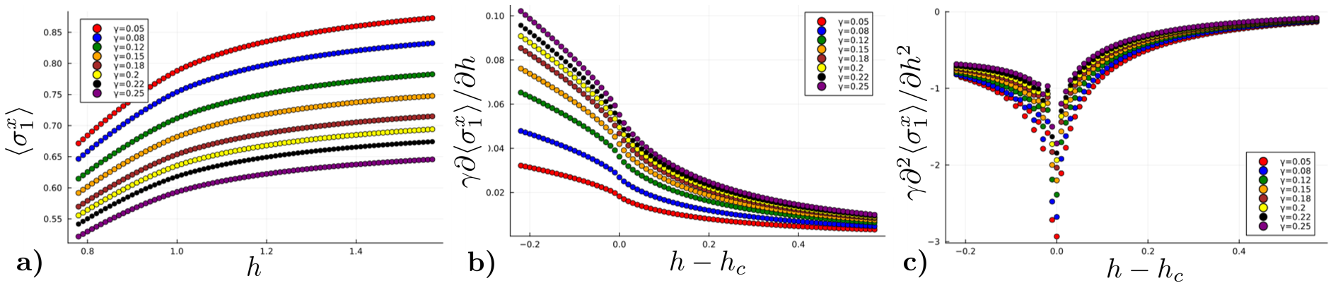
Figure 5: Transverse boundary magnetization (which is proportional to energy current Eq. 133) and its derivatives for different values of $\gamma$ and $h$. For the ground state at $\gamma=0$, a $|h-h_{c}|^{-1}$ singularity occurs in the second derivation. Finite $\gamma$ seems to round off this singularity.

To resolve this mystery, let us try solving the equal-time correlation function in a similar manner to how we did the two-time correlation function. Starting from Eq. 35, we will now show how to rewrite it in terms of a single-particle matrix

$$\tilde{M}=4A-2\gamma\Delta_{1}=\left(\begin{array}[]{cccc}-2\gamma&-2h&0&0\\ 2h&0&-2J&0\\ 0&2J&0&-2h\\ 0&0&2h&\ddots\end{array}\right).$$ (134)

First, note that

$$\tilde{M}\mathcal{C}+\mathcal{C}\tilde{M}^{\dagger} =\left[4A-2\gamma\Delta_{1}\right]\mathcal{C}+\mathcal{C}\left[-4A-2\gamma\Delta_{1}\right]$$ (135)

$$=4\left[A,\mathcal{C}\right]-2\gamma\left\{\Delta_{1},\mathcal{C}\right\}.$$ (136)

Next, note that the diagonal elements of $\mathcal{C}$ always equal to the identity matrix because $\eta_{j}^{2}=1$. The term $4\gamma\Delta_{1}\mathcal{C}\Delta_{1}$ in Eq. 35 only affects diagonal elements to maintain this constraint. Therefore, for the off-diagonal elements $\mathcal{C}_{\text{od}}$,

$$\frac{d\mathcal{C}_{\text{od}}}{dt}=4\left[A,\mathcal{C}_{\text{od}}\right]-2\gamma\left\{\Delta_{1},\mathcal{C}_{\text{od}}\right\}=\tilde{M}\mathcal{C}_{\text{od}}+\mathcal{C}_{\text{od}}\tilde{M}^{\dagger}.$$ (137)

This means that the eigensystem of $\tilde{M}$ determines evolution of the equal-time correlations. If $\tilde{M}$ has a complete set of right eigenvectors $v_{j}$ with non-degenerate eigenvalues $\lambda_{j}$ (the special case of exceptional points can be considered separately if treating the phase transitions), then $v_{j}v_{k}^{\dagger}$ is an eigenmode of the dynamics:

$$\frac{d}{dt}\left(v_{j}v_{k}^{\dagger}\right) =\tilde{M}v_{j}v_{k}^{\dagger}+v_{j}v_{k}^{\dagger}\tilde{M}{}^{\dagger}$$ (138)

$$=\lambda_{j}v_{j}v_{k}^{\dagger}+\lambda_{k}^{\ast}v_{j}v_{k}^{\dagger}-4\gamma v_{j}v_{k}^{\dagger}$$ (139)

We can then use this to calculate the full time evolution. First, note that $C_{\text{od}}$ is strictly imaginary and antisymmetric, while $\tilde{M}^{\prime}$ is real but not symmetric. Therefore, $\tilde{M}^{\dagger}=\tilde{M}^{T}$ implying that $\tilde{M}$ and $\tilde{M}^{\dagger}$ are isospectral and each eigenvalue $\lambda_{j}$ has a partner $\lambda_{j}^{\ast}$:

$$\tilde{M}v_{j}=\lambda_{j}v_{j}\implies v_{j}^{\dagger}\tilde{M}^{\dagger}=v_{j}^{\dagger}\tilde{M}^{T}=\lambda_{j}^{\ast}v_{j}^{\dagger}\implies\tilde{M}v_{j}^{\ast}=\lambda_{j}^{\ast}v_{j}^{\ast}.$$ (140)

For each right eigenvector $v_{j}$, there is also a left eigenvector $w_{j}^{T}$ such that

$$w_{j}^{T}\tilde{M}=\lambda_{j}w_{j}^{T}$$ (141)

A key property is that, while the right eigenvectors $v_{j}$ are not mutually orthogonal, they do form a completeness relation with the left eigenvectors:

$$w_{j}^{T}v_{j^{\prime}}=\delta_{j,j^{\prime}}\Leftrightarrow\sum_{j}v_{j}w_{j}^{T}=\mathds{1}$$ (142)

This allows us to easily decompose the initial correlation function, $\mathcal{C}_{\text{od}}(t=0)$, into eigencomponents:

$$\mathcal{C}_{\text{od},0} =\sum_{j,k}c_{jk}v_{j}v_{k}^{\dagger}$$ (143)

$$w_{j}^{T}\mathcal{C}_{\text{od},0}w_{k}^{\ast} =\sum_{j^{\prime},k^{\prime}}c_{j^{\prime}k^{\prime}}\underbrace{w_{j}^{T}v_{j^{\prime}}}_{\delta_{j,j^{\prime}}}\underbrace{v_{k^{\prime}}^{\dagger}w_{k}^{\ast}}_{\delta_{k,k^{\prime}}}=c_{jk}$$ (144)

Finally, we time evolve to obtain

$$C_{\text{od}}(t)=\sum_{j,k}c_{jk}v_{j}v_{k}^{\dagger}\exp\left[\left(\lambda_{j}+\lambda_{k}^{\ast}\right)t\right]$$ (145)

Like the single Majorana time evolution, this will be dominated by the slowest-decaying modes, namely those with maximum real part of $\lambda_{j}$.

The equal-time evolution matrix $\tilde{M}$ looks very similar to the 2-time evolution matrix $M^{\prime}$ (Eq. 85) with the crucial difference that $\gamma\to-\gamma$. Therefore, when we go to solve for the edge states, the spectrum looks essentially identical except that now the edge mode is the fastest-decaying mode, rather than slowest-decaying. Indeed, due to symmetry of the Hamiltonian under $h\to-h$ and $J\to-J$, the spectrum of $\tilde{M}$ is equal to that of $M$ up to multiplication by overall $-1$ and a constant energy shift, as illustrated in Figure 6. Because the edge modes are now the fastest decaying one, contrary to what occurs for the 2-time correlation function, we do not expect that such edges have an impact in the long-time dynamics of the magnetization. As a consequence, we do expect singularities.

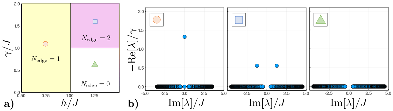
Figure 6: (a) Phase diagram showing number of edge modes for equal-time correlation matrix $\tilde{M}$ (Eq. 134). Note that counting would be the same for $M$, as here we do not restrict to modes that are degenerate at slowest decay. (b) Eigenvalues $\lambda$ of $\tilde{M}$ plotted for three different points in the phase diagram, showing that edge modes are fastest-decaying modes for equal-time correlations.

IX.2 Magnetic susceptibility

Having established that singularities only appear in non-equal-time correlations of the boundary spin, the other observable we consider is boundary magnetic susceptibility $\chi_{B}$, which is related to the 2-time correlation function via the Kubo formula. However, the components occupying these edge states come from equal-time correlations, where edge mode occupation is suppressed as we saw in the previous section. To understand which of these is most relevant, we now solve for magnetic susceptibility numerically.

In order to do so, it is convenient to introduce an additional weak symmetry-breaking magnetic field $h_{B}$:

$$H\to H-h_{B}\sigma_{1}^{z}.$$ (146)

The (zero-frequency) magnetic susceptibility is then

$$\chi_{B}=\lim_{h_{B}\to 0}\frac{\langle\sigma_{1}^{z}\rangle}{h_{B}},$$ (147)

where care must be taken to evaluate this in the same NESS as before. The protocol we choose is as follows:

1. Initialize the system in its ground state at fixed $(h,J,h_{B})$.

2. Quench on $\gamma>0$ and time evolve to $t<L/v$.

3. Plot $\langle\sigma_{1}^{z}\rangle$ as a function of $t$ to obtain the NESS magnetization.

In fact, we can do so efficiently using similar free-fermion numerics by a modified Jordan-Wigner transformation in which an ancillary Majorana $\eta_{0}$ is introduced, as in [35]. The modified mapping is

$$\sigma_{j}^{x}=i\eta_{2j-1}\eta_{2j},\ \sigma_{j}^{z}=i\eta_{0}\left(\prod_{n=1}^{j-1}i\eta_{2n-1}\eta_{2n}\right)\eta_{2j-1}.$$ (148)

While this appears to add interactions to the problem, a similar calculation as before shows that equal-time correlations of the extended Majorana operator vector, $\eta^{T}\equiv\begin{pmatrix}\eta_{0}&\eta_{1}&\eta_{2}&\dots\end{pmatrix}$, are governed by the following single-particle evolution matrices:

$$\frac{\partial\mathcal{C}(t)}{\partial t} =4\left[A_{\text{ext}},\mathcal{C}\right]+\gamma\left[4\left(\Delta_{1}\mathcal{C}\Delta_{0}+\Delta_{0}\mathcal{C}\Delta_{1}\right)-2\left\{\Delta_{0}+\Delta_{1},\mathcal{C}\right\}+4\left(\Delta_{0}+\Delta_{1}\right)\right],$$ (149)

where $\Delta_{j}$ is a diagonal matrix projecting onto the $j$th component and the extended Hamiltonian matrix is

$$A_{\text{ext}}=\begin{pmatrix}0&-h_{B}/2\\ h_{B}/2&0&-h/2\\ &h/2&0&-J/2\\ &&J/2&0&-h/2\\ &&&h/2&0\\ &&&&&\ddots\end{pmatrix}.$$ (150)

Then the boundary magnetization is $\langle\sigma_{1}^{z}(t)\rangle=-i\mathcal{C}_{01}(t)$.

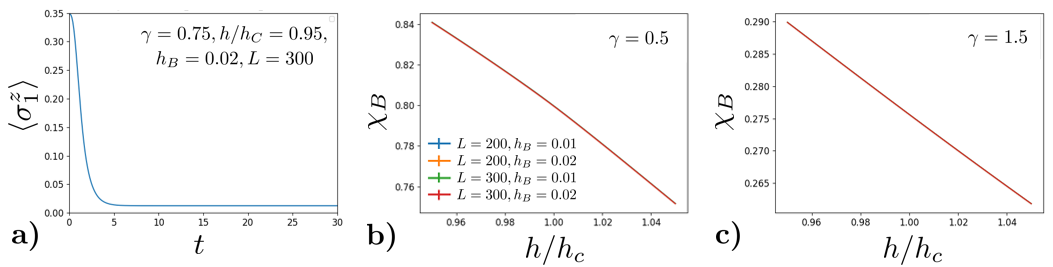
Figure 7: (a) Example of data for longitudinal boundary magnetization, $\langle\sigma^{z}_{1}\rangle$, as a function of time $t$ after a quench from the ground state to finite $\gamma$. (b,c) Boundary magnetic susceptibility obtained from numerical non-equilibrium steady state ($1\ll t<L/v$). Curves various $L$ and $h_{B}$ are nearly identical.

Some examples of the boundary magnetization and susceptibility are shown in Figure 7. Clearly, the system quickly approaches a boundary steady state. However, it is also apparent from lack of finite-size or finite-$h_{B}$ effects near the boundary phase transitions that no low-order singularities exist in the boundary susceptibility. Combined with the previous section, this provides strong evidence that the boundary phase transitions are strictly dynamical phenomena.

X Additional data for interacting model

In this section, we provide additional information and data on the interacting Ising chain and simulations using a variant of time-evolving block decimation (TEBD). The method proceeds by using third quantization (see Section VIII.1) and unfolding the vectorized density matrix to create a one-dimensional problem with dephasing as an impurity in the middle of the chain. Initialization is done by using DMRG to obtain the ground state of $H$, which is then used to initial both the left half of the chain (sites $-L$ to $-1$) and the right half (sites $1$ to $L$). Finally, we quench on the dephasing, which behaves as a non-Hermitian $ZZ$-interaction in the middle of the chain. Finally, the dynamics is solved via conventional TEBD techniques. Below, we provide further analysis of our results.

X.1 Numerical fits for TEBD of non-interacting data

For the non-interacting case ($J_{d}=0$), we know the exact solution and were able to obtain numerical values of $\tau$ from fits of $C(t,\Delta t)$. Therefore, it was surprising when, at first, we were unable to obtain similar quality data for $\tau$ upon fitting $C$ from TEBD. Specifically, as seen in Figure 8, data fitted in the PM phase showed consistent deviations which became stronger upon approaching the critical point.

The solution came from realizing that the analytical solution includes no edge modes in this phase, meaning that $C$ is solely given by the bulk contribution

$$C\sim\int dkc_{k}e^{\lambda_{k}t}$$ (151)

where $c_{k}$ are matrix elements between the initial state and eigenstates of the $M$ matrix and $\lambda_{k}$ are its eigenvalues correspond to the bulk mode with momentum $k$. In the bulk, we have that

$$\lambda_{k}=-2\gamma-i\epsilon_{k}$$ (152)

where $\epsilon_{k}$ is the single-particle dispersion. Factoring out the global decay rate $e^{-2\gamma t}$, we are left with an integral of the form $\int dkc_{k}e^{-i\epsilon_{k}t}$. A similar integral is encountered in solving the boundary spin dynamics of the Ising chain with static boundary field $h_{B}\sigma_{1}^{z}$ [35]. There, we found that a saddle point approximation gives asymptotic decay $\sim t^{-3/2}$ at late times. Applying the same logic to the case with a bulk that is gapped on both the real and imaginary axis, we obtain late time decay $\sim t^{-3/2}e^{-t/\tau}$.

Re-fitting the data using this power law prefactor significantly improves the results, as seen in Figure 8; deviations remain near the critical point, where the power law is expected to change when the bulk goes gapless. Furthermore, the argument of faster decay due to a gapped bulk density of states should also hold for the interacting model at low energy. Therefore, we perform this power-law-dressed fit within the PM phase of the interacting model as well, finding that it decreases the appearance of unphysical jumps in $\tau$. This is the data shown in the main text.

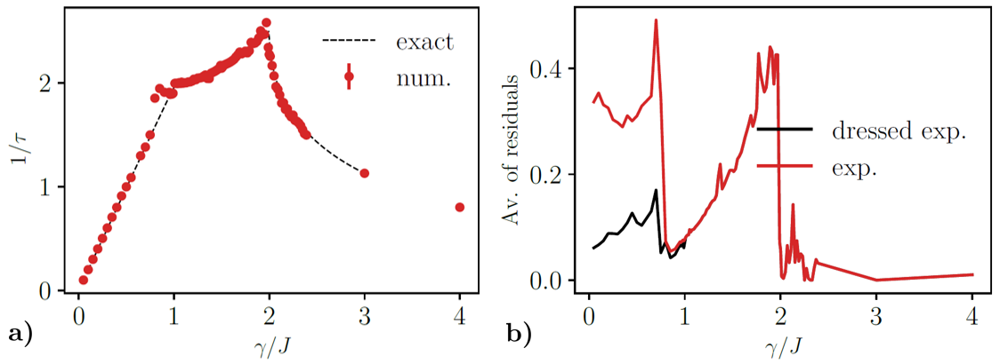
Figure 8: Illustration of improved fitting procedure for 2-time correlation function, applied to free fermions ($J_{d}=0$). (a) Time scale $\tau$ obtained from TEBD simulations of $J_{d}=0$ using the modified fit procedure with power law prefactor $\sim t^{-3/2}$ for data with $h>J$ and $\gamma<J$. (b) Comparison of fit residuals between exponential and exponential with power-law prefactor (“dressed”).

X.2 Alternative integrability-breaking interactions

To confirm robustness of the results for various integrability-breaking interactions, in this section we consider the Hamiltonian

$$H_{xx}=-J\sum_{j}\sigma_{j}^{z}\sigma_{j+1}^{z}-h\sum_{j}\sigma_{j}^{x}+J_{xx}\sum_{j}\sigma_{j}^{x}\sigma_{j+1}^{x}$$ (153)

which also breaks integrability, but without the self-dual interaction that restricts the phase transition to $h=J$. Some data for this are shown in Figure 9. The general behavior is similar to that of the self-dual interaction. Sharp kinks in $\tau^{-1}$ persist, but no longer at the same apparent critical points due to the lack of self-duality. This also causes issues with our fitting procedure, as we manually enforce a power-law-dressed exponential fit for $h>1$ and $\gamma<1$. Since these are apparently no longer the locations of the boundary critical points, a better fitting procedure should be adopted in future work.

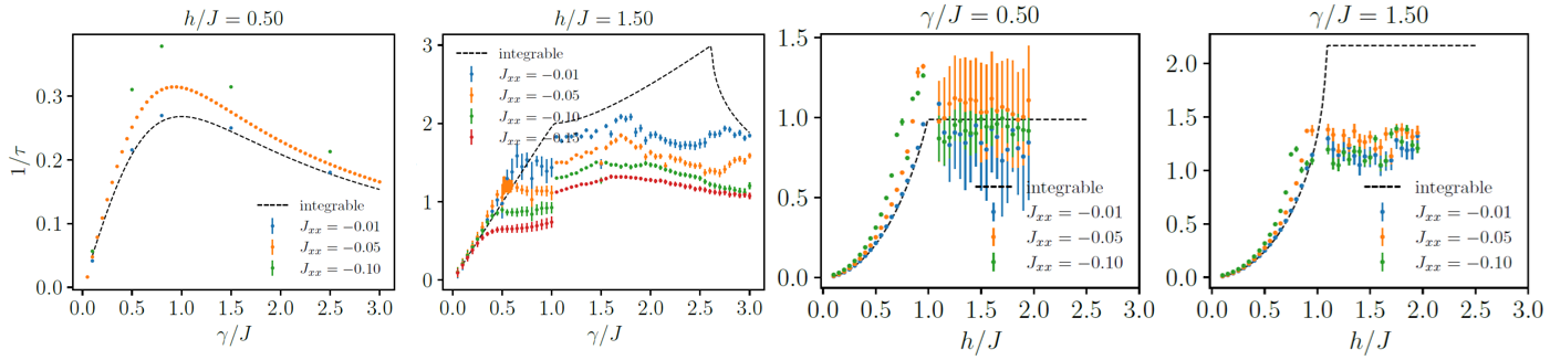
Figure 9: Decay constants for $XX$-interacting Ising chain, obtained by fitting either exponential or power-law-dressed exponential. We force a power-law-dressed fit in $h>1$ and $\gamma<1$ region, resulting in abrupt jumps near this point where the fitting procedure changes.

References

- Langen et al. [2015] T. Langen, R. Geiger, and J. Schmiedmayer, Ultracold atoms out of equilibrium, Annu. Rev. Condens. Matter Phys. 6, 201 (2015).
- Bruzewicz et al. [2019] C. D. Bruzewicz, J. Chiaverini, R. McConnell, and J. M. Sage, Trapped-ion quantum computing: Progress and challenges, Appl. Phys. Rev. 6, 021314 (2019).
- Kjaergaard et al. [2020] M. Kjaergaard, M. E. Schwartz, J. Braumüller, P. Krantz, J. I.-J. Wang, S. Gustavsson, and W. D. Oliver, Superconducting qubits: Current state of play, Annu. Rev. Condens. Matter Phys. 11, 369 (2020).
- Nozieres and De Dominicis [1969] P. Nozieres and C. De Dominicis, Singularities in the x-ray absorption and emission of metals. iii. one-body theory exact solution, Physical Review 178, 1097 (1969).
- Anderson [1967] P. W. Anderson, Infrared catastrophe in fermi gases with local scattering potentials, Physical Review Letters 18, 1049 (1967).
- Silva [2008] A. Silva, Statistics of the work done on a quantum critical system by quenching a control parameter, Physical review letters 101, 120603 (2008).
- Cetina et al. [2016] M. Cetina, M. Jag, R. S. Lous, I. Fritsche, J. T. Walraven, R. Grimm, J. Levinsen, M. M. Parish, R. Schmidt, M. Knap, et al., Ultrafast many-body interferometry of impurities coupled to a fermi sea, Science 354, 96 (2016).
- Knap et al. [2012] M. Knap, A. Shashi, Y. Nishida, A. Imambekov, D. A. Abanin, and E. Demler, Time-dependent impurity in ultracold fermions: Orthogonality catastrophe and beyond, Physical Review X 2, 041020 (2012).
- Tonielli et al. [2019] F. Tonielli, R. Fazio, S. Diehl, and J. Marino, Orthogonality catastrophe in dissipative quantum many-body systems, Physical Review Letters 122, 040604 (2019).
- Kane and Fisher [1992] C. Kane and M. P. Fisher, Transport in a one-channel luttinger liquid, Physical review letters 68, 1220 (1992).
- Kane and Fisher [1995] C. Kane and M. P. Fisher, Impurity scattering and transport of fractional quantum hall edge states, Physical Review B 51, 13449 (1995).
- Latta et al. [2011] C. Latta, F. Haupt, M. Hanl, A. Weichselbaum, M. Claassen, W. Wuester, P. Fallahi, S. Faelt, L. Glazman, J. von Delft, et al., Quantum quench of kondo correlations in optical absorption, Nature 474, 627 (2011).
- Cox and Zawadowski [1998] D. Cox and A. Zawadowski, Exotic kondo effects in metals: magnetic ions in a crystalline electric field and tunnelling centres, Advances in Physics 47, 599 (1998).
- Andrei [1995] N. Andrei, Integrable models in condensed matter physics, in Low-Dimensional Quantum Field Theories for Condensed Matter Physicists (WORLD SCIENTIFIC, 1995).
- McGinley et al. [2017] M. McGinley, J. Knolle, and A. Nunnenkamp, Robustness of majorana edge modes and topological order: Exact results for the symmetric interacting kitaev chain with disorder, Phys. Rev. B 96, 241113 (2017).
- Vasseur et al. [2014] R. Vasseur, J. P. Dahlhaus, and J. E. Moore, Universal nonequilibrium signatures of majorana zero modes in quench dynamics, Phys. Rev. X 4, 041007 (2014).
- Francica et al. [2016] G. Francica, T. J. G. Apollaro, N. Lo Gullo, and F. Plastina, Local quench, majorana zero modes, and disturbance propagation in the ising chain, Phys. Rev. B 94, 245103 (2016).
- Apollaro et al. [2017] T. J. G. Apollaro, G. Francica, D. Giuliano, G. Falcone, G. M. Palma, and F. Plastina, Universal scaling for the quantum ising chain with a classical impurity, Phys. Rev. B 96, 155145 (2017).
- Hu and Wu [2021] K. Hu and X. Wu, First- and second-order quantum phase transitions in the one-dimensional transverse-field ising model with boundary fields, Phys. Rev. B 103, 024409 (2021).
- Campostrini et al. [2014] M. Campostrini, A. Pelissetto, and E. Vicari, Finite-size scaling at quantum transitions, Physical Review B 89, 094516 (2014).
- Campostrini et al. [2015] M. Campostrini, A. Pelissetto, and E. Vicari, Quantum ising chains with boundary fields, Journal of Statistical Mechanics: Theory and Experiment 2015, P11015 (2015).
- Budich et al. [2015] J. C. Budich, P. Zoller, and S. Diehl, Dissipative preparation of chern insulators, PRA 91, 042117 (2015).
- Reiter et al. [2016] F. Reiter, D. Reeb, and A. S. Sørensen, Scalable dissipative preparation of many-body entanglement, PRL 117, 040501 (2016).
- Harrington et al. [2022] P. M. Harrington, E. J. Mueller, and K. W. Murch, Engineered dissipation for quantum information science, Nature Reviews Physics 4, 660 (2022).
- Diehl et al. [2008] S. Diehl, A. Micheli, A. Kantian, B. Kraus, H. P. Büchler, and P. Zoller, Quantum states and phases in driven open quantum systems with cold atoms, Nature Physics 4, 878 (2008).
- Sieberer et al. [2016] L. M. Sieberer, M. Buchhold, and S. Diehl, Keldysh field theory for driven open quantum systems, Reports on Progress in Physics 79, 096001 (2016).
- Rakovszky et al. [2023] T. Rakovszky, S. Gopalakrishnan, and C. von Keyserlingk, Defining stable phases of open quantum systems, arXiv preprint arXiv:2308.15495 (2023).
- Berdanier et al. [2019] W. Berdanier, J. Marino, and E. Altman, Universal dynamics of stochastically driven quantum impurities, Physical review letters 123, 230604 (2019).
- Fröml et al. [2019] H. Fröml, A. Chiocchetta, C. Kollath, and S. Diehl, Fluctuation-induced quantum zeno effect, Physical review letters 122, 040402 (2019).
- Dolgirev et al. [2020] P. E. Dolgirev, J. Marino, D. Sels, and E. Demler, Non-gaussian correlations imprinted by local dephasing in fermionic wires, Physical Review B 102, 100301 (2020).
- Carmichael [2002] H. J. Carmichael, Statistical Methods in Quantum Optics 1 (Springer, 2002).
- Sachdev [2011] S. Sachdev, Quantum Phase Transitions, 2nd ed. (Cambridge University Press, 2011).
- Shibata and Katsura [2020] N. Shibata and H. Katsura, Quantum ising chain with boundary dephasing, Prog Theor Exp Phys 2020, 12A108 (2020).
- Zheng et al. [2023] Z.-Y. Zheng, X. Wang, and S. Chen, Exact solution of the boundary-dissipated transverse field ising model: Structure of the liouvillian spectrum and dynamical duality, PRB 108, 024404 (2023).
- Javed et al. [2023] U. Javed, J. Marino, V. Oganesyan, and M. Kolodrubetz, Counting edge modes via dynamics of boundary spin impurities, Phys. Rev. B 108, L140301 (2023).
- Cardy [1984] J. L. Cardy, Conformal invariance and surface critical behavior, Nuclear Physics B 240, 514 (1984).
- Affleck [1995] I. Affleck, Conformal field theory approach to the kondo effect, Acta Phys. Pol. B 26, 1869 (1995).