Probing the Circumstellar Environment of highly luminous type IIn SN ASASSN-14il

Abstract

We present long-term photometric and spectroscopic studies of Circumstellar Material (CSM)-Ejecta interacting supernova (SN) ASASSN-14il in the galaxy PGC 3093694. The SN reaches a peak $r$-band magnitude of $\sim$ $-20.3\pm 0.2$ mag rivaling SN 2006tf and SN 2010jl. The multiband and the pseudo-bolometric lightcurve show a plateau lasting $\sim 50$ days. Semi-analytical CSM interaction models can match the high luminosity and decline rates of the lightcurves but fail to faithfully represent the plateau region and the bumps in the lightcurves. The spectral evolution resembles the typical SNe IIn dominated by CSM interaction, showing blue-continuum and narrow Balmer lines. The lines are dominated by electron scattering at early epochs. The signatures of the underlying ejecta are visible as the broad component in the H$\alpha$ profile from as early as day 50, hinting at asymmetry in the CSM. A narrow component is persistent throughout the evolution. The SN shows remarkable photometric and spectroscopic similarity with SN 2015da. However, the different polarization in ASASSN-14il compared to SN 2015da suggests an alternative viewing angle. The late-time blueshift in the H$\alpha$ profiles supports dust formation in the post-shock CSM or ejecta. The mass-loss rate of 2-7 M${}_{\odot}\mathrm{yr}^{-1}$ suggests a Luminous Blue Variable (LBV) progenitor in an eruptive phase for ASASSN-14il.

1 Introduction

Core-collapse supernovae (CCSNe) that show narrow (10s to 1000s of km/s) Balmer lines in their spectra are typically classified as type IIn supernovae (hereafter SNe IIn; Schlegel, 1990; Filippenko, 1997). The narrow lines in their spectra arise due to the ejecta of the SN interacting with dense Circumstellar-Material (CSM) surrounding the progenitor (Chugai & Danziger, 1994; Chugai, 2001; Chugai et al., 2004). Early spectra are dominated by a blue continuum, gradually cooling down as the SN evolves. The line profiles are usually multi-component and asymmetric based on the geometry of the explosion. The narrow component (10s to 100s km sec^-1) results from the recombination of ionized unshocked CSM ahead of the blast-wave shock. This usually carries a P-Cygni profile and characterizes the velocity of CSM wind. The intermediate width component (1000s of km sec^-1) arises from the radiation emitted by the Cold-Dense Shell (CDS) region between the forward and the reverse shock and characterizes the velocity at which the blast wave is moving through the CSM (Chevalier & Fransson, 1994). Sometimes, broad components from the underlying explosion, i.e., ejecta signatures, are visible due to diminished interaction or asymmetric CSM geometry (see Smith, 2017 for a review on SNe IIn). These interacting SNe also radiate in X-ray and radio bands in addition to Ultraviolet, Optical, and Infrared. However, the radiation at these wavelengths can be self-absorbed and reprocessed, especially at early times owing to the higher density of CSM (Chevalier, 1982, 1998). Radio and X-ray detections of these events, however, can provide independent constraints on the mass loss of the progenitor. Some SNe IIn also form dust at the later stages of evolution, which leads to IR excess at late times or dust-echoes (Pozzo et al., 2004; Mattila et al., 2008; Fransson et al., 2014; Tartaglia et al., 2020).

SNe IIn are relatively rare ($\sim$9% intrinsic rate among all SNe II; Li et al., 2011) and form a heterogeneous and poorly understood class of transients due to their exceptionally diverse properties. These events have typical absolute magnitudes ranging from M${}_{\mathrm{R}}\sim$ $-16$ to $-19$ mag but some unusually luminous events even reach M${}_{\mathrm{R}}\sim$ $-22$ mag (Kiewe et al., 2012; Taddia et al., 2013; Smith & McCray, 2007). In addition, the overall duration and shape of the lightcurve vary a lot. Some SNe IIn are extremely bright with long-lasting lightcurves (SN 2006gy - Smith et al., 2007; SN 2006tf - Smith et al., 2008); some are slow evolving like (SN 1988Z - Chugai & Danziger, 1994; SNe 2005ip and 2006jd - Stritzinger et al., 2012). Some SNe IIn shows linear decline (SN 1999el - Di Carlo et al., 2002) and some display a plateau (SN 1994W - Dessart et al., 2009; SN 2009kn - Kankare et al., 2012; 2011ht - Mauerhan et al., 2013). Depending on their lightcurve shapes and luminosities, different physical scenarios have been invoked in the literature to explain the powering mechanism of these SNe IIn. A lightcurve powered by ejecta interacting with optically thin CSM can explain moderately bright SNe IIn, but superluminous SNe IIn events require extreme conditions. In order to explain the extreme brightness of SN 2006gy, Smith & McCray (2007) proposed the interaction of ejecta with a compact dense shell as a powering mechanism where the photons diffuse through the optically thick CSM. Woosley et al. (2007) argues that the power source is the collision between shells ejected by a pulsational pair-instability SNe instead. Both these cases point to a very massive progenitor and dense CSM shells. If the CSM shells are extended, they can give rise to the high-luminosities and a relatively slower decline (as seen in SNe 2006tf and 2010jl; Smith et al., 2008; Fransson et al., 2014). Recently, Nicholl et al. (2020) and Suzuki et al. (2021) showed that the lightcurve of SN 2016aps requires a CSM mass $>$ 40M_⊙ to power its luminosity. The dense CSM from the progenitors’ mass-loss events may not extend far. In that case, a transition from an interaction-dominated regime to a Ni-powered regime is seen as similar to SNe IIn-P (Kankare et al., 2012; Mauerhan et al., 2013). However, all these events share the fact that a significant part of the total radiated energy during its lifetime comes from the CSM interaction of ejecta.

Different kinds of progenitor systems can give rise to SNe IIn. They have different CSM profiles (created by the mass-loss events of the progenitor or its binary companion) resulting from these different progenitor systems. SNe IIn typically requires mass-loss rates higher than $10^{-3}\mathrm{M}_{\odot}\mathrm{yr}^{-1}$ (Moriya et al., 2014) which is higher than what can be expected from the line-driven winds (Smith & Owocki, 2006), although SNe IIn falling in the lower range of luminosity can be explained by long-term strong winds (Fransson et al., 2002; Smith et al., 2009a). The enhanced mass-loss from Luminous Blue Variable (LBV) eruptions in months to decades before an SN explosion (Smith, 2014) make them much more suitable progenitor candidates for most SNe IIn. In the case of many SNe, archival images from Hubble Space Telescope (HST) and pre-SN outbursts have revealed their progenitors to be consistent with LBVs (Gal-Yam & Leonard, 2009; Smith et al., 2010, 2011; Kochanek et al., 2011). Additionally, the large amount of CSM required to explain the superluminous supernovae (SLSNe) also favors a massive (40 - 100 M_⊙) LBV progenitor. The outburst in LBVs is still not well understood, but for the more massive LBVs (70-140 M_⊙), it can be due to pulsational-pair instability (Woosley, 2017; Vigna-Gómez et al., 2019). Alternatively, the CSM can result from binary interactions and common envelope ejection. This is usually seen in Ia-CSM type of SNe where a thermonuclear SN explodes within the CSM generated by its companion (SN 2002ic - Benetti et al., 2006; iPTF11kx - Silverman et al., 2013; SNe 2012ca and 2013dn - Fox et al., 2015).

Many authors have developed analytical and numerical modeling frameworks to explain the explosion physics and observables of SNe IIn (Balberg & Loeb, 2011; Svirski et al., 2012; Chatzopoulos et al., 2012; Moriya et al., 2013; Ofek et al., 2014; Dessart et al., 2015; Jiang et al., 2020). Continued observations during the evolution of such events can decipher the mass-loss history decades before the SN explosion, giving crucial insight into the final stages of stellar evolution. In some sense, these interacting SNe are the only real probes to the pre-SN physics of their exotic progenitors. This is especially true at higher redshifts where identifying progenitors using direct imaging is difficult.

In this context, we present the long-term observational photometric and spectroscopic analysis of ASASSN-14il. It was discovered by All Sky Automated Survey for SuperNovae (ASAS-SN) at UT 2014-10-01.11 at $V\sim 16.5$ mag (Brimacombe et al., 2014). The transient was detected in images from the double 14-cm “Cassius” telescope in Cerro Tololo, Chile at RA = 00h45m32.55s, Dec = -14d15m34.6s; approximately 0^′′.33 North and 0^′′.26 West from the centre of the galaxy 2MASX J00453260-1415328. No source was detected at the position of the transient down to the limiting magnitude of $V\sim 17.3$ mag in images taken on UT 2014-09-27.04 and before. Spectroscopic observation on UT 2014-10-03.55 with the Wide Field Spectrograph (WiFeS) mounted on the Australian National University 2.3-m telescope, using the B3000/R3000 gratings ($3500-9800$ Å, $1$ Å resolution) was used to classify the SN (Childress et al., 2014). ASASSN-14il  was classified as a SN IIn based on the narrow emission lines ($\sim$3000 km/s) in the Balmer series and the blue continuum. The redshift calculated from the SN spectrum is consistent with the redshift of the host at 0.022 (Jones et al., 2009). The redshift of 0.022 corresponds to a distance of $88.5\pm 6.2$ Mpc(corrected for Virgo + GA + Shapley) assuming H${}_{0}=73$ km/s/Mpc, $\Omega_{\mathrm{matter}}=0.27$, and $\Omega_{\mathrm{vaccum}}=0.73$. This distance is adopted throughout the paper for further analysis.

The paper is structured as follows. Section 2 describes the observations and data reduction procedures. Estimation of extinction and explosion epoch is discussed in section 3. The lightcurve evolution and modeling in described in sections 4 and 5, respectively. The spectral evolution is described in section 6. Finally, we conclude our paper in section 7 and summarize the results in section 8.

2 Observations and Data Reduction

Table 1: General information about ASASSN-14il and its host galaxy

ASASSN-14il
Discovery Date(1)	UT 2014-10-01.11
Explosion Date	UT 2014-09-25.9
SN Type(2)	IIn
RA (J2000)	00h45m32.55s
Dec (J2000)	-14d15m34.6s
Discovery Magnitude	16.5 mag (V-band)
E(B-V)total	0.21 ± 0.08 mag
Host Galaxy(3)
Galaxy Names	PGC 3093694
	WISEA J004532.52-141532.7
	6dF J0045326-141533
Morphology Type	Dwarf Galaxy
RA (J2000)	00h45m32.601s
Dec (J2000)	-14d15m32.50s
redshift (z)	0.022
vVirgo+Shapley+GA	6462 ± 47 km/s
D	$88.52\pm 6.2$ Mpc
$\mu$	34.74 ± 0.15 mag

References - (1) Brimacombe et al. (2014), (2) Childress et al. (2014),          (3) NED

We observed ASASSN-14il with the Las Cumbres Observatory (LCO) network of telescopes as part of the Supernova Key Project (which eventually became the Global Supernova Project). Observations started from $\sim 2$ days after discovery and continued for over a year with a high cadence in BVgri filters. Since the source was contaminated by the host galaxy, we performed image subtraction using High Order Transform of PSF ANd Template Subtraction (HOTPANTS; Becker, 2015) algorithm integrated in the lcogtsnpipe pipeline (Valenti et al., 2016). The template images were taken in December 2022, long after the SN faded. Figure 1 shows a gri composite image of the science frame, reference frame, and difference image of ASASSN-14il. The BVgri instrumental magnitudes were obtained from the difference images and were calibrated against the AAVSO Photometric All-Sky Survey (APASS) catalog. The photometry of ASASSN-14il is presented in Table 7.

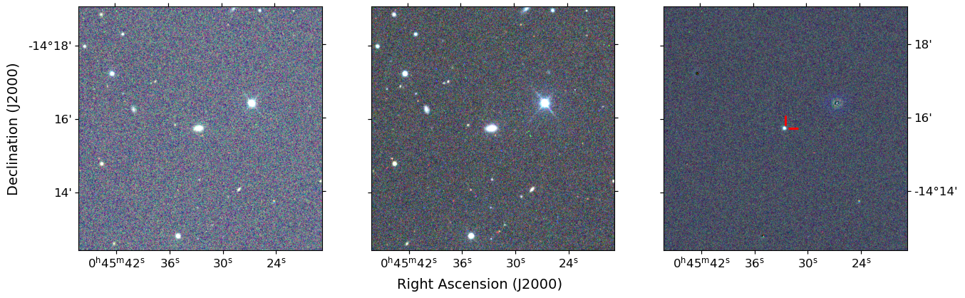
Figure 1: The left panel shows the gri color-composite image of ASASSN-14il with frames taken on 28 November 2014. The central panel shows the gri color-composite with the reference image taken on 27 December 2022, and the right panel shows the color-composite of the difference images with the position of SN marked.

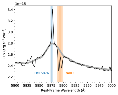
Figure 2: The spectrum of ASASSN-14il showing a prominent dip at 5890 Å and 5896 Å (marked as orange) in the rest-frame of the galaxy indicating high host galaxy extinction. The rest-frame wavelength of the nearby HeI emission line is marked in blue. The grey line shows the continuum used for normalization.

This supernova was also observed using the Ultra-Violet/Optical Telescope (UVOT; Roming et al., 2005) on The Neil Gehrels Swift Observatory (hereafter Swift; Gehrels et al. 2004) in UVW2, UVM2, UVW1, U, B, and $V$ bands starting from day $\sim 8$ to $49$ after the explosion (c.f.r section 3). The photometry was obtained from the Swift Optical/Ultraviolet Supernova Archive (SOUSA; Brown et al., 2014). The reduction is based on that of Brown et al. (2009), which includes subtraction of the host galaxy count rates (from templates taken $\sim$ 2 years after the explosion) using a 5″aperture at the source position, using the revised UV zero points and time-dependent sensitivity from Breeveld et al. (2011). Aperture photometry was performed using an aperture size of 3 or 5 arcsec based on the error. The final UVOT magnitudes are given in Table 8.

Low-resolution (R $\sim$ 400-700) optical spectroscopic observations were carried out using the FLOYDS spectrographs mounted on the LCO 2m telescopes. The 1D wavelength and flux calibrated spectra were extracted using the floydsspec pipeline (Valenti et al., 2014). We include the publicly available data taken under the Public ESO Spectroscopic Survey of Transient Objects (PESSTO) program (Smartt et al., 2015) using EFOSC2 mounted on the 3.6m ESO-NTT. We also include the high resolution (R $\sim$ 3000) spectroscopic data, available in WISeREP (Yaron & Gal-Yam, 2012), which were taken with the Wide Field Spectrograph on the Australian National University 2.3-m telescope under the ANU WiFeS SuperNovA Programme (AWSNAP; Childress et al., 2016). Our optical spectroscopic observations span from day $\sim 8$ to $327$ after the explosion. NIR spectroscopy was acquired using SOFI mounted on the 3.6m ESO-New Technology Telescope (NTT) under the PESSTO program. The NIR observations span from day $\sim 19$ to $\sim 116$. The log of spectroscopic observations is given in Table 9. All the spectra were scaled to photometry by using lightcurve-fitting module (Hosseinzadeh & Gomez, 2022) to account for the slit loss corrections. Finally, all the spectra were corrected for the heliocentric redshift of the host galaxy.

3 Estimation of extinction and explosion epoch

The Milky Way extinction along the line-of-sight of ASASSN-14il is E(B-V)${}_{\mathrm{MW}}=0.0019$ (Schlafly & Finkbeiner, 2011). To estimate the host galaxy contribution to the total reddening, we search for the NaID 5890, 5896 Å doublet in the high-resolution ANU-WiFeS spectra. The NaID doublet is seen at the corresponding host-galaxy rest wavelength. We combine the ANU spectra taken on UT 2014-10-09.50, UT 2014-10-18.56, and UT 2014-10-27.47 to increase the signal-to-noise ratio. The NaID doublet is contaminated by the broad wings of a nearby emission line, as seen in figure Figure 2. Additionally, we note that the HeI emission is blueshifted from its rest wavelength, the implications of which is discussed in section 6. We model the wings of the emission line as a part of the continuum and estimate the equivalent width (EW) of Na D₁ and D₂ from the normalized spectra to be $0.44\pm 0.03$ Å, and $0.57\pm 0.03$ Å, respectively. We use the relation given by Poznanski et al. (2012) between the Na1D features and $E(B-V)$. From this relation, we estimate host galaxy reddening of $0.22\pm 0.09$ mag and $0.21\pm 0.08$ mag, respectively, for D₁ and D₂. We also use the relation for the combined equivalent width of D₁ and D₂ to get the reddening value of $0.22\pm 0.09$ mag, similar to the one estimated individually from D1 and D2. We multiply this reddening value by 0.86 to be consistent with the recalibration of Milkyway extinction by Schlafly & Finkbeiner (2011). Therefore, the host-galaxy extinction is $0.19\pm 0.08$ mag. The fitting errors have been propagated in quadrature. Thus, we adopt a total (galaxy+host) $E(B-V)=0.21\pm 0.08$ mag. We use this value of extinction throughout the paper.

To estimate the explosion epoch of ASASSN-14il, we perform parabolic fitting on the early time $V$-band lightcurve. The magnitudes are converted to fluxes up to 25 days post-discovery. The best-fit coefficients are used to find the roots of the equation, i.e., the value of time for which the flux equals zero. We perform the fit using MCMC simulations to constrain the associated errors. The explosion epoch is estimated to be JD $2456926.4\pm 0.5$ (UT 2014-09-25.9) and adopted as the reference epoch throughout the paper. The general information about ASASSN-14il and its host galaxy is listed in Table 1.

4 Lightcurve Characteristics of asassn-14il

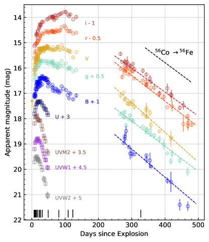
Figure 3: The evolution of optical and UV lightcurves of ASASSN-14il. Different bands are plotted with an offset for clarity. Circles represent the photometry from LCOGT, and squares represent the photometry from Swift UVOT. Epochs having accompanying spectra are represented by line symbols at the bottom. A plateau can be seen in the optical bands between days 40–80. A prominent bump in the lightcurve can be seen around day 90.

Table 2: The rise time and peak magnitudes of UV-Optical bands with a clear peak observed. The listed value and error of Rise Time and Observed Peak Magnitude are derived from the distribution resulting from the MC experiments.

	Rise Time	Peak Magnitude
		Observed	Absolute
	(day)	(mag)	(mag)
UVW2	$14.7\pm 0.9$	$14.54\pm 0.03$	$-22.0\pm 0.7$
UVM2	$15.2\pm 0.9$	$14.43\pm 0.03$	$-22.2\pm 0.7$
UVW1	$17.8\pm 0.8$	$14.30\pm 0.02$	$-21.8\pm 0.5$
U	$21.6\pm 1.2$	$14.32\pm 0.02$	$-21.4\pm 0.4$
B	$36.3\pm 0.5$	$15.57\pm 0.01$	$-20.0\pm 0.3$
g	$38.3\pm 0.3$	$15.18\pm 0.01$	$-20.3\pm 0.3$

Table 3: The lightcurve decline rates in all optical bands at various phases of evolution. The epochs are given with respect to the estimated explosion epoch.

	Time Interval
	40-90d	250-500d
	(mag d-1)	(mag d-1)
B	0.009$\pm$0.002	0.011$\pm$0.001
g	0.004$\pm$0.001	0.010$\pm$0.001
V	0.002$\pm$0.001	0.012$\pm$0.000
r	-0.001$\pm$0.001	0.010$\pm$0.001
i	-0.004$\pm$0.001	0.009$\pm$0.001

The UV and optical lightcurves of ASASSN-14il  are shown in Figure 3. The first $\sim 40$ days after the explosion covers the initial rise in all UV and optical bands. We perform a spline fit on the lightcurves to estimate the peak magnitude and rise times. Monte-Carlo (MC) experiments were done to evaluate the associated uncertainties with the fit. For each MC experiment, we draw pseudo data points from the Gaussian distributions defined by the photometric magnitude and the error bars of the original data points and perform the fit. The rise time and peak magnitudes in UV-Optical bands are listed in Table 2. We observe an increase in the rise time as we move towards the redder bands, which is expected as the photosphere cools down and moves towards redder wavelengths. The lightcurve in Swift UV bands reaches a maximum around day 15-18 and declines very sharply thereafter. The B and g band attains a maximum at around day 36-38, much later than UV bands. The V and r bands do not have a distinct maximum as the initial rising phase directly transitions into a very flat plateau (day 40-100). The i band slowly rises in this duration. The flattening of the optical lightcurves in optical bands between days 60-90 could be due to an ongoing CSM interaction. Both UV and optical lightcurves are bumpy in nature, with the optical bands showing a prominent bump around day 100. These small bumps in the lightcurve can be attributed to SN ejecta encountering regions with enhanced CSM density (Graham et al., 2014). All optical bands show a decline in late phases (day $>250$). The initial decline of the lightcurves after the plateau is not well captured due to data gaps (days 120-260). Therefore, it is not possible to comment on the similarities with the transitional phase of SNe IIn-P. The lightcurve settles into the decline of 1.0-1.2 mag (100d)^-1 at late phases, which is close to the expected ⁵⁶Co decay rate of 0.98 mag (100d)^-1. It is possible to explain the observed decay rate as a result of the ejecta-CSM interaction as well, as this mechanism can give rise to a wide diversity of decay rates in SNe IIn. The lightcurve decline rate in all optical bands at different phases of the evolution is given in Table 3.

4.1 Comparison Sample

Table 4: General properties of the SNe IIn comparison sample. We have taken redshift dependent distances assuming H₀ = 73 km sec^-1 Mpc^-1, $\Omega_{\mathrm{matter}}$=0.27, and $\Omega_{\mathrm{vaccum}}$=0.73. The redshifts are corrected for the effects of GA, Virgo, and Shapley unless mentioned otherwise. We take the reference epoch to be the explosion epoch if available in the literature; otherwise, the discovery epoch is considered.

SN	Host Galaxy	Offset from center	Distance	Extinction	Discovery	Explosion	Reference†
			(Mpc)	$E(B-V)$ (mag)	(mjd)	(mjd)
SN 2005ip	NGC 290	2′′.8 E, 14′′.2 N	33.7	0.047	53679.16	-	1
SN 2006gy	NGC 1260	0.′′941 W,0′′.363 N	77.7	0.56	53996.3	53967.0	2, 3
SN 2006tf	SDSS J124615.80+112555.5	0′′.2 E, 0′′.7 N	330	0.027	54081.0	-	4
SN 2009kn	MCG -3-21-6	17′′.75 E,15′′.27 N	68.9	0.114	55130.5	55115.5	5
SN 2010jl	UGC 5189A	2′′.4 E,7′′.7 N	49.2	0.058	55503.3	55478.6#	6, 7
SN 2011ht	UGC 5460	12′′.4 E,17′′.2 N	20.5	0.061	55833.0	-	8
PTF11oxu	WISEA J033834.32+223242.7	0′′.06 E, 16′′.5 N	376	0.176	55853.3	55837.3	9, NED
PTF11rfr	WISEA J014216.97+291625.6	0′′.19 W, 14′′S	286	0.042	55906.1	55895.4	10, NED
SN 2012ab	SDSS J122247.61+053624.2	0′′.01 E, 0′′.70 N	83.6	0.079	55957.9	55955.3	11
SN 2015da	NGC 5337	12′′.00 E, 14′′.00 N	37.2	0.98	57031.9	57030.4	11, 12
ASASSN-15ua	GALEXASC J133454.49+105906.7	1′′.40E, 0′′.95S	244.5*	0.0578	57368	-	13
SN 2016aps	-	0′′.15	1302*	0.0263	57440.0	-	14
ASASSN-14il	WISEA J004532.52-141532.7	0′′.33 N, 0′′.26 W	88.5	0.24	56931.1	56925.9	This work

^† References: (1) Stritzinger et al. (2012) (2) Smith & McCray (2007); (3) Agnoletto (2009); (4) Smith et al. (2008); (5) Kankare et al. (2012); (6) Jencson et al. (2016); (7) Zhang et al. (2012); (8) Mauerhan et al. (2013); (9) Nyholm et al. (2020); (10) Gangopadhyay et al. (2020); (11) Tartaglia et al. (2020); (12) Smith et al. (2023); (13) Dickinson et al. (2023); (14) Nicholl et al. (2020)
$*$ Distances are not corrected for the effects of GA, Virgo and Shapley.
^# The adopted explosion date is that of the first detection.

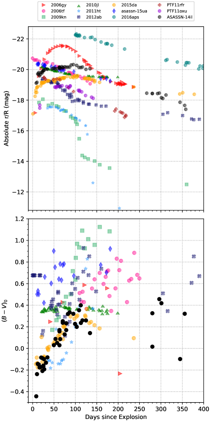
Figure 4: top: Absolute r/R-band lightcurve of ASASSN-14il compared with those of the SNe IIn in the comparison sample. ASASSN-14il is very luminous only dwarfed by SNe 2006gy and 2016aps. The lightcurve is very similar to SN 2015da, but the decline rate of ASASSN-14il is higher than SN 2015da and similar to SNe 2006tf, 2016aps, and ASASSN-15ua. bottom: Intrinsic B-V color of ASASSN-14il compared with the reference sample. The gradual reward evolution of B-V color evolution is similar to SNe IIn.

We have chosen a fairly diverse comparison sample of eleven other well-researched SNe. The sample consists of the following objects: SNe 1998S, 2005ip, 2006gy, 2006tf, 2009kn, 2010jl, 2011ht, PTF11rfr, PTF11oxu, 2012ab, ASASSN-15ua, and 2016aps. These are strongly interacting SNe IIn, covering a diverse range in luminosity, and show interaction signatures up to late times. The basic parameters of the comparison SNe are laid out in Table 4. SNe 2005ip and 2012ab represent the normal luminosity SNe IIn. SNe 2006gy, 2006tf, 2010jl, ASASSN-15ua, and 2016aps are all very luminous type SNe IIn having peak M${}_{r/R}<-20$ that result from various CSM configurations. SNe IIn-P 2009kn and 2011ht, with a distinct plateau in their lightcurves, are also included in this comparison sample. As noted by Nyholm et al. (2020), PTF11rfr and PTF11oxu also show a plateau in their lightcurve, but unlike the SNe IIn-P, they don’t show a sharp drop from the plateau into a ⁵⁶Ni-dominated tail. The lightcurve modeling of these SNe reveals a diversity in their CSM configuration. SN 2006gy results from a massive compact CSM shell (Smith & McCray, 2007), while more extended CSM structures power the comparatively long-lived lightcurves of SNe 2006tf, 2010jl, and ASASSN-15ua (Smith et al., 2008; Ofek et al., 2014; Dickinson et al., 2023).

We have compiled a sample containing the normal luminosity and very luminous SNe IIn from the literature. Also, the different lightcurve shapes resulting from different physical scenarios enable us to highlight the lightcurve heterogeneity of SNe IIn and the role of CSM interaction in their photometric evolution. The sample allows us to put the luminosity of ASASSN-14il  in perspective and infer the possible physical scenario by comparing and contrasting their lightcurve and color evolution.

4.2 Absolute lightcurve and Color Evolution

Adopting the distance modulus $\mu=34.74\pm 0.15$ mag and total reddening $E(B-V)=0.21\pm 0.08$ mag, we generate the absolute magnitude lightcurves of ASASSN-14il. The $r$-band magnitude of ASASSN-14il  plateaus at $\sim-20.2$ mag over many tens of days. The $V$-band also shows similar behavior. Figure 4 shows the comparison of the absolute $r$-band lightcurve of ASASSN-14il with other SNe from the comparison sample. ASASSN-14il stands out as one of the most luminous SN in the comparison sample, which is in concordance with SNe 2006tf, ASASSN-15ua, 2010jl and is only dwarfed by the extremely luminous SNe 2006gy and 2016aps. The lightcurve shape of ASASSN-14il is very similar to SN 2015da except at the late epochs when SN 2015da declines much more slowly. However, the decline rate of ASASSN-14il is similar to those of SNe 2006tf, ASASSN-15ua, and 2016aps. The lightcurves of all these SNe were powered by massive amounts (in order of tens of M_⊙) of dense extended CSM structures that allow the ejecta-CSM interaction to persist until late times (Smith et al., 2008; Dickinson et al., 2023; Tartaglia et al., 2020; Smith et al., 2023; Nicholl et al., 2020). The progenitors for these events that can provide the required mass-loss are speculated to be massive LBVs. A similar progenitor and physical scenario seems plausible for explaining the observed luminosities and late-time decline rate of the lightcurves of ASASSN-14il as well.

SNe IIn-P 2009kn and 2011ht show a plateau in their lightcurve, but afterward, they steeply drop into a radioactivity-dominated tail. On the other hand, SNe like PTF11rfr and PTF11oxu show a plateau in their lightcurve, but their lightcurves smoothly decline afterward in the $r$-band (Nyholm et al., 2020). Due to the data gaps between days 120-260, it is not possible to establish parallels with either of these classes of objects. However, we note that the SNe IIn-P in our sample are generally much fainter than ASASSN-14il.

The B-V color evolution of ASASSN-14il is in agreement with the other SNe IIn from the comparison sample. All the SNe show a redward evolution in the B-V color as the photosphere cools down, ASASSN-14il maintains an overall bluer color. The overall color evolution of ASASSN-14il is strikingly similar to SN 2015da.

After correcting the multi-band magnitudes obtained for extinction, the flux integration (in UVW2, UVM2, UVW1, U, B, g, V, r, i bands) was performed with blackbody corrections to attain the bolometric luminosities using SuperBol (Nicholl, 2018). The lightcurve peaks at day $\sim$16 attaining a luminosity of $1.6\times 10^{44}$ erg s^-1. Gal-Yam (2012) suggested that SNe showing peak magnitude less than –21 in any band or peak luminosity higher than $7\times 10^{43}$ erg s^-1 may be considered as SLSNe. According to both these criteria, ASASSN-14il  can be considered as a SLSNe; however, this threshold is somewhat arbitrary, as mentioned in Gal-Yam (2019), and it is unclear whether two separate luminosity populations exist for SNe IIn.

Table 5: Fitting parameters for MOSFiT csm and csmni models. The shell and wind type CSM are represented by ‘s0’ and ‘s2’ suffixes, respectively.

Model	Mej	vej	fNi	MNi	Mcsm	R0	log $\rho_{0}$	$\dot{M}$	tcsm
	(M⊙)	(km s-1)	(%)	(M⊙)	(M⊙)	(AU)	(g cm-3)	(M⊙ yr-1)	(yr)
csm_s0	$32.2^{+6.1}_{-5.7}$	$4654.4^{+171}_{-162}$	-	-	$9.1^{+1.9}_{-1.4}$	$102.4^{+22.3}_{-17.2}$	$-10.8^{+0.1}_{-0.1}$	-	4.8
csm_s2	$108.4^{+5.8}_{-5.3}$	$4685^{+97}_{-124}$	-	-	$4.7^{+0.3}_{-0.3}$	$19.8^{+4.2}_{-2.9}$	$-10.8^{+0.1}_{-0.1}$	2.8	0.9
low_Ni+csm_s0	$20.9^{+16.7}_{-12.8}$	$4670^{+210}_{-200}$	$0.4^{+0.3}_{-0.2}$	$0.08^{+0.18}_{-0.07}$	$15.87^{+12.53}_{-5.73}$	$187.11^{+145.4}_{-68.2}$	$-10.43^{+0.7}_{-0.3}$	-	8.9
low_Ni+csm_s2	$14.6^{+2.7}_{-2.6}$	$4897^{+172}_{-111}$	$8^{+0.5}_{-0.5}$	$1.2^{+0.3}_{-0.3}$	$5.4^{+0.8}_{-1.0}$	$80.2^{+13}_{-16}$	$-10.36^{+0.11}_{-0.16}$	125.3	3.8
high_Ni+csm_s0	$6.93^{+0.6}_{-0.5}$	$5370^{+253}_{-241}$	$66^{+5}_{-6}$	$4.6^{+0.8}_{-0.7}$	$1.9^{+0.7}_{-0.5}$	$87.76^{+22.1}_{-14.5}$	$-11.87^{+0.03}_{-0.02}$	-	4.2
high_Ni+csm_s2	$7.6^{+0.6}_{-0.4}$	$6025^{+284}_{-271}$	$65^{+4}_{-5}$	$4.9^{+0.7}_{-0.6}$	$3.2^{+0.4}_{-0.3}$	$126^{+16}_{-15}$	$-12.1^{+0.1}_{-0.!}$	5.63	5.97

5 multi-band lightcurve modeling using MOSFiT

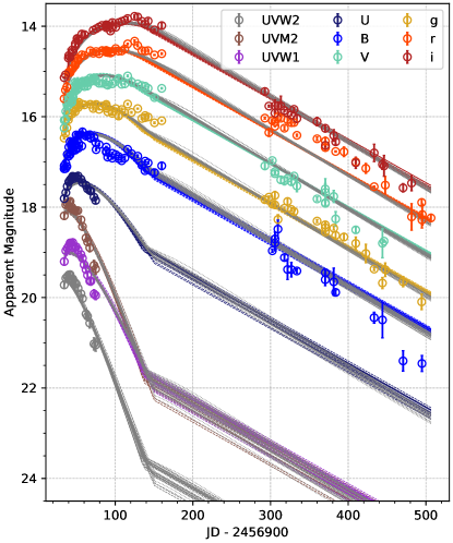
Figure 5: Results of csm models from MOSFiT. The lightcurves representative of the evaluated posterior are plotted on top of the observational data. The colored and gray lines represent the posterior of wind and shell csm models, respectively. The lightcurves of ASASSN-14il are well reproduced by the CSM models with M_csm between 5-9 M_⊙.

To estimate the physical parameters associated with the explosion, we also performed analytical multi-band lightcurve modeling of ASASSN-14il. MOSFiT is an open-source lightcurve fitter for transients (Guillochon et al., 2018). It fits the multiband lightcurves with a list of built-in models using Markov Chain Monte Carlo (MCMC) methods.

Since narrow and intermediate width lines, which are indicative of interaction, are seen in the spectra of ASASSN-14il throughout its evolution, we attempted to fit its lightcurves with the models which include CSM as a powering mechanism. Chevalier (1982, 1998) lays the analytical groundwork for the radiation expected from ejecta interacting with CSM. To achieve a self-similar solution, it is assumed that the ejecta is expanding gas into a stationary CSM. Both the expanding outer-ejecta and the stationary CSM are assumed to follow a power-law distribution ($\rho_{\mathrm{ejecta}}\propto r^{-n}$ and $\rho_{\mathrm{CSM}}\propto r^{-s}$). Chatzopoulos et al. (2012) presented generalized semi-analytical models that take into account shock power from interaction, magnetar spin-down, and ⁵⁶Ni radioactivity. This work has been used in Chatzopoulos et al. (2013) with $\chi^{2}$-minimization algorithm to find optimal parameters for a sample of interacting SNe. Chevalier (1982) presented the solutions for $s=0$ and $s=2$ and later Jiang et al. (2020) extended these solution to $0\leq s\leq 2$. This model, along with a generalized framework to easily fit multiband lightcurves, is implemented in MOSFiT.

In the MOSFiT csm model, it is assumed that the SN luminosity results from the conversion of kinetic energy from both the forward and reverse shock into heating. While in the csmni model, ⁵⁶Ni is considered as an additional power source along with the csm interaction. We fitted the lightcurves of ASASSN-14il  with both the csm and csmni models. We fix the power law index of the outer ejecta $n=12$, which is expected for the explosions of RSGs (Matzner & McKee, 1999; Moriya et al., 2013). We fix the opacity $k=0.34$ cm² g^-1 for fully ionized hydrogen-rich material. We take the rest of the parameters as fitting parameters. The fitting was performed using the dynamic nested sampler dynesty (Speagle, 2020). For ejecta mass and csm mass, we consider uniform priors from 1-150 M_⊙. For the inner radius of CSM (R₀), we consider a uniform prior from $1-500$ AU, and for the CSM density at the inner radius ($\rho_{0}$), we consider a log-uniform prior from $10^{-14}-10^{-9}$ g cm^-3. From both csm and csmni cases, we fitted with a shell csm ($s=0$) and a wind csm ($s=2$) models. For the low_Ni and high_Ni models we consider a uniform prior from 0.1-10% and 0.1-100% for the nickel fraction in ejecta (f_Ni = M_Ni / M_ej), respectively. The estimated parameters from fitting various models are listed in Table 5. The $1\sigma$ errors listed represent the statistical uncertainty associated with fitting and hence are not indicative of the model uncertainties.

Both the csm and csmni models (with either a wind or shell CSM configuration) provide a very similar fit to the observed lightcurves, despite the latter being the more complex. Both are able to reproduce the broad lightcurve features reasonably well. However, these models have a smooth CSM distribution, and therefore they are unable to reproduce both the lightcurve bumps and the decline of lightcurve in the UV bands after the peak. We tried to model the lightcurve after removing the bump seen around day 90, in a manner similar to Hosseinzadeh et al. (2022), but this approach doesn’t improve the fit to the lightcurves in our case. Figure 5 shows the sample lightcurves for the csm (shell and wind) models, which are representative of the posterior for these models. The late-time luminosity is powered by the reverse shock running through the ejecta after the forward shock terminates. The models having an extremely high fraction of ⁵⁶Ni in the ejecta can reproduce the steep decline of UV lightcurves. But due to their unphysical nature, we neglect these models. The variation of the estimated parameters for different models dominates over the fitting uncertainties. However, the requirement of a high ejecta mass (10–100 $M_{\odot}$) and a very dense CSM ($\sim 10^{-11}$ g cm^-3) are consistent.

The mass-loss rate for the wind-like csm models is calculated as $\dot{M}=4\pi v_{w}\rho_{0}R_{0}^{2}$, and the time of ejection of CSM (t_csm) is calculated as $R_{0}/v_{w}$, where we have assumed a typical LBV-like wind velocity ($v_{w}$) of 100 km sec^-1. We estimate a mass-loss rate of 2.8 M_⊙ yr^-1 (for the csm_s2 model), and the CSM shell/wind expelled about 1-5 years prior to the explosion.

6 Spectroscopic Evolution

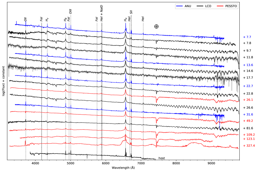
Figure 6: Spectral Evolution of ASASSN-14il from day 8–327. Spectra are displayed in the source rest frame and are corrected for extinction. The grey color represents the original spectra, and the colored lines represent smoothed spectra. Early spectra have a blue continuum and narrow H and He lines with Lorentzian wings. Broad ejecta components can be seen in H$\alpha$ and H$\beta$ lines along with intermediate width lines at later epochs. The host spectrum is plotted at the bottom.

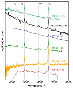
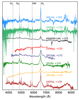
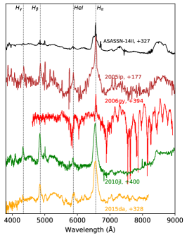
Figure 7: Comparison of ASASSN-14il spectra with the comparison sample at distinct stages of its evolution. SNe IIn-P and SNe IIn are plotted above and below the spectra of ASASSN-14il (black). ASASSN-14il shows prominent Balmer features from early times similar to other SNe IIn and SNe IIn-P. At mid epochs, the Balmer lines are much more prominent in the SNe IIn-P owing to their weaker continuum, in contrast to the SLSNe. At late epochs, many of the SNe develop a noticeable blueshift in their H$\alpha$ profiles.

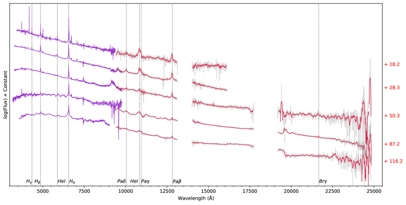
Figure 8: NIR spectral evolution of ASASSN-14il. The NIR spectra are plotted along with optical spectra from nearby epochs. The spectra are displayed in the source rest frame and are not corrected for reddening. The gray color represents the original spectra, and the colored lines represent smoothed spectra. The evolution of Pashcen lines is similar to the optical Balmer lines.

The spectral evolution of ASASSN-14il from day $\sim$8–327 is shown in Figure 6. From the first spectra, narrow line features of Hydrogen are visible, which contrasts with some SNe IIn, where initial spectra are almost featureless. The overall spectral evolution is very slow. Multicomponent H$\alpha$ line is visible throughout its spectral evolution. Other Balmer lines, as well as weak He lines (5876, 6678, and 7065 Å) are also present since the beginning. The evolution of H$\alpha$ is very smooth, and a detailed description is given in subsection 6.2. The lines originating from SN ejecta like Ba II, Sc II, Mg I, Ti II, and Ca II that are usually seen in a normal CCSNe without predominant interaction are not visible in the early phase of spectral evolution. Some lines like O III and S II are seen in the spectral evolution, indicating contamination by the host galaxy. For comparison, we have also shown the host-galaxy spectrum in Figure 6. The host galaxy spectrum was taken on UT 2004-09-06.61 under the 6dF galaxy survey (Jones et al., 2004, 2009).

The first spectrum was taken on day 8, featuring a blackbody continuum at a temperature of 11,000 K and a radius of 100 AU. This spectrum shows narrow H$\alpha$ profiles on top of smooth Lorentzian wings. Similar Lorentzian wings are present in other Balmer and He lines. The N II contamination from the host galaxy is also seen in this spectrum.

The spectra are dominated by Lorentzian line profiles and a smooth blue continuum up to day 30. At day 50, the line profile slowly shifts from Lorentzian into more complex multi-component profiles. During this time, the temperature of the continuum decreases to 6000 K and becomes constant thereafter. After day 50, ejecta signatures are visible as a broad component in the H$\alpha$ line.

After day 100, a clear blueshift can be noticed in the H$\alpha$ profile, the extent of which increases with time. At day 327, the Balmer lines are dominated by the broad ejecta component, and CaII (both forbidden and NIR) lines are also visible. The blueshift seen earlier is even more prominent at this stage. The nebular phase spectral lines typical for the CCSNe are not visible at these later stages either. The systematic blueshift in the H$\alpha$ profile can arise due to the asymmetric CSM or dust formation in the post-shock gas (Smith et al., 2008; Jencson et al., 2016).

The narrow emission feature of the HeI 5876 Å line is noticeably redshifted compared to the rest-wavelength in the higher resolution ANU spectra (taken between day 8-32; Figure 2). Such a redshift can be caused by an unresolved P-cygni profile characteristic of a CSM outflow (Smith et al., 2023). The blue-edge of the narrow P-Cygni in SN 2017hcc lies at -70 to -60 km s^-1, which is completely washed out in low to moderate resolution spectra (Smith & Andrews, 2020). ASASSN-14il maybe a similar case where the P-Cygni profile in HeI and corresponding narrow P-cygni profiles in Balmer lines are unresolved due to the limited resolution of the spectra. It is also possible that these narrow P-Cygni features are masked due to contamination from the host.

Comparison of ASASSN-14il spectra with other SNe IIn from the comparison sample at different stages of its evolution is shown in Figure 7. All the SNe have a blue continuum in the early spectrum (day $\sim 20$). All interacting SNe show narrow emission lines superimposed on the continuum. The H$\alpha$ of ASASSN-14il is very prominent, similar to most of the SNe in the comparison sample signifying strong ongoing interaction. However, SN 2012ab exhibits relatively weaker H$\alpha$, which results from directly seeing the high-velocity jet-like ejecta with relatively lesser CSM interaction at this phase (Gangopadhyay et al., 2020). The early spectra of ASASSN-14il bear an overall resemblance to the other events in the sample except for SN 2005ip, which shows a spectrum similar to normal type II, with narrow lines from preshock CSM on top (Smith et al., 2009b).

The spectral evolution of ASASSN-14il at mid-phases closely resembles SNe 2006gy and 2015da around day $\sim$ 120. SN 2010jl has similar H$\alpha$ line morphology but with more prominent Balmer lines than ASASSN-14il. This spectral synergy between the three SNe is also evident in their photometric behavior, showing high luminosities and long-lasting lightcurves. In contrast, for the SNe IIn-P 2009kn and 2011ht, H$\alpha$ line emission is more prominent with respect to their weaker continuum. In addition to the narrow component, a broad component can be clearly seen in ASASSN-14il  and all the other SNe IIn. This component arises due to the ejecta contribution in the H$\alpha$ profile. Additionally, the broad component of ASASSN-14il shows a deficit in the red side flux of the H$\alpha$ line similar to SNe 2005ip, 2010jl, and 2015da.

After $\sim 1$ year of the explosion, ASASSN-14il shows a flat-topped broad component in H$\alpha$, with the narrow component on top. The observed blueshift in ASASSN-14il and SNe 2005ip, 2010jl, and 2015da is much more prominent compared to the mid-phases. The overall blueshift in the line profile of SN 2010jl was interpreted as the broadening due to electron scattering (Fransson et al., 2014). However, Smith et al. (2012, 2023) argue that broadening by electron scattering should be symmetric about the original source of the narrow-line photons. The narrow lines in SNe 2010jl and 2015da are found at rest-frame velocities even at late phases where a blueshift is seen in the H$\alpha$ profile. Instead, this blueshift is explained as a result of dust formation in the post-shock CSM/ejecta, which preferentially blocks the emission from receding material, which is consistent with the other evidence of dust-formation (Maeda et al., 2013; Gall et al., 2014). The H$\alpha$ profile of ASASSN-14il also shows an overall blueshift and a rest-frame emission component. The H$\alpha$ profile of ASASSN-14il at this epoch is similar to SN 2005ip at day $\sim 177$, which shows a similar blueshifted flat top profile. This blueshifted profile appears in SN 2005ip as early as day $\sim 120$ and is attributed to the post-shock dust formation in the CDS (Fox et al., 2009; Bak Nielsen et al., 2018). Based on these comparisons, the blueshifted H$\alpha$ profile of ASASSN-14il is likely the result of dust formation in the post-shock CSM/ejecta.

6.1 Infrared Spectrum

Five NIR spectra were obtained for ASASSN-14il between days 19–116 after the explosion. They are displayed in Figure 8 along with the closest optical spectra. Prominent lines of Pa$\alpha$, Pa$\beta$, and Pa$\delta$ can be seen in the spectral sequence of ASASSN-14il. Pa$\gamma$ is also visible but is usually blended with He i 10830 Å and Pa$\epsilon$ line. The FWHM of the Pa$\beta$ and Pa$\delta$ typically varies between 8,000 - 13,000 km sec^-1. The lines here are isolated, and FWHMs concord with H$\alpha$ within error bars. Overall, the NIR spectra of ASASSN-14il are consistent with optical spectra regarding interaction features, mostly implied from the FWHM’s being consistent in both the wavelength regimes.

6.2 H-alpha Evolution

ASASSN-14il suffers significantly from host galaxy lines of OII, NII, and SII (seen clearly in the higher resolution WiFeS spectral sequence). The host-galaxy spectrum taken under the 6dF survey (see section 6) has an FWHM resolution of 9–12 Å in the H$\alpha$ region. The SN spectra have lower resolution compared to the host spectrum. The SN spectrum was subtracted after degrading the resolution of the host galaxy spectrum, taking the SII 6717-6731 Å line as a reference for host contribution. In most low to medium-resolution spectra, the host galaxy contribution is almost removed, leaving an unresolved narrow residual component behind. For the ANU-WIFES spectra, the analysis was performed as is, without performing the host-galaxy subtraction, as they are much higher in resolution than the available host spectra.

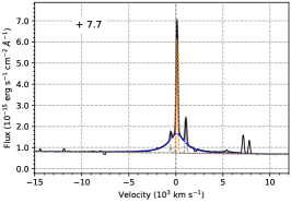
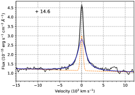
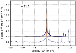
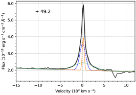
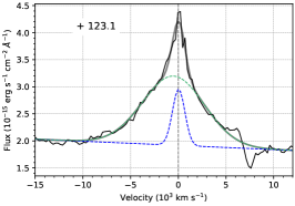
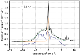
Figure 9: The H$\alpha$ evolution of ASASSN-14il being fitted with multiple Lorentzian and Gaussian components. The host galaxy contribution is subtracted, and the continuum is selected by masking the line regions. ASASSN-14il shows a very complex geometry of the spectral profiles. The orange, blue, and green components represent the narrow, intermediate, and broad components, respectively. For day 31.6 and 327.4 The H-beta (violet) from is plotted in violet.

Table 6: This table describes the spectral decomposition of H$\alpha$ profile of ASASSN-14il. The line centers and FWHMs of the narrow, intermediate-width, and broad components are reported.

Phase	Source	Narrow Component		Intermediate-width Component		Broad Component
		center	fwhm	center	fwhm	center	fwhm
(d)		(km s-1)	(km s-1)	(km s-1)	(km s-1)	(km s-1)	(km s-1)
7.7	ANU	131.5$\pm$0.3	190.6$\pm$0.9	96.7$\pm$9.6	2039.4$\pm$27.6	-	-
7.8	LCO	-128.1$\pm$5.3	542.2$\pm$18.2	-54.0$\pm$10.2	1890.1$\pm$55.6	-	-
9.7	LCO	-23.0$\pm$4.7	677.3$\pm$16.6	18.2$\pm$10.0	2196.4$\pm$61.3	-	-
11.8	LCO	37.7$\pm$8.4	628.7$\pm$28.6	113.4$\pm$24.5	2360.8$\pm$129.1	-	-
13.6	ANU	148.3$\pm$0.3	190.8$\pm$0.8	144.9$\pm$8.0	2112.6$\pm$22.7	-	-
14.6	LCO	28.7$\pm$6.1	701.6$\pm$21.8	58.2$\pm$14.3	2239.2$\pm$89.5	-	-
17.7	LCO	72.5$\pm$17.3	568.0$\pm$58.6	-30.9$\pm$26.6	1680.0$\pm$151.3	-	-
22.7	ANU	136.7$\pm$0.3	198.9$\pm$0.9	134.4$\pm$8.3	1949.5$\pm$24.1	-	-
22.8	LCO	-9.4$\pm$4.1	755.4$\pm$12.1	153.8$\pm$27.3	3837.7$\pm$79.5	-	-
26.1	PESSTO	193.6$\pm$8.5	460.0$\pm$28.7	89.1$\pm$11.0	1784.7$\pm$51.9	-	-
26.6	LCO	38.1$\pm$5.0	688.4$\pm$17.7	92.2$\pm$12.9	2090.0$\pm$82.1	-	-
31.6	ANU	144.7$\pm$0.3	178.1$\pm$0.9	130.2$\pm$8.2	1701.7$\pm$24.7	-	-
49.2	PESSTO	239.6$\pm$4.8	497.3$\pm$17.3	118.3$\pm$12.8	1549.7$\pm$57.1	339.0$\pm$69.6	5010.3$\pm$243.0
81.6	LCO	206.8$\pm$1.6	506.3$\pm$5.6	174.3$\pm$6.3	1841.0$\pm$28.9	-973.3$\pm$70.5	8680.9$\pm$241.4
109.2	PESSTO	66.3$\pm$7.6	715.4$\pm$29.4	-59.5$\pm$29.3	2098.5$\pm$130.8	-573.2$\pm$57.3	8197.7$\pm$192.6
123.1	PESSTO	-	-	44.0$\pm$27.9	1531.5$\pm$82.9	-461.2$\pm$52.4	7608.1$\pm$155.3
327.4	PESSTO	-39.6$\pm$9.7	526.5$\pm$24.5	-	-	-957.0$\pm$68.7	6543.2$\pm$165.0

In the host-galaxy subtracted spectra, the H$\alpha$ profile was fitted with combinations of the following to reproduce the overall line profile - i) A narrow Gaussian component, ii) A Lorentzian/Gaussian intermediate width component, iii) A broad Gaussian component. At early times, the overall H$\alpha$ profile is better represented by a Lorentzian intermediate width component as the emission lines are dominated by electron scattering. At late times (day $>$50), a Gaussian intermediate width component better reproduces the overall line profile as the lines evolve into a more complex multi-component structure. The choice of the continuum is very critical for performing these fits. The continuum is selected to be far from the line region by at least 50 Å. The continuum selection was performed repetitively to optimize the consistency of the fits. The spectral evolution and the corresponding fits at selected epochs are shown in Figure 9. The parameters of components obtained from the fitting at all epochs are given in Table 6. The errors listed represent only fitting errors, and other uncertainties like resolution matching, subtraction of host-spectra, and imperfections in wavelength calibration have not been included. The evolution of the line centers and FWHMs of the various components is plotted in the top panel of Figure 10.

Three components can describe the line profiles: i) A narrow component (unresolved in the lower resolution spectra) centered around the rest wavelength, ii) An intermediate width component centered around the rest wavelength, with FWHM typically varying between 1600–2000 km sec^-1, and iii) A broad emission varying in FWHM between 5000–8500 km sec^-1 seen after day 50. This broad component progressively develops a blueshift of $\sim 600-1000$ km s^-1. The minimum FWHM of the narrow component is 178 km sec^-1 seen in the ANU spectra (day 31.6), however it still may be unresolved. To check whether the narrow component seen in the high-resolution ANU spectrum is due to the host or intrinsic to ASASSN-14il, the host-galaxy spectrum was subtracted by degrading the resolution of the ANU spectrum. A residual narrow component persists, indicating narrow line emission from the SN as seen in our spectral sequence. Dickinson (2021) performed a similar analysis with the high-resolution spectrum taken after the SN had faded and arrived at a similar conclusion. It should be noted that this residual narrow component may still be from the host galaxy as the H to N emission ratio is variable depending on the slit positions and orientation. However, a strong narrow component is seen in the HeI $5876$ Å line as well, in spite of the host galaxy having very low HeI emission.

Figure 10: Top Panel: The FWHMs of the different components of the H$\alpha$ obtained by fitting Gaussian/Lorentzian to line profiles. The three color-coded zones in the panels demarcate the regions where ASASSN-14il enters into three phases of its evolution as described in subsection 6.2; Middle Panel: the line flux ratios of H$\alpha$ and H$\beta$ for long-lasting SNe IIn. 10$\%$ error has been included in the flux-ratios; Bottom Panel: the line-luminosity variations of H$\alpha$ as compared with other members of the sub-class.

The H$\alpha$ evolution of ASASSN-14il can be divided into three distinct phases. From day 8–50, the H$\alpha$ is dominated by Lorentzian wings caused by the electron scattering of narrow line photons. A narrow component is also visible in the spectra even after subtracting the host galaxy contribution. This indicates that the photosphere lies in the unshocked CSM at this phase. The UV (and bolometric) lightcurves peak during this phase (around day 15), which can ionize the unshocked CSM. During this phase, no signatures of underlying ejecta are seen in the H$\alpha$ profile, unlike some SNe where broad emission or broad P-Cygni profiles are seen from early times, which would indicate direct line-of-sights to the ejecta. In SN 2012ab, this is achieved by disk-like CSM (Gangopadhyay et al., 2020) and in SN 2005ip, a clumpy CSM structure is present (Smith et al., 2009b).

From day 50–80, the combination of a narrow Gaussian and a Lorentzian profile can no longer accurately reproduce the line profiles. Instead, the line profiles are more faithfully represented by combining three Gaussian (narrow, intermediate width, and broad) components. The broad wings of high-velocity ejecta are distinguishable in the line profiles. The Gaussian intermediate width and broad with components have FWHMs of 1550–2000 km s^-1 and 5000–8000 km s^-1, respectively. No significant P-Cygni absorption associated with the broad H$\alpha$ component is visible, suggesting that the underlying ejecta is already entering the optically thin regime.

After day 81.5, both the intermediate width and broad component are visible up to day 123.0, along with the narrow component present throughout the evolution. During the evolution, the broad component changes in FWHM between 5000—8800 km s^-1. However, after day 109, a prominent blueshift can be noticed in the broad component of H$\alpha$, now centered between $\sim$ -500 to -900 km s^-1. The H$\alpha$ profile in the day 327.3 spectrum can not be described as a combination of Gaussians with shifted centroids. Instead, it can be better described as missing flux at velocities higher than -4000 km s^-1. Figure 9 also shows the H$\beta$ line plotted (with offset for clarity) together with H$\alpha$ at days 31.6 and 327.4. The H$\beta$ line is scaled such that it matches the blue-side profile of the H$\alpha$ line. With this comparison, it is clear that the blueshift seen at late epochs is wavelength-dependent, more prominent at shorter wavelengths. This is further discussed in section 7.

Figure 10 shows the flux ratio of H$\alpha$ to H$\beta$, line luminosities of H$\alpha$ as compared with some other superluminous and long-lasting interacting SNe IIn (SN 2005ip – Smith et al., 2009b; SN 2006tf – Smith et al., 2008; SN 2010jl –Jencson et al., 2016; SN 2015da –Tartaglia et al., 2020 and ASASSN-15ua – Dickinson et al., 2023) along with FWHMs of the H$\alpha$ components of ASASSN-14il. The H$\alpha$ luminosity includes the contribution from the narrow, intermediate-width, and broad components of the H$\alpha$ profile. The H$\alpha$ line fluxes and H$\alpha$ to H$\beta$ flux ratios were estimated from the dereddened spectra, including a 10$\%$ error. As seen in the middle panel of Figure 10, the H$\alpha$ to H$\beta$ flux ratio of ASASSN-14il steadily increases throughout its evolution. Dickinson et al. (2023) have proposed that the H$\alpha$ to H$\beta$ flux ratio at early epochs is dominated by recombination after photoionization, where the line ratio typically approaches 3. Then, at later times, it is dominated by heating by the post-shock gas dominated by collisional excitation. A similar trend is noticed in ASASSN-14il and other objects where a transition is seen from photoionization to collisional excitation. The flux ratio of ASASSN-14il also closely resembles SN 2015da throughout the evolution.

The bottom panel of Figure 10 compares the H$\alpha$ line luminosities of ASASSN-14il  with other SNe IIn. For ASASSN-14il, the luminosity initially increases from day 8–23 by a factor of 7; the luminosity is almost constant from day 23–82, and from day 82–327, it increases again by a factor of 3. The H$\alpha$ luminosity of SNe 2010jl, 2015da and ASASSN-15ua shows an increasing trend when the interaction becomes maximum and decreases later. ASASSN-14il shows a similar trend, except for the flattening seen between days 23–82, which could be due to persistent interaction with shell/clump.

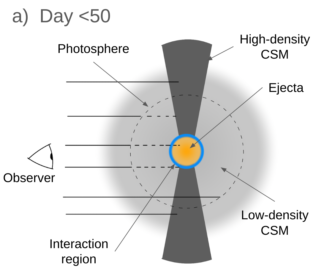
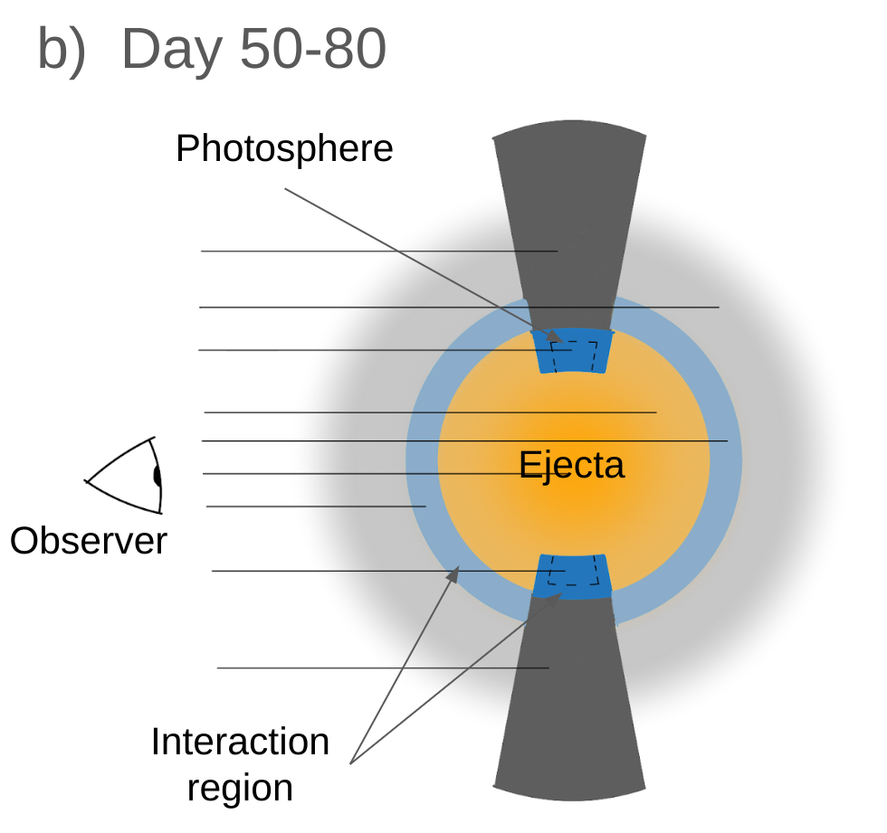
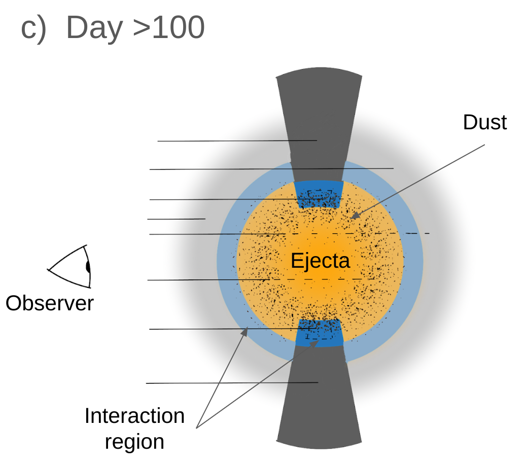
Figure 11: Cartoon diagram representing the evolution of ASASSN-14il through various distinct phases. Representative line-of-sights (LOSs) are shown by solid lines, where dashed lines indicate hindered LOSs. A dense disk-like CSM is located face-on to the observer, and A low-density CSM is present elsewhere. Interaction with dense CSM gives rise to most of the luminosity. At mid-phases, the photosphere recedes from the pre-shock CSM and signatures from the post-shock region and ejecta are visible. At late times the formation of dust obscures the tradition from receding material.

7 Results and Discussion

This paper presents the long-term photometric (up to day 480) and spectroscopic (up to day 327) monitoring campaign of a SN IIn ASASSN-14il. The lightcurves show bumpy behavior at different stages, which can be attributed to ejecta interacting with regions of enhanced CSM density. The multi-band lightcurves also display a plateau-like behavior due to ongoing interaction. A similar plateau is seen in SNe IIn-P (Mauerhan et al., 2013) followed by a steep drop (2-4 mag in optical) from the plateau into a radioactivity-dominated tail. In contrast, some SNe IIn show a plateau followed by a linear decline (Nyholm et al., 2020). However, we can not ascertain the nature of ASASSN-14il in the context of these two classes due to gaps in the observations. ASASSN-14il, with a peak absolute magnitude M_r $\sim-20.3\pm 0.2$ mag, is one of the brightest SN IIn. In UV bands, it is brighter than $-21$ mag, which satisfies the criteria for SLSN category (Gal-Yam, 2012). However, whether such bright interacting transients form a separate population or fall in the tail end of normal SNe IIn is unclear. The color curves are concordant with a typical SN IIn. Overall, it bears a stark resemblance with SN 2015da in terms of the lightcurve and color evolution which indicates similar powering mechanism(s).

Both wind and shell type CSM models in MOSFiT can reproduce the broad lightcurve features of ASASSN-14il. To reproduce the observed luminosities of ASASSN-14il, a high amount of ejecta mass (a few tens to hundred M_⊙) is required to interact with a high-density CSM ($\sim$ 10^-11 g cm^-3). These one-zone models, however, can not reproduce the steep decline of UV lightcurves and the small bump seen in the optical lightcurves around day 90. The assumptions of homologous expansion, constant opacity, and spherical symmetry are simply not representative of the actual explosion scenario. More sophisticated modeling techniques are required to adequately model the lightcurve, which is beyond the scope of this work.

The spectral evolution of ASASSN-14il resembles typical SNe IIn dominated by smooth blue continuum and Balmer lines. The Balmer lines are dominated by Lorentzian wings in the early epochs. The H$\alpha$ line profile evolves to be more complex and multicomponent after day 50. The signs of underlying high-velocity ejecta are visible after this epoch. The emergence of ejecta signatures at the time of peak optical luminosity indicates asymmetries in the explosion/CSM geometry, which is quite common in SNe IIn (Smith, 2017; Bilinski et al., 2024). This is further discussed in subsection 7.2.

After day 123.0, a prominent overall blueshift can be observed in the H$\alpha$ profile, which becomes more pronounced in the final spectra at day 327. The spectra of ASASSN-14il show similarity with SNe 2006gy, 2010jl, and 2015da. The late-time flat-topped profile is reminiscent of SN 2005ip. Also, the late-time blueshift can be explained by dust formation in the post-shock CSM or ejecta (similar to SNe 2005ip, 2010jl, and 2015da; Smith et al., 2009b, 2012, 2023). The case of dust formation and alternative explanation are discussed in subsection 7.4. The evolution of H$\alpha$ to H$\beta$ flux ratio supports the transition scenario from recombination to collisional excitation. The line luminosity of H$\alpha$ shows an increasing trend due to persistent ongoing interaction.

7.1 Narrow lines

ASASSN-14il shows narrow lines throughout its spectral evolution. However, the narrow lines do not show a P-Cygni profile which is expected from a CSM outflow. The lack of a narrow-width P-Cygni feature is very uncommon among SNe IIn. In the case of ASASSN-14il, there could be several reasons for the lack of this feature. First, it could be just due to the spectral resolution of the available spectra. P-Cygni profiles corresponding to outflow velocities of $<100$ km s^-1 would be unresolved in the presented spectra. An unresolved P-Cygni profile will appear redshifted as explained by Smith et al. (2023), and there are indeed some hints of it as the narrow HeI 5876 feature is redshifted from its expected rest wavelength. It is possible that ASASSN-14il is surrounded by an asymmetric CSM structure such that the CSM along the line-of-sight has a relatively lower density (as well as slow-moving) which will give rise to a weaker P-Cygni feature that is hard to resolve under limiting conditions. Secondly, it could be due to the contamination of the narrow lines by the host-galaxy emission.

Additionally, a recent study by Ishii et al. (2024) explores the relations between the line shapes and CSM structure by Monte Carlo radiative transfer codes. They find that a narrow line exhibits a P-Cygni profile only when an eruptive mass-loss event forms the CSM. The CSM structure from a steady mass loss will have a negative velocity gradient after the SN event due to radiative acceleration. Therefore, an H$\alpha$ photon emitted at the deeper CSM layers, traveling outwards, will never be able to undergo another H$\alpha$ transition. Therefore, the CSM residing in the direction of the observer may be created by steady-mass loss (e.g., LBV winds) in the case of ASASSN-14il.

7.2 Asymmetry

In a spherical symmetric model for interacting SNe at early times the continuum photosphere lies in the CSM ahead of the shock. After some time, the photosphere moves into the post-shock CDS, and the uninterrupted ejecta is visible only at late times when the interaction has slowed down enough (Smith, 2017). The line profile of H$\alpha$ earlier spectra (up to day 31) of ASASSN-14il show a symmetric Lorentzian profile expected from the continuum being in the pre-shock CSM. However, the broad component from the SN ejecta is visible as soon as day $50$, along with the intermediate component from the post-shock CDS. The optical luminosity is near-peak at this epoch, indicating the presence of strong CSM interaction. This is not explained from a spherically symmetric CSM geometry. Instead, the emergence of broad ejecta suggests significantly lower CSM along the LOS compared to the CSM needed to sustain the peak luminosity. This can be explained by an asymmetric CSM configuration such that dense CSM, at angles alternate to the LOS, giving rise to the majority of the observed luminosity. Such a configuration is not uncommon in SNe IIn. SNe 2010jl, 2012ab, and 2015da all reveal the underlying ejecta earlier than expected from a spherical CSM distribution and are suggested to feature a disk-like/torus-like CSM geometry (Katsuda et al., 2016; Bilinski et al., 2020; Gangopadhyay et al., 2020; Smith et al., 2023).

A recent spectropolarimetry study of SNe IIn (including ASASSN-14il) by Bilinski et al. (2024) reveals a significant amount of polarization in the majority of events in their sample, indicating asymmetries in the CSM. They study ASASSN-14il at 3 epochs (day 31, 63, 119 from the explosion date estimated in this work). There is a change in continuum polarization going from day 31 to 63, which coincides with the transition of the continuum photosphere from the pre-shock CSM to CDS/ejecta. The continuum polarization of ASASSN-14il is one of the lowest (along with SN 2014ab) in the sample. Additionally, there is no significant line depolarization noticed in ASASSN-14il. This polarization doesn’t necessarily eliminate the possibility of asymmetric CSM; instead, they can be explained in a complimentary manner. A disk-like CSM viewed from the polar region will have a face-on symmetry for the continuum photosphere and, therefore, low-polarization (Bilinski et al., 2020).

7.3 Mass-loss Rate

The intermediate-width component seen throughout the evolution of ASASSN-14il indicates the persistent ejecta-CSM interaction, as also observed in the case of SN 2012ab (Gangopadhyay et al., 2020). Assuming that the luminosity of the ejecta-CSM interaction is fed by energy at the shock front, the progenitor mass loss rate $\dot{M}$ can be calculated using the relation of Chugai & Danziger (1994):

$$\dot{M}=\frac{2L}{\epsilon}\frac{v_{w}}{v_{SN}^{3}}$$ (1)

where $\epsilon$ ($<1$) is the efficiency of conversion of the shock’s kinetic energy into optical radiation (an uncertain quantity), $v_{w}$ is the velocity of the pre-explosion stellar wind, $v_{\mathrm{SN}}$ is the velocity of the post-shock shell, and $L$ is the bolometric luminosity of ASASSN-14il. We assume typical unshocked wind velocity observed for LBV winds $v_{w}$$\sim$100 km sec^-1. The shock velocity is inferred from the intermediate width component after the emission lines are no longer dominated by electron scattering (day $>=$ 50). We take the shock velocity to be 1750 km s^-1, similar to the value used by Dickinson (2021). Using the bolometric luminosity at day $\sim 50$ (L=4.7 x 10⁴³ erg sec^-1) and assuming 50$\%$ conversion efficiency with $\epsilon$=0.5, the estimated mass-loss rate for ASASSN-14il is 5.6 M_⊙ yr^-1. However, we find that the estimated mass-loss rate is 1.0 M_⊙ yr^-1 for only the integrated observed luminosity with no bolometric corrections. Dickinson (2021) found the mass-loss rate to be 1 M_⊙ yr^-1 following similar analysis based on the V-band luminosity. These values are also comparable to the mass-loss value for the csm_s2 model derived from lightcurve fitting.

These values are comparable, albeit slightly higher, than the estimates for SN 2015da (Smith et al., 2023) at similar epochs. This can be attributed to higher bolometric luminosity and slower shock speed in ASASSN-14il. The estimated value of mass-loss rate is much higher than the typical LBV winds (Smith, 2014) and higher than the values often attributed to some SNe IIn, which are of the order of 0.1 M_⊙ yr^-1 as observed in some giant eruptions of LBVs (Chugai et al., 2004; Kiewe et al., 2012). These values are also much higher than those of normal-luminosity SNe IIn like SN 2005ip ($2-4\times 10^{-4}$ M_⊙ yr^-1; Smith et al., 2009b). It is also much larger than the typical values of RSG and yellow hypergiants ($10^{-4}-10^{-3}$ M_⊙ yr^-1; Smith, 2014), and quiescent winds of LBV (10${}^{-5}-10^{-4}$ M_⊙ yr^-1, Vink, 2018). The obtained mass-loss rate in ASASSN-14il indicates the probable progenitor to be an LBV star that underwent an eruptive phase. The CSM may be the result of interaction with a binary companion, which in would explain the expected asymmetry in the geometry.

7.4 A case for Dust Formation

The H$\alpha$ profile of ASASSN-14il shows a deficit in the flux of the redside wing. This deficit is clearly visible as an overall blueshift of the line after day 100 and increases with time. At day 327, even a combination of blueshifted Gaussian components can not appropriately reproduce the H$\alpha$ line profile. At this epoch, the line profile can be best described as missing flux from the redside wing and near rest velocity. The flux deficit phenomenon is wavelength dependent as well, affecting the shorter wavelength H$\beta$ more severely compared to H$\alpha$.

An overall blueshift could be caused by many reasons, such as radiative acceleration, lopsided SN explosion or asymmetric CSM, obscuration of the receding material by the continuum photosphere, and dust formation. However, except for dust formation, none of the other mechanisms can explain the observed time dependence and wavelength dependence.

In the case of a blueshift caused by the radiative acceleration of the CSM, the blueshift should decrease as the luminosity drops, and we expect no significant wavelength dependence for this case. Additionally, in the case of a blueshift caused by the radiative acceleration scenario, the original narrow line photon source should be blueshifted as well, which is not the case for ASASSN-14il (Dessart et al., 2015). Similarly, in the case of obscuration by the continuum photosphere, the expected blueshift will be strongest in early times and decrease later on as the continuum optical depth drops. For a lopsided explosion/CSM any blueshift present should be present from early times as well, remaining consistent throughout the evolution. Thus none of these scenarios are consistent with the observed evolution of ASASSN-14il.

However, all these requirements are readily explained by a scenario where new dust grains form in the ejecta or the post-shock CSM. The dust formation will increase at late times as the ejecta and the post-shock CSM cool down, explaining the time evolution of the observed deficit of flux in the side wing of H$\alpha$. Also, the wavelength dependence of the flux deficit is a natural consequence of the extinction from dust affecting shorter wavelengths more prominently. Dust formation has other signatures, such as an increase in the NIR flux and an increased rate of fading the optical flux. However, due to data gaps between days 120–250 and the lack of late-time NIR data, we are unable to comment on it. Dust formation is very common in SLSNe IIn as seen in the case of SNe 2006tf (Smith et al., 2008), 2010jl Smith et al. (2012); Maeda et al. (2013); Gall et al. (2014), 2015da Smith et al. (2023), ASASSN-15ua Dickinson et al. (2023), and 2017hcc Smith & Andrews (2020), so expecting dust formation in ASASSN-14il would not be unreasonable.

7.5 Physical Scenario

Figure 11 describes a physical scenario that, although not unique, explains the observables of ASASSN-14il through various stages of its evolution. In this scenario, the ejecta from the SN explosion interacts with a disk-like CSM. The viewing angle of the observer is such that the CSM disk is face-on to the observer. This configuration is surrounded by distant CSM that may result from steady mass loss from the progenitor.

Figure 11a describes a scenario where the photosphere lies in the pre-shock CSM surrounding the interaction region. The line profiles are dominated by narrow lines and Lorentzian wings resulting from electron scattering in the ionized CSM. The signatures from the SN ejecta are masked by the interaction region. This figure explains the observed line profile in ASASSN-14il at early phases ($<$ day 50).

Between day 50–80, the photosphere recedes into the interaction region. Due to the asymmetric CSM geometry, both uninterrupted SN ejecta and post-shock region are visible simultaneously (Figure 11b). The line profiles see contributions from the SN ejecta, shock region, and distant uninterrupted CSM, which manifests as broad, intermediate, and narrow-width Gaussian components, respectively.

Figure 11c depicts the evolution of ASASSN-14il post day 80. The contributions from the distant CSM, post-shock region, and the ejecta are still seen. Dust formation is seen in the post-shock gas, an efficient location for dust formation in SNe IIn. This dust preferentially obscures the receding SN ejecta and shock, causing a deficit in the redside wing of line profiles. This effect manifests as an overall blueshift of the broad component. Such blueshift is observed in the late time ($>$ day 100) H$\alpha$ profile of ASASSN-14il as well as many other SNe IIn (e.g. SNe 2005ip, 20006tf, 2010jl, ASASSN-15ua, 2015da).

Similar explosion/CSM geometry have been proposed for SNe 2010jl, 2014ab, 2015da, and 2017hcc (Smith et al., 2011; Bilinski et al., 2020; Smith et al., 2023; Smith & Andrews, 2020) with different viewing angles. However, the viewing angle in SN 2014ab and ASASSN-14il are proposed to be similar, which is further emphasized by both having remarkably low polarization (Bilinski et al., 2024).

8 Summary

1. ASASSN-14il was observed with an extensive follow-up campaign spanning $\sim 480$ days in photometric and $\sim 327$ days in spectroscopy observations.

2. ASASSN-14il is a very luminous SN IIn showing long-term interaction signatures and a plateau in the optical light curves around the maximum. It peaks at $\sim-20.3$ mag in r-band ($<-21$ mag in UV bands), comparable to SLSNe 2006tf, 2010jl, ASASSN-15ua. The lightcurve shape is very similar to SN 2015da, but the late time (after $\sim 250$ days) decline rate of $\sim$0.01 mag/day in optical bands is faster than SN 2015da but comparable to SNe 2006tf, 2010jl, ASASSN-15ua. The slow reward evolution of the intrinsic B-V resembles the typical SNe IIn.

3. The multi-band lightcurve modeling of ASASSN-14il indicates a CSM-driven explosion. Both wind/shell CSM model generates our observed lightcurves with a CSM mass between 4.7–9.1 M_⊙ and the CSM shell/wind being expelled about 1-5 years before the explosion.

4. Spectroscopically, ASASSN-14il shows long-term predominant interaction signatures with narrow H and He lines on top of otherwise featureless spectra similar to other SLSNe IIn 2006gy, 2010jl, and 2015da.

5. The H$\alpha$ profile of ASASSN-14il can be described by the following components- (i) An unresolved component from the pre-shock ionized CSM that stays consistent throughout the evolution, (ii) An intermediate width component initially dominated by Lorentzian electron-scattering wings but later (day $>50$) show Gaussian profile (FWHM $\sim$ 1750 km s^-1) representative of the post-shock region. (iii) A broad Gaussian emission component (FWHM $\sim$ 7000 km s^-1) representative of the uninterrupted ejecta, which becomes visible (day $>50$).

6. The emergence of the ejecta component when the lightcurves are near peak luminosity indicates asymmetry in the CSM structure.

7. The blueshift of H$\alpha$ profile at late phases (day $>100$) indicates dust formation in the post-shock CSM/ejecta.

8. The mass-loss rate of 2-7 M${}_{\odot}\mathrm{yr}^{-1}$ indicates that the progenitor star is most likely an LBV that underwent an eruptive phase.

Appendix A Observation log

Table 7: Log of photomteric observations of ASASSN-14il obtained from LCOGT network of telescopes.

Date	Phase	B	V	g	r	i	telescope
(yyyy-mm-dd)	(d)	(mag)	(mag)	(mag)	(mag)	(mag)
2014-10-03	7.8	$16.15\pm 0.03$	$16.25\pm 0.04$	$15.97\pm 0.02$	$16.10\pm 0.04$	$16.14\pm 0.01$	1m0-12
2014-10-05	9.5	$16.15\pm 0.02$	$16.07\pm 0.01$	$15.87\pm 0.04$	$15.91\pm 0.02$	$16.07\pm 0.01$	1m0-11
2014-10-07	11.3	$16.10\pm 0.08$	$15.71\pm 0.06$	$15.75\pm 0.05$	$15.84\pm 0.11$	-	1m0-08
2014-10-09	13.3	-	$15.58\pm 0.16$	$15.57\pm 0.05$	$15.54\pm 0.15$	$15.70\pm 0.20$	1m0-08
2014-10-09	13.7	$15.87\pm 0.02$	$15.74\pm 0.03$	$15.50\pm 0.02$	$15.52\pm 0.04$	$15.65\pm 0.05$	1m0-11
2014-10-11	15.5	$15.84\pm 0.06$	$15.63\pm 0.01$	$15.42\pm 0.01$	$15.52\pm 0.03$	$15.68\pm 0.05$	1m0-03
2014-10-13	17.9	$15.76\pm 0.04$	$15.55\pm 0.01$	$15.44\pm 0.01$	$15.45\pm 0.02$	$15.53\pm 0.01$	1m0-10
2014-10-15	19.3	$15.74\pm 0.05$	$15.57\pm 0.03$	$15.37\pm 0.02$	$15.42\pm 0.02$	$15.56\pm 0.02$	1m0-08
2014-10-17	22.0	$15.74\pm 0.03$	$15.44\pm 0.02$	$15.39\pm 0.01$	$15.37\pm 0.04$	$15.44\pm 0.04$	1m0-13
2014-10-18	22.2	$15.63\pm 0.01$	$15.38\pm 0.03$	$15.23\pm 0.01$	$15.33\pm 0.01$	$15.39\pm 0.05$	1m0-08
2014-10-19	23.9	$15.68\pm 0.02$	-	-	-	-	1m0-12
2014-10-20	24.5	$15.54\pm 0.06$	$15.40\pm 0.04$	$15.27\pm 0.02$	$15.22\pm 0.02$	$15.28\pm 0.03$	1m0-03
2014-10-20	24.4	$15.54\pm 0.02$	$15.30\pm 0.03$	$15.21\pm 0.01$	$15.21\pm 0.01$	$15.27\pm 0.02$	1m0-11
2014-10-21	25.9	$15.70\pm 0.02$	$15.37\pm 0.02$	$15.30\pm 0.01$	$15.25\pm 0.03$	$15.31\pm 0.02$	1m0-10
2014-10-22	26.5	$15.59\pm 0.02$	$15.30\pm 0.04$	$15.18\pm 0.03$	-	$15.31\pm 0.10$	1m0-03
2014-10-26	30.5	$15.65\pm 0.02$	$15.32\pm 0.07$	$15.22\pm 0.02$	$15.13\pm 0.02$	$15.17\pm 0.05$	1m0-11
2014-10-29	34.0	-	$15.33\pm 0.02$	$15.24\pm 0.01$	$15.14\pm 0.03$	$15.19\pm 0.05$	1m0-12
2014-11-02	37.7	-	$15.32\pm 0.09$	-	-	-	1m0-03
2014-11-06	41.4	-	$15.15\pm 0.03$	$15.23\pm 0.02$	$15.04\pm 0.03$	-	1m0-11
2014-11-10	45.2	-	$15.20\pm 0.04$	$15.32\pm 0.04$	$15.10\pm 0.04$	$15.09\pm 0.03$	1m0-08
2014-11-13	49.0	$15.73\pm 0.03$	$15.22\pm 0.02$	$15.23\pm 0.03$	$15.06\pm 0.03$	$15.06\pm 0.02$	1m0-12
2014-11-17	52.8	$15.62\pm 0.02$	$15.26\pm 0.02$	$15.34\pm 0.01$	$15.11\pm 0.04$	$15.02\pm 0.03$	1m0-12
2014-11-21	56.6	-	$15.26\pm 0.04$	$15.27\pm 0.02$	$15.04\pm 0.03$	$14.98\pm 0.03$	1m0-03
2014-11-26	61.9	$15.78\pm 0.02$	-	$15.23\pm 0.02$	$15.04\pm 0.02$	$14.97\pm 0.02$	1m0-10
2014-11-26	62.0	-	-	$15.31\pm 0.03$	$15.05\pm 0.01$	$14.97\pm 0.04$	1m0-13
2014-11-27	62.2	$15.76\pm 0.03$	$15.29\pm 0.04$	$15.31\pm 0.01$	$15.08\pm 0.02$	$15.03\pm 0.02$	1m0-05
2014-11-27	62.0	$15.67\pm 0.01$	$15.18\pm 0.03$	$15.26\pm 0.01$	$15.04\pm 0.04$	$15.00\pm 0.04$	1m0-08
2014-11-28	63.8	$15.89\pm 0.04$	$15.30\pm 0.02$	$15.39\pm 0.01$	$15.08\pm 0.03$	$14.98\pm 0.05$	1m0-12
2014-12-02	67.4	-	-	-	$15.09\pm 0.05$	$15.10\pm 0.04$	1m0-03
2014-12-04	69.8	$15.92\pm 0.02$	$15.27\pm 0.03$	$15.43\pm 0.02$	$15.06\pm 0.02$	$15.03\pm 0.04$	1m0-10
2014-12-04	69.9	$15.81\pm 0.01$	$15.27\pm 0.02$	$15.38\pm 0.01$	$15.07\pm 0.01$	$14.92\pm 0.04$	1m0-12
2014-12-09	74.2	$15.84\pm 0.02$	$15.23\pm 0.03$	$15.32\pm 0.02$	$14.99\pm 0.03$	$15.02\pm 0.01$	1m0-05
2014-12-12	77.8	$15.93\pm 0.03$	$15.17\pm 0.03$	$15.48\pm 0.02$	-	-	1m0-12
2014-12-12	77.9	$15.88\pm 0.03$	$15.15\pm 0.06$	$15.48\pm 0.05$	$15.05\pm 0.03$	$14.92\pm 0.01$	1m0-13
2014-12-16	81.8	$15.97\pm 0.03$	$15.28\pm 0.02$	$15.34\pm 0.03$	$15.05\pm 0.02$	$14.89\pm 0.03$	1m0-12
2014-12-20	85.8	$15.91\pm 0.04$	$15.27\pm 0.01$	$15.41\pm 0.02$	$15.00\pm 0.05$	$14.87\pm 0.03$	1m0-12
2014-12-24	89.5	$15.72\pm 0.02$	$15.10\pm 0.02$	$15.22\pm 0.02$	$14.89\pm 0.02$	$14.83\pm 0.04$	1m0-03
2014-12-29	94.5	$15.82\pm 0.01$	$15.23\pm 0.10$	$15.41\pm 0.02$	-	-	1m0-11
2015-01-02	98.5	-	-	-	$14.83\pm 0.03$	$14.78\pm 0.03$	1m0-11
2015-01-06	102.4	$15.87\pm 0.03$	$15.27\pm 0.01$	$15.32\pm 0.01$	$14.93\pm 0.02$	$14.79\pm 0.05$	1m0-03
2015-01-11	107.8	$16.07\pm 0.01$	$15.31\pm 0.02$	$15.54\pm 0.02$	$15.04\pm 0.01$	$14.89\pm 0.02$	1m0-13
2015-01-15	111.8	$16.19\pm 0.04$	$15.33\pm 0.01$	$15.52\pm 0.02$	-	-	1m0-13
2015-01-16	112.1	$15.98\pm 0.02$	$15.33\pm 0.03$	$15.48\pm 0.01$	$15.05\pm 0.02$	$14.96\pm 0.02$	1m0-05
2015-01-19	115.8	$16.02\pm 0.02$	$15.37\pm 0.04$	$15.51\pm 0.02$	$15.04\pm 0.02$	$14.89\pm 0.05$	1m0-10
2015-01-28	124.0	$16.24\pm 0.05$	$15.58\pm 0.04$	$15.63\pm 0.02$	$15.14\pm 0.01$	$15.08\pm 0.02$	1m0-05
2015-02-06	133.4	$16.09\pm 0.08$	$15.37\pm 0.01$	$15.59\pm 0.01$	$15.11\pm 0.02$	$14.99\pm 0.06$	1m0-03
2015-06-19	266.2	-	$17.09\pm 0.08$	$17.33\pm 0.02$	$16.53\pm 0.02$	$16.44\pm 0.08$	1m0-12
2015-06-24	271.4	-	-	$17.28\pm 0.02$	$16.85\pm 0.09$	$16.77\pm 0.02$	1m0-05
2015-06-28	275.8	$17.97\pm 0.03$	$16.97\pm 0.03$	$17.44\pm 0.03$	$16.59\pm 0.04$	-	1m0-11
2015-07-02	279.2	$17.71\pm 0.15$	$17.22\pm 0.04$	$17.45\pm 0.07$	$16.71\pm 0.01$	$16.92\pm 0.02$	1m0-12
2015-07-02	279.2	$17.79\pm 0.17$	$17.26\pm 0.04$	$17.24\pm 0.09$	$16.61\pm 0.03$	$16.76\pm 0.13$	1m0-13
2015-07-06	283.0	$17.49\pm 0.20$	-	$17.77\pm 0.11$	$16.50\pm 0.19$	$16.76\pm 0.03$	1m0-12
2015-07-09	286.7	-	$17.40\pm 0.08$	-	$16.53\pm 0.05$	$16.76\pm 0.22$	1m0-11
2015-07-14	291.4	$18.12\pm 0.05$	$17.42\pm 0.09$	$17.52\pm 0.03$	$16.75\pm 0.04$	$16.86\pm 0.02$	1m0-05
2015-07-18	295.4	$18.38\pm 0.22$	$17.37\pm 0.04$	$17.38\pm 0.08$	$16.57\pm 0.06$	$16.92\pm 0.08$	1m0-08
2015-07-23	300.4	$18.38\pm 0.16$	$17.44\pm 0.06$	$17.55\pm 0.04$	$16.63\pm 0.06$	$16.96\pm 0.01$	1m0-05
2015-07-26	303.7	-	$17.31\pm 0.02$	$17.60\pm 0.07$	$16.63\pm 0.01$	$16.84\pm 0.04$	1m0-03
2015-07-30	307.4	$18.41\pm 0.05$	$17.53\pm 0.13$	-	$16.91\pm 0.02$	$17.04\pm 0.09$	1m0-05
2015-08-25	333.4	-	$17.82\pm 0.04$	$17.81\pm 0.03$	$16.99\pm 0.04$	$17.11\pm 0.09$	1m0-08
2015-09-04	343.9	$18.60\pm 0.13$	$17.60\pm 0.12$	$17.89\pm 0.02$	$17.18\pm 0.03$	$17.26\pm 0.08$	1m0-10
2015-09-05	344.1	$18.45\pm 0.05$	$17.92\pm 0.03$	-	-	-	1m0-10
2015-09-05	344.1	-	$17.68\pm 0.30$	$17.96\pm 0.12$	$17.18\pm 0.07$	$17.63\pm 0.04$	1m0-12
2015-09-05	344.0	-	$17.90\pm 0.07$	$18.05\pm 0.04$	$17.04\pm 0.09$	-	1m0-13
2015-09-15	354.8	$18.65\pm 0.30$	$17.76\pm 0.13$	$17.97\pm 0.04$	-	$17.42\pm 0.13$	1m0-12
2015-09-18	357.3	$18.89\pm 0.05$	$18.26\pm 0.16$	$18.13\pm 0.09$	$17.27\pm 0.01$	$17.56\pm 0.05$	1m0-05
2015-09-28	368.0	-	-	$18.16\pm 0.08$	-	-	1m0-10
2015-09-29	368.0	-	-	-	$17.28\pm 0.11$	-	1m0-10
2015-10-14	383.2	-	$18.50\pm 0.06$	$18.30\pm 0.14$	$17.50\pm 0.02$	$18.02\pm 0.12$	1m0-08
2015-10-27	396.2	-	-	$18.53\pm 0.21$	$17.64\pm 0.11$	-	1m0-05
2015-11-06	406.9	$19.44\pm 0.12$	-	$18.87\pm 0.03$	$18.05\pm 0.01$	$17.80\pm 0.19$	1m0-10
2015-11-17	417.6	$19.49\pm 0.40$	$18.80\pm 0.32$	$19.18\pm 0.12$	-	$18.06\pm 0.11$	1m0-03
2015-11-19	419.6	-	$18.75\pm 0.03$	-	-	$18.09\pm 0.23$	1m0-03
2015-11-21	421.2	-	-	$18.88\pm 0.15$	$18.01\pm 0.19$	-	1m0-05
2015-12-14	444.1	$20.40\pm 0.23$	-	$19.15\pm 0.11$	-	$18.57\pm 0.09$	1m0-05
2015-12-25	455.1	-	-	-	$18.72\pm 0.29$	$18.47\pm 0.17$	1m0-05
2016-01-07	468.4	$20.46\pm 0.18$	-	-	$18.78\pm 0.18$	-	1m0-03
2016-01-07	468.1	-	-	$19.59\pm 0.17$	$18.40\pm 0.08$	-	1m0-05
2016-01-07	468.8	-	-	-	$18.66\pm 0.23$	-	1m0-10
2016-01-19	480.1	-	-	-	$18.74\pm 0.08$	-	1m0-05

Table 8: Log of Swift UV and optical photometric observations of ASASSN-14il.

Phase	MJD	UVW1	UVW2	UVM2	U	B	V	Instrument
(d)		(mag)	(mag)	(mag)	(mag)	(mag)	(mag)
7.90	56933.90	$14.70\pm 0.08$	$14.72\pm 0.07$	$14.69\pm 0.08$	$14.81\pm 0.07$	$16.08\pm 0.11$	$16.08\pm 0.16$	UVOT
9.99	56935.99	$14.46\pm 0.07$	$14.57\pm 0.07$	$14.45\pm 0.06$	$14.68\pm 0.07$	$16.03\pm 0.10$	$15.88\pm 0.14$	UVOT
11.84	56937.84	$14.41\pm 0.06$	$14.54\pm 0.06$	$14.42\pm 0.06$	$14.54\pm 0.06$	$15.83\pm 0.09$	$15.77\pm 0.11$	UVOT
13.83	56939.83	$14.36\pm 0.07$	$14.50\pm 0.07$	$14.39\pm 0.06$	$14.44\pm 0.06$	$15.67\pm 0.09$	$15.64\pm 0.12$	UVOT
15.43	56941.43	$14.29\pm 0.06$	$14.49\pm 0.07$	$14.37\pm 0.06$	$14.40\pm 0.06$	$15.55\pm 0.08$	$15.55\pm 0.11$	UVOT
16.88	56942.88	$14.29\pm 0.06$	$14.58\pm 0.07$	-	$14.37\pm 0.06$	$15.64\pm 0.09$	-	UVOT
16.94	56942.94	-	$14.58\pm 0.07$	$14.53\pm 0.08$	-	-	$15.66\pm 0.14$	UVOT
17.83	56943.83	$14.35\pm 0.06$	$14.61\pm 0.07$	$14.50\pm 0.07$	$14.35\pm 0.06$	$15.57\pm 0.08$	$15.68\pm 0.12$	UVOT
18.69	56944.69	-	$14.63\pm 0.07$	-	$14.32\pm 0.06$	-	-	UVOT
18.87	56944.87	$14.28\pm 0.06$	$14.59\pm 0.07$	$14.55\pm 0.07$	$14.33\pm 0.06$	$15.60\pm 0.09$	$15.50\pm 0.11$	UVOT
21.37	56947.37	$14.39\pm 0.06$	$14.66\pm 0.07$	$14.57\pm 0.07$	$14.34\pm 0.06$	$15.55\pm 0.09$	$15.25\pm 0.10$	UVOT
23.25	56949.25	$14.38\pm 0.06$	$14.70\pm 0.07$	$14.59\pm 0.07$	$14.33\pm 0.06$	$15.40\pm 0.08$	$15.27\pm 0.10$	UVOT
25.37	56951.37	-	-	$14.58\pm 0.08$	-	-	$15.25\pm 0.12$	UVOT
25.67	56951.67	$14.45\pm 0.07$	$14.79\pm 0.08$	-	$14.31\pm 0.06$	$15.42\pm 0.08$	-	UVOT
29.42	56955.42	$14.55\pm 0.07$	$14.92\pm 0.08$	$14.78\pm 0.08$	$14.38\pm 0.06$	$15.40\pm 0.08$	$15.25\pm 0.10$	UVOT
31.34	56957.34	$14.63\pm 0.07$	$15.02\pm 0.08$	$14.93\pm 0.08$	$14.46\pm 0.06$	$15.34\pm 0.07$	$15.23\pm 0.10$	UVOT
33.47	56959.47	$14.77\pm 0.08$	-	-	-	-	-	UVOT
35.92	56961.92	$14.88\pm 0.08$	$15.36\pm 0.10$	$15.18\pm 0.09$	$14.52\pm 0.06$	$15.43\pm 0.08$	$15.21\pm 0.09$	UVOT
37.85	56963.85	$15.00\pm 0.08$	$15.41\pm 0.10$	$15.27\pm 0.09$	$14.60\pm 0.06$	$15.41\pm 0.08$	$15.23\pm 0.09$	UVOT
40.78	56966.78	$15.13\pm 0.09$	$15.56\pm 0.11$	$15.40\pm 0.09$	$14.63\pm 0.07$	$15.40\pm 0.08$	$15.23\pm 0.09$	UVOT
42.21	56968.21	$15.14\pm 0.09$	-	-	$14.64\pm 0.07$	$15.47\pm 0.08$	-	UVOT
46.23	56972.23	$15.42\pm 0.10$	$16.02\pm 0.14$	$15.79\pm 0.11$	$14.78\pm 0.07$	$15.46\pm 0.08$	$15.15\pm 0.09$	UVOT
48.31	56974.31	$15.45\pm 0.10$	$16.05\pm 0.14$	$15.87\pm 0.11$	$14.85\pm 0.07$	$15.57\pm 0.08$	$15.18\pm 0.09$	UVOT

Table 9: Log of spectroscopic observations of ASASSN-14il.

Date	MJD	phase	Telescope	Range	Resolution
(yy-mm-dd)	(day)		(Å)	($\lambda/\Delta\lambda$)
2014-10-03	56933.55	7.6	ANU+WiFeS	3050 - 11000	3000
2014-10-03	56933.73	7.7	LCO+FLOYDS	3200 - 10000	400 - 700
2014-10-05	56935.63	9.6	LCO+FLOYDS	3200 - 10000	400 - 700
2014-10-07	56937.71	11.7	LCO+FLOYDS	3200 - 10000	400 - 700
2014-10-09	56939.50	13.5	ANU+WiFeS	3050 - 11000	3000
2014-10-10	56940.47	14.5	LCO+FLOYDS	3200 - 10000	400 - 700
2014-10-13	56943.64	17.6	LCO+FLOYDS	3200 - 10000	400 - 700
2014-10-14	56944.06	18.1	ESO-NTT + SOFI	9000 - 25000	600 - 2200
2014-10-18	56948.56	22.6	ANU+WiFeS	3050 - 11000	3000
2014-10-18	56948.67	22.7	LCO+FLOYDS	3200 - 10000	400 - 700
2014-10-22	56952.02	26.0	ESO-NTT + EFOSC	3050 - 11000	-
2014-10-22	56952.47	26.5	LCO+FLOYDS	3200 - 10000	400 - 700
2014-10-24	56954.21	28.2	ESO-NTT + SOFI	9000 - 25000	600 - 2200
2014-10-27	56957.47	31.5	ANU+WiFeS	3050 - 11000	3000
2014-11-14	56975.16	49.2	ESO-NTT + EFOSC	3050 - 11000	-
2014-11-15	56976.19	50.2	ESO-NTT + SOFI	9000 - 25000	600 - 2200
2014-12-16	57007.51	81.5	LCO+FLOYDS	3200 - 10000	400 - 700
2014-12-22	57013.08	87.1	ESO-NTT + SOFI	9000 - 25000	600 - 2200
2015-01-13	57035.06	109.1	ESO-NTT + EFOSC	3050 - 11000	-
2015-01-20	57042.06	116.1	ESO-NTT + SOFI	9000 - 25000	600 - 2200
2015-01-27	57049.04	123.0	ESO-NTT + EFOSC	3050 - 11000	-
2015-08-19	57253.26	327.3	ESO-NTT + EFOSC	3050 - 11000	-

Appendix B MOSFiT Corner Plot

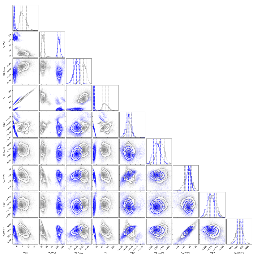
Figure 12: Corner plot showing the best fit parameters of the csm wind (blue) and csm shell (gray) models for ASASSN-14il.

References

- Agnoletto (2009) Agnoletto, I. 2009, in American Institute of Physics Conference Series, Vol. 1111, American Institute of Physics Conference Series, ed. G. Giobbi, A. Tornambe, G. Raimondo, M. Limongi, L. A. Antonelli, N. Menci, & E. Brocato, 430–434, doi: 10.1063/1.3141587
- Bak Nielsen et al. (2018) Bak Nielsen, A.-S., Hjorth, J., & Gall, C. 2018, A&A, 611, A67, doi: 10.1051/0004-6361/201629904
- Balberg & Loeb (2011) Balberg, S., & Loeb, A. 2011, MNRAS, 414, 1715, doi: 10.1111/j.1365-2966.2011.18505.x
- Becker (2015) Becker, A. 2015, HOTPANTS: High Order Transform of PSF ANd Template Subtraction, Astrophysics Source Code Library, record ascl:1504.004. http://ascl.net/1504.004
- Benetti et al. (2006) Benetti, S., Cappellaro, E., Turatto, M., et al. 2006, ApJ, 653, L129, doi: 10.1086/510667
- Bilinski et al. (2024) Bilinski, C., Smith, N., Williams, G. G., et al. 2024, MNRAS, 529, 1104, doi: 10.1093/mnras/stae380
- Bilinski et al. (2020) —. 2020, MNRAS, 498, 3835, doi: 10.1093/mnras/staa2617
- Breeveld et al. (2011) Breeveld, A. A., Landsman, W., Holland, S. T., et al. 2011, in American Institute of Physics Conference Series, Vol. 1358, Gamma Ray Bursts 2010, ed. J. E. McEnery, J. L. Racusin, & N. Gehrels, 373–376, doi: 10.1063/1.3621807
- Brimacombe et al. (2014) Brimacombe, J., Holoien, T. W. S., Stanek, K. Z., et al. 2014, The Astronomer’s Telegram, 6525, 1
- Brown et al. (2014) Brown, P. J., Breeveld, A. A., Holland, S., Kuin, P., & Pritchard, T. 2014, Ap&SS, 354, 89, doi: 10.1007/s10509-014-2059-8
- Brown et al. (2009) Brown, P. J., Holland, S. T., Immler, S., et al. 2009, AJ, 137, 4517, doi: 10.1088/0004-6256/137/5/4517
- Chatzopoulos et al. (2012) Chatzopoulos, E., Wheeler, J. C., & Vinko, J. 2012, ApJ, 746, 121, doi: 10.1088/0004-637X/746/2/121
- Chatzopoulos et al. (2013) Chatzopoulos, E., Wheeler, J. C., Vinko, J., Horvath, Z. L., & Nagy, A. 2013, ApJ, 773, 76, doi: 10.1088/0004-637X/773/1/76
- Chevalier (1982) Chevalier, R. A. 1982, ApJ, 258, 790, doi: 10.1086/160126
- Chevalier (1998) —. 1998, ApJ, 499, 810, doi: 10.1086/305676
- Chevalier & Fransson (1994) Chevalier, R. A., & Fransson, C. 1994, ApJ, 420, 268, doi: 10.1086/173557
- Childress et al. (2014) Childress, M., Scalzo, R., Yuan, F., et al. 2014, The Astronomer’s Telegram, 6536, 1
- Childress et al. (2016) Childress, M. J., Tucker, B. E., Yuan, F., et al. 2016, PASA, 33, e055, doi: 10.1017/pasa.2016.47
- Chugai (2001) Chugai, N. N. 2001, MNRAS, 326, 1448, doi: 10.1111/j.1365-2966.2001.04717.x
- Chugai & Danziger (1994) Chugai, N. N., & Danziger, I. J. 1994, MNRAS, 268, 173, doi: 10.1093/mnras/268.1.173
- Chugai et al. (2004) Chugai, N. N., Blinnikov, S. I., Cumming, R. J., et al. 2004, MNRAS, 352, 1213, doi: 10.1111/j.1365-2966.2004.08011.x
- Dessart et al. (2015) Dessart, L., Audit, E., & Hillier, D. J. 2015, MNRAS, 449, 4304, doi: 10.1093/mnras/stv609
- Dessart et al. (2009) Dessart, L., Hillier, D. J., Gezari, S., Basa, S., & Matheson, T. 2009, MNRAS, 394, 21, doi: 10.1111/j.1365-2966.2008.14042.x
- Di Carlo et al. (2002) Di Carlo, E., Massi, F., Valentini, G., et al. 2002, ApJ, 573, 144, doi: 10.1086/340496
- Dickinson et al. (2023) Dickinson, D., Smith, N., Andrews, J. E., et al. 2023, arXiv e-prints, arXiv:2302.04958, doi: 10.48550/arXiv.2302.04958
- Dickinson (2021) Dickinson, D. A. 2021, AN OPTICAL STUDY OF THE SUPERLUMINOUS TYPE IIN SUPERNOVA ASASSN-14IL. http://hdl.handle.net/10150/666597
- Filippenko (1997) Filippenko, A. V. 1997, ARA&A, 35, 309, doi: 10.1146/annurev.astro.35.1.309
- Fox et al. (2009) Fox, O., Skrutskie, M. F., Chevalier, R. A., et al. 2009, ApJ, 691, 650, doi: 10.1088/0004-637X/691/1/650
- Fox et al. (2015) Fox, O. D., Silverman, J. M., Filippenko, A. V., et al. 2015, MNRAS, 447, 772, doi: 10.1093/mnras/stu2435
- Fransson et al. (2002) Fransson, C., Chevalier, R. A., Filippenko, A. V., et al. 2002, ApJ, 572, 350, doi: 10.1086/340295
- Fransson et al. (2014) Fransson, C., Ergon, M., Challis, P. J., et al. 2014, ApJ, 797, 118, doi: 10.1088/0004-637X/797/2/118
- Gal-Yam (2012) Gal-Yam, A. 2012, Science, 337, 927, doi: 10.1126/science.1203601
- Gal-Yam (2019) —. 2019, ARA&A, 57, 305, doi: 10.1146/annurev-astro-081817-051819
- Gal-Yam & Leonard (2009) Gal-Yam, A., & Leonard, D. C. 2009, Nature, 458, 865, doi: 10.1038/nature07934
- Gall et al. (2014) Gall, C., Hjorth, J., Watson, D., et al. 2014, Nature, 511, 326, doi: 10.1038/nature13558
- Gangopadhyay et al. (2020) Gangopadhyay, A., Turatto, M., Benetti, S., et al. 2020, MNRAS, 499, 129, doi: 10.1093/mnras/staa2606
- Gehrels et al. (2004) Gehrels, N., Chincarini, G., Giommi, P., et al. 2004, ApJ, 611, 1005, doi: 10.1086/422091
- Graham et al. (2014) Graham, M. L., Sand, D. J., Valenti, S., et al. 2014, ApJ, 787, 163, doi: 10.1088/0004-637X/787/2/163
- Guillochon et al. (2018) Guillochon, J., Nicholl, M., Villar, V. A., et al. 2018, ApJS, 236, 6, doi: 10.3847/1538-4365/aab761
- Hosseinzadeh et al. (2022) Hosseinzadeh, G., Berger, E., Metzger, B. D., et al. 2022, ApJ, 933, 14, doi: 10.3847/1538-4357/ac67dd
- Hosseinzadeh & Gomez (2022) Hosseinzadeh, G., & Gomez, S. 2022, Light Curve Fitting, v0.6.0, Zenodo, doi: 10.5281/zenodo.6519623
- Ishii et al. (2024) Ishii, A. T., Takei, Y., Tsuna, D., Shigeyama, T., & Takahashi, K. 2024, ApJ, 961, 47, doi: 10.3847/1538-4357/ad072b
- Jencson et al. (2016) Jencson, J. E., Prieto, J. L., Kochanek, C. S., et al. 2016, MNRAS, 456, 2622, doi: 10.1093/mnras/stv2795
- Jiang et al. (2020) Jiang, B., Jiang, S., & Ashley Villar, V. 2020, Research Notes of the American Astronomical Society, 4, 16, doi: 10.3847/2515-5172/ab7128
- Jones et al. (2004) Jones, D. H., Saunders, W., Colless, M., et al. 2004, MNRAS, 355, 747, doi: 10.1111/j.1365-2966.2004.08353.x
- Jones et al. (2009) Jones, D. H., Read, M. A., Saunders, W., et al. 2009, MNRAS, 399, 683, doi: 10.1111/j.1365-2966.2009.15338.x
- Kankare et al. (2012) Kankare, E., Ergon, M., Bufano, F., et al. 2012, MNRAS, 424, 855, doi: 10.1111/j.1365-2966.2012.21224.x
- Katsuda et al. (2016) Katsuda, S., Maeda, K., Bamba, A., et al. 2016, ApJ, 832, 194, doi: 10.3847/0004-637X/832/2/194
- Kiewe et al. (2012) Kiewe, M., Gal-Yam, A., Arcavi, I., et al. 2012, ApJ, 744, 10, doi: 10.1088/0004-637X/744/1/10
- Kochanek et al. (2011) Kochanek, C. S., Szczygiel, D. M., & Stanek, K. Z. 2011, ApJ, 737, 76, doi: 10.1088/0004-637X/737/2/76
- Li et al. (2011) Li, W., Leaman, J., Chornock, R., et al. 2011, MNRAS, 412, 1441, doi: 10.1111/j.1365-2966.2011.18160.x
- Maeda et al. (2013) Maeda, K., Nozawa, T., Sahu, D. K., et al. 2013, ApJ, 776, 5, doi: 10.1088/0004-637X/776/1/5
- Mattila et al. (2008) Mattila, S., Meikle, W. P. S., Lundqvist, P., et al. 2008, MNRAS, 389, 141, doi: 10.1111/j.1365-2966.2008.13516.x
- Matzner & McKee (1999) Matzner, C. D., & McKee, C. F. 1999, ApJ, 510, 379, doi: 10.1086/306571
- Mauerhan et al. (2013) Mauerhan, J. C., Smith, N., Silverman, J. M., et al. 2013, MNRAS, 431, 2599, doi: 10.1093/mnras/stt360
- Moriya et al. (2013) Moriya, T. J., Maeda, K., Taddia, F., et al. 2013, MNRAS, 435, 1520, doi: 10.1093/mnras/stt1392
- Moriya et al. (2014) —. 2014, MNRAS, 439, 2917, doi: 10.1093/mnras/stu163
- Nicholl (2018) Nicholl, M. 2018, Research Notes of the American Astronomical Society, 2, 230, doi: 10.3847/2515-5172/aaf799
- Nicholl et al. (2020) Nicholl, M., Blanchard, P. K., Berger, E., et al. 2020, Nature Astronomy, 4, 893, doi: 10.1038/s41550-020-1066-7
- Nyholm et al. (2020) Nyholm, A., Sollerman, J., Tartaglia, L., et al. 2020, A&A, 637, A73, doi: 10.1051/0004-6361/201936097
- Ofek et al. (2014) Ofek, E. O., Zoglauer, A., Boggs, S. E., et al. 2014, ApJ, 781, 42, doi: 10.1088/0004-637X/781/1/42
- Poznanski et al. (2012) Poznanski, D., Prochaska, J. X., & Bloom, J. S. 2012, MNRAS, 426, 1465, doi: 10.1111/j.1365-2966.2012.21796.x
- Pozzo et al. (2004) Pozzo, M., Meikle, W. P. S., Fassia, A., et al. 2004, MNRAS, 352, 457, doi: 10.1111/j.1365-2966.2004.07951.x
- Roming et al. (2005) Roming, P. W. A., Kennedy, T. E., Mason, K. O., et al. 2005, Space Sci. Rev., 120, 95, doi: 10.1007/s11214-005-5095-4
- Schlafly & Finkbeiner (2011) Schlafly, E. F., & Finkbeiner, D. P. 2011, ApJ, 737, 103, doi: 10.1088/0004-637X/737/2/103
- Schlegel (1990) Schlegel, E. M. 1990, MNRAS, 244, 269
- Silverman et al. (2013) Silverman, J. M., Nugent, P. E., Gal-Yam, A., et al. 2013, ApJ, 772, 125, doi: 10.1088/0004-637X/772/2/125
- Smartt et al. (2015) Smartt, S. J., Valenti, S., Fraser, M., et al. 2015, A&A, 579, A40, doi: 10.1051/0004-6361/201425237
- Smith (2014) Smith, N. 2014, ARA&A, 52, 487, doi: 10.1146/annurev-astro-081913-040025
- Smith (2017) —. 2017, in Handbook of Supernovae, ed. A. W. Alsabti & P. Murdin (Springer), 403, doi: 10.1007/978-3-319-21846-5_38
- Smith & Andrews (2020) Smith, N., & Andrews, J. E. 2020, MNRAS, 499, 3544, doi: 10.1093/mnras/staa3047
- Smith et al. (2023) Smith, N., Andrews, J. E., Milne, P., et al. 2023, arXiv e-prints, arXiv:2312.00253, doi: 10.48550/arXiv.2312.00253
- Smith et al. (2008) Smith, N., Chornock, R., Li, W., et al. 2008, ApJ, 686, 467, doi: 10.1086/591021
- Smith et al. (2009a) Smith, N., Hinkle, K. H., & Ryde, N. 2009a, AJ, 137, 3558, doi: 10.1088/0004-6256/137/3/3558
- Smith & McCray (2007) Smith, N., & McCray, R. 2007, ApJ, 671, L17, doi: 10.1086/524681
- Smith & Owocki (2006) Smith, N., & Owocki, S. P. 2006, ApJ, 645, L45, doi: 10.1086/506523
- Smith et al. (2012) Smith, N., Silverman, J. M., Filippenko, A. V., et al. 2012, AJ, 143, 17, doi: 10.1088/0004-6256/143/1/17
- Smith et al. (2007) Smith, N., Li, W., Foley, R. J., et al. 2007, ApJ, 666, 1116, doi: 10.1086/519949
- Smith et al. (2009b) Smith, N., Silverman, J. M., Chornock, R., et al. 2009b, ApJ, 695, 1334, doi: 10.1088/0004-637X/695/2/1334
- Smith et al. (2010) Smith, N., Miller, A., Li, W., et al. 2010, in American Astronomical Society Meeting Abstracts, Vol. 215, American Astronomical Society Meeting Abstracts #215, 430.16
- Smith et al. (2011) Smith, N., Li, W., Miller, A. A., et al. 2011, ApJ, 732, 63, doi: 10.1088/0004-637X/732/2/63
- Speagle (2020) Speagle, J. S. 2020, MNRAS, 493, 3132, doi: 10.1093/mnras/staa278
- Stritzinger et al. (2012) Stritzinger, M., Taddia, F., Fransson, C., et al. 2012, ApJ, 756, 173, doi: 10.1088/0004-637X/756/2/173
- Suzuki et al. (2021) Suzuki, A., Nicholl, M., Moriya, T. J., & Takiwaki, T. 2021, ApJ, 908, 99, doi: 10.3847/1538-4357/abd6ce
- Svirski et al. (2012) Svirski, G., Nakar, E., & Sari, R. 2012, ApJ, 759, 108, doi: 10.1088/0004-637X/759/2/108
- Taddia et al. (2013) Taddia, F., Stritzinger, M. D., Sollerman, J., et al. 2013, A&A, 555, A10, doi: 10.1051/0004-6361/201321180
- Tartaglia et al. (2020) Tartaglia, L., Pastorello, A., Sollerman, J., et al. 2020, A&A, 635, A39, doi: 10.1051/0004-6361/201936553
- Valenti et al. (2014) Valenti, S., Sand, D., Pastorello, A., et al. 2014, MNRAS, 438, L101, doi: 10.1093/mnrasl/slt171
- Valenti et al. (2016) Valenti, S., Howell, D. A., Stritzinger, M. D., et al. 2016, MNRAS, 459, 3939, doi: 10.1093/mnras/stw870
- Vigna-Gómez et al. (2019) Vigna-Gómez, A., Justham, S., Mandel, I., de Mink, S. E., & Podsiadlowski, P. 2019, ApJ, 876, L29, doi: 10.3847/2041-8213/ab1bdf
- Vink (2018) Vink, J. S. 2018, A&A, 619, A54, doi: 10.1051/0004-6361/201833352
- Woosley (2017) Woosley, S. E. 2017, ApJ, 836, 244, doi: 10.3847/1538-4357/836/2/244
- Woosley et al. (2007) Woosley, S. E., Blinnikov, S., & Heger, A. 2007, Nature, 450, 390, doi: 10.1038/nature06333
- Yaron & Gal-Yam (2012) Yaron, O., & Gal-Yam, A. 2012, PASP, 124, 668, doi: 10.1086/666656
- Zhang et al. (2012) Zhang, T., Wang, X., Wu, C., et al. 2012, AJ, 144, 131, doi: 10.1088/0004-6256/144/5/131