Exploring orbital angular momentum and spin-orbit correlation for gluons
at the Electron-Ion Collider

Abstract

In our previous work Bhattacharya et al. (2022a), we introduced a pioneering observable aimed at experimentally detecting the orbital angular momentum (OAM) of gluons. Our focus was on the longitudinal double spin asymmetry observed in exclusive dijet production during electron-proton scattering. We demonstrated the sensitivity of the $\cos\phi$ angular correlation between the scattered electron and proton as a probe for gluon OAM at small-$x$ and its intricate interplay with gluon helicity. This current work provides a comprehensive exposition, diving further into the aforementioned calculation with added elaboration and in-depth analysis. We reveal that, in addition to the gluon OAM, one also gains access to the spin-orbit correlation of gluons. We supplement our work with a detailed numerical analysis of our observables for the kinematics of the Electron-Ion Collider. In addition to dijet production, we also consider the recently proposed semi-inclusive diffractive deep inelastic scattering process which potentially offers experimental advantages over dijet measurements. Finally, we investigate quark-channel contributions to these processes and find an unexpected breakdown of collinear factorization.

I Introduction

The investigation of nucleon spin structure, prompted by the discovery of the “spin crisis”, has evolved into a captivating research field over the past three decades. A primary objective of this field is to comprehend the spin decomposition of the nucleon. As per the Jaffe-Manohar decomposition Jaffe and Manohar (1990), the proton spin originates from four distinct sources

$$\frac{1}{2}=\frac{1}{2}\Delta\Sigma+\Delta G+L_{q}+L_{g}\,.$$ (1)

The contribution of quark spin, $\Delta\Sigma\sim 0.3$, obtained from the integration of the quark helicity distribution, is relatively well constrained. However, the gluon spin contribution, $\Delta G$, is anticipated to be significant Adamczyk et al. (2015); de Florian et al. (2014); Nocera et al. (2014); Abdallah et al. (2022), although the uncertainties surrounding the gluon helicity distribution at small $x$ are substantial. The forthcoming Electron-Ion Collider (EIC) is expected to provide precise experimental data that will allow for a more accurate determination of the gluon spin contribution Abdul Khalek et al. (2022).

In addition to the ongoing exploration of the gluon helicity distribution at small $x$, there is currently significant attention devoted to investigating the orbital angular momentum (OAM) contributions, $L_{q/g}$, from quarks and gluons. This pursuit holds great promise for advancing our understanding of the partonic structure of the nucleon and shedding light on the underlying dynamics of QCD. To date, our knowledge regarding the OAM of partons remains limited despite much progress in formal theory Lorce and Pasquini (2011); Hatta (2012); Lorce et al. (2012); Hatta and Yoshida (2012); Ji et al. (2013); Rajan et al. (2016); Engelhardt (2017); Boussarie et al. (2019); Guo et al. (2021); Kovchegov (2019); Engelhardt et al. (2020); Kovchegov and Manley (2024); Manley (2024). The extraction of Jaffe-Manohar-type (or canonical) parton OAM from high-energy scattering experiments remains highly challenging, both from theoretical and experimental perspectives. Previous approaches for probing parton OAM have relied on its connection with the Wigner distribution, or equivalently, the generalized transverse momentum distribution function (GTMD) Lorce and Pasquini (2011); Hatta (2012); Lorce et al. (2012),

$$xL_{g}(x,\xi)=-\int d^{2}k_{\perp}\frac{k_{\perp}^{2}}{M^{2}}F_{1,4}^{g}(x,k_{\perp},\xi,\Delta_{\perp}=0)\,,$$ (2)

where the specific kinematical variables will be provided below. (For quarks, the above equation remains the same, except that there is no factor of $x$ on the left-hand side.) The parton OAM can be obtained by integrating the $x$-dependent OAM distribution: $L_{g,q}=\int_{0}^{1}dxL_{g,q}(x,\xi=0)$. Significant theoretical advancements have been made in investigating the experimental signatures of the GTMD $F_{1,4}$ in recent years. In Refs. Ji et al. (2017); Hatta et al. (2017); Bhattacharya et al. (2022a), it was demonstrated that the single and double longitudinal spin asymmetry observed in exclusive dijet production during $ep$ collisions provides access to the “Compton form factor” (or $x$-moments) involving $F_{1,4}$. Furthermore, the direct measurement of $F_{1,4}$, along with several other GTMDs, can be accomplished through the exclusive double Drell-Yan or quarkonium production Bhattacharya et al. (2017); Bhattacharya et al. (2022b); Boussarie et al. (2018). An earlier notable endeavor aimed at identifying an observable for probing OAM can be found in Ref. Courtoy et al. (2014); Rajan et al. (2016). A recent study proposed a method to extract the imaginary component of the gluon GTMD $F_{1,4}$ by measuring the azimuthal angular correlation of $\sin 2\phi$ in exclusive $\pi^{0}$ production during polarized $ep$ collisions Bhattacharya et al. (2023a). This approach exploits the interference effect between the QCD interaction and the Primakoff process, resulting in a single-target longitudinal spin asymmetry. Additionally, in Ref. Bhattacharya et al. (2023b), the same $\sin 2\phi$ asymmetry, which mirrors the aforementioned but does not arise from the interference effect described there, provides access to the quark GTMD $F_{1,4}$. Hence, there has been a consistent advancement in identifying observables that exhibit sensitivity to OAM.

In our earlier work Bhattacharya et al. (2022a), we introduced a novel observable to experimentally detect the OAM of gluons, which, as discussed above, plays a pivotal role in the proton spin sum rule. We focused on the longitudinal double spin asymmetry observed in exclusive dijet production during $ep$ scattering, demonstrating that the $\cos\phi$ angular correlation between the scattered electron and proton serves as a probe of gluon OAM at small-$x$, as well as its intricate interplay with gluon helicity. In this study, we provide a comprehensive exposition, offering further elaboration and in-depth analysis of the aforementioned calculation. We reveal that, in addition to gluon OAM and its helicity, one also gains access to the spin-orbit correlation of gluons. We then provide a detailed numerical analysis of our observable in the dijet process. Due to practical complications associated with dijet reconstruction, we also investigate the possibility to reinterpret our observable in terms of semi-inclusive diffractive deep inelastic scattering (‘SIDDIS’) Hatta et al. (2022) and perform a numerical analysis. Furthermore, we undertake the calculation of quark-channel contributions to these processes. Contrary to our initial expectations, we discover an unexpected breakdown of factorization compared to the case of the gluon channel.

The paper is structured as follows: In Sec. II, we establish the definitions of GTMDs for both gluons and quarks, elucidating their connections with OAM. Additionally, we briefly explain the subtlety associated with the frame-dependence of GTMDs. The primary findings regarding exclusive dijet production are detailed in Sec. III, where we discuss the calculation of the observable double spin asymmetry. In Sec. IV, we explore the quark channel contribution to the dijet process, addressing factors contributing to the breakdown of factorization. Sec. V explores the semi-inclusive diffractive deep inelastic scattering (SIDDIS) process, similar to dijets but with a focus on tagging inclusive hadron species within a specific rapidity interval. The final numerical results for both dijets and SIDDIS under realistic EIC kinematics are shown in Sec. VI. Conclusions are presented in Sec. VII.

II GTMDs and orbital angular momentum

II.1 Definitions

In this section we recapitulate the basic definition of GTMDs and their connection to the parton orbital angular momentum (OAM). Following Meissner et al. (2009), we parameterize the leading-twist quark and gluon GTMDs as

$$f_{q}(x,\xi,\widetilde{k}_{\perp},\widetilde{\Delta}_{\perp}) = \int\frac{d^{3}z}{2(2\pi)^{3}}e^{ixP^{+}z^{-}-i\widetilde{k}_{\perp}\cdot\widetilde{z}_{\perp}}\langle p^{\prime}|\bar{\psi}(-z/2)\gamma^{+}\psi(z/2)|p\rangle$$ (3)

$$= \frac{1}{2M}\bar{u}(p^{\prime})\left[F_{1,1}^{q}+i\frac{\sigma^{j+}}{P^{+}}(\widetilde{k}_{\perp}^{j}F_{1,2}^{q}+\widetilde{\Delta}_{\perp}^{j}F^{q}_{1,3})+i\frac{\sigma^{ij}\widetilde{k}_{\perp}^{i}\widetilde{\Delta}_{\perp}^{j}}{M^{2}}F^{q}_{1,4}\right]u(p),$$

$$\tilde{f}_{q}(x,\xi,\widetilde{k}_{\perp},\widetilde{\Delta}_{\perp}) = \int\frac{d^{3}z}{2(2\pi)^{3}}e^{ixP^{+}z^{-}-i\widetilde{k}_{\perp}\cdot\widetilde{z}_{\perp}}\langle p^{\prime}|\bar{\psi}(-z/2)\gamma_{5}\gamma^{+}(z/2)|p\rangle$$ (4)

$$= \frac{-i}{2M}\bar{u}(p^{\prime})\left[\frac{\epsilon_{ij}\widetilde{k}_{\perp}^{i}\widetilde{\Delta}_{\perp}^{j}}{M^{2}}G^{q}_{1,1}-\frac{\sigma^{i+}\gamma_{5}}{P^{+}}(\widetilde{k}_{\perp}^{i}G^{q}_{1,2}+\widetilde{\Delta}_{\perp}^{i}G^{q}_{1,3})-\sigma^{+-}\gamma_{5}G^{q}_{1,4}\right]u(p),$$

$$xf_{g}(x,\xi,\widetilde{k}_{\perp},\widetilde{\Delta}_{\perp}) = \delta_{ij}\int\frac{d^{3}z}{(2\pi)^{3}P^{+}}e^{ixP^{+}z^{-}-i\widetilde{k}_{\perp}\cdot\widetilde{z}_{\perp}}\langle p^{\prime}|F_{a}^{+i}(-z/2)F_{a}^{+j}(z/2)|p\rangle$$ (5)

$$= \frac{1}{2M}\bar{u}(p^{\prime})\left[F^{g}_{1,1}+i\frac{\sigma^{j+}}{P^{+}}(\widetilde{k}_{\perp}^{j}F^{g}_{1,2}+\widetilde{\Delta}_{\perp}^{j}F^{g}_{1,3})+i\frac{\sigma^{ij}\widetilde{k}_{\perp}^{i}\widetilde{\Delta}_{\perp}^{j}}{M^{2}}F^{g}_{1,4}\right]u(p),$$

$$x\tilde{f}_{g}(x,\xi,\widetilde{k}_{\perp},\widetilde{\Delta}_{\perp}) = -i\epsilon_{ij}\int\frac{d^{3}z}{(2\pi)^{3}P^{+}}e^{ixP^{+}z^{-}-i\widetilde{k}_{\perp}\cdot\widetilde{z}_{\perp}}\langle p^{\prime}|F_{a}^{+i}(-z/2)F_{a}^{+j}(z/2)|p\rangle$$ (6)

$$= \frac{-i}{2M}\bar{u}(p^{\prime})\left[\frac{\epsilon_{ij}\widetilde{k}_{\perp}^{i}\widetilde{\Delta}_{\perp}^{j}}{M^{2}}G^{g}_{1,1}-\frac{\sigma^{i+}\gamma_{5}}{P^{+}}(\widetilde{k}_{\perp}^{i}G^{g}_{1,2}+\widetilde{\Delta}_{\perp}^{i}G^{g}_{1,3})-\sigma^{+-}\gamma_{5}G^{g}_{1,4}\right]u(p),$$

where $P^{\mu}=\frac{p+p^{\prime}}{2}$, $\Delta^{\mu}=p^{\prime\mu}-p^{\mu}$ and $\xi=(p^{+}-p^{\prime+})/2P^{+}$. $i,j=1,2$ are two-dimensional vector indices. For the quark GTMDs, a staple-shaped gauge link $W^{\pm}$ which connects the two points $-z/2$ and $z/2$ via the light-cone infinity $z^{-}=\pm\infty$ is understood. For the gluon GTMDs, there are two inequivalent ways to insert Wilson lines

$$F_{a}(-z/2)F_{a}(z/2)\to\begin{cases}2{\rm tr}[F(-z/2)W^{\pm}F(z/2)(W^{\pm})^{\dagger}],\\ 2{\rm tr}[F(-z/2)W^{\pm}F(z/2)(W^{\mp})^{\dagger}],\end{cases}$$ (7)

where the matrices are in the fundamental representation. The first choice is called the Weiszäcker-Williams gluon distribution and the second is the dipole gluon distribution. Which gluon distribution one should adopt depends on the process under consideration Bomhof et al. (2006); Dominguez et al. (2011). For exclusive dijet production, we select the dipole one Altinoluk et al. (2016); Hatta et al. (2016); Boussarie et al. (2016).

All the GTMDs are a function of $x,\xi,\widetilde{k}_{\perp}^{2},\widetilde{\Delta}_{\perp}^{2}$ and $\widetilde{k}_{\perp}\cdot\widetilde{\Delta}_{\perp}$. (Throughout this paper we denote $A_{\perp}^{2}=A_{\perp}^{i}A_{\perp}^{i}$, $A_{\perp}\cdot B_{\perp}=A_{\perp}^{i}B_{\perp}^{i}$, and $A_{\perp}\times B_{\perp}=\epsilon^{ij}A_{\perp}^{i}B_{\perp}^{j}$ for products of two-dimensional vectors.) The twist-two quark and gluon GPDs are obtained by integrating over $\widetilde{k}_{\perp}$.

$$\int d^{2}\widetilde{k}_{\perp}f_{q} = \frac{1}{2P^{+}}\bar{u}(p^{\prime})\left(H_{q}\gamma^{+}+E_{q}\frac{i\sigma^{+\nu}\Delta_{\nu}}{2M}\right)u(p),$$ (8)

$$\int d^{2}\widetilde{k}_{\perp}\tilde{f}_{q} = \frac{1}{2P^{+}}\bar{u}(p^{\prime})\left(\tilde{H}_{q}\gamma_{5}\gamma^{+}-\tilde{E}_{q}\frac{\gamma_{5}\Delta^{+}}{2M}\right)u(p),$$ (9)

$$\int d^{2}\widetilde{k}_{\perp}xf_{g} = \frac{1}{2P^{+}}\bar{u}(p^{\prime})\left(H_{g}\gamma^{+}+E_{g}\frac{i\sigma^{+\nu}\Delta_{\nu}}{2M}\right)u(p),$$ (10)

$$\int d^{2}\widetilde{k}_{\perp}x\tilde{f}_{g} = \frac{1}{2P^{+}}\bar{u}(p^{\prime})\left(\tilde{H}_{g}\gamma_{5}\gamma^{+}-\tilde{E}_{g}\frac{\gamma_{5}\Delta^{+}}{2M}\right)u(p).$$ (11)

In the forward limit, they reduce to the unpolarized and polarized quark and gluon PDFs as $H_{q}(x)=q(x)$, $\tilde{H}_{q}(x)=\Delta q(x)$, $H_{g}(x)=xG(x)$ and $\tilde{H}_{g}(x)=x\Delta G(x)$. Let us define

$$L_{q}(x,\xi)\equiv-\int d^{2}\widetilde{k}_{\perp}\frac{\widetilde{k}_{\perp}^{2}}{M^{2}}F^{q}_{1,4}(x,\xi,\widetilde{\Delta}_{\perp}=0),\qquad xL_{g}(x,\xi)\equiv-\int d^{2}\widetilde{k}_{\perp}\frac{\widetilde{k}_{\perp}^{2}}{M^{2}}F^{g}_{1,4}(x,\xi,\widetilde{\Delta}_{\perp}=0).$$ (12)

In the limit $\xi\to 0$, these become the quark and gluon OAM parton distribution functions Hatta and Yoshida (2012)

$$L_{q}(x)=-\int d^{2}\widetilde{k}_{\perp}\frac{\widetilde{k}_{\perp}^{2}}{M^{2}}F^{q}_{1,4}(x,\xi=0,\widetilde{\Delta}_{\perp}=0),\qquad xL_{g}(x)=-\int d^{2}\widetilde{k}_{\perp}\frac{\widetilde{k}_{\perp}^{2}}{M^{2}}F^{g}_{1,4}(x,\xi=0,\widetilde{\Delta}_{\perp}=0),$$ (13)

normalized as

$$\int_{-1}^{1}dxL_{q}(x)=\int_{0}^{1}dx(L_{q}(x)+L_{\bar{q}}(x))=L_{q},\qquad\int_{0}^{1}dxL_{g}(x)=L_{g}.$$ (14)

Due to $PT$-symmetry, $L_{g,q}(x)$ does not depend on the direction (future-pointing or past-pointing) of the gauge link $W^{\pm}$ Hatta (2012). Moreover, in the gluon case the two choices (7) result in the same function $L_{g}(x)$ Hatta et al. (2017). $L_{q,g}(x)$ can be decomposed into the Wandzura-Wilczek part related to the twist-two PDFs and the genuine twist-three part (matrix elements of $qqg$ and $ggg$ correlators)

$$L_{q}(x) = x\int_{x}^{\epsilon(x)}\frac{dx^{\prime}}{x^{\prime}}(H_{q}(x^{\prime})+E_{q}(x^{\prime}))-x\int_{x}^{\epsilon(x)}\frac{dx^{\prime}}{x^{\prime 2}}\tilde{H}_{q}(x^{\prime})+\cdots,\qquad(-1<x<1)$$ (15)

$$L_{g}(x) = x\int_{x}^{1}\frac{dx^{\prime}}{x^{\prime 2}}(H_{g}(x^{\prime})+E_{g}(x^{\prime}))-2x\int_{x}^{1}\frac{dx^{\prime}}{x^{\prime 2}}\Delta G(x^{\prime})+\cdots,\qquad(0<x<1)$$ (16)

where $\epsilon(x)$ is the sign function. The genuine twist-three parts are omitted for simplicity. Their complete expressions can be found in Hatta and Yoshida (2012); Hatta and Yao (2019). At small-$x$, the parton distributions have the power-law behavior

$$H_{g}(x)\sim E_{g}(x)\sim\frac{1}{x^{c}},\qquad\Delta G(x)\sim\frac{1}{x^{d}}.$$ (17)

[The result $H_{g}(x)\propto E_{g}(x)$ at small-$x$ has been recently established in Hatta and Zhou (2022).] In perturbation theory, $c\propto\alpha_{s}$ Kuraev et al. (1977); Balitsky and Lipatov (1978) and $d\propto\sqrt{\alpha_{s}}$ Bartels et al. (1996a); Borden and Kovchegov (2023). We thus expect that $c<d$ and the right hand side of (16) is dominated by the $\Delta G$ term Boussarie et al. (2019); Kovchegov and Manley (2024); Manley (2024)

$$L_{g}(x)\approx-\frac{2}{1+d}\Delta G(x).$$ (18)

This relation will play an important role in our analysis below. It means that a significant cancellation occurs between the OAM and helicity distributions at small-$x$ Hatta et al. (2017); More et al. (2018); Hatta and Yang (2018); Boussarie et al. (2019). Recently, it has been shown that this feature is robust even after including the genuine twist-three corrections Kovchegov and Manley (2024); Manley (2024) (see also Hatta and Yao (2019); Kovchegov (2019)).

II.2 Transverse boost

It is often taken for granted that GTMDs are defined in the ‘symmetric’ frame where $P_{\perp}=0$ so that $\widetilde{p}_{\perp}^{\prime}=\widetilde{\Delta}_{\perp}/2=-\widetilde{p}_{\perp}$. The advantage of this frame is that one can exploit hermiticity and $PT$ (parity & time-reversal) symmetry to constrain the dependence of GTMDs on various variables Meissner et al. (2009)

$$\mathfrak{Re}\,F_{1,n}(x,\xi,\widetilde{k}_{\perp}\cdot\widetilde{\Delta}_{\perp},\widetilde{k}_{\perp}^{2},\widetilde{\Delta}_{\perp}^{2})=\mathfrak{Re}\,F_{1,n}(x,-\xi,-\widetilde{k}_{\perp}\cdot\widetilde{\Delta}_{\perp},\widetilde{k}_{\perp}^{2},\widetilde{\Delta}_{\perp}^{2}),$$ (19)

$$\mathfrak{Im}\,F_{1,n}(x,\xi,\widetilde{k}_{\perp}\cdot\widetilde{\Delta}_{\perp},\widetilde{k}_{\perp}^{2},\widetilde{\Delta}_{\perp}^{2})=-\mathfrak{Im}\,F_{1,n}(x,-\xi,-\widetilde{k}_{\perp}\cdot\widetilde{\Delta}_{\perp},\widetilde{k}_{\perp}^{2},\widetilde{\Delta}_{\perp}^{2}),$$ (20)

for $n=1,3,4$ and

$$\mathfrak{Re}\,F_{1,2}(x,\xi,\widetilde{k}_{\perp}\cdot\widetilde{\Delta}_{\perp},\widetilde{k}_{\perp}^{2},\widetilde{\Delta}_{\perp}^{2})=-\mathfrak{Re}\,F_{1,2}(x,-\xi,-\widetilde{k}_{\perp}\cdot\widetilde{\Delta}_{\perp},\widetilde{k}_{\perp}^{2},\widetilde{\Delta}_{\perp}^{2}),$$ (21)

$$\mathfrak{Im}\,F_{1,2}(x,\xi,\widetilde{k}_{\perp}\cdot\widetilde{\Delta}_{\perp},\widetilde{k}_{\perp}^{2},\widetilde{\Delta}_{\perp}^{2})=\mathfrak{Im}\,F_{1,2}(x,-\xi,-\widetilde{k}_{\perp}\cdot\widetilde{\Delta}_{\perp},\widetilde{k}_{\perp}^{2},\widetilde{\Delta}_{\perp}^{2}).$$ (22)

Throughout this paper, we are interested in the regime where $\xi$ and $\Delta_{\perp}$ are small. Then the above relations already imply that $F_{1,n=1,3,4}$ are dominated by the real part and $F_{1,2}$ is dominated by the imaginary part. In the forward limit, ${\mathfrak{I}m}F^{q/g}_{1,2}$ are called the quark/gluon Sivers function. However, this frame is neither convenient nor practically used when describing actual experimental processes. We shall instead work in the so-called hadron frame, where the incoming virtual photon and the proton move along the $-x^{3}$ and $+x^{3}$ directions, respectively, with $p_{\perp}=0$. The two frames are related by the so-called transverse boost, a Lorentz transformation that leaves invariant the plus component of a four-vector $V^{\mu}=(V^{+},V^{-},V_{\perp})$

$$V^{+}=\widetilde{V}^{+},\qquad V_{\perp}=\widetilde{V}_{\perp}+C_{\perp}\widetilde{V}^{+},\qquad V^{-}=\widetilde{V}^{-}+C_{\perp}\cdot\widetilde{V}_{\perp}+\frac{C_{\perp}^{2}}{2}\widetilde{V}^{+}$$ (23)

where $C_{\perp}$ is an arbitrary two-dimensional vector. We start with the definition of GTMDs in the symmetric frame (3)-(6) and apply the following transverse boost with $C_{\perp}=\frac{\widetilde{\Delta}_{\perp}}{2p^{+}}$

$$p^{+},p^{\prime+}, \to p^{+},p^{\prime+},$$

$$z^{+}=0 \to 0,$$

$$\widetilde{p}_{\perp}=-\frac{\widetilde{\Delta}_{\perp}}{2} \to p_{\perp}=0,$$

$$\widetilde{p}^{\prime}_{\perp}=\frac{\widetilde{\Delta}_{\perp}}{2} \to p^{\prime}_{\perp}=\frac{\widetilde{\Delta}_{\perp}}{2}+\frac{\widetilde{\Delta}_{\perp}}{2p^{+}}p^{\prime+}=\frac{\widetilde{\Delta}_{\perp}}{1+\xi}\equiv\Delta_{\perp},$$

$$z_{\perp} \to z_{\perp},$$

$$z^{-} \to z^{-}+\frac{z_{\perp}\cdot\widetilde{\Delta}_{\perp}}{2p^{+}}+{\cal O}(\Delta^{2}_{\perp}).$$ (24)

Then in (3)-(6) one can write

$$\int dz^{-}d^{2}z_{\perp}e^{ixP^{+}\left(z^{-}-\frac{z_{\perp}\cdot\widetilde{\Delta}_{\perp}}{2p^{+}}\right)-i\widetilde{k}_{\perp}\cdot z_{\perp}}\bigl{\langle}(1-\xi)P^{+},\Delta_{\perp}\bigr{|}\cdots\left|(1+\xi)P^{+},0_{\perp}\right\rangle,$$

$$=\int dz^{-}d^{2}z_{\perp}e^{ixP^{+}z^{-}-i\left(\widetilde{k}_{\perp}+\frac{x\widetilde{\Delta}_{\perp}}{2(1+\xi)}\right)\cdot z_{\perp}}\bigl{\langle}(1-\xi)P^{+},\Delta_{\perp}\bigr{|}\cdots\left|(1+\xi)P^{+},0_{\perp}\right\rangle.$$ (25)

This means that if one considers scattering processes in the hadron frame where $p_{\perp}=0$, transverse momentum transfer $p^{\prime}_{\perp}=\Delta_{\perp}$ and $t$-channel gluons with transverse momentum $k_{\perp}$, the GTMDs $F_{1,n}(x,\xi,\widetilde{k}_{\perp},\widetilde{\Delta}_{\perp})$ should be evaluated at

$$\widetilde{k}_{\perp}=k_{\perp}-\frac{x\widetilde{\Delta}_{\perp}}{2(1+\xi)}=k_{\perp}-\frac{x}{2}\Delta_{\perp},\qquad\widetilde{\Delta}_{\perp}=(1+\xi)\Delta_{\perp}.$$ (26)

Many of the previous phenomenological applications of GTMDs, including this work, have focused on the small-$x$ kinematics $x\ll 1$, or more precisely, $\xi\ll 1$. Moreover, in the subsequent calculations we shall only keep the linear terms in $\Delta_{\perp}$, and the ${\cal O}(\Delta_{\perp})$ shift in $\widetilde{k}_{\perp}$ turns out to be a higher order effect. Therefore, for the purpose of the present work, the differences (26) can be neglected. We however envisage more general reactions involving GTMDs where the difference must be taken into account. We finally note that the longitudinally polairized spin vector of the incoming proton

$$s^{\mu}=(s^{+},s^{-},0_{\perp})=h_{p}\left((1+\xi)P^{+},\frac{-M^{2}}{2(1+\xi)P^{+}},0_{\perp}\right),$$ (27)

in the hadron frame corresponds in the symmetric frame to

$$\widetilde{s}^{\mu}=\left(s^{+},s^{-}+\frac{\Delta_{\perp}^{2}s^{+}}{8(p^{+})^{2}},-\frac{s^{+}}{2p^{+}}\Delta_{\perp}\right).$$ (28)

III Double spin asymmetry in exclusive dijet production

III.1 General considerations

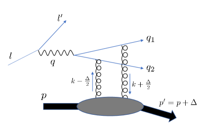
Figure 1: Exclusive dijet production in electron-proton scattering.

In this section, we calculate the cross section of longitudinal double spin asymmetry in exclusive dijet production. A brief summary of the result has been reported in our previous publication Bhattacharya et al. (2022a). The process is depicted in Fig. 1. At high center-of-mass energies, the dominant contribution comes from the two-gluon exchange diagrams. The quark exchange diagrams will be discussed in a later section.

We assume that both the incoming proton and lepton are longitudinally polarized with helicity $h_{p}=\pm 1$ and $h_{l}=\pm 1$, respectively. We write the cross section $d\sigma^{h_{p}h_{l}}$ in the form

$$d\sigma^{h_{p}h_{l}}=d\sigma_{0}+h_{p}d\sigma_{\rm SSA}+h_{l}d\sigma_{\rm BSA}+h_{p}h_{l}d\sigma_{\rm DSA},$$ (29)

where the last three terms represent single spin asymmetry (SSA), beam spin asymmetry (BSA) and double spin asymmetry (DSA). The previous works Ji et al. (2017); Hatta et al. (2017) looked for signals of OAM in SSA, while our main focus here is DSA which can be isolated by forming the linear combination

$$d\sigma_{\rm DSA}=\frac{1}{4}(d\sigma^{++}-d\sigma^{+-}-d\sigma^{-+}+d\sigma^{--}).$$ (30)

The incoming proton has momentum $p^{\mu}\approx((1+\xi)P^{+},0,0_{\perp})$, where $\xi$ is the skewness variable, and scatters elastically with momentum transfer $\Delta^{\mu}=(-2\xi P^{+},0,\Delta_{\perp})$ with $\Delta_{\perp}=|\Delta_{\perp}|(\cos\phi_{\Delta_{\perp}},\sin\phi_{\Delta_{\perp}})$. The virtual photon’s momentum is taken in the form

$$q^{\mu}=\left(-\frac{Q}{\sqrt{2}},\frac{Q}{\sqrt{2}},0_{\perp}\right),$$ (31)

with $q^{2}=-Q^{2}$. In the present frame, the incoming lepton momentum is given by

$$l^{\mu}=\left(\frac{Q(1-y)}{\sqrt{2}y},\frac{Q}{\sqrt{2}y},\frac{Q\sqrt{1-y}}{y}n_{\perp}\right),$$ (32)

where $y=p\cdot q/p\cdot l$ is the usual variable in DIS and $n_{\perp}=(\cos\phi_{l_{\perp}},\sin\phi_{l_{\perp}})$ is a unit vector in the transverse plane. The lepton mass is neglected so that the lepton spin vector is $s^{\mu}\approx h_{l}l^{\mu}$. The center-of-mass energies of the $ep$ and $\gamma^{*}p$ collisions are denoted by $s_{ep}=(p+l)^{2}$ and $W^{2}=(p+q)^{2}=M^{2}-Q^{2}+ys_{ep}$, respectively.

The signal of OAM proposed in Bhattacharya et al. (2022a) is an azimuthal correlation of the form

$$d\sigma_{\rm DSA}\propto\Delta_{\perp}\cdot l_{\perp}=|\Delta_{\perp}||l_{\perp}|\cos(\phi_{\Delta_{\perp}}-\phi_{l_{\perp}}),$$ (33)

measured in coincidence with the production of two jets (dijet) whose azimuthal angle is integrated over. We assume $\Delta_{\perp}$ is small and keep only linear terms in $\Delta_{\perp}$. Under this assumption, we parameterize the momenta of the final state quark and antiquark as

$$\begin{split}&q_{1}^{\mu}=\frac{q_{\perp}^{2}+\mu^{2}}{4\xi\bar{z}}n^{\mu}+\frac{2\xi\bar{z}q_{\perp}^{2}}{q_{\perp}^{2}+\mu^{2}}\left(1-2z\frac{q_{\perp}\cdot\Delta_{\perp}}{q_{\perp}^{2}}\right)P^{\mu}+\delta^{\mu}_{i}(q_{\perp}^{i}-z\Delta^{i}_{\perp}),\\ &q_{2}^{\mu}=\frac{q_{\perp}^{2}+\mu^{2}}{4\xi z}n^{\mu}+\frac{2\xi zq_{\perp}^{2}}{q_{\perp}^{2}+\mu^{2}}\left(1+2\bar{z}\frac{q_{\perp}\cdot\Delta_{\perp}}{q_{\perp}^{2}}\right)P^{\mu}+\delta^{\mu}_{i}(-q_{\perp}^{i}-\bar{z}\Delta^{i}_{\perp}),\end{split}$$ (34)

where $\mu^{2}\equiv z\bar{z}Q^{2}$. $n^{\mu}=\delta^{\mu}_{-}/P^{+}$ and $P^{\mu}=\delta^{\mu}_{+}P^{+}$ with $n\cdot P=1$ are orthogonal light-like vectors. The condition $q_{1}^{2}=q_{2}^{2}=0$ is satisfied to linear order in $\Delta_{\perp}$. We have introduced the common variables $z=P\cdot q_{1}/P\cdot q=q_{1}^{-}/q^{-}$ and $\bar{z}\equiv 1-z=q_{2}^{-}/q^{-}$ denoting the longitudinal momentum fractions of the virtual photon carried by the quark and the antiquark, respectively. The skewness variable is related to $q_{\perp}$ as

$$\xi(q^{2}_{\perp}) =\dfrac{q^{2}_{\perp}+\mu^{2}}{-q^{2}_{\perp}+\mu^{2}+2z\overline{z}W^{2}}.$$ (35)

At high center-of-mass energy ($W\sim 100$ GeV at the EIC), typically $\xi\ll 1$.

The spin-dependent part of the lepton tensor is

$$L^{\mu\nu}=\sum_{s^{\prime}}\bar{u}(ls)\gamma^{\mu}u(l^{\prime}s^{\prime})\bar{u}(l^{\prime}s^{\prime})\gamma^{\nu}u(ls)\sim-2i\epsilon^{\rho\tau\mu\nu}s_{\rho}q_{\tau}=-2ih_{l}\epsilon^{\rho\tau\mu\nu}l_{\rho}q_{\tau}.$$ (36)

Since the observable (33) depends on $\phi_{l_{\perp}}$, the index $\rho$ has to be transverse. On the other hand, the index $\tau$ is longitudinal (see (31)). This means that either $\mu$ or $\nu$ must be transverse and the other longitudinal. In other words, we are after the interference effect between amplitudes with longitudinally polarized and transversely polarized virtual photons. At the same time, the cross section also encodes interference between twist-two and twist-three amplitudes because the dependence on $\Delta_{\perp}$ shows up only at the twist-three level. Let us thus denote the longitudinal ($L$) and transverse ($T$) amplitudes as

$$A_{L}\equiv\epsilon_{\mu}^{L}A^{\mu}=A_{L}^{2}+A_{L}^{3},\qquad A_{T\lambda}\equiv\epsilon^{i}_{T\lambda}A^{i}=\epsilon_{T\lambda}^{i}(A_{T}^{2i}+A_{T}^{3i}),$$ (37)

where $\lambda=1,2$ is a label for the two transverse polarization vectors and

$$\epsilon_{\mu}^{L}=\frac{1}{Q}\left(q_{\mu}+\frac{Q^{2}}{p\cdot q}p_{\mu}\right),$$ (38)

is the longitudinal photon polarization vector. The term proportional to $q^{\mu}$ can be omitted due to gauge invariance. The superscripts 2 and 3 denote the twist at which the amplitude is evaluated. The relevant part of the cross section is then given by

$$L^{\mu\nu}A^{*}_{\mu}A_{\nu} \sim -\sum_{\lambda=1,2}L^{\mu\nu}(\epsilon^{L}_{\mu}\epsilon_{\nu}^{T\lambda*}A^{*}_{L}A^{\lambda}_{T}+\epsilon^{T\lambda}_{\mu}\epsilon_{\nu}^{L}A_{T}^{\lambda*}A_{L})$$ (39)

$$= 2ih_{l}|l_{\perp}|\epsilon_{ij}(A_{L}^{2*}A^{3i}_{T}+A_{L}^{3*}A^{2i}_{T}-A^{2i*}_{T}A^{3}_{L}-A^{3i*}_{T}A^{2}_{L})n_{\perp}^{j}$$

$$= 4h_{l}|l_{\perp}|\epsilon_{ij}{\rm Re}(iA_{L}^{2*}A^{3i}_{T}-iA^{2i*}_{T}A^{3}_{L})n_{\perp}^{j}.$$

Dirac traces involving the incoming and outgoing nucleon spinors, as well as the produced $q\bar{q}$ spinors are understood. The cosine angular correlation (33) originates from the following structure

$${\rm Re}(iA_{L}^{2*}A^{3i}_{T}-iA^{2i*}_{T}A^{3}_{L})\sim h_{p}\epsilon^{ik}\Delta^{k}_{\perp}.$$ (40)

As observed in Bhattacharya et al. (2022a), there are two different but equally important (at least parametrically) contributions to (40). A factor of $\Delta_{\perp}$ can arise either from the soft (GTMD) part or the hard scattering part. The former is directly related to the gluon OAM which we are mainly interested in, and the latter is the so-called kinematical twist-three effect which involves only twist-two GPDs (hence unrelated to GTMDs). We shall discuss these contributions in the next subsection.

III.2 Outline of the calculation

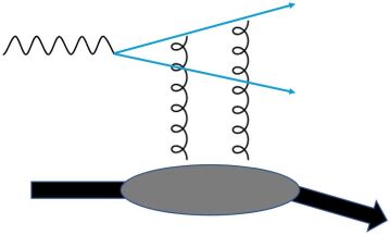
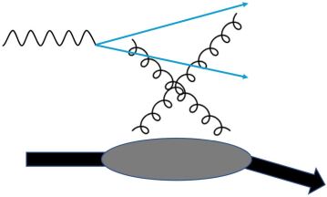
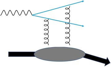
Figure 2: Presented are the leading-order Feynman diagrams depicting exclusive dijet production initiated by gluons. The complementary set of three diagrams, with the quark lines exchanged, is implicit.

In the two-gluon exchange approximation, the hadronic part of the scattering amplitude can be written as

$$iA_{L/T}=\frac{-ig^{2}e_{em}e_{q}C_{F}}{\left(N_{c}^{2}-1\right)P^{+}}\int\frac{dz^{-}d^{2}z_{\perp}}{\left(2\pi\right)^{3}}\int\frac{dx}{x^{2}-\xi^{2}}\int d^{2}k_{\perp}e^{ixP^{+}z^{-}-ik_{\perp}\cdot z_{\perp}}D^{L/T}_{\mu\nu}\left\langle p^{\prime}\left|F^{+\mu}\left(-\frac{z}{2}\right)F^{+\nu}\left(\frac{z}{2}\right)\right|p\right\rangle.$$ (41)

Here and below, $\frac{1}{x^{2}-\xi^{2}}$ is a shorthand notation for

$$\frac{1}{(x-\xi+i\epsilon)(x+\xi-i\epsilon)}.$$ (42)

The hard part $D_{\mu\nu}$ consists of six diagrams as shown in Fig. 2. Explicitly,

$$D^{L/T}_{\mu\nu} = \epsilon^{\rho}_{L/T}\bar{u}(q_{1})\Biggl{[}\gamma_{\nu}\frac{1}{{\ooalign{\hfil/\hfil\crcr$q$}}_{1}+{\ooalign{\hfil/\hfil\crcr$k$}}+{\ooalign{\hfil/\hfil\crcr$\Delta$}}/2}\gamma_{\mu}\frac{1}{{\ooalign{\hfil/\hfil\crcr$q$}}_{1}+{\ooalign{\hfil/\hfil\crcr$\Delta$}}}\gamma_{\rho}+\gamma_{\rho}\frac{1}{{\ooalign{\hfil/\hfil\crcr$q$}}_{2}+{\ooalign{\hfil/\hfil\crcr$\Delta$}}}\gamma_{\mu}\frac{1}{{\ooalign{\hfil/\hfil\crcr$q$}}_{2}+{\ooalign{\hfil/\hfil\crcr$k$}}+{\ooalign{\hfil/\hfil\crcr$\Delta$}}/2}\gamma_{\nu}$$ (109)

$$\qquad\quad+\gamma_{\mu}\frac{1}{{\ooalign{\hfil/\hfil\crcr$q$}}_{1}-{\ooalign{\hfil/\hfil\crcr$k$}}+{\ooalign{\hfil/\hfil\crcr$\Delta$}}/2}\gamma_{\nu}\frac{1}{{\ooalign{\hfil/\hfil\crcr$q$}}_{1}+{\ooalign{\hfil/\hfil\crcr$\Delta$}}}\gamma_{\rho}+\gamma_{\rho}\frac{1}{{\ooalign{\hfil/\hfil\crcr$q$}}_{2}+{\ooalign{\hfil/\hfil\crcr$\Delta$}}}\gamma_{\nu}\frac{1}{{\ooalign{\hfil/\hfil\crcr$q$}}_{2}-{\ooalign{\hfil/\hfil\crcr$k$}}+{\ooalign{\hfil/\hfil\crcr$\Delta$}}/2}\gamma_{\mu}$$

$$\qquad\quad-\gamma_{\mu}\frac{1}{{\ooalign{\hfil/\hfil\crcr$q$}}_{1}-{\ooalign{\hfil/\hfil\crcr$k$}}+{\ooalign{\hfil/\hfil\crcr$\Delta$}}/2}\gamma_{\rho}\frac{1}{{\ooalign{\hfil/\hfil\crcr$q$}}_{2}+{\ooalign{\hfil/\hfil\crcr$k$}}+{\ooalign{\hfil/\hfil\crcr$\Delta$}}/2}\gamma_{\nu}-\gamma_{\nu}\frac{1}{{\ooalign{\hfil/\hfil\crcr$q$}}_{1}+{\ooalign{\hfil/\hfil\crcr$k$}}+{\ooalign{\hfil/\hfil\crcr$\Delta$}}/2}\gamma_{\rho}\frac{1}{{\ooalign{\hfil/\hfil\crcr$q$}}_{2}-{\ooalign{\hfil/\hfil\crcr$k$}}+{\ooalign{\hfil/\hfil\crcr$\Delta$}}/2}\gamma_{\mu}\Biggr{]}v(q_{2}),$$

where $k^{\mu}=(xP^{+},0,k_{\perp})$. One then projects onto the symmetric (unpolarized) and antisymmetric (polarized) parts in the gluon transverse indices

$$D_{\mu\nu}\langle F^{+\mu}F^{+\nu}\rangle = \frac{1}{2}g_{\mu\nu}^{\perp}D^{\mu\nu}\langle g_{\alpha\beta}^{\perp}F^{+\alpha}F^{+\beta}\rangle+\frac{1}{2}\epsilon^{\perp}_{\mu\nu}D^{\mu\nu}\langle\epsilon^{\perp}_{\alpha\beta}F^{+\alpha}F^{+\beta}\rangle$$ (110)

$$\sim \frac{1}{2}\delta_{ij}D_{ij}xf_{g}+\frac{1}{2}\epsilon_{ij}D_{ij}ix\tilde{f}_{g},$$

where $g_{\mu\nu}^{\perp}=g_{\mu\nu}-P_{\mu}n_{\nu}-P_{\nu}n_{\mu}$ and $\epsilon_{\mu\nu}^{\perp}=\epsilon_{\mu\nu\alpha\beta}P^{\alpha}n^{\beta}$.

Our basic strategy is to expand $D_{ij}$ in powers of $k_{\perp}$ and $\Delta_{\perp}$ to linear order

$$D_{ij}(k_{\perp},\Delta_{\perp})\approx D_{ij}(0_{\perp},0_{\perp})+\left.\frac{\partial D_{ij}(k_{\perp},0_{\perp})}{\partial k_{\perp}^{l}}\right|_{k=0}k_{\perp}^{l}+\left.\frac{\partial D_{ij}(0_{\perp},\Delta_{\perp})}{\partial\Delta_{\perp}^{l}}\right|_{\Delta=0}\Delta_{\perp}^{l}.$$ (111)

To do so, we need to expand each building block of (109). For example, the first denominator in (109) becomes

$$\frac{1}{(q_{1}+k+\Delta/2)^{2}} \approx \frac{1}{\frac{q_{\perp}^{2}+\mu^{2}}{2\xi\bar{z}}(x-\xi)-2q_{\perp}\cdot k_{\perp}-q_{\perp}\cdot\Delta_{\perp}}$$ (112)

$$\approx \frac{2\xi\bar{z}}{(q_{\perp}^{2}+\mu^{2})(x-\xi)}+\frac{(2\xi\bar{z})^{2}}{(q_{\perp}^{2}+\mu^{2})^{2}(x-\xi)^{2}}\left(2q_{\perp}\cdot k_{\perp}+q_{\perp}\cdot\Delta_{\perp}\right).$$

When (111) is substituted into (110), the integral $\int d^{2}k_{\perp}k_{\perp}^{l}xf_{g}\sim\epsilon^{lm}\Delta_{\perp}^{m}L_{g}$ establishes a connection to the gluon OAM (13). On the other hand, the first and last terms in (111) are independent of $k_{\perp}$, so these terms lead to the twist-two gluon GPDs $\int d^{2}k_{\perp}xf_{g}\sim H_{g},E_{g}$ and $\int d^{2}k_{\perp}x\tilde{f}_{g}\sim\tilde{H}_{g},\tilde{E}_{g}$. Further squaring the amplitude as in (39), we encounter a number of interference terms. We have considered all the possibilities and found that the angular dependence (33) can come from the following sources

$$H_{g}\otimes\int d^{2}k_{\perp}k^{l}_{\perp}xf_{g},\qquad H_{g}\otimes\tilde{H}_{g},\qquad\tilde{H}_{g}\otimes\int d^{2}k_{\perp}k^{l}_{\perp}x\tilde{f}_{g}.$$ (113)

The first term involves the gluon OAM and the second term represents the kinematical twist-three effect mentioned above. In Bhattacharya et al. (2022a), we neglected the third term assuming that, at high energy $\xi\ll 1$, the product of the polarized GPD and the polarized GTMD would be subleading. In the following, we shall also calculate the third term to check the validity of this assumption.

First, consider the twist-two ($k_{\perp}=\Delta_{\perp}=0$) term in (111). Applying the symmetric projection $\delta_{ij}D_{ij}$ (denoted by a superscript $\delta$), one finds Braun and Ivanov (2005)

$$\begin{split}&iA^{2\delta}_{T}=-\dfrac{ig^{2}e_{em}e_{q}}{N_{c}}\frac{\bar{u}(q_{1})\epsilon_{\perp}\cdot\gamma_{\perp}v(q_{2})}{q_{\perp}^{2}+\mu^{2}}\int dx\frac{1}{x^{2}-\xi^{2}}\left(1+\frac{2\xi^{2}(1-2\beta)}{x^{2}-\xi^{2}}\right)\int d^{2}k_{\perp}xf_{g}(x,\xi,k_{\perp},\Delta_{\perp}),\\ &iA^{2\delta}_{L}=\dfrac{ig^{2}e_{em}e_{q}}{N_{c}}\frac{Q}{(q_{\perp}^{2}+\mu^{2})q^{-}}\bar{u}(q_{1})\gamma^{-}v(q_{2})\int dx\frac{1}{x^{2}-\xi^{2}}\left(1+\frac{4\xi^{2}(1-\beta)}{x^{2}-\xi^{2}}\right)\int d^{2}k_{\perp}xf_{g}(x,\xi,k_{\perp},\Delta_{\perp}),\end{split}$$ (116)

where

$$\beta\equiv\frac{\mu^{2}}{q_{\perp}^{2}+\mu^{2}}.$$ (117)

As we shall discuss later, $\beta$ is related to the invariant mass of the dijet. It is actually a commonly used variable in the context of diffractive DIS. The following relation is useful throughout the calculation

$$P^{+}q^{-}=\frac{q_{\perp}^{2}+\mu^{2}}{4\xi z\bar{z}}=\frac{q_{\perp}^{2}}{4\xi z\bar{z}(1-\beta)}.$$ (118)

The antisymmetric contraction (denoted by a superscript $\epsilon$) gives

$$\begin{split}&iA_{T}^{2\epsilon}=\dfrac{ig^{2}e_{em}e_{q}}{N_{c}}\frac{\bar{u}(q_{1})\epsilon_{\perp}\times\gamma_{\perp}v(q_{2})}{q_{\perp}^{2}+\mu^{2}}\int dx\frac{2\xi x}{(x^{2}-\xi^{2})^{2}}\int d^{2}k_{\perp}x\tilde{f}_{g}(x,\xi,k_{\perp},\Delta_{\perp}),\\ &iA_{L}^{2\epsilon}=0.\end{split}$$ (119)

The $k_{\perp}$-integrals in (116) and (119) convert the gluon GTMDs into the gluon GPDs $H_{g},E_{g},\tilde{H}_{g},\tilde{E}_{g}$. Further integration over $x$ yields the following moments of the GPDs

$$\begin{split}&{\cal H}^{(1)}_{g}(\xi)=\int^{1}_{-1}dx\frac{H_{g}(x,\xi)}{x^{2}-\xi^{2}},\qquad{\cal E}^{(1)}_{g}(\xi)=\int^{1}_{-1}dx\frac{E_{g}(x,\xi)}{x^{2}-\xi^{2}},\\ &{\cal H}^{(2)}_{g}(\xi)=\int^{1}_{-1}dx\frac{\xi^{2}H_{g}(x,\xi)}{(x^{2}-\xi^{2})^{2}},\qquad{\cal E}^{(2)}_{g}(\xi)=\int^{1}_{-1}dx\frac{\xi^{2}E_{g}(x,\xi)}{(x^{2}-\xi^{2})^{2}},\\ &\tilde{{\cal H}}^{(2)}_{g}(\xi)=\int^{1}_{-1}dx\frac{x\tilde{H}_{g}(x,\xi)}{(x^{2}-\xi^{2})^{2}},\qquad\tilde{{\cal E}}^{(2)}_{g}(\xi)=\int^{1}_{-1}dx\frac{x\tilde{E}_{g}(x,\xi)}{(x^{2}-\xi^{2})^{2}}.\end{split}$$ (120)

These integrals are well defined as long as the GPDs and their first derivatives are continuous at $x=\pm\xi$, which is usually considered to be the case. Squaring the amplitudes (116), one obtains the cross section of unpolarized dijet production Braun and Ivanov (2005).

We now turn to the twist-three contributions that give rise to the asymmetry (33). The first entry in (113) related to the OAM originates from the second term in (111). The calculation of the amplitude has been done in Ji et al. (2017) in the context of SSA, and the same results are relevant to DSA:

$$\begin{split}iA^{3\delta}_{T}&=-\dfrac{ig^{2}e_{em}e_{q}}{N_{c}}\dfrac{4\xi(\overline{z}-z)}{(q^{2}_{\perp}+\mu^{2})^{2}}\bar{u}(q_{1})\epsilon_{\perp}\cdot\gamma_{\perp}v(q_{2})\\ &\qquad\qquad\times\int dx\dfrac{x}{(x^{2}-\xi^{2})^{2}}\bigg{(}1+\dfrac{4\xi^{2}(1-2\beta)}{x^{2}-\xi^{2}}\bigg{)}\int d^{2}k_{\perp}q_{\perp}\cdot k_{\perp}\,xf_{g}(x,\xi,k_{\perp},\Delta_{\perp})\\[5.69046pt] &\quad-\dfrac{ig^{2}e_{em}e_{q}}{N_{c}}\dfrac{2\xi}{(q^{2}_{\perp}+\mu^{2})q^{-}}\bar{u}(q_{1})\gamma^{-}v(q_{2})\int dx\dfrac{x}{(x^{2}-\xi^{2})^{2}}\int d^{2}k_{\perp}\epsilon_{\perp}\cdot k_{\perp}\,xf_{g}(x,\xi,k_{\perp},\Delta_{\perp}),\\[8.5359pt] iA^{3\delta}_{L}&=\dfrac{ig^{2}e_{em}e_{q}}{N_{c}}\dfrac{4\xi(\overline{z}-z)Q}{(q^{2}_{\perp}+\mu^{2})^{2}q^{-}}\bar{u}(q_{1})\gamma^{-}v(q_{2})\\ &\qquad\qquad\times\int dx\dfrac{x}{(x^{2}-\xi^{2})^{2}}\bigg{(}1+\dfrac{8\xi^{2}(1-\beta)}{x^{2}-\xi^{2}}\bigg{)}\int d^{2}k_{\perp}\,q_{\perp}\cdot k_{\perp}\,xf_{g}(x,\xi,k_{\perp},\Delta_{\perp}).\end{split}$$ (121)

For this contribution, the factor $\Delta_{\perp}$ necessary for the angular dependence (33) emerges from the Dirac trace over the nucleon spinors. Indeed, taking the interference effect between (116) and (121) and summing over the outgoing nucleon spins while fixing the spin of the incoming nucleon, we find

$$\frac{1}{4P^{+}M}{\rm tr}\left[\left(H_{g}\gamma^{+}-\frac{i\sigma^{+\nu}\widetilde{\Delta}_{\nu}}{2M}E_{g}\right)\left({\ooalign{\hfil/\hfil\crcr$p$}}^{\prime}+M\right)\left(F^{g}_{1,1}+i\frac{\sigma^{j+}}{P^{+}}(\widetilde{k}_{\perp}^{j}F^{g}_{1,2}+\widetilde{\Delta}_{\perp}^{j}F^{g}_{1,3})+i\frac{\sigma^{ij}\widetilde{k}_{\perp}^{i}\widetilde{\Delta}_{\perp}^{j}}{M^{2}}F^{g}_{1,4}\right)\left({\ooalign{\hfil/\hfil\crcr$p$}}+M\right)\frac{{\ooalign{\hfil/\hfil\crcr$s$}}\gamma_{5}}{2M}\right]$$ (128)

$$=ih_{p}\frac{1+\xi}{2M^{2}}\epsilon^{ij}k_{\perp}^{i}\Delta_{\perp}^{j}\left[2\left(H_{g}-\frac{\xi^{2}}{1-\xi^{2}}E_{g}\right)F_{1,4}^{g}-E_{g}F_{1,2}^{g}\right].$$ (129)

As indicated by the notations $\widetilde{k}_{\perp},\widetilde{\Delta}_{\perp}$, this can be conveniently evaluated in the symmetric frame where the factor of $1+\xi$ comes from $\tilde{\Delta}_{\perp}=(1+\xi)\Delta_{\perp}$. The product of $k_{\perp}^{i}F_{1,4}^{g}$ from (129) and $k_{\perp}$ from (121) leads to the moment (13) after the $k_{\perp}$ integration. From the $k_{\perp}^{i}F_{1,2}^{g}$ term in (129), we get another moment

$$xO(x,\xi)\equiv\int d^{2}k_{\perp}\frac{k_{\perp}^{2}}{M^{2}}F^{g}_{1,2}(x,\xi).$$ (130)

The notation $O$ is a reminder that the imaginary part of $F_{1,2}^{g}$ is related to the so-called spin-dependent Odderon Zhou (2014); Szymanowski and Zhou (2016). Its second moment at $\xi=0$ is proportional to the $C$-odd three-gluon correlator $\langle P|d_{abc}F_{a}^{+i}F_{b}^{+j}F_{c}^{+i}|P\rangle$ Ji (1992) relevant to transverse single spin asymmetry Zhou (2014). The real part of $F_{1,2}^{g}$ is proportional to $\xi$ (at $\Delta_{\perp}=0$, see (21)) so it is suppressed when $\xi\ll 1$.

The subsequent integration over $x$ in (121) yields the following moments

$${\cal L}^{(2)}_{g}(\xi) = \int^{1}_{-1}dx\frac{x^{2}L_{g}(x,\xi)}{(x^{2}-\xi^{2})^{2}},\qquad{\cal O}^{(2)}(\xi)=\int^{1}_{-1}dx\frac{x^{2}O(x,\xi)}{(x^{2}-\xi^{2})^{2}},$$ (131)

$${\cal L}^{(3)}_{g}(\xi) = \int^{1}_{-1}dx\frac{\xi^{2}x^{2}L_{g}(x,\xi)}{(x^{2}-\xi^{2})^{3}},\qquad{\cal O}^{(3)}(\xi)=\int^{1}_{-1}dx\frac{\xi^{2}x^{2}O(x,\xi)}{(x^{2}-\xi^{2})^{3}}.$$ (132)

We immediately notice triple poles at $x=\pm\xi$ which were absent in the twist-two amplitudes (120). In order for the $x$-integrals in (132) to be well-defined, the second derivative of $L_{g}(x,\xi)$ and $O(x,\xi)$ must be continuous at $x=\pm\xi$. It is known that such a condition can be violated for gluonic GPDs, and this in fact signals the violation of collinear factorization. We postpone this issue until the next subsection where the problem becomes sharper. In the meantime, let us just point out that all the terms in (121) which contain triple poles can be eliminated by setting $z=\bar{z}=\frac{1}{2}$, that is, when the produced jets are symmetric.

Next, the second entry in (113) comes from the last term in (111) obtained by setting $k_{\perp}=0$ and keeping one factor of $\Delta_{\perp}$ in the hard part. Accordingly, in the soft part one can set $\Delta_{\perp}=0$ and integrate over $k_{\perp}$, after which GTMDs reduce to GPDs in both the amplitude and the complex-conjugate amplitude. The structure (40) then arises from interference between the unpolarized and polarized amplitudes. The asymmetry is therefore proportional to

$$\frac{1}{4(P^{+})^{2}}{\rm tr}\left[\left(H_{g}\gamma^{+}-\frac{i\sigma^{+\nu}\Delta_{\nu}}{2M}E_{g}\right)\left({\ooalign{\hfil/\hfil\crcr$p$}}^{\prime}+M\right)\left(i\gamma_{5}\gamma^{+}\widetilde{H}_{g}-i\frac{\gamma_{5}\Delta^{+}}{2M}\widetilde{E}_{g}\right)\left({\ooalign{\hfil/\hfil\crcr$p$}}+M\right)\frac{{\ooalign{\hfil/\hfil\crcr$s$}}\gamma_{5}}{2M}\right]$$ (139)

$$=ih_{p}\left(1-\xi^{2}\right)\left(H_{g}-\frac{\xi^{2}}{1-\xi^{2}}E_{g}\right)\left(\widetilde{H}_{g}-\frac{\xi^{2}}{1-\xi^{2}}\widetilde{E}_{g}\right).$$ (140)

The calculation of the hard part is straightforward but quite cumbersome, since one has to consider many cases: longitudinal/transverse photons; twist-two/twist-three amplitudes; symmetric/antisymmetric projections (110). Moreover, in addition to the explicit $\Delta_{\perp}$-dependence coming from the expansion of the propagators, cf., (112), the factor of $\Delta_{\perp}$ can also come from the Dirac trace over the final state quark spinors $\bar{u}(q_{1}),v(q_{2})$ since $q_{1,2}$ depend on $\Delta_{\perp}$, see (34). Therefore, in practice it is more advantageous to expand the squared amplitude in $\Delta_{\perp}$ instead of the amplitude itself. Schematically, (39) should be generalized as

$${\rm Re}\left[iA_{L}^{2\delta*}A_{T}^{3\epsilon i}+iA_{L}^{3\delta*}A_{T}^{2\epsilon i}-iA_{T}^{2\delta i*}A_{L}^{3\epsilon}-iA_{T}^{3\delta i*}A_{L}^{2\epsilon}+i(A_{L}^{\delta*}A_{T}^{\epsilon i})^{3}-i(A_{T}^{\delta i*}A_{L}^{\epsilon})^{3}\right].$$ (141)

In the last two terms, the factor of $\Delta_{\perp}$ comes from the squared hard amplitude including the final state $q\bar{q}$ spinors. In Bhattacharya et al. (2022a) we have performed this calculation analytically for the special case $z=\frac{1}{2}$. For generic values of $z$, we have developed a Mathematica program to facilitate the calculation.

Finally, we turn to the third entry in (113). This can be calculated in the same way as the OAM contribution except that $\delta_{ij}\to\epsilon_{ij}$ everywhere. The twist-three hard amplitudes read

$$\begin{split}iA^{3\epsilon}_{T}&=-\dfrac{ig^{2}e_{em}e_{q}}{N_{c}}\int\frac{dx}{(x^{2}-\xi^{2})^{2}}\Biggl{[}\left\{\bar{u}(q_{1})\epsilon_{\perp}\times\gamma_{\perp}v(q_{2})(z-\bar{z})\left(3+\frac{4\xi^{2}}{x^{2}-\xi^{2}}\right)+\bar{u}(q_{1})\gamma^{-}v(q_{2})\frac{2q_{\perp}\times\epsilon_{\perp}}{q^{-}}\right\}\\ &\qquad\qquad\qquad\qquad\qquad\times\frac{4\xi^{2}}{(q_{\perp}^{2}+\mu^{2})^{2}}\int d^{2}k_{\perp}q_{\perp}\cdot k_{\perp}\,ix\tilde{f}_{g}(x,\xi,k_{\perp},\Delta_{\perp})\\[5.69046pt] &\qquad\qquad\qquad\quad+\bar{u}(q_{1})\gamma^{-}v(q_{2})\frac{2\xi^{2}}{(q_{\perp}^{2}+\mu^{2})q^{-}}\int d^{2}k_{\perp}\epsilon_{\perp}\times k_{\perp}\,ix\tilde{f}_{g}(x,\xi,k_{\perp},\Delta_{\perp})\Biggr{]},\\[8.5359pt] iA^{3\epsilon}_{L}&=-\dfrac{ig^{2}e_{em}e_{q}}{N_{c}}\frac{4\xi^{2}Q}{q^{-}(q_{\perp}^{2}+\mu^{2})^{2}}\bar{u}(q_{1})\gamma_{5}\gamma^{-}v(q_{2})\int\dfrac{dx}{(x^{2}-\xi^{2})^{2}}\int d^{2}k_{\perp}\,q_{\perp}\cdot k_{\perp}\,x\tilde{f}_{g}(x,\xi,k_{\perp},\Delta_{\perp}).\end{split}$$ (142)

In the soft part, the nucleon spinor sum gives

$$\frac{-i}{4P^{+}M}{\rm tr}\left[\left(\tilde{H}_{g}\gamma_{5}\gamma^{+}+\tilde{E}_{g}\frac{\gamma_{5}\Delta^{+}}{2M}\right)\left({\ooalign{\hfil/\hfil\crcr$p$}}^{\prime}+M\right)\left(\frac{\epsilon_{ij}\widetilde{k}_{\perp}^{i}\widetilde{\Delta}_{\perp}^{j}}{M^{2}}G^{g}_{1,1}-\frac{\sigma^{i+}\gamma_{5}}{P^{+}}(\widetilde{k}_{\perp}^{i}G^{g}_{1,2}+\widetilde{\Delta}_{\perp}^{i}G^{g}_{1,3})-\sigma^{+-}\gamma_{5}G^{g}_{1,4}\right)\left({\ooalign{\hfil/\hfil\crcr$p$}}+M\right)\frac{{\ooalign{\hfil/\hfil\crcr$s$}}\gamma_{5}}{2M}\right]$$ (149)

$$=ih_{p}\frac{1+\xi}{2M^{2}}\left(2\left(\tilde{H}_{g}-\frac{\xi^{2}}{1-\xi^{2}}\tilde{E}_{g}\right)G^{g}_{1,1}-\xi\tilde{E}_{g}G^{g}_{1,2}\right)\epsilon_{ij}k_{\perp}^{i}\Delta^{j}_{\perp}.$$ (150)

The $k_{\perp}$ integrals then lead to the moments

$$xC_{g}(x,\xi)\equiv\int d^{2}k_{\perp}\frac{k_{\perp}^{2}}{M^{2}}G_{1,1}^{g}(x,\xi),\qquad xC^{\prime}_{g}(x,\xi)\equiv-\int d^{2}k_{\perp}\frac{k_{\perp}^{2}}{M^{2}}G_{1,2}^{g}(x,\xi).$$ (151)

With these definitions, $C_{g}(x,\xi)$ and $C^{\prime}_{g}(x,\xi)$ are odd functions in $x$. [Note that $H_{g}(x,\xi),x\tilde{H}_{g}(x,\xi),L_{g}(x,\xi)$ and $O(x,\xi)$ are all even functions in $x$.] Similarly to the quark case Lorce and Pasquini (2011), we interpret $C_{g}(x,\xi=0)$ as the gluons’ spin-orbit correlation. On the other hand, $C^{\prime}_{g}(x,\xi=0)$ is related to another $C$-odd three-gluon correlator $\langle d_{abc}F_{a}^{+i}F_{b}^{+j}\tilde{F}_{c}^{+i}\rangle$. Very little is known about these distributions except that they appear in specific exclusive reactions Bhattacharya et al. (2022b); Boussarie et al. (2018).

Let us provide quick insights into the characteristics of $C_{g}(x)$ which allows for a quantitative estimate sufficient for the present purpose, leaving a more detailed analysis for future work. First, despite being associated with the polarized gluon operator $\tilde{F}^{+\mu}F^{+}_{\ \mu}$, $C_{g}(x)$ has little to do with the parent hadron spin and exists even for spinless hadrons. Second, just like $L_{g}(x)$ (see (16)), using the equations of motion one can express $C_{g}(x)$ as the sum of the Wandzura-Wilczek (WW) part and the genuine twist-three part. Adapting the method in Hatta and Yoshida (2012), we have computed the WW part

$$C_{g}(x) = x\int_{x}^{\epsilon(x)}\frac{dx^{\prime}}{x^{\prime 2}}\tilde{H}_{g}(x^{\prime})-2x\int_{x}^{\epsilon(x)}\frac{dx^{\prime}}{x^{\prime 2}}G(x^{\prime})+\cdots.$$ (152)

(152) allows us to infer the small-$x$ behavior of $C_{g}(x)$. Clearly, the second term dominates at small-$x$ because, roughly, $\tilde{H}_{g}(x)=x\Delta G(x)\sim x^{2}G(x)$. Assuming the power-law (17), we find

$$C_{g}(x)\approx-\frac{2}{2+c}G(x)\approx-G(x),$$ (153)

where the last expression follows if the exponent is perturbatively small $c\propto\alpha_{s}\ll 1$. Since $G(x)$ is positive at small-$x$, $C_{g}(x)$ is negative, meaning that the helicity and OAM of individual gluons are anti-aligned (have opposite signs) Lorce and Pasquini (2011) at small-$x$, in accordance with the theoretical prediction (18). (153) also shows that $C_{g}(x)$ grows strongly in the small-$x$ region. This is consistent with an independent analysis based on an effective theory of small-$x$ QCD Boer et al. (2018); S. Bhattacharya, R. Boussarie, and Y. Hatta (2024).

III.3 The result

Let us introduce the convenient notation

$$F_{g}\equiv H_{g}-\frac{\xi^{2}}{1-\xi^{2}}E_{g},\qquad\tilde{F}_{g}\equiv\tilde{H}_{g}-\frac{\xi^{2}}{1-\xi^{2}}\tilde{E}_{g},$$ (154)

for the linear combinations of GPDs which appear in the Dirac traces (129), (140) (150). Similarly to (120), we define ($n=1,2,3$)

$${\cal F}^{(n)}_{g}(\xi)=\int_{-1}^{1}dx\frac{\xi^{2(n-1)}F_{g}(x,\xi)}{(x^{2}-\xi^{2})^{n}},\qquad\tilde{\cal F}^{(n)}_{g}(\xi)=\int_{-1}^{1}dx\frac{\xi^{2(n-2)}x\tilde{F}_{g}(x,\xi)}{(x^{2}-\xi^{2})^{n}},$$ (155)

and

$${\cal C}_{g}^{(2)}(\xi)=\int_{-1}^{1}dx\frac{\xi^{2}xC_{g}(x,\xi)}{(x^{2}-\xi^{2})^{2}},\qquad{\cal C}^{\prime(2)}_{g}(\xi)=\int_{-1}^{1}dx\frac{\xi^{2}xC^{\prime}_{g}(x,\xi)}{(x^{2}-\xi^{2})^{2}}.$$ (156)

Using these moments, our final result for the cross section can be expressed as

$$\dfrac{d\sigma_{\rm DSA}}{dydQ^{2}d\phi_{l_{\perp}}dzdq_{\perp}^{2}d^{2}\Delta_{\perp}}=\dfrac{e_{q}^{2}\alpha_{em}^{2}\alpha_{s}^{2}y}{2\pi^{3}Q^{2}N_{c}}\dfrac{\xi(1+\xi)|l_{\perp}||\Delta_{\perp}|\cos(\phi_{l_{\perp}}-\phi_{\Delta_{\perp}})}{z\overline{z}(W^{2}+Q^{2})(W^{2}-M_{J}^{2})(q_{\perp}^{2}+\mu^{2})^{2}}{\rm Re}(\Sigma_{L}+\Sigma_{O}+\Sigma_{h}+\Sigma_{C}),$$ (157)

where the contribution from the gluon OAM is

$$\Sigma_{L} = -\left({\cal F}^{(1)*}_{g}+4(1-\beta){\cal F}^{(2)*}_{g}\right){\cal L}_{g}^{(2)}+(z-\bar{z})^{2}{\cal F}_{g}^{(1)*}\left({\cal L}_{g}^{(2)}+8(1-\beta){\cal L}_{g}^{(3)}\right).$$ (158)

There are also contributions from the ‘odderon’

$$\Sigma_{O} = -\frac{1}{2}\left({\cal E}^{(1)*}_{g}+4(1-\beta){\cal E}^{(2)*}_{g}\right){\cal O}_{g}^{(2)}+\frac{(z-\bar{z})^{2}}{2}{\cal E}_{g}^{(1)*}\left({\cal O}_{g}^{(2)}+8(1-\beta){\cal O}_{g}^{(3)}\right),$$ (159)

and from the gluon helicity

$$\Sigma_{h} = (1-\xi){\cal F}_{g}^{(1)*}\tilde{\cal F}_{g}^{(2)}-(1-\xi)(z-\bar{z})^{2}\Biggl{[}8(1-\beta)\left({\cal F}_{g}^{(1)*}+4(1-\beta){\cal F}_{g}^{(2)*}\right)\tilde{\cal F}^{(3)}_{g}$$ (160)

$$\qquad\qquad+\left((4\beta-3){\cal F}_{g}^{(1)*}+16(1-\beta){\cal F}^{(2)*}_{g}+32(1-\beta)^{2}{\cal F}_{g}^{(3)*}\right)\tilde{\cal F}^{(2)}_{g}\Biggr{]},$$

and from the spin-orbit correlation

$$\Sigma_{C}=2(1-\beta)\left(2{\cal C}_{g}^{(2)*}\tilde{\cal F}_{g}^{(2)}+\xi{\cal C}^{\prime(2)*}_{g}\tilde{\cal E}_{g}^{(2)}\right).$$ (161)

Importantly $\Sigma_{h}$ contains integrals with triple poles

$$\begin{split}&{\cal H}_{g}^{(3)}(\xi)=\int_{-1}^{1}dx\frac{\xi^{4}H_{g}(x,\xi)}{(x^{2}-\xi^{2})^{3}},\qquad{\cal E}_{g}^{(3)}(\xi)=\int_{-1}^{1}dx\frac{\xi^{4}E_{g}(x,\xi)}{(x^{2}-\xi^{2})^{3}},\\ &\tilde{\cal H}_{g}^{(3)}(\xi)=\int_{-1}^{1}dx\frac{\xi^{2}x\tilde{H}_{g}(x,\xi)}{(x^{2}-\xi^{2})^{3}},\qquad\tilde{\cal E}_{g}^{(3)}(\xi)=\int_{-1}^{1}dx\frac{\xi^{2}x\tilde{E}_{g}(x,\xi)}{(x^{2}-\xi^{2})^{3}},\end{split}$$ (162)

These are similar to the integrals which we encountered before (132) and are contained in $\Sigma_{L},\Sigma_{O}$. They are well-defined if the second derivative of $H_{g}$, etc, are continuous at $x=\pm\xi$. Unfortunately, however, this condition is known to be violated for $H_{g}$ and $E_{g}$ at least for asymptotically large values of the renormalization scale $\mu_{r}$

$$H_{g}(x,\xi,\mu_{r}),E_{g}(x,\xi,\mu_{r})\sim\theta(\xi-|x|)(x^{2}-\xi^{2})^{2}\qquad(\mu_{r}\to\infty)\,.$$ (163)

Essentially the same problem was previously encountered in the exclusive production of $P$-wave charmonium states Cui et al. (2019) where it was concluded that collinear factorization is violated due to this ‘end-point’ singularity.

In the present problem, clearly the origin of this divergence is the expansion (112) in $k_{\perp}$ and $\Delta_{\perp}$. Had we not done this, the cross section would have been perfectly finite and given in terms of GTMDs (not GPDs). But then we would not be able to exploit the formula (13) to establish a (direct) connection to gluon OAM. Without the detailed knowledge of the behavior of gluon GPDs at $x=\pm\xi$, it is not clear to us whether the integrals (162) are always divergent for realistic values of $\mu_{r}$. However, as already noticed in Bhattacharya et al. (2022a), the integrals with triple poles (162) and (132) always accompany the prefactor $(z-\bar{z})^{2}$, hence they all vanish at $z=\frac{1}{2}$. Since by symmetry $z=\frac{1}{2}$ is a stationary point of the dijet cross section, we can expect that the ${\cal O}(z-\bar{z})^{2}$ ‘curvature’ corrections around $z=\frac{1}{2}$ is moderate in practice and may be neglected to first approximation once the divergence at $z\neq\frac{1}{2}$ is regularized by the the $k_{\perp}$-dependent (GTMD) approach. Further neglecting the odderon contribution and the terms which are explicitly suppressed by powers of $\xi\ll 1$, we arrive at a practically useful formula valid near $z\sim\frac{1}{2}$

$$\Sigma_{L}+\Sigma_{O}+\Sigma_{h}+\Sigma_{C}\approx-\left({\cal H}^{(1)*}_{g}+4(1-\beta){\cal H}^{(2)*}_{g}\right){\cal L}_{g}^{(2)}+\left({\cal H}_{g}^{(1)*}+4(1-\beta){\cal C}_{g}^{(2)*}\right)\tilde{\cal H}_{g}^{(2)}.$$ (164)

In Bhattacharya et al. (2022a), we did not calculate the last term related to the spin-orbit correlation assuming that the contribution from the polarized GTMDs and GPDs are suppressed compared to the unpolarized ones when $\xi\ll 1$. However, the present complete calculation, together with the new formula (152), indicates that this is not the case. From (18) and (152), we expect that ${\cal H}_{g}^{(1)}\sim{\cal H}_{g}^{(2)}\sim{\cal C}_{g}^{(2)}$ and $\tilde{\cal H}_{g}^{(2)}\sim{\cal L}_{g}^{(2)}$ (see Appendix A). We then immediately see that all the terms in (164) are parametrically of the same order.

Let us briefly discuss the impact of the spin-orbit correlation, deferring a numerical estimate to a later section. Previously in Bhattacharya et al. (2022a), we have observed an interesting interplay between the gluon helicity and the gluon OAM in (164). As we show in Appendix A, ${\cal H}_{g}^{(1,2)}$ are dominated by the imaginary part at small-$\xi$ and there is an approximate relation ${\rm Im}{\cal H}_{g}^{(1)}(\xi)\approx-2{\rm Im}{\cal H}^{(2)}_{g}(\xi)$ (cf. Fig. 10). Plugging this into (164) (without the ${\cal C}_{g}^{(2)}$ term), we find that the cross section is roughly proportional to

$$d\sigma_{\rm DSA}\sim{\cal H}^{(1)}_{g}\left(\tilde{\cal H}^{(2)}_{g}+\frac{q_{\perp}^{2}-z\bar{z}Q^{2}}{q_{\perp}^{2}+z\bar{z}Q^{2}}{\cal L}_{g}^{(2)}\right).$$ (165)

Since the helicity and OAM have opposite signs at small-$x$ (18), when $q^{2}_{\perp}\gg z\bar{z}Q^{2}\approx\frac{Q^{2}}{4}$, the two terms in (165) tend to cancel each other, and when $q^{2}_{\perp}\ll z\bar{z}Q^{2}$, they add up. Such an expectation was borne out by the numerical analysis performed in Bhattacharya et al. (2022a). However, this scenario is modified by the spin-orbit term. Due to (153), we expect that ${\cal C}_{g}^{(2)}\approx-{\cal H}_{g}^{(2)}$, and this effectively enhances the coefficient of $\tilde{\cal H}_{g}^{(2)}$ in (164) by a factor $1+2(1-\beta)$. As a result, the impact of the cancellation when $q_{\perp}^{2}\gg Q^{2}/4$ is diminished unless $\beta$ is close to unity.

IV Quark exchange channel

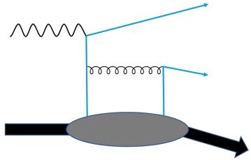
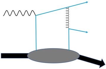
Figure 3: Displayed are the leading-order Feynman diagrams illustrating exclusive dijet production initiated by quarks. The corresponding set of two diagrams, with the quark lines exchanged, is implied.

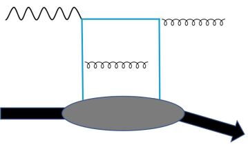
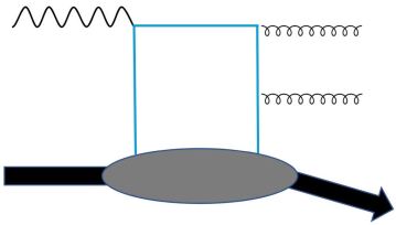
Figure 4: Presented here are the leading-order Feynman diagrams showing exclusive gluon-jet production initiated by quarks. The corresponding pair of diagrams, wherein the quark lines are exchanged, is implied.

We now discuss the quark exchange diagrams for exclusive dijet production. Our original goal was to obtain a formula similar to (157) but this time featuring the quark OAM (9). However, we have encountered an unexpected problem whose resolution is beyond the scope of this work. Therefore, instead of presenting the complete calculation, we will focus on explaining the origin and nature of the problem which may be an interesting observation by itself.

The relevant diagrams are shown in Fig. 3. Their sum is proportional to

$$A^{q}_{L/T} \propto \frac{\epsilon_{L/T}^{\rho}}{(k+\Delta/2+q_{2})^{2}}\bar{u}(q_{1})\Biggl{[}\gamma^{\alpha}\frac{{\ooalign{\hfil/\hfil\crcr$k$}}-\frac{{\ooalign{\hfil/\hfil\crcr$\Delta$}}}{2}+{\ooalign{\hfil/\hfil\crcr$q$}}}{(k-\Delta/2+q)^{2}}\gamma_{\rho}\langle p^{\prime}|\psi\bar{\psi}|p\rangle\gamma_{\alpha}+\gamma_{\rho}\frac{{\ooalign{\hfil/\hfil\crcr$q$}}_{1}-{\ooalign{\hfil/\hfil\crcr$q$}}}{(q_{1}-q)^{2}}\gamma^{\alpha}\langle p^{\prime}|\psi\bar{\psi}|p\rangle\gamma_{\alpha}\Biggr{]}v(q_{2})$$ (187)

$$+\frac{\epsilon_{L/T}^{\rho}}{(k-\Delta/2-q_{1})^{2}}\bar{u}(q_{1})\Biggl{[}\gamma^{\alpha}\langle p^{\prime}|\psi\bar{\psi}|p\rangle\gamma_{\rho}\frac{{\ooalign{\hfil/\hfil\crcr$k$}}+\frac{{\ooalign{\hfil/\hfil\crcr$\Delta$}}}{2}-{\ooalign{\hfil/\hfil\crcr$q$}}}{(k+\Delta/2-q)^{2}}\gamma_{\alpha}+\gamma^{\alpha}\langle p^{\prime}|\psi\bar{\psi}|p\rangle\gamma_{\alpha}\frac{-{\ooalign{\hfil/\hfil\crcr$q$}}_{2}+{\ooalign{\hfil/\hfil\crcr$q$}}}{(-q_{2}+q)^{2}}\gamma_{\rho}\Biggr{]}v(q_{2}).$$

We use the Fierz identity

$$\langle\psi\bar{\psi}\rangle=-\frac{1}{4}\langle\bar{\psi}\gamma^{+}\psi\rangle\gamma^{-}+\frac{1}{4}\langle\bar{\psi}\gamma_{5}\gamma^{+}\psi\rangle\gamma_{5}\gamma^{-}+\cdots,$$ (188)

to project onto the leading twist unpolarized (3) and polarized (4) quark GTMDs. We then extract the twist-two and twist-three parts by expanding to linear order in $k_{\perp}$ and $\Delta_{\perp}$. The twist-two part can be found in Braun and Ivanov (2005). As for the twist-three part, consider for definiteness the longitudinally polarized case ${\ooalign{\hfil/\hfil\crcr$\epsilon$}}_{L}\to\epsilon_{L}^{+}\gamma^{-}$. The unpolarized and polarized amplitudes are given by

$$A^{q,{\rm unpol}}_{L} \propto \frac{\langle\bar{\psi}\gamma^{+}\psi\rangle}{8z\bar{z}\xi(P^{+})^{2}q^{-}}(\bar{u}{\ooalign{\hfil/\hfil\crcr$\epsilon$}}_{L}v)\Biggl{[}\frac{z}{x-\xi}+\frac{\bar{z}}{x+\xi}+\frac{(-z^{2}+\bar{z}^{2})(x^{2}+\xi^{2})-2x\xi(z^{2}+\bar{z}^{2})}{z\bar{z}(x^{2}-\xi^{2})^{2}}\frac{k_{\perp}\cdot q_{\perp}}{P^{+}q^{-}}$$ (192)

$$\qquad\qquad+\frac{(z^{2}-\bar{z}^{2})(x^{3}-3\xi^{2}x)-2\xi^{3}(z^{2}+\bar{z}^{2})}{2\xi z\bar{z}(x^{2}-\xi^{2})^{2}}\frac{q_{\perp}\cdot\Delta_{\perp}}{P^{+}q^{-}}\Biggr{]},$$

$$A_{L}^{q,{\rm pol}} \propto -\frac{\langle\bar{\psi}\gamma_{5}\gamma^{+}\psi\rangle}{8z\bar{z}\xi(P^{+})^{2}q^{-}}(\bar{u}{\ooalign{\hfil/\hfil\crcr$\epsilon$}}_{L}\gamma_{5}v)\Biggl{[}\frac{z}{x-\xi}+\frac{\bar{z}}{x+\xi}+\frac{(-z^{2}+\bar{z}^{2})(x^{2}+\xi^{2})-2x\xi(z^{2}+\bar{z}^{2})}{z\bar{z}(x^{2}-\xi^{2})^{2}}\frac{k_{\perp}\cdot q_{\perp}}{P^{+}q^{-}}$$ (196)

$$\qquad\qquad+\frac{(z^{2}-\bar{z}^{2})(x^{3}-3\xi^{2}x)-2\xi^{3}(z^{2}+\bar{z}^{2})}{2\xi z\bar{z}(x^{2}-\xi^{2})^{2}}\frac{q_{\perp}\cdot\Delta_{\perp}}{P^{+}q^{-}}\Biggr{]}.$$

Integrating the ${\cal O}(k_{\perp})$ term of (192) and (196) over $k_{\perp}$, we obtain the GPD $L_{g}(x,\xi)$ associated with the quark OAM (12) and the quarks’ spin-orbit correlation Lorce and Pasquini (2011), cf., (151)

$$C_{q}(x,\xi)\equiv\int d^{2}k_{\perp}\frac{k_{\perp}^{2}}{M^{2}}G_{1,1}^{q}(x,\xi).$$ (197)

On the other hand, from the ${\cal O}(\Delta_{\perp})$ term of (192) and (196), we obtain the unpolarized and polarized quark GPDs $H_{q}$, $\tilde{H}_{q}$. Up to this point, the discussion is completely parallel with the gluon exchange channel in the previous section. The difference starts to appear after the subsequent integration over $x$ which gives two types of moments with double poles at $x=\pm\xi$

$$(z^{2}-\bar{z}^{2})\int_{-1}^{1}dx\frac{L_{q}(x,\xi)}{(x^{2}-\xi^{2})^{2}}=\frac{z^{2}-\bar{z}^{2}}{2}\int_{-1}^{1}dx\frac{L^{(+)}_{q}(x,\xi)}{(x^{2}-\xi^{2})^{2}},$$ (198)

$$(z^{2}+\bar{z}^{2})\int_{-1}^{1}dx\frac{xL_{q}(x,\xi)}{(x^{2}-\xi^{2})^{2}}=\frac{z^{2}+\bar{z}^{2}}{2}\int_{-1}^{1}dx\frac{xL^{(-)}_{q}(x,\xi)}{(x^{2}-\xi^{2})^{2}},$$ (199)

$$(z^{2}-\bar{z}^{2})\int_{-1}^{1}dx\frac{xH_{q}(x,\xi)}{(x^{2}-\xi^{2})^{2}}=\frac{z^{2}-\bar{z}^{2}}{2}\int_{-1}^{1}dx\frac{xH^{(+)}_{q}(x,\xi)}{(x^{2}-\xi^{2})^{2}},$$ (200)

$$(z^{2}+\bar{z}^{2})\int_{-1}^{1}dx\frac{H_{q}(x,\xi)}{(x^{2}-\xi^{2})^{2}}=\frac{z^{2}+\bar{z}^{2}}{2}\int_{-1}^{1}dx\frac{H^{(-)}_{q}(x,\xi)}{(x^{2}-\xi^{2})^{2}},$$ (201)

where we defined the $C$-parity even $(+)$ and odd $(-)$ quark GPD combinations as

$$L_{q}^{(\pm)}(x,\xi)=L_{q}(x,\xi)\pm L_{q}(-x,\xi),$$

$$H^{(\pm)}_{q}(x,\xi)=H_{q}(x,\xi)\mp H_{q}(-x,\xi).$$ (202)

The $C$-odd contributions arise because the nucleon is not an eigenstate of $C$-parity and the outgoing $q\bar{q}$ pair can be in both $C$-even and $C$-odd states. $L_{q}^{(+)}$ is directly related to the nucleon spin sum rule, while $L_{q}^{(-)}$ can be understood as the OAM of valence quarks.

The problem is that, in the quark channel, it is the double pole that is dangerous for factorization. Indeed, the above integrals are finite provided the first derivative of $H_{q}^{(\pm)},L^{(\pm)}_{q}$ is continuous at $x=\pm\xi$. This condition is known to be violated for $H_{q}^{(\pm)}$ (see Diehl (2003) and references therein), and presumably also for $L_{q}^{(\pm)}$. Note that (200) is exactly the same integral that violates the collinear factorization of the exclusive production of a transversely polarized vector meson Mankiewicz and Piller (2000); Anikin and Teryaev (2003). This integral, together with (198), can be eliminated by setting $z=\frac{1}{2}$ as in the gluon case. Surprisingly, however, the $C$-odd integrals (199), (201) survive even after this approximation and contribute to the cosine modulation (33) after interfering with the twist-two transverse amplitude $A_{T}^{q}$ Braun and Ivanov (2005). We have seen in the previous section that in the gluon case the $C$-odd odderon exchange does not break factorization at least around $z\approx\frac{1}{2}$. Thus the problem is unique to the quark exchange (in contrast to Nabeebaccus et al. (2023)) and exemplifies a novel pattern of factorization breaking.

Another class of diagrams with quark exchange in the $t$ channel could also contribute: diagrams where both jets are initiated by hard gluons (Fig. 4). In that case, by color conservation the gluon pair is on a singlet state and it is thus $C$-even. As a result, the $C$-odd part of the quark distribution is probed and we face the same non-cancellation of double poles even for $z\approx\frac{1}{2}$.

It is expected that, at high energy where $\xi\ll 1$, the quark contribution is subleading compared to the gluon one calculated in the previous section. We therefore neglect it in the numerical analysis below. However, the problem just described appears to pose a challenge if one would like to probe the quark OAM in the large-$x$ region.

V Semi-inclusive diffractive cross section

In a previous publication Bhattacharya et al. (2022a), we have presented a numerical evaluation of the formula (164) (without the last term). While the result cleanly demonstrated the salient features of the cross section such as the interplay between the gluon OAM and helicity contributions, a serious practical challenge was the overall smallness of the cross section. Considering the luminosity of the Electron-Ion Collider, one has to probe the region of jet transverse momentum around $q_{\perp}=1\sim 2$ GeV. The problem is that it is quite difficult to reconstruct jets at such low transverse momentum. One possibility to circumvent this difficulty is to consider dihadron or heavy-quark pair production instead of light-quark dijet production (see, e.g., Reinke Pelicer et al. (2019); Bergabo and Jalilian-Marian (2022); Linek et al. (2023); Fucilla et al. (2023)). In this section, we adopt a different strategy inspired by a recent work Hatta et al. (2022).

One of the advantages of our proposal (as opposed to the earlier proposals Ji et al. (2017); Hatta et al. (2017)) is that the angular modulation $\cos(\phi_{l_{\perp}}-\phi_{\Delta_{\perp}})$ we look for does not depend on the jet azimuthal angle $\phi_{q_{\perp}}$. In fact, $\phi_{q_{\perp}}$ has been integrated over to arrive at the formula (157). It is then tempting to integrate also over $q_{\perp}$. Let us explore this possibility. Experimentally, the parameter $\beta$ introduced in (117), or the invariant mass of the diffractively produced system

$$M_{X}^{2}=\frac{q_{\perp}^{2}}{z\bar{z}}=\frac{1-\beta}{\beta}Q^{2},$$ (203)

is easy to measure since it is not strongly affected by the hadronization effects and does not require jet reconstruction. Moreover, at fixed energy and $Q^{2}$, $\beta$ is in one-to-one correspondence with the skewness parameter

$$\xi=\frac{Q^{2}}{(2\beta-1)Q^{2}+2\beta W^{2}},$$ (204)

upon which the Compton amplitudes, ${\cal H}_{g}^{(1)}(\xi)$ etc., depend. The simplest observable would then be the inclusive cross section $d\sigma/d\beta$ in which $\beta$ is fixed by inserting the constraint

$$1=\int_{0}^{1}d\beta\delta\left(\beta-\frac{z(1-z)Q^{2}}{q_{\perp}^{2}+z(1-z)Q^{2}}\right),$$ (205)

and $q_{\perp}$ and $z$ are integrated over

$$\frac{d\sigma}{dydQ^{2}d\phi_{l_{\perp}}d^{2}\Delta_{\perp}d\beta} = \int_{0}^{1}dz\int_{0}^{\infty}dq_{\perp}^{2}\delta\left(\beta-\frac{z(1-z)Q^{2}}{q_{\perp}^{2}+z(1-z)Q^{2}}\right)f(z,q_{\perp})$$ (206)

$$= \left.\int_{0}^{1}dz\frac{z(1-z)Q^{2}}{\beta}f(z,q_{\perp})\right|_{q_{\perp}^{2}=z(1-z)\frac{1-\beta}{\beta}Q^{2}},$$

where $f$ is the right-hand-side of (157). This is similar to the inclusive diffractive DIS cross section. However, the integral probes the so-called ‘aligned jet’ region $z,\bar{z}\to 0$ where our approximation $z\approx\frac{1}{2}$ breaks down. Besides, at fixed $\beta$, $z,\bar{z}\to 0$ means $q^{2}_{\perp}\to 0$ and $\mu^{2}=z\bar{z}Q^{2}\to 0$, so the twist expansion such as (112) becomes invalid. Furthermore, already the unpolarized cross section integrated over $z,q_{\perp}$ receives a significant contribution from this nonperturbative region, hence the calculation is not reliable Bartels et al. (1996b); Forshaw and Ross (1998).

To remedy this, we need to impose a lower cutoff in $q_{\perp}$. Since we try to avoid having to measure jets, in practice, we shall impose this cutoff for the transverse momentum $P_{h\perp}$ of certain hadron species $h$ by introducing the corresponding fragmentation function. We are thus led to consider the cross section

$$\frac{d\sigma}{dydQ^{2}d\phi_{l_{\perp}}dz_{f}dP_{h\perp}^{2}d^{2}\Delta_{\perp}}=\int_{z_{f}}^{1}\frac{dz}{z}\frac{z^{2}}{z_{f}^{2}}D_{q}^{h}\left(\frac{z_{f}}{z}\right)f\left(z,\frac{z}{z_{f}}P_{h}\right)+\int_{z_{f}}^{1}\frac{d\bar{z}}{\bar{z}}\frac{\bar{z}^{2}}{z_{f}^{2}}D_{\bar{q}}^{h}\left(\frac{z_{f}}{\bar{z}}\right)f\left(z,\frac{\bar{z}}{z_{f}}P_{h}\right),$$ (207)

where

$$z_{f}=\frac{P\cdot P_{h}}{P\cdot q},$$ (208)

is the standard variable in semi-inclusive DIS. We then insert (205) and integrate over $P_{h}^{2}$ with a lower cutoff $\Lambda\sim 1$ GeV.

$$\frac{d\sigma}{dydQ^{2}d\phi_{l_{\perp}}dz_{f}d\beta d^{2}\Delta_{\perp}} = \int_{\Lambda^{2}}^{\infty}dP_{h}^{2}\int_{z_{f}}^{1}\frac{dz}{z}\frac{z^{2}}{z_{f}^{2}}D_{q}^{h}\left(\frac{z_{f}}{z}\right)f\left(z,\frac{z}{z_{f}}P_{h}\right)\delta\left(\beta-\frac{z(1-z)Q^{2}}{q_{\perp}^{2}+z(1-z)Q^{2}}\right)+(q\to\bar{q})$$ (209)

$$= \int^{1}_{z_{f}}\frac{dz}{z}\int^{\infty}_{\Lambda^{2}\frac{z^{2}}{z_{f}^{2}}}dq_{\perp}^{2}D_{q}^{h}\left(\frac{z_{f}}{z}\right)f\left(z,q_{\perp}\right)\delta\left(\beta-\frac{z(1-z)Q^{2}}{q_{\perp}^{2}+z(1-z)Q^{2}}\right)+(q\to\bar{q})$$

$$= \left.\int^{z_{max}}_{z_{f}}\frac{dz}{z}\frac{z(1-z)Q^{2}}{\beta^{2}}\left(D_{q}^{h}\left(\frac{z_{f}}{z}\right)+D_{\bar{q}}^{h}\left(\frac{z_{f}}{z}\right)\right)f(z,q_{\perp})\right|_{q_{\perp}^{2}=z(1-z)\frac{1-\beta}{\beta}Q^{2}},$$

where the upper limit of the $z$-integral is fixed by the condition

$$q_{\perp}^{2}=z(1-z)\frac{1-\beta}{\beta}Q^{2}>\Lambda^{2}\frac{z^{2}}{z_{f}^{2}}\qquad\to\qquad z_{f}<z<\frac{\frac{1-\beta}{\beta}Q^{2}}{\frac{1-\beta}{\beta}Q^{2}+\frac{\Lambda^{2}}{z_{f}^{2}}}\equiv z_{max}\,.$$ (210)

Requiring $z_{max}>z_{f}$, we find the following constraints on the parameters involved

$$\frac{\beta\Lambda^{2}}{(1-\beta)Q^{2}}<z_{f}(1-z_{f})<\frac{1}{4}.$$ (211)

Another constraint specific to the present work is that we have to make sure that the $z$-integral is limited to the region $z\sim\frac{1}{2}$. This can be easily done. For example, taking $Q^{2}=3$ GeV², $\beta=0.2$, $\Lambda^{2}=1$ GeV², $z_{f}=0.4$, we find

$$0.4<z<0.66.$$ (212)

The formula (209) is an example of semi-inclusive diffractive DIS, or ‘SIDDIS’ introduced recently in Hatta et al. (2022) (see also Fucilla et al. (2024); Guo and Yuan (2023)). It is a combination of semi-inclusive DIS (SIDIS) and diffractive DIS. One measures an elastically scattered nucleon in the final state followed by a rapidity gap $\Delta Y=\ln\frac{1}{2\xi}$ devoid of particles, and then by a diffractively produced system with invariant mass $M_{X}$ which spans a rapdity interval $\Delta Y=\ln\frac{1}{\beta}$. Out of this diffractive system, one inclusively measures the transverse momentum of one hadron species (above some cutoff $P_{h\perp}>\Lambda$ in our case). For the present purpose, one may consider tagging several hadron species, or even all charged hadrons, in order to increase the cross section. Experimentally, this is a crucial simplification because measuring hadrons is easier than measuring jets at low transverse momentum.

VI Numerical results

Finally, in this section we make predictions for the EIC. The numerical result for the dijet cross section has been reported in Bhattacharya et al. (2022a). Here we explain the details of the computation and study the impact of the spin-orbit contribution which was not included in Bhattacharya et al. (2022a). We also make new predictions for the ‘SIDDIS’ observable discussed in the previous section.

VI.1 Non-perturbative input: Double distribution approach

In order to evaluate the various Compton form factors in the formula (164), first we have to model the GPDs $f(x,\xi)=\{H_{g}(x,\xi),\tilde{H}_{g}(x,\xi),xL_{g}(x,\xi),xC_{g}(x,\xi)\}$. We use the so-called double distribution approach Radyushkin (1999, 2000) wherein a GPD $f(x,\xi)$ is reconstructed from its forward limit $f(x)$ (PDF) via the formula

$$f(x,\xi) =\dfrac{1}{\xi}\theta(x-\xi)\int^{x_{1}}_{x_{2}}d\beta K(\dfrac{x-\beta}{\xi},\beta)+\dfrac{1}{\xi}\theta(\xi-x)\left[\int^{x_{1}}_{0}d\beta K(\dfrac{x-\beta}{\xi},\beta)-(x\to-x)\right],$$ (213)

where

$$K(\alpha,\beta)=\frac{15}{16}\frac{((1-|\beta|)^{2}-\alpha^{2})^{2}}{(1-|\beta|)^{5}}\times f(\beta),$$ (214)

and the limits of the integrals $(x_{1},x_{2},x_{3})$ are:

$$x_{1}=\dfrac{x+\xi}{1+\xi},\quad x_{2}=\dfrac{x-\xi}{1-\xi},\quad x_{3}=-\dfrac{\xi-x}{1+\xi}.$$ (215)

Once the GPDs are obtained this way, the associated Compton form factors are evaluated using the formulas collected in Appendix A. We use $H_{g}(x)=xG(x)$ from JAM 19 (NLO) Sato et al. (2020) and $\tilde{H}_{g}(x)=x\Delta G(x)$ from JAM 17 (NLO) Ethier et al. (2017). As for $xL_{g}(x)$ and $xC_{g}(x)$, we use the Wandzura-Wilczek approximation (see Hatta and Yoshida (2012) and (152))

$$\begin{split}&L_{g}(x)\,\,\approx\,\,x\int^{1}_{x}\dfrac{dx^{\prime}}{x^{\prime 2}}(H_{g}(x^{\prime})+E_{g}(x^{\prime}))\,-\,2x\int^{1}_{x}\dfrac{dx^{\prime}}{x^{\prime 2}}\Delta G(x^{\prime}),\\[5.69046pt] &C_{g}(x)\,\,\approx\,\,x\int_{x}^{1}\frac{dx^{\prime}}{x^{\prime 2}}\tilde{H}_{g}(x^{\prime})-2x\int_{x}^{1}\frac{dx^{\prime}}{x^{\prime 2}}G(x^{\prime}),\end{split}$$ (216)

though of course, we are eventually interested in constraining the total OAM distribution including the genuine twist-three terms. In Bhattacharya et al. (2022a), we neglected $E_{g}(x)$ in the above formula. However, a recent study has revealed a rapid growth of $E_{g}(x)$ at small-$x$, with the ratio of $E_{g}(x)/H_{g}(x)$ approaching a constant as $x\to 0$ Hatta and Zhou (2022). We thus include it assuming the form $E_{g}(x)\approx-0.15H_{g}(x)$ where the coefficient is from the light-cone spectator model Tan and Lu (2023). We however find that the impact of $E_{g}(x)$ is minor, since $L_{g}(x)$ in (216) is dominated by the last term as mentioned already.

We integrate the cross section over $|\Delta_{\perp}|$ assuming a Gaussian form $d\sigma\propto e^{-b\Delta_{\perp}^{2}}$ with $b=5$ GeV^-2 Braun and Ivanov (2005) and plot

$$\frac{d\sigma_{\rm DSA}}{dydQ^{2}d\Delta\phi dz(d\xi\ {\rm or}\ q_{\perp}^{2})},\qquad\frac{d\sigma_{\rm DSA}}{dydQ^{2}d\Delta\phi dz_{f}d\beta},$$ (217)

for the dijet and SIDDIS cross sections, respectively. The conversion $\xi\leftrightarrow q_{\perp}^{2}$ is done according to (35). We fix $y=0.7$, $\sqrt{s}=120$ $\rm{GeV}$, $\Delta\phi=\phi_{l_{\perp}}-\phi_{\Delta_{\perp}}=0$, and employ three values of photon virtuality $Q^{2}=2.7$ GeV², 4.8 GeV² and 10 GeV². Typically, with these values we probe $\xi\big{|}_{\rm min.}\sim 10^{-3}$ corresponding to $q_{\perp}\big{|}_{\rm min.}=1$ $\rm{GeV}$.

VI.2 Results for dijet process

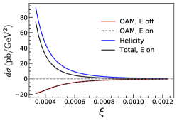
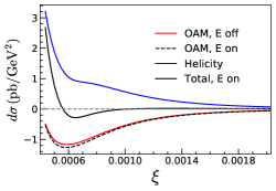
Figure 5: The DSA part of the differential cross-section, both with and without $E_{g}$, is presented as a function of $\xi$ at $Q^{2}=2.7\,\textrm{GeV}^{2}$ (left), $Q^{2}=4.8\,\textrm{GeV}^{2}$ (middle), and $Q^{2}=10\,\textrm{GeV}^{2}$ (right). The results with $E_{g}=0$ correspond to those reported in our previous work Bhattacharya et al. (2022a). These plots suggest that the incorporation of contributions from $E_{g}$ into the orbital angular momentum does not result in a significant alteration of our previous results.

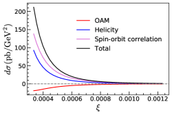
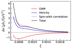
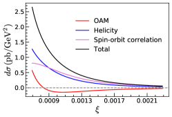
Figure 6: The DSA part of the differential cross-section with $E_{g}\neq 0$ is presented as a function of $\xi$ at $Q^{2}=2.7\,\textrm{GeV}^{2}$ (left), $Q^{2}=4.8\,\textrm{GeV}^{2}$ (middle), and $Q^{2}=10\,\textrm{GeV}^{2}$ (right). These plots include contributions from spin-orbit correlation, explicitly demonstrating how the results in the above figure are quantitatively modified in the presence of this contribution.

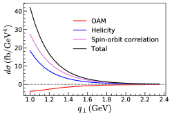
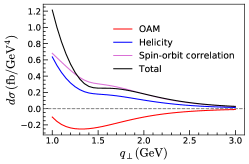
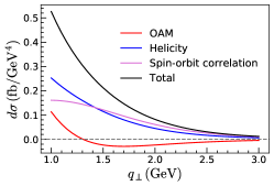
Figure 7: The DSA part of the differential cross-section with $E_{g}\neq 0$ is presented as a function of $q_{\perp}$ at $Q^{2}=2.7\,\textrm{GeV}^{2}$ (left), $Q^{2}=4.8\,\textrm{GeV}^{2}$ (middle), and $Q^{2}=10\,\textrm{GeV}^{2}$ (right).

In Fig. 5 and Fig. 6, we present Eq. (217) as functions of $\xi$. In the former, we display the results of our previous work with $E_{g}$ activated, contrasting them with our published findings. In the latter, we introduce the spin-orbit correlation term. Our analysis reveals that the OAM and helicity contributions tend to either cancel or reinforce each other, depending on $Q^{2}$, as discussed earlier. Notably, the spin-orbit correlation and helicity terms exhibit comparable magnitudes and are substantial. Since the spin-orbit correlation is solely dictated by the unpolarized gluon distribution, it is relatively better constrained than OAM, which requires precise knowledge of both unpolarized and polarized gluon distributions. The latter has significant uncertainties, particularly at small $x$. Subtracting the contributions from the helicity and spin-orbit correlation terms could provide direct sensitivity to OAM.

In Fig. 7, we present the same plot as in Fig. 6, but now as a function of the dijet transverse momentum $q_{\perp}$. Note that the units of the vertical axis have changed pb $\to$ fb (apart from the trivial dimensional factor GeV^-2). This is because of the typical value $\xi\sim 10^{-3}$ probed in this kinematics.

It is important to emphasize that our numerical estimations incorporated several approximations, including systematic errors inherent in the double distribution method and the Wandzura-Wilczek approximation. However, the primary source of uncertainty lies in the unpolarized and especially polarized gluon distributions which are currently not well constrained at small-$x$. Moreover, ideally the next-to-leading order corrections should be included Boussarie et al. (2016). Due to these reasons, we did not attempt to include error bars in the above plots. Therefore, our numerical results provide only a rough estimate of the overall magnitudes and signs of various contributions. In the future, as more accurate determinations of $\Delta G(x)$ become available, our predictions can be correspondingly improved.

VI.3 Results for SIDDIS process

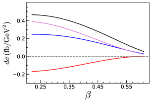
Figure 8: Plot depicting the SIDDIS cross section as a function of the $\beta$ parameter for $\Lambda=1$ GeV and at two different $Q^{2}$ values: $2.7\,\textrm{GeV}^{2}$ (left) and $10\,\textrm{GeV}^{2}$ (right). The maximum $\beta$ value is restricted by the condition $q_{\perp}<1$ GeV.

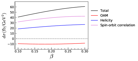
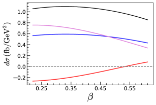
Figure 9: Plot depicting the SIDDIS cross section as a function of the $\beta$ parameter for $\Lambda=0.5$ GeV and at two different $Q^{2}$ values: $2.7\,\textrm{GeV}^{2}$ (left) and $10\,\textrm{GeV}^{2}$ (right). The change of OAM sign, resulting from the interplay between OAM and helicity at small $x$, is once again clearly observable in the high $\beta$ region.

In Figs. 8 and 9, we present the SIDDIS cross section as a function of the $\beta$ parameter for two distinct cutoff values: $\Lambda=1.0$ and $0.5$ GeV. The calculation considers tagged hadron species, such as charged pions and kaons, while the fragmentation quarks are assumed to be $u,\bar{u},d,\bar{d},s$ and $\bar{s}$. The change in the sign mechanism of the OAM, as observed in the dijet process, is also evident here for $\Lambda=0.5$ GeV and in the higher regions of $\beta$. While the obtained number values suggest that measuring this process might still be challenging, our main point is that there is no need to reconstruct the dijet transverse momentum, yet sensitivity to OAM is retained. Therefore, this approach may offer a promising route for measurement at the EIC to constrain OAM.

VII Conclusion

In conclusion, our overarching goal has been to identify and establish ‘practical’ physical observables capable of directly measuring parton orbital angular momentum (OAM). In this endeavor, we have expanded upon our previous work Bhattacharya et al. (2022a) by offering a comprehensive analysis of the longitudinal double spin asymmetry in exclusive dijet production during electron-proton scattering. Our investigation reaffirms the sensitivity of the $\cos\phi$ angular correlation as a crucial indicator of gluon OAM at small-$x$, and its intricate interplay with gluon helicity. Furthermore, our study uncovers an additional aspect unexplored in our prior research: the spin-orbit correlation of gluons $C_{g}(x)$. For the first time, we shed light on the small-$x$ behavior of this distribution (see also S. Bhattacharya, R. Boussarie, and Y. Hatta (2024)) and find that it is approximately proportional to the unpolarized gluon distribution but with an opposite sign. Consequently, its contribution to the present observable is unsuppressed, contrary to naive expectations. The determination of OAM therefore necessitates accurate knowledge of the unpolarized gluon distribution at small-$x$, in addition to the polarized gluon distribution $\Delta G(x)$. Alternatively, since the spin-orbit correlation exists already in unpolarized hadrons, one may be able to constrain $C_{g}(x)$ (including the genuine twist-three contributions) from other spin-independent exclusive processes, see, e.g., Boussarie et al. (2018). Based on the analytical results, we have performed a detailed numerical analysis in both dijet and semi-inclusive diffractive deep inelastic scattering processes. The latter may offer experimental advantages as it does not require the reconstruction of dijet transverse momenta; instead, it involves the inclusive tagging of one or more hadron species.

We have also undertaken the first exploration of quark-channel contributions to double spin asymmetry, revealing an unexpected breakdown of factorization. Indeed, even in the gluon case, we encountered an ‘end-point’ singularity at $x=\pm\xi$ which we circumvented by restricting to $z\sim 1/2$. In the quark case, we observed a similar singularity across all $z$ values due to the $C$-odd exchange in the $t$-channel. We recognize the importance of revisiting the present calculation using a dedicated $k_{T}$ factorization approach. This approach holds promise to remedy the problems with factorization and make the amplitude manifestly finite. But the connection to parton OAMs becomes necessarily less direct.

Overall, our work contributes significantly to the ongoing efforts aimed at unraveling the orbital angular momentum of partons and its role in shaping the spin structure of the nucleon. We anticipate that our findings will serve as a valuable foundation for inspiring and guiding further studies in this field.

Appendix A Compton form factors

In this appendix we collect formulas for the Compton form factors introduced in (120), (131) and (155) that are useful for the numerical evaluation of (164).

$${\cal H}^{(1)}_{g}(\xi) =\frac{1}{\xi}\left(H_{g}(\xi,\xi)\ln\frac{1-\xi}{1+\xi}+\int_{-1}^{1}dx\frac{H_{g}(x,\xi)-H_{g}(\xi,\xi)}{x-\xi}\right)-i\dfrac{\pi}{\xi}H_{g}(\xi,\xi),$$ (218)

$${\cal H}^{(2)}_{g}(\xi) =\dfrac{1}{2}\bigg{(}H^{\prime}_{g}(\xi,\xi)\ln\dfrac{1-\xi}{1+\xi}+\int_{-1}^{1}dx\frac{H^{\prime}_{g}(x,\xi)-H^{\prime}_{g}(\xi,\xi)}{x-\xi}\bigg{)}$$

$$-\dfrac{1}{2\xi}\left(H_{g}(\xi,\xi)\ln\frac{1-\xi}{1+\xi}+\int_{-1}^{1}dx\frac{H_{g}(x,\xi)-H_{g}(\xi,\xi)}{x-\xi}\right)-i\frac{\pi}{2}\bigg{(}H^{\prime}_{g}(\xi,\xi)-\dfrac{1}{\xi}H_{g}(\xi,\xi)\bigg{)},$$ (219)

$$\tilde{\cal H}^{(2)}_{g}(\xi) =\dfrac{1}{2}\bigg{(}\tilde{H}^{\prime}_{g}(\xi,\xi)\ln\dfrac{1-\xi}{1+\xi}+\int_{-1}^{1}dx\frac{\tilde{H}^{\prime}_{g}(x,\xi)-\tilde{H}^{\prime}_{g}(\xi,\xi)}{x-\xi}\bigg{)}-i\frac{\pi}{2\xi}\tilde{H}^{\prime}_{g}(\xi,\xi),$$ (220)

$${\cal L}^{(2)}_{g}(\xi) =\frac{1}{2\xi}\bigg{(}Y_{g}(\xi,\xi)\ln\frac{1-\xi}{1+\xi}+\int_{-1}^{1}dx\frac{Y_{g}(x,\xi)-Y_{g}(\xi,\xi)}{x-\xi}\bigg{)}-i\dfrac{\pi}{2\xi}Y_{g}(\xi,\xi),$$ (221)

where we defined $H^{\prime}_{g}(x,\xi)\equiv\dfrac{d}{dx}{H_{g}(x,\xi)}$, $\tilde{H}^{\prime}_{g}(x,\xi)\equiv\dfrac{d}{dx}{\tilde{H}_{g}(x,\xi)}$, and $Y_{g}(x,\xi)\equiv\dfrac{d}{dx}xL_{g}(x,\xi)$. $C_{g}^{(2)}(\xi)$ is obtained via the same formula as (219) with $H_{g}(x,\xi)\to xC_{g}(x,\xi)$.

Note that, when $\xi\ll 1$, ${\cal H}_{g}^{(1,2)}$ are dominated by the imaginary parts

$${\mathfrak{I}m}{\cal H}_{g}^{(1)}(\xi)=-\frac{\pi}{\xi}H_{g}(\xi,\xi),\qquad{\mathfrak{I}m}{\cal H}^{(2)}_{g}(\xi)=-\frac{\pi}{2}\left(\left.\frac{dH_{g}(x,\xi)}{dx}\right|_{x=\xi}-\frac{1}{\xi}H_{g}(\xi,\xi)\right).$$ (222)

Moreover, assuming a Regge-like behavior $H_{g}(x,\xi)\sim\frac{1}{x^{c}}$ with $c\propto\alpha_{s}$, we see that the second term in ${\cal H}_{g}^{(2)}$ is parametrically larger than the first term. This leads to the relation

$${\rm Im}{\cal H}_{g}^{(1)}(\xi)\approx-2{\rm Im}{\cal H}_{g}^{(2)}(\xi).$$ (223)

In Figs. 10, 11, and 12 we present plots depicting both the real and imaginary components of the Compton form factors as functions of $\xi$. As anticipated, the imaginary components of the Compton factors ${\cal{H}}^{(1,2)}_{g}$ significantly outweigh their real counterparts at small $\xi$ values. We also see that the relation (223) is approximately satisfied. However, these properties do not hold for the helicity and OAM Compton factors ${\cal{\tilde{H}}}^{(2)}_{g}$ and ${\cal L}_{g}^{(2)}$. From the plots, we observe that the real parts are nearly as prominent as the imaginary ones for small $\xi$ values and they roughly satisfy

$$\tilde{\cal H}_{g}^{(2)}\approx-{\cal L}_{g}^{(2)},$$ (224)

as expected (see a comment after (165)). Somewhat unexpectedly, however, we find that $|\tilde{\cal H}_{g}^{(2)}|\sim|{\cal L}_{g}^{(2)}|$ are about an order of magnitude larger than $|{\cal H}_{g}^{(1,2)}|$, cf., a comment below (17).

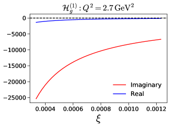
Figure 10: CFFs of the unpolarized gluon GPDs.

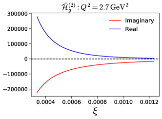
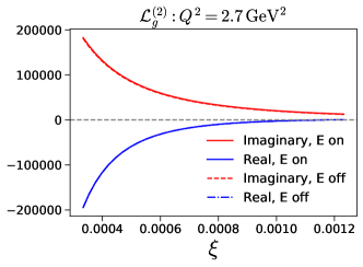
Figure 11: CFFs of the helicity (left) and OAM (right) distributions.

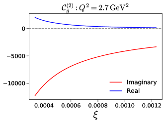
Figure 12: CFFs of the spin-orbit correlation.

References

- Bhattacharya et al. (2022a) S. Bhattacharya, R. Boussarie, and Y. Hatta, Phys. Rev. Lett. 128, 182002 (2022a), eprint 2201.08709.
- Jaffe and Manohar (1990) R. L. Jaffe and A. Manohar, Nucl. Phys. B 337, 509 (1990).
- Adamczyk et al. (2015) L. Adamczyk et al. (STAR), Phys. Rev. Lett. 115, 092002 (2015), eprint 1405.5134.
- de Florian et al. (2014) D. de Florian, R. Sassot, M. Stratmann, and W. Vogelsang, Phys. Rev. Lett. 113, 012001 (2014), eprint 1404.4293.
- Nocera et al. (2014) E. R. Nocera, R. D. Ball, S. Forte, G. Ridolfi, and J. Rojo (NNPDF), Nucl. Phys. B 887, 276 (2014), eprint 1406.5539.
- Abdallah et al. (2022) M. S. Abdallah et al. (STAR), Phys. Rev. D 105, 092011 (2022), eprint 2110.11020.
- Abdul Khalek et al. (2022) R. Abdul Khalek et al., Nucl. Phys. A 1026, 122447 (2022), eprint 2103.05419.
- Lorce and Pasquini (2011) C. Lorce and B. Pasquini, Phys. Rev. D 84, 014015 (2011), eprint 1106.0139.
- Hatta (2012) Y. Hatta, Phys. Lett. B 708, 186 (2012), eprint 1111.3547.
- Lorce et al. (2012) C. Lorce, B. Pasquini, X. Xiong, and F. Yuan, Phys. Rev. D 85, 114006 (2012), eprint 1111.4827.
- Hatta and Yoshida (2012) Y. Hatta and S. Yoshida, JHEP 10, 080 (2012), eprint 1207.5332.
- Ji et al. (2013) X. Ji, X. Xiong, and F. Yuan, Phys. Rev. D 88, 014041 (2013), eprint 1207.5221.
- Rajan et al. (2016) A. Rajan, A. Courtoy, M. Engelhardt, and S. Liuti, Phys. Rev. D 94, 034041 (2016), eprint 1601.06117.
- Engelhardt (2017) M. Engelhardt, Phys. Rev. D 95, 094505 (2017), eprint 1701.01536.
- Boussarie et al. (2019) R. Boussarie, Y. Hatta, and F. Yuan, Phys. Lett. B 797, 134817 (2019), eprint 1904.02693.
- Guo et al. (2021) Y. Guo, X. Ji, and K. Shiells, Nucl. Phys. B 969, 115440 (2021), eprint 2101.05243.
- Kovchegov (2019) Y. V. Kovchegov, JHEP 03, 174 (2019), eprint 1901.07453.
- Engelhardt et al. (2020) M. Engelhardt, J. R. Green, N. Hasan, S. Krieg, S. Meinel, J. Negele, A. Pochinsky, and S. Syritsyn, Phys. Rev. D 102, 074505 (2020), eprint 2008.03660.
- Kovchegov and Manley (2024) Y. V. Kovchegov and B. Manley, JHEP 02, 060 (2024), eprint 2310.18404.
- Manley (2024) B. Manley (2024), eprint 2401.05508.
- Ji et al. (2017) X. Ji, F. Yuan, and Y. Zhao, Phys. Rev. Lett. 118, 192004 (2017), eprint 1612.02438.
- Hatta et al. (2017) Y. Hatta, Y. Nakagawa, F. Yuan, Y. Zhao, and B. Xiao, Phys. Rev. D 95, 114032 (2017), eprint 1612.02445.
- Bhattacharya et al. (2017) S. Bhattacharya, A. Metz, and J. Zhou, Phys. Lett. B 771, 396 (2017), [Erratum: Phys.Lett.B 810, 135866 (2020)], eprint 1702.04387.
- Bhattacharya et al. (2022b) S. Bhattacharya, A. Metz, V. K. Ojha, J.-Y. Tsai, and J. Zhou, Phys. Lett. B 833, 137383 (2022b), eprint 1802.10550.
- Boussarie et al. (2018) R. Boussarie, Y. Hatta, B.-W. Xiao, and F. Yuan, Phys. Rev. D 98, 074015 (2018), eprint 1807.08697.
- Courtoy et al. (2014) A. Courtoy, G. R. Goldstein, J. O. Gonzalez Hernandez, S. Liuti, and A. Rajan, Phys. Lett. B 731, 141 (2014), eprint 1310.5157.
- Bhattacharya et al. (2023a) S. Bhattacharya, D. Zheng, and J. Zhou (2023a), eprint 2304.05784.
- Bhattacharya et al. (2023b) S. Bhattacharya, D. Zheng, and J. Zhou (2023b), eprint 2312.01309.
- Hatta et al. (2022) Y. Hatta, B.-W. Xiao, and F. Yuan, Phys. Rev. D 106, 094015 (2022), eprint 2205.08060.
- Meissner et al. (2009) S. Meissner, A. Metz, and M. Schlegel, JHEP 08, 056 (2009), eprint 0906.5323.
- Bomhof et al. (2006) C. J. Bomhof, P. J. Mulders, and F. Pijlman, Eur. Phys. J. C 47, 147 (2006), eprint hep-ph/0601171.
- Dominguez et al. (2011) F. Dominguez, C. Marquet, B.-W. Xiao, and F. Yuan, Phys. Rev. D 83, 105005 (2011), eprint 1101.0715.
- Altinoluk et al. (2016) T. Altinoluk, N. Armesto, G. Beuf, and A. H. Rezaeian, Phys. Lett. B 758, 373 (2016), eprint 1511.07452.
- Hatta et al. (2016) Y. Hatta, B.-W. Xiao, and F. Yuan, Phys. Rev. Lett. 116, 202301 (2016), eprint 1601.01585.
- Boussarie et al. (2016) R. Boussarie, A. V. Grabovsky, L. Szymanowski, and S. Wallon, JHEP 11, 149 (2016), eprint 1606.00419.
- Hatta and Yao (2019) Y. Hatta and X. Yao, Phys. Lett. B 798, 134941 (2019), eprint 1906.07744.
- Hatta and Zhou (2022) Y. Hatta and J. Zhou, Phys. Rev. Lett. 129, 252002 (2022), eprint 2207.03378.
- Kuraev et al. (1977) E. A. Kuraev, L. N. Lipatov, and V. S. Fadin, Sov. Phys. JETP 45, 199 (1977).
- Balitsky and Lipatov (1978) I. I. Balitsky and L. N. Lipatov, Sov. J. Nucl. Phys. 28, 822 (1978).
- Bartels et al. (1996a) J. Bartels, B. I. Ermolaev, and M. G. Ryskin, Z. Phys. C 72, 627 (1996a), eprint hep-ph/9603204.
- Borden and Kovchegov (2023) J. Borden and Y. V. Kovchegov, Phys. Rev. D 108, 014001 (2023), eprint 2304.06161.
- More et al. (2018) J. More, A. Mukherjee, and S. Nair, Eur. Phys. J. C 78, 389 (2018), eprint 1709.00943.
- Hatta and Yang (2018) Y. Hatta and D.-J. Yang, Phys. Lett. B 781, 213 (2018), eprint 1802.02716.
- Braun and Ivanov (2005) V. M. Braun and D. Y. Ivanov, Phys. Rev. D 72, 034016 (2005), eprint hep-ph/0505263.
- Zhou (2014) J. Zhou, Phys. Rev. D 89, 074050 (2014), eprint 1308.5912.
- Szymanowski and Zhou (2016) L. Szymanowski and J. Zhou, Phys. Lett. B 760, 249 (2016), eprint 1604.03207.
- Ji (1992) X.-D. Ji, Phys. Lett. B 289, 137 (1992).
- Agrawal et al. (2023) S. Agrawal, N. Vasim, and R. Abir (2023), eprint 2312.04132.
- Boer et al. (2018) D. Boer, T. Van Daal, P. J. Mulders, and E. Petreska, JHEP 07, 140 (2018), eprint 1805.05219.
- S. Bhattacharya, R. Boussarie, and Y. Hatta (2024) S. Bhattacharya, R. Boussarie, and Y. Hatta (2024), eprint 2404.xxxxx.
- Cui et al. (2019) Z. L. Cui, M. C. Hu, and J. P. Ma, Eur. Phys. J. C 79, 812 (2019), eprint 1804.05293.
- Anikin et al. (2000) I. V. Anikin, B. Pire, and O. V. Teryaev, Phys. Rev. D 62, 071501 (2000), eprint hep-ph/0003203.
- Diehl (2003) M. Diehl, Phys. Rept. 388, 41 (2003), eprint hep-ph/0307382.
- Mankiewicz and Piller (2000) L. Mankiewicz and G. Piller, Phys. Rev. D 61, 074013 (2000), eprint hep-ph/9905287.
- Anikin and Teryaev (2003) I. V. Anikin and O. V. Teryaev, Phys. Lett. B 554, 51 (2003), eprint hep-ph/0211028.
- Nabeebaccus et al. (2023) S. Nabeebaccus, J. Schoenleber, L. Szymanowski, and S. Wallon (2023), eprint 2311.09146.
- Reinke Pelicer et al. (2019) M. Reinke Pelicer, E. Gräve De Oliveira, and R. Pasechnik, Phys. Rev. D 99, 034016 (2019), eprint 1811.12888.
- Bergabo and Jalilian-Marian (2022) F. Bergabo and J. Jalilian-Marian, Phys. Rev. D 106, 054035 (2022), eprint 2207.03606.
- Linek et al. (2023) B. Linek, A. Łuszczak, M. Łuszczak, R. Pasechnik, W. Schäfer, and A. Szczurek (2023), eprint 2308.00457.
- Fucilla et al. (2023) M. Fucilla, A. V. Grabovsky, E. Li, L. Szymanowski, and S. Wallon, JHEP 03, 159 (2023), eprint 2211.05774.
- Bartels et al. (1996b) J. Bartels, H. Lotter, and M. Wüsthoff, Phys. Lett. B 379, 239 (1996b), [Erratum: Phys.Lett.B 382, 449–449 (1996)], eprint hep-ph/9602363.
- Forshaw and Ross (1998) J. R. Forshaw and D. A. Ross, Quantum Chromodynamics and the Pomeron, vol. 9 (Oxford University Press, 1998), ISBN 978-1-00-929011-1, 978-1-00-929010-4, 978-1-00-929012-8, 978-0-511-89326-1, 978-0-521-56880-7.
- Fucilla et al. (2024) M. Fucilla, A. Grabovsky, E. Li, L. Szymanowski, and S. Wallon, JHEP 02, 165 (2024), eprint 2310.11066.
- Guo and Yuan (2023) Y. Guo and F. Yuan (2023), eprint 2312.01008.
- Radyushkin (1999) A. V. Radyushkin, Phys. Rev. D 59, 014030 (1999), eprint hep-ph/9805342.
- Radyushkin (2000) A. V. Radyushkin (2000), eprint hep-ph/0101225.
- Sato et al. (2020) N. Sato, C. Andres, J. J. Ethier, and W. Melnitchouk (JAM), Phys. Rev. D 101, 074020 (2020), eprint 1905.03788.
- Ethier et al. (2017) J. J. Ethier, N. Sato, and W. Melnitchouk, Phys. Rev. Lett. 119, 132001 (2017), eprint 1705.05889.
- Tan and Lu (2023) C. Tan and Z. Lu, Phys. Rev. D 108, 054038 (2023), eprint 2301.09081.