An Insight of Heart-Like Systems with Percolation

Abstract

We study the signal percolation through heart-like biological system. Starting from an initial distribution of Waiting and Inactive cells with probabilities $p$ and $(1-p)$ respectively the signal propagation is observed in terms of Active cells. As the signal enters the system from one end, the number of arrival of Active sites at the other end is studied and analysis of the system behaviour is made by varying a few important parameters of the system like $p_{switch}$ (switching probability from Inactive to Waiting) and $p_{act}$ (switching probability from Waiting to active). In this connection, the non-regular heart rhythms are discussed. Fraction of percolating paths through the system is studied and showed a transition from $0$ to $1$ near $p=p_{c}$. Some other important quantities like tortuosity and cluster distribution are discussed and corresponding exponents have been found.

Introduction

Percolation is one of the simplest and fundamental models in statistical mechanics which is not always an exactly solvable model. In spite of its simple update rules, it can be applied to describe a wide variety of systems. Not only for the study of the dynamics of fluids through porous media [1] but it can as well be applied to study the electrical movement in neurons, fibrosis in organs, damage spreading in solids through fiber bundle model, disease spreading in a community, opinion formation in society or even for knowledge percolation [2, 3, 4, 5, 6, 7, 8, 9].

A very popular model of Percolation is the forest fire model (FFM) introduced in [10, 11] mainly as a 2D lattice. There are several variations of the model [11, 12]. In one, the fire can spread from top to bottom and from left to right can be regarded as a general “Directed Percolation” (DP) model. For DP, it is well understood that the bottom to top and right to left movements are prohibited [13, 14]. There are other models of percolation where all top to bottom, bottom to top, left to right and right to left movements are all allowed and can be termed as Isotropic Percolation (IP). However, the model where the percolation is allowed in the top to bottom direction and sideways can be termed as Semi Directed Percolation (SDP). This was introduced for the first time [15] in a random resistor-diode network in [16]. It has also been studied in square and triangular lattices [17]. However in both [16, 17], it was termed not as SDP but as Partially Directed Percolation.

The movement of signal in neurons for the heart and brain systems [2, 3, 4, 5] can be studied in the light of percolation. Movement of heat and electrical signal through different media have been studied in [19, 18] by percolation methods. In addition to this, there are certain important quantities like ‘Tortuosity’ which have been studied for a few systems in combination with percolation [20].

This process of signal percolation through heart is an interesting topic to study. When the heartbeats do not follow the usual pattern but become very fast or irregular, it leads to a disease called arrhythmia [21]. Arrhythmias in turn cause health situations such as fainting, stroke, heart attack or even death. Normally, a special group of cells in the sinoatrial (SA) node in the upper right chamber of the heart begin the electrical signal to start the heartbeat. This signal travels down the heart towards the ventricles, i.e., the two lower chambers of the heart. This organized pattern helps the heart to beat in its usual way. However, several problems affect the normal conduction of signal and lead to abnormal heart rhythms. Due to faster beats, there may not be enough time in between beats and this may prevent the heart from pumping the required amount of blood to the whole body which may lead to arrhythmia and related health problems.

Several biological models have been used to study the heart system with the help of computation. Computational models in cardiology showed enormous scope in revealing diagnostic information related to cardiac disease. At the same time there is provisions that these models help the diagnosis to be cost-effective and to have low risk [5]. The cells can be activated by an external stimulus which initiates an Action Potential (AP). The cells after activation will go through a certain refractory period. The exact physiological processes are described in [22] in a detailed manner. In [6], the model of heart is studied with three states of cells: active, inactive and waiting in connection with the AP.

One of the simplified system to study a percolation problem is a $L\times L$ lattice, where there is a parameter called percolation probability $p$ with which a site could be open, i.e. can percolate “something”. This in turn indicates that a site is closed with $1-p$ probability, means unable to percolate. It is well known from different studies that below a critical percolation probability $p_{c}$ the system is unable to percolate, whereas above $p_{c}$ infinite percolation cluster can be formed. In connection to percolation there are a number of exponents which can be studied as well. Those exponents actually describes the system near criticality.

Description of the Model

We study a 2D square grid of $L\times L$ cells where initially the cells may be in two states, “Waiting” and “Inactive” as described in [6] also. A “Waiting” cell is an open cell which is ready to hold anything percolating through the system. An “Inactive” cell is however equivalent to a closed cell which is unable to percolate. We choose the system with an initial distribution of “Waiting” cells with probability $p$ and “Inactive” cells with probability $1-p$. A “Waiting” cell can be activated with an action potential (the thing that is actually percolating through the system) and then it becomes an “Active” one. The condition for a Waiting cell to transform into an Active one in the next step is that one or more of its “nearest cell neighbors” should be Active. An “Active” cell which is holding the Action Potential at a particular instant will be transformed into an “Inactive” one in the next time step. For a heart system this is consistent with the fact that there is a certain refractory period of the cells.

From now on, we will use numbers to indicate the type of the cells for our convenience. Thus

• an “Waiting” cell will be identified as “$0$”,

• an “Active” cell will be identified as “$1$”,

• an “Inactive” cell will be identified as “$2$”.

The general rule of transformation for a cell may be described as: Waiting $\rightarrow$ Active $\rightarrow$ Inactive, or, using the numbers as $0\rightarrow 1\rightarrow 2$. However, in some specific cases an “Inactive” cell may become a “Waiting” one, i.e., $2\rightarrow 0$ is also allowed. This is similar to the tree regrowth at several sites in Forest Fire Model as discussed in [10, 11].

In addition to these rules, some definite probabilities are considered to be associated with this system. We introduce two probabilities:

• $p_{act}$(inhibitory) by which an Waiting cell can become an Active one, i.e., $0\rightarrow 1$.

• $p_{switch}$(refractory) by which an Inactive cell can be reverted to a Waiting one, i.e., $2\rightarrow 0$.

.

The AP is initiated from one side (here from the top) of the 2D matrix. This is done by labelling all the cells on the first row as $1$. The different rows are updated at different times $t$. It is obvious that to receive the AP at the bottom/final row the number of time steps required will at least be equal to the system size $L$.

The system is studied from two aspects. First, the number of arrival $N_{A}$ at the other end of the 2D matrix is observed with variation of the parameters $p_{act}$ and $p_{switch}$ in subsection A of the Results. If there is no Inactive cell, the AP reach all the cells of the final row in time $L$. However, when there is a distribution of $0$ and $2$ cells, all the cells of the final row do not contain the AP at the same time but $1$s arrive at different cells at different times. At the final row the number of cells containing the AP is counted at each time. Second, the percolation model of the system is analyzed. The delay in arrival is measured and some interesting properties related to that are studied. In the same context the cluster distribution and several exponents related to the system are also studied. The corresponding results are shown in subsections B and C of the Results.

Results

.1 Study of Number of Arrival

The Action Potential as initiated from one end of the 2D lattice of size $L$ percolates through the system. The number of arrivals at the other end, i.e., the active sites at that ends $N_{A}$ is checked with time $t$ . We will study the number of arrivals $N_{A}$ with two conditions:

1. When the $2\rightarrow 0$ transition is not allowed $p_{switch}=0.0$ : This arises when the cells after becoming Active receiving the AP for once become inactive and stay in their refractory period for a very long time. Here $p_{switch}=0.0$ is equivalent to an infinite refractory period. This can be often seen due to certain health condition. For old people this is very common [23]. At the same time it may also happen that the transition from $0\rightarrow 1$ can occur with probability less than $1$. This may also happen due to some irregularity in the cell activation [24].

2. When $2\rightarrow 0$ transition is allowed with a certain probability other than $0.0$ : Here $p_{switch}\neq 0.0$ indicates that the cells are in their refractory period. However, very small value of $p_{switch}$ indicates that the cells are in their refractory period for longer than usual. Medications and better lifestyle may lead the system to have a higher $p_{switch}$. However, having a very larger value of $p_{switch}$ is not suitable for this case and will be discussed later.

In addition to $p_{switch}=0.0$ there may be variation of $p_{act}$ with which we have studied the system.

The variation of number of arrival $N_{A}$ with $t$ is shown in Fig. 1 for $p_{act}=1$ and $p_{switch}$ varying from $0.0$ to $0.9$. The plots show some kind of oscillatory behaviour for high values of $p_{switch}$ and finally saturate to some specific non-zero values $(N_{A})_{sat}$.

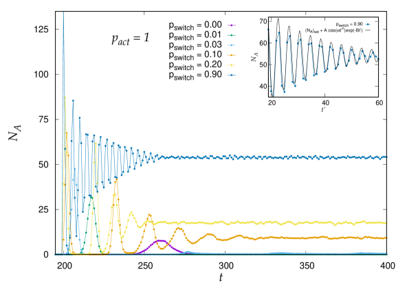
Figure 1: $N_{A}$ vs $t$ with $L$ = 200, $p=0.70$, $p_{act}=1.0$ and $p_{switch}$ varying from $0$ to $0.90$. In the inset $p_{switch}=0.90$ has been shown with equation 3 where $(N_{A})_{sat}\simeq 54$, $A=55$ and $B=0.05$.

The oscillatory behaviour can be explained in the following way. It is well known that when a fluid is flowing through a porous medium, there is some kind of relative motion [25] which generates a fluid shear [19], can be considered as a friction/damping. In the same way, when an electrical signal, here the AP, is moving through the heart, there must be some retardation present. For high $p_{switch}$, the motion is similar to an underdamped oscillatory one. This is obvious as for high $p_{switch}$, the signal more frequently finds a path to percolate, be it in forward or backward directions or sideways. Therefore number of arrival $N_{A}$ is never zero. However, for $p_{switch}=0.0$, it has been observed that the behaviour of $N_{A}$ is Gaussian. This signifies that for low $p_{switch}$ the number of active cells die down almost completely in time $L<t<2L$. Therefore for further AP signals there is no chance to pass down through the system. However, for higher $p_{switch}$, this is not true and even after a very long time there is always a chance for the next APs to pass through the system. This is because here we have $(N_{A})_{sat}>0$ always that indicateds a certain finite number of Active cells will always be present in the system. Even if we study the system for $t\rightarrow\infty$ the system still shows non-zero active sites.

It is already observed that for $p_{switch}\rightarrow 1$ the system shows a damped oscillatory behaviour. Therefore it is worth comparing the system parameters to the parameters associated with a damped oscillator. The differential equation of a damped oscillator is

$$\frac{d^{2}x}{dt^{2}}+2B\frac{dx}{dt}+\omega_{0}^{2}x=0$$ (1)

where the coefficient $2B$ is related to damping and $\omega_{0}$ is the natural frequency of oscillation. For underdamped/oscillatory motion $B^{2}<\omega_{0}^{2}$ and the corresponding solution can be written as

$$x(t)=A\cos(\omega t)\exp(-Bt)$$ (2)

where $\omega=\sqrt{\omega_{0}^{2}-B^{2}}$. For this purpose, we fit $N_{A}$ with the following function:

$$N_{A}(t)=(N_{A})_{sat}+A\cos(\omega{t^{\prime}}^{\nu})\exp(-Bt^{\prime})$$ (3)

where $t^{\prime}=t-L$. The approximate values are shown in Table 1.

$p_{switch}$	$(N_{A})_{sat}$	$A$	$\omega$	$\nu$	$B$
0.90	53.83	55	1.00	1.10	0.05
0.80	48.78	58	0.65	1.20	0.07
0.70	45.31	70	0.45	1.29	0.09
0.60	41.21	75	0.31	1.37	0.10

Table 1: Approximate values of the parameters in Equation 3 with $L=200$.

In case of $p_{act}=p_{switch}=1$ (not shown in Fig. 1) the oscillatory behaviour continues as the rows are updating as waiting $\rightarrow$ active $\rightarrow$ inactive $\rightarrow$ waiting.

We now fix $p_{switch}=0$ and study the system behaviour by varying $p_{act}$. It is already clear from Fig. 1 that the behaviour will be approximately Gaussian. In Fig. 2 the behaviour is shown for $0.85\leqslant p_{act}\leqslant 1.0$. The parameters related to the Gaussian behaviour is shown in Table 2 for $L=200$ by fitting with the following function:

$$N_{A}(t)=(N_{A})_{max}e^{-\frac{1}{2}\left(\frac{t-\mu}{\sigma_{sd}}\right)^{2}}.$$ (4)

where $(N_{A})_{max}$ is the peak value, $\mu$ is the mean and $\sigma_{sd}$ is the standard deviation of the Gaussian profile.

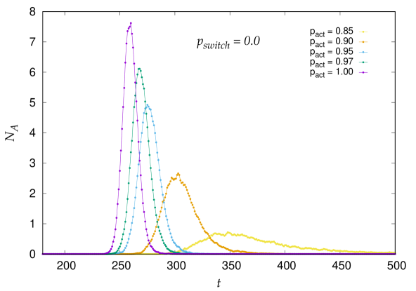
Figure 2: $N_{A}$ vs $t$ with $L=200$, $p_{switch}=1.0$ and $p_{act}$ varies from $0.85$ to $1.00$.

$p_{act}$	$(N_{A})_{max}$	$\mu$	$\sigma_{sd}$
$1.00$	$7.78$	$259.10$	$6.35$
$0.97$	$6.20$	$268.32$	$7.48$
$0.95$	$4.89$	$275.54$	$9.22$
$0.90$	$2.66$	$303.00$	$14.01$
$0.85$	$0.66$	$356.50$	$33.71$

Table 2: Approximate values of the parameters in Equation 4 with $L=200$.

It is observed that as $p_{act}$ decreases, $(N_{A})_{max}$ decreases. It is in agreement to our description of the model. For $p_{act}<1$ the Waiting cells do not receive the AP with $100\%$ probability and therefore cannot become Active. Therefore $(N_{A})_{max}$ decreases. The movement of the peak towards right with decreasing $p_{act}$, i.e., shifting of the mean of the Gaussian profile towards higher $t$ can also be explained in the following manner: As $p_{act}<1$ the signal cannot find its way smoothly inside the system and therefore must take a longer time to appear at the other end. The variations of $(N_{A})_{max}$, $\mu$ and $\sigma_{sd}$ are shown as a function of $p_{act}$ in Fig, 3 for $L=50,100,200$.

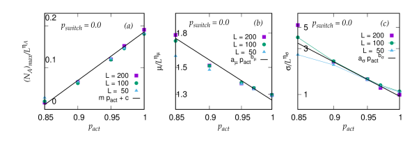
Figure 3: Variations of the Gaussian parameters with $p_{act}$ where $L=50,100$ and $200$, (a) $\frac{(N_{A})_{max}}{L^{\eta_{A}}}$ versus $p_{act}$ with $\eta_{A}=0.7$, $m=1.16\pm 0.05$ and $c=-0.98\pm 0.05$, (b) $\frac{\mu}{L^{\eta_{\mu}}}$ versus $p_{act}$ with $\eta_{\mu}=1.0$, $a_{\mu}=1.26\pm 0.03$ and $b_{\mu}=-2.02\pm 0.20$ and (c) $\frac{\sigma}{L^{\eta_{\sigma}}}$ vs $p_{act}$ with $\eta_{\sigma}=1.0$, $a_{\sigma}=0.96\pm 0.03$ and $b_{\mu}=-7.82\pm 0.36$.

From Fig. 2 it is evident that with decrease of $p_{act}$ the curve broadens and the height of the peak decreases. This suggests that not only arrivals are delayed because of obstacles within the system, the signal is getting weakened too. If we analyze the area under the curve carefully, it is evident that it is decreasing with decrease in $p_{act}$. This also confirms presence of some kind of retardation as it usually present for a real heart system.

.2 Study of Percolating Paths and Tortuosity

Next we study the probability $P_{N}$ in terms of the fraction of percolating paths out of a $N_{T}$ number of trials against $p$. This is shown in Fig. 4 for $p_{act}=1.0,p_{switch}=0.0$ for different $L$. Here we have taken $N_{T}=1000$. In the inset of Fig. 4 the data collapse has been shown. It has been observed that the percolation threshold is at $p_{c}\simeq 0.59$ which is in good agreement with [26, 27, 28, 29]. The function is checked to be fitted with the function $\frac{(1+\tanh{\kappa x})}{2}$ where $\kappa=1.4$ and $x=\frac{p-p_{c}}{p_{c}}$. The same has also been studied for other combinations of $p_{act}$ and $p_{switch}$. As we decrease the value of $p_{act}$, the percolation threshold $p_{c}$ shifts towards higher side as the Waiting sites are becoming Active with less probability. If keeping $p_{act}=1.0$ we increase the value of $p_{switch}$ even slightly, $p_{c}$ shifts towards lower $p$. This is also in agreement with Fig. 1. These are shown in Fig.5 (a) for $p_{act}=0.80$, $p_{switch}=0.00$ and (b) $p_{act}=1.0$, $p_{switch}=0.03$. From Fig. 5(a) $p_{c}$ is found to be $0.72$ and from 5(b) it is found to be close to $0.12$. It is to be noted that in Fig. 5(b) there is no crossing and even for very small $p_{switch}$, $p_{c}$ drops rapidly.

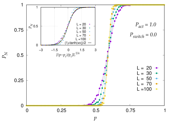
Figure 4: $P_{N}$ vs $p$ with $p_{act}=1.0$, $p_{switch}=0.00$ where $L=20,30,50,70$ and $100$ in the inset data collapse has been shown as $\frac{(1+\tanh(\kappa x))}{2}$ with $n=1.5$, and $\kappa=1.4$

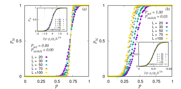
Figure 5: $P_{N}$ vs $p$ where $L=20,30,50,70$ and $100$ with $n=1.5$, $(a)$ $p_{act}=0.80$ and $p_{switch}=0.00$ in the inset data colaps has been shown as $\frac{(1+\tanh(\kappa x))}{2}$, $n=1.5$ and $\kappa=1.5$ $(b)$ $p_{act}=1.0$ and $p_{switch}=0.03$ in the inset data collapse has been shown as $\frac{(1+\tanh(\kappa(x-\epsilon))}{2}$, $n=3.5$, $\kappa=0.47$ and $\epsilon=6.31$.

It is interesting to study the delay of arrival of the signal at the receiving end by analyzing the paths of the Active cells for the cases when $p_{switch}=0.0$. For this we have calculated the Tortuosity $\tau$ [5], which is defined as,

$$\tau=\frac{\braket{l_{0}}}{L}=\frac{x_{0}}{L}$$ (5)

where $\braket{l_{0}}=x_{0}$ is the average path length.

Of course, $\tau$ depends on percolation probability $p$, since below critical percolation $p_{c}$ signal cannot be transmitted through the system. The variation of $x_{0}$ as a function of $p$ is shown in Fig. 6 and $\tau$ as a function of $p$ is shown in the inset of the same Figure in log scale for $L=20,30,50,70$ and $100$.It has been observed that

$$\tau\propto(p-p_{c})^{-u}$$ (6)

The exponent $u$ is almost independent of $L$ and the approximated value is $u\simeq 0.20$. It is to be mentioned here that value of this exponent remains unaltered with variation of $p_{act}$.

Figure 6: $x_{0}$ vs $p$ with $p_{act}=1.00$ and $p_{switch}=0.0$ and $L=20,30,50,70$ and $100$ n the inset data collapse has been shown as $\tau$ vs $p$ with $u\simeq 0.20$.

.3 Study of Cluster Distribution and Critical Exponents

Now we would move on to find out some other relevant exponents for the system. It is well known that the cluster distribution for site percolation shows power law behaviour for $p=p_{c}$ as $n(s)_{p_{c}}\propto s^{-{\Delta}}$ where $\Delta$ is the Fisher exponent [11].

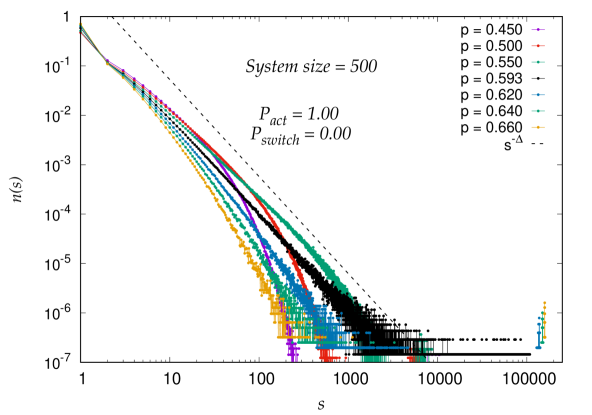
Figure 7: $n(s)$ vs $s$ with $L=500$, $p_{act}=1.00$ and $p_{switch}=0.0$ here $\Delta\simeq 1.96$.

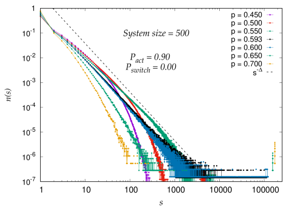
Figure 8: $n(s)$ vs $s$ with $L=500$, $p_{act}=0.90$ and $p_{switch}=0.0$ here $\Delta\simeq 1.91$.

The cluster distribution for $p_{act}=1.0$ and $p_{switch}=0.0$ for the cluster of Inactive sites is shown in Fig. 7. Here HK algorithm has been used to study [30] the cluster distribution. Here $\Delta$ is found to be close to $1.9$. The distribution is shown not only for $p_{c}$ but also above and below $p_{c}$. This nicely agrees with [31]. In Fig. 8 the cluster distribution is shown for $p_{act}=0.9$ and $p_{switch}=0.0$.

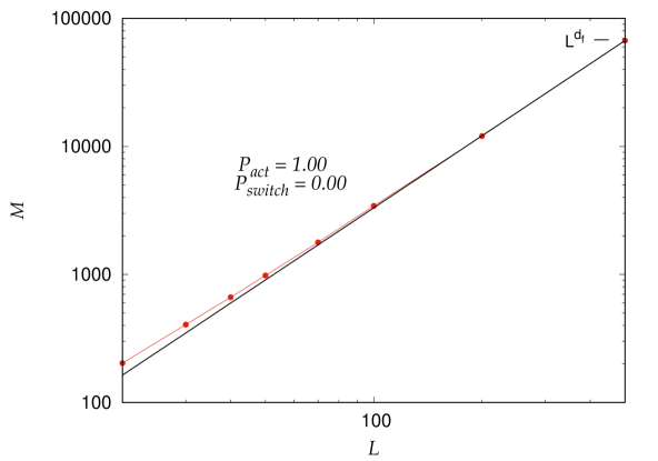
Figure 9: $M$ vs $L$ with $p_{act}=1.00$ and $p_{switch}=0.0$ here $d_{f}=1.81\pm 0.01$.

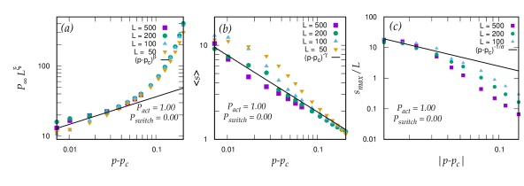
Figure 10: Study of critical exponents, (a) $P_{\infty}L^{\xi}$ vs $p-p_{c}$ with $\beta=0.39\pm 0.04$ and $\xi=1.95$, (b) $\braket{s}$ vs $p-p_{c}$ with $\gamma=0.60\pm 0.02$ and (c) $\frac{s_{max}}{L}$ vs $|p-p_{c}|$ with $\sigma=1.00\pm 0.33$, which clearly satisfy the relation $\beta+\gamma=\frac{1}{\sigma}$.

Mass of the largest cluster $M$ for $p=p_{c}$ shows a typical behaviours $M\sim L^{d_{f}}$ where $L$ is the system size and $d_{f}$ is the fractal dimension. This is shown in Fig. 9. Here $d_{f}$ is found to be $d_{f}=1.81\pm 0.01$.

From the values of system dimension $d$ and fractal dimension $d_{f}$ we may find $\Delta$ from the hyperscaling relation $\Delta=\frac{d}{d_{f}}+1$. The value of $\Delta$ thus obtained is close to $2.10$. However, as mentioned earlier, we have obtained a smaller value for $\Delta$.

The strength of the infinite cluster $P_{\infty}$ and the divergence of the mean cluster size $\langle s\rangle$ are another two important quantities. Those result in two more exponents $\beta$ and $\gamma$ which for our case happens to be $0.39\pm 0.04$ and $0.60\pm 0.02$ and are respectively shown in Fig. 10 (a) and (b).

From Fig. 7 another quantity is studied very often which is the cut-off cluster size $s_{max}$. This can be found from Fig. 7 (c) by using the well known form of $n_{s}\sim s^{-\Delta}\exp(-s/s_{max})$ for large $s$. The corresponding variation of cut-off cluster size $s_{max}$ for our system is shown in Fig. 10. From this we found the exponent $\sigma$ as $1.00\pm 0.33$, the relation being $s_{max}\propto(p-p_{c})^{-1/\sigma}$.

The value of the exponent $\alpha$ can be found out easily as $\sum_{0}^{\infty}n_{s}=(p-p_{c})^{2-\alpha}$. The value of $\alpha$ obtained in our case is close to $2.00$.

It is clear from the above facts that the Rushbrooke’s inequality $\alpha+2\beta+\gamma\geq 2$ is satisfied. Also the relation $\beta+\gamma=\frac{1}{\sigma}$ is verified here to be true.

Summary and Discussions

In summary, the work may be considered to have two aspects. Firstly, we tried to model the heart based on percolation theory and have studied several related features. Secondly, we have extracted the relevant exponents from the model so obtained.

In the first part, as mentioned, the signal propagation through the heart have been studied. It is known that the structure as well as the physiological processes in the heart are the key factors depending on which the signal propagates. We treat the heart as a 2D square grid of $L\times L$ cells which may be “Waiting (0)”, “Active(1)” and “Inactive(2)”. We started from some initial distribution of $0$s and $2$s. As the signal (AP) propagates, there are $1$s (Active sites) too. We considered two varieties: 1. When $2\rightarrow 0$ transition is allowed, i.e., $p_{switch}\neq 0$ and $p_{act}=1$; 2. When $2\rightarrow 0$ transition is not allowed, i.e., $p_{switch}=0$ and $p_{act}\neq 1$. We studied several important quantities. The number of arrival $N_{A}$ at the other side of the grid shows a Gaussian behaviour when $p_{act}$ is varying and $p_{switch}=0.0$. This indicates a kind of inhibitory behaviour and the AP/signal simply passes down the system within a fixed time. After that no new signal can pass down through the system as the cells are in their refractory period for an infinitely long time, indicating a damaged heart. However, the number of arrival $N_{A}$ at the other side of the grid shows a damped oscillatory behaviour when $p_{act}=1.0$ and $p_{switch}$ is varying, saturating to a finite value for high $p_{switch}$. This indicates that there are always a finite number of active cells and therefore new APs can pass through the system. It is to be noted that very high value of $p_{switch}$ has a disadvantage as the AP is trapped within the system which may be a cause for irregular heart rhythms.

In the other part of the work we have studied the percolation model of the system. It has been observed that the critical probability for percolation $p_{c}$ is close to $0.5923$ for the $p_{switch}=0$ and $p_{act}=1$. The value of $p_{c}$ shifts towards higher and higher side as $p_{act}$ is made smaller and smaller. Keeping $p_{act}$ fixed at $1$ and changing $p_{switch}$ a little has severe effect on $p_{c}$ and it shifts abruptly towards $0$. The tortuosity is studied and the related exponent is obtained as close to $0.2$. We also focused on the study of the exponents relevant to percolation theory. In this part we considered the parameters $p_{switch}=0$ and $p_{act}=1$ only. The cluster distribution is studied here as shown in Fig. 7. From this we checked the exponents $\alpha,\beta,\gamma,\sigma$ etc. The Rushbrooke Inequality $\alpha+2\beta+\gamma\geq 2$ and the relation $\beta+\gamma=1/\sigma$ has been observed to be satisfied.

Acknowledgement

AM acknowledges financial support from CSIR (SRF Grant no. 08/0463(12870)/2021-EMR-I). AM and SG acknowledges the computational facility of Vidyasagar College.

References

- [1] S. R. Broadbent and J. M. Hammersley, Percolation processes, Mathematical Proceedings of the Cambridge Philosophical Society. 53 (3) (1957) 629–641. https://doi.org/10.1017/S0305004100032680.
- [2] U. Dobramys, M. Mobilia, M. Pleimling and U. C. Täuber, Stochastic population dynamics in spatially extended predator–prey systems, J. Phys. A Math. Theor. 51 (2018) 063001. https://doi.org/10.1088/1751-8121/aa95c7.
- [3] H. Barghathi, T. Vojta and J. A. Hoyos, Contact process with temporal disorder, Phys. Rev. E 94 (2016) 022111. https://doi.org/10.1103/PhysRevE.94.022111.
- [4] E. Vigmond, A. Pashaei, S. Amraoui, H. Cochet and M. Hassaguerre, Percolation as a mechanism to explain atrial fractionated electrograms and reentry in a fibrosis model based on imaging data, Heart Rhythm 13 (2016) 1536. https://doi.org/10.1016/j.hrthm.2016.03.019.
- [5] S. A. Niederer, J. Lumens and N. A. Trayanova, Computational models in cardiology, Nat. Rev. Cardiol. 16 (2019) 100. https://doi.org/10.1038/s41569-018-0104-y.
- [6] R. Rabinovitch, Y. Biton, D. Braunstein, I.Aviram, R. Thieberger and A. Rabinovitch, Percolation and tortuosity in heart-like cells, Scientific Reports 11(1) (2021) 11441. https://doi.org/10.1038/s41598-021-90892-2.
- [7] S. Biswas, S. Roy and P. Ray, Nucleation versus percolation: Scaling criterion for failure in disordered solids, Phys. Rev. E 91 (2015) 050105(R). https://doi.org/10.1103/PhysRevE.91.050105.
- [8] A. K. Chandra Percolation in a kinetic opinion exchange model, Physical Review E 85 (2012) 021149. https://doi.org/10.1103/PhysRevE.85.021149.
- [9] F. Bagnoli, G. de B. Cavalcabo’, A Simple Model of Knowledge Percolation, archive, arXiv:2206.03267 (2022). https://doi.org/10.48550/arXiv.2206.03267.; B. Chopard, S. Bandini, A. Dennunzio, A. Haddad, Mira (eds) Cellular Automata. ACRI 2022. Lecture Notes in Computer Science, Springer, Cham. 13402 (2022). https://doi.org/10.1007/978-3-031-14926-9.
- [10] P. Bak, K. Chen and C. Tang, A forest-fire model and some thoughts on turbulence, Phys. Lett. A 147 (1990) 297. http://dx.doi.org/10.1016/0375-9601(90)90451-S.; P. Bak, C. Tang and K. Wiesenfeld, Self-organized criticality, Phys. Rev. A 38 (1988) 364. https://doi.org/10.1103/PhysRevA.38.364.
- [11] D. Stauffer and A. Aharony, Introduction to Percolation Theory, Taylor & Francis, (1994). https://doi.org/10.1201/9781315274386.
- [12] H. S. Song and S. H. Lee, Effects of wind and tree density on forest fire patterns in a mixed-tree species forest, Forest Science and Technology, 13(1) (2016) 9-16. http://dx.doi.org/10.1080/21580103.2016.1262793.
- [13] B. Drossel, and F. Schwabl, Self-organized critical forest-fire model, Phys. Rev. Lett. 69 (1992) 1629. https://doi.org/10.1103/PhysRevLett.69.1629.
- [14] W. K. Moner,B. Drossel, and F. Schwabl, Computer simulations of the forest-fire model, Phys. A Stat. Mech. Appl. 190(3) (1992) 205-217. https://doi.org/10.1016/0378-4371(92)90032-L.
- [15] D. Knežević, M. Knežević. Semi-directed percolation in two dimensions, Physica A 444 (2016) 560–565. https://doi.org/10.1016/j.physa.2015.10.079.
- [16] S. Redner, Conductivity of random resistor-diode networks, Phys. Rev. B 25 (1982) 5646–5655. https://doi.org/10.1103/PhysRevB.25.5646.
- [17] H. O. Mártin and J. Vannimenus, Partially directed site percolation on the square and triangular lattices, J. Phys. A: Math. Gen. 18 (1985) 1475-1482. 10.1088/0305-4470/18/9/027.
- [18] R. F. Gibson, A review of recent research on mechanics of multifunctional composite materials and structures, Composite Structures 92, (2010) 2793–2810. http://dx.doi.org/10.1016/j.compstruct.2010.05.003.
- [19] V. Langlois, V. H. Trinh, and C. Perrot, Electrical conductivity and tortuosity of solid foam: effect of pore connections, Phys. Rev. E 100 (2019) 013115. https://doi.org/10.1103/PhysRevE.100.013115.
- [20] B. Ghanbarian, A. G. Hunt, M. Sahimi, R. P. Ewing, and T. E. Skinner, Percolation theory generates a physically based description of tortuosity in saturated and unsaturated porous media, Soil Sci. Soc. Am. J. 77 (2013) 1920. http://dx.doi.org/10.2136/sssaj2013.01.0089.
- [21] D. S. Desai and S. Hajouli, Arrhythmias, StatPearls [Internet]. Treasure Island (FL): StatPearls Publishing, (2023) PMID: 32644349.
- [22] O. Dössel , M. W. Krueger, F. M. Weber, M. Wilhelm and G. Seemann, Computational modeling of the human atrial anatomy and electrophysiology, Med. Biol. Eng. Comput. 50 (2012) 773–799. https://doi.org/10.1007/s11517-012-0924-6.
- [23] A. Shirakabe, Y. Ikeda, S. Sciarretta, D. K. Zablocki, J. Sadoshima, Aging and Autophagy in the Heart. Circ Res. 118(10) (2016) 1563-1576, PMID: 27174950, PMCID: PMC4869999. https://doi.org/10.1161%2FCIRCRESAHA.116.307474.
- [24] P. Anversa, A. Leri, Innate regeneration in the aging heart: healing from within, Mayo Clin Proc. 88(8) (2013) 871-883, PMID: 23910414, PMCID: PMC3936323. https://doi.org/10.1016/j.mayocp.2013.04.001
- [25] D. L. Johnson, J. Koplik and R. Dashen, Theory of dynamic permeability and tortuosity in fluidsaturated porous media, Journal of Fluid Mechanics, 176 (1987) 379402. https://doi.org/10.1017/S0022112087000727.
- [26] B. Derrida and D. Stauffer, Corrections to scaling and phenomenological renormalization for 2-dimensional percolation and lattice animal problems, Journal de Physique 46 (1985) 1623. http://dx.doi.org/10.1051/jphys:0198500460100162300.
- [27] K. Malarz and S. Galam, Square-lattice site percolation at increasing ranges of neighbor bonds, Physical Review E 71 (2005) 016125. https://doi.org/10.1103/PhysRevE.71.016125.
- [28] X. Feng, Y. Deng, H. W. J. Blöte, Percolation transitions in two dimensions, Physical Review E 78 (2008) 031136. https://doi.org/10.1103/PhysRevE.78.031136.
- [29] S. Mertens, Exact site-percolation probability on the square lattice, J. Phys. A: Math. Theor. 55 (2022) 334002. https://doi.org/10.1088/1751-8121/ac4195.
- [30] J. Hoshen and R. Kopelman, Percolation and cluster distribution. I. Cluster multiple labeling technique and critical concentration algorithm, Phys. Rev. B 14 (1975) 3438. https://doi.org/10.1103/PhysRevB.14.3438.
- [31] M. Nicodemi, Percolation, Complexity Science & Theor. Phys., University of Warwick. lesson percolation.pdf