Reconstructing a pseudotree from the distance matrix of its boundary

Abstract

A vertex $v$ of a connected graph $G$ is said to be a boundary vertex of $G$ if for some other vertex $u$ of $G$, no neighbor of $v$ is further away from $u$ than $v$. The boundary $\partial(G)$ of $G$ is the set of all of its boundary vertices.

The distance matrix $\hat{D}_{G}$ of the boundary of a graph $G$ is the square matrix of order $\kappa$, being $\kappa$ the order of $\partial(G)$, such that for every $i,j\in\partial(G)$, $[\hat{D}_{G}]_{ij}=d_{G}(i,j)$.

Given a square matrix $\hat{B}$ of order $\kappa$, we prove under which conditions $\hat{B}$ is the distance matrix $\hat{D}_{T}$ of the set of leaves of a tree $T$, which is precisely its boundary.

We show that if $G$ is either a tree or a unicyclic graph with girth $g\geq 5$ vertices, then $G$ is uniquely determined by the distance matrix $\hat{D}_{G}$ of the boundary of $G$ and we also conjecture that this statement holds for every connected graph.

Moreover, two algorithms for reconstructing a tree and a unicyclic graph from the distance matrix of their boundaries are given, whose time complexities in the worst case are, respectively, $O(\kappa n)$ and $O(n^{2})$.

1 Introduction

While typically a graph is defined by its lists of vertices and edges, significant research has been dedicated to minimizing the necessary information required to unequivocally determine a graph. For example, various approaches include reconstructing metric graphs from density functions [9], road networks from a set of trajectories [1], graphs utilizing shortest path or distance oracles [15], labeled graphs from all r-neighborhoods [19], or reconstructing phylogenetic tree [2]. Of particular note is the graph reconstruction conjecture [16, 26] which states the possibility of reconstructing any graph on at least three vertices (up to isomorphism) from the multiset of all unlabeled subgraphs obtained through the removal of a single vertex. Indeed, a search with the words “graph reconstruction” returns more than 3 million entries.

In this paper, our focus lies in the reconstruction of graphs from the distance matrix of their boundary vertices and the graph’s order. We are persuaded that this process could hold true for all graphs and we state it as a conjecture (see Conjecture 35). However, it is of particular interest to explore whether this conjecture holds for specific families of graphs. Our objective herein is to establish its validity for pseudotrees, i.e., for both trees and unicyclic graphs.

The concept of a graph’s boundary was introduced by Chartrand, Erwin, Johns and Zhang in 2003 [7]. Initially conceived to identify local maxima of vertex distances, the boundary has since revealed a host of intriguing properties. It has been recognized as geodetic [4], serving as a resolving set [13], and also as a strong resolving set [21]. Put simply, each vertex lies in the shortest path between two boundary vertices and, given any pair of vertices $x$ and $y$, there exists a boundary vertex $v$ such that either $x$ lies on the shortest path between $v$ and $y$, or vice versa. With such properties, it is unsurprising that the boundary emerges as a promising candidate for reconstructing the entire graph.

Graph distance matrices represent a fundamental tool for graph users, enabling the solution of problems such as finding the shortest path between two nodes. However, our focus here shifts mainly towards their realizability. That is, given a matrix (symmetric, with positive integer entries, and zeroes on the diagonal), we inquire whether there exists a corresponding graph where the matrix entries represent the distances between vertices. In 1965, Hakimi and Yau [11] established Theorem 7 presenting a straightforward additional condition that the matrix must satisfy to be realizable. Building upon this, in 1974, Peter Buneman [3] provided the matrix characterization for being the distance matrix of a tree once we know that the graph is $K_{3}$-free, and Graham and Pollack [10] computed the determinant of the distance matrix of a tree (see Theorem 16). Additionally, Edward Howorka [14] in 1979, formulate conditions for a distance matrix of a block graph (see Theorem 14), and Lin, Liu and Lu [18] provided the determinant of such matrices (see Theorem 15). Incidentally, we use their result to derive the converse of the Graham and Pollack’s theorem. Furthermore, we also give an algorithmic approach to the characterization of the distance matrix of a unicyclic graph.

As previously mentioned, our focus lies on the distance matrix of a graph’s boundary, a subset of the overall distance matrix. We seek to determine the realizability of these matrices and, while we have achieved characterization in the case of trees, a similar analysis for unicyclic graphs remains elusive.

Finally, we present various algorithms for reconstructing trees and unicyclic graphs from the distance matrix of their boundary. In trees, the boundary corresponds to the leaves, while in unicyclic graphs, it contains the leaves along with the vertices of the cycle with degree two. Notably, the concept of doubly resolving sets, introduced in [5], proves instrumental in these reconstructions.

The paper is organized as follows: this section is finished by introducing general terminology and notation. In Section 2, we explore the notion of boundary and its relation with distance matrices. Section 3 is devoted to the reconstruction of trees, completing first with the realizability of distance matrices of a tree, and of the boundary of a tree. Following this, Section 4 undertakes the characterization of distance matrices for unicyclic graphs, followed by their reconstruction from boundary distance matrices. Finally, the paper ends with a section on conclusions and open problems.

1.1 Basic terminology

Let us introduce some basic notation that is going to be useful thorough the paper. All the graphs considered here are undirected, simple, finite and (unless otherwise stated) connected. If $G=(V,E)$ is a graph of order $n$ and size $m$, it means that $|V|=n$ and $|E|=m$. Unless otherwise specified, $n\geq 2$ and $V=[n]=\{1,\ldots,n\}$.

Let $v$ be a vertex of a graph $G$. The open neighborhood of $v$ is $N(v)=\{w\in V(G):vw\in E\}$, and the closed neighborhood of $v$ is $N[v]=N(v)\cup\{v\}$ . The degree of $v$ is $\deg(v)=|N(v)|$. The minimum degree (resp. maximum degree) of $G$ is $\delta(G)=\min\{\deg(u):u\in V(G)\}$ (resp. $\Delta(G)=\max\{\deg(u):u\in V(G)\}$). If $\deg(v)=1$, then $v$ is said to be a leaf of $G$ and the set and the number of leaves of $G$ are denoted by ${\cal L}(G)$ and $\ell(G)$, respectively.

Let $K_{n}$, $P_{n}$, $W_{n}$ and $C_{n}$ be, respectively, the complete graph, path, wheel and cycle of order $n$. Moreover, $K_{r,s}$ denotes the complete bipartite graph whose maximal independent sets are $\overline{K_{r}}$ and $\overline{K_{s}}$, respectively. In particular, $K_{1,n-1}$ denotes the star with $n-1$ leaves.

Let $W\subseteq V(G)$. The subgraph of $G$ induced by $W$, denoted by $G[W]$, has $W$ as vertex set and $E(G[W])=\{vw\in E(G):v,w\in W\}$. If $G[W]$ is a complete graph, then it is said to be a clique of $G$.

Given a pair of vertices $u,v$ of a graph $G$, a $u-v$ geodesic is a $u-v$ shortest path, i.e., a path joining $u$ and $v$ of minimum order. Clearly, the length of all $u-v$ geodesics are the same, and it is called the distance between vertices $u$ and $v$ in $G$, denoted by $d_{G}(u,v)$, or simply by $d(u,v)$, when the context is clear. A set $W\subseteq V(G)$ is called geodetic if any vertex of the graph is in a $u-v$ geodesic with $u,v\in W$. In particular, three vertices in a cycle $C$ are called a geodetic triple if they are geodetic for $V(C)$.

The eccentricity $\rm ecc(v)$ of a vertex $v$ is the distance to a farthest vertex from $v$. The radius and diameter of $G$ are respectively, the minimum and maximum eccentricity of its vertices and are denoted as ${\rm rad}(G)$ and ${\rm diam}(G)$. A vertex $u\in V(G)$ is a central vertex $G$ if $\rm ecc(u)={\rm rad}(G)$, and it called a peripheral vertex of $G$ if $\rm ecc(u)={\rm diam}(G)$. The set of central (resp., peripheral) vertices of $G$ is called the center (resp., periphery) of $G$.

Let $S=\{w_{1},w_{2},\ldots,w_{k}\}$ be a set of vertices of a graph $G$. The distance between a vertex $v\in V(G)$ and $S$, denoted by $d(v,S)$, is the minimum of the distances between $v$ and the vertices of $S$, that is, $d(v,S)=\min\{d(v,w):w\in S\}$. The metric representation $r(v|S)$ of a vertex $v$ with respect to $S$ is defined as the $k$-vector $r(v|S)=(d_{G}(v,w_{1}),d_{G}(v,w_{2})\ldots,d_{G}(v,w_{k}))$. A set of vertices $S$ of $G$ is called resolving if for every pair of distinct vertices $x,y\in V(G)$, then $r(x|S)\neq r(y|S)$.

Resolving sets were first introduced by Slater in [24], and since then, many other similar concepts have been defined, particularly, we deal with doubly resolving [5] and strong resolving sets [22, 20] in this paper. Thus, the set $S$ is doubly resolving if for every $x,y\in V(G)$, there exists $u,v\in S$ such that $d(x,u)-d(y,u)\neq d(x,v)-d(y,v)$. Another way to see it is that $r(x|S)-r(y|S)\neq(a,\stackrel{{\scriptstyle|S|}}{{\ldots}},a)$ for any integer $a$. On the other hand, $S$ is a strong resolving if for every pair of distinct vertices $x,y\in V(G)$ either $x$ is in a $v-y$ geodesic or $y$ is in $u-x$ geodesic where $v\in S$. In other words, $S$ is a strong resolving set if, for every distinct vertices $x,y\in V(G)$ , there is a vertex $v\in S$, such that either $d(x,v)=d(x,y)+d(y,v)$ or $d(y,v)=d(y,x)+d(x,v)$. Clearly, every strong or doubly resolving sets are also resolving, being the converse far from true (see Figure 1).

A graph $G$ with the same order as size is called unicyclic. These graphs contain a unique cycle that is denoted as $C_{g}$ where $g$ is the girth. The connected component of $G-E(C_{g})$ containing a vertex $v\in V(C_{g})$ is denoted as $T_{v}$ and it is called the branching tree of $v$. The tree $T_{v}$ is said to be trivial if $V(T_{v})=\{v\}$. A vertex $v\in V(G)$ is a branching vertex if either $v\not\in V(C_{g})$ and $\deg(v)\geq 3$ or $v\in V(C_{g})$ and $\deg(v)\geq 4$.

A connected graph $G$ of order $n$ and size $m$ is called a pseudotree if $m-1\leq n\leq m$, i.e., if it is either a tree (including a path) or a unicyclic graph (including a cycle).

A cut-vertex is a vertex whose deletion disconnects the graph. If $G$ has no cut-vertices, then it is called a block. A maximal subgraph of $G$ without cut-vertices is a block of $G$. In a block graph, every block is a clique, or equivalently, if every cycle induces a complete subgraph.

For additional details and information on basic Graph Theory we refer the reader to [8].

2 The conjecture

2.1 Boundary of a graph

In this subsection, we introduce one of the essential components of our work: the boundary of a graph which was first studied by Chartrand et al. in [7]. A vertex $v$ of a graph $G$ is said to be a boundary vertex of a vertex $u$ if no neighbor of $v$ is further away from $u$ than $v$, i.e., if for every vertex $w\in N(v)$, $d(u,w)\leq d(u,v)$. The set of boundary vertices of a vertex $u$ is denoted by $\partial(u)$. Given a pair of vertices $u,v\in V(G)$ if $v\in\partial(u)$, then $v$ is also said to be maximally distant from $u$. A pair of vertices $u,v\in V(G)$ are said to be mutually maximally distant, or simply $MMD$, if both $v\in\partial(u)$ and $u\in\partial(v)$.

The boundary of $G$, denoted by $\partial(G)$, is the set of all of its boundary vertices, i.e., $\partial(G)=\cup_{u\in V(G)}\partial(u)$. Notice that, as was pointed out in [21], the boundary of $G$ can also be defined as the set of $MMD$ vertices of $G$, i.e.,

$$\partial(G)=\{v\in V(G):{\rm there\,exists}\,u\in V(G)\,{\rm such\,that}\,u,v\,{\,\rm are}\,MMD\}$$

Thorough the paper, the cardinality of the boundary is denoted by $\kappa$. The graphs with small $\kappa$ have been completely characterized by the following theorem.

Theorem 1 ([12, 25]).

Let $G$ be a graph of order $n\geq 2$. Then, $\kappa=2$ if and only if $G=P_{n}$. Moreover, $\kappa=3$ if and only if either

1. $G$ is a subdivision of $K_{1,3}$; or

2. $G$ can be obtained from $K_{3}$ by attaching exactly one path (of arbitrary length) to each of its vertices.

Also, graphs with a big $\kappa$ are well-known, as the next results show.

Proposition 2.

Given a graph $G$ be a graph of order $n$.

1. If ${\rm rad}(G)={\rm diam}(G)$, then $\kappa=n$.

2. If ${\rm diam}(G)=2$, then $n-1\leq\kappa\leq n$.
   Moreover, $\kappa=n-1$ if and only if contains a unique central vertex.

Proof.

1. Suppose that ${\rm rad}(G)={\rm diam}(G)=d$. Take $u\in V(G)$ and notice that $\rm ecc(u)=d$. Let $v\in V(G)$ such that $d(u,v)=d$. For every vertex $w\in N(v)$, $d(u,w)\leq d=d(u,v)$. Hence, $u\in\partial(u)\subseteq\partial(G)$.

2. If ${\rm rad}(G)={\rm diam}(G)=2$, then according to the previous item, $\kappa=n$. Suppose that ${\rm rad}(G)=1$. Let $V(G)=U\cup W$ such that $U$ is the set of central vertices and $W$ is the set of peripheral vertices of $G$. Observe that $W\subsetneq\partial(G)$ and that if $|U|=h$, then $G[U)]=K_{h}$. If $h\geq 2$, then every central vertex belongs to the boundary of every other vertex of $G$. If $h=1$ and $U=\{u\}$, then for every vertex $w\in W$, $u\not\in\partial(w)$, i.e., $\partial(G)=W$, which means that $\kappa=|W|=n-1$.

∎

Corollary 3.

Let $G$ be a graph of order $n\geq 3$.

1. If $G\in\{K_{n},K_{r,s},C_{n}\}$ and $r,s\geq 2$, then $\kappa=n$.

2. If $G\in\{W_{n},K_{1,n-1}\}$, then $\kappa=n-1$.

As previously mentioned, the boundary exhibits several intriguing properties, like being geodetic [4] and a resolving set [13]. However, for the scope of this paper, its status as a strong resolving set is particularly pertinent. Thus, we shall now develop into this concept with some detail.

That notion were first defined by Sebő and Tannier [22] in 2003, and later studied in [20]. They were interested in extending isometric embeddings of subgraphs into the whole graph and, to ensure that, defined a strong resolving set of a graph $G$ as a subset $S\subseteq V(G)$ such that for any pair $x,y\in V(G)$ there is an element $v\in S$ such that there exists a $x-v$ geodesic that contains $y$, or a $y-v$ geodesic containing $x$. What is crucial for our goals is that, as a consequence of the definition, it only suffices to know the distances from vertices of a strong resolving set to the rest of the nodes, to determine the graph unequivocally. This is explored in more detail in Subsection 2.2.

It turns out that the boundary is always a strong resolving set.

Proposition 4 ([21]).

The boundary $\partial(G)$ of every graph $G$ is a strong resolving set.

Proof.

Let $u,v\in V(G)$ such that $d(u,v)=k$ and $\{u,v\}\cap\partial(G)=\emptyset$. So, for some vertex $w_{1}\in N(v)$, $d(u,w_{1})=k+1$. If $w_{1}\in\partial(u)$, then we are done. Otherwise, for some vertex $w_{2}\in N(w_{1})$, $d(u,w_{2})=k+2$. Thus, after iterating this procedure finitely many times, say $h$ times, we will find a vertex $w_{h}$ such that for every vertex $w\in N(w_{h})$, $d(u,w)\leq d(u,w_{h})=k+h$, i.e., a vertex $w_{h}\in\partial(G)$ and a $u-w_{h}$ geodesic containing vertex $v$. ∎

Particularly, for trees and unicyclic graphs, the boundary is very straightforward to characterize. Nevertheless, those results will be extensively used thorough this work.

Proposition 5 ([25]).

Let $T$ be a tree. Then, $\partial(T)={\cal L}(T)$.

Proof.

If $u\in{\cal L}(T)$ and $N(u)=\{v\}$, then notice that $u\in\partial(v)$.

Take $u\in V(T)$ such that $\deg(u)\geq 2$. If $\{v_{1},v_{2}\}\subseteq N(u)$, then, for every vertex $w\in V(T)$, $d(w,u)<\max\{d(w,v_{1}),d(w,v_{2})\}$. Hence, $u\not\in\partial(G)$. ∎

Proposition 6.

Let $G=(V,E)$ be a unicyclic graph. If ${\cal U}(G)$ denotes the set of vertices of $C_{g}$ of degree 2, then $\partial(G)={\cal L}(G)\cup{\cal U}(G)$.

Proof.

If $u\in{\cal L}(G)$ and $N(u)=\{v\}$, then notice that $u\in\partial(v)$.

Let $u\in{\cal U}(G)$. Let $v\in V(C_{g})$ such that $d(u,v)\in\lfloor\frac{g}{2}\rfloor$. If $w$ is a leaf of the branching tree $T_{v}$ of $v$, then observe that $u\in\partial(w)$.

Finally, take a vertex $u\not\in{\cal L}(G)\cup{\cal U}(G)$. If $u\in V(C_{g})$, $N(u)\cap V(C_{g})=\{v_{1},v_{2}\}$ and $v_{3}\in N(u)\cap V(T_{u})$, then $d(w,u)<\max\{d(w,v_{1}),d(w,v_{2}),d(w,v_{3})\}$, for every vertex $w\in V(G)$. Hence, $u\not\in\partial(G)$. If $u\in V(T_{v})$ for some vertex $v\in V(C_{g})$, $\deg(u)\geq 2$ and $\{v_{1},v_{2}\}\subseteq N(u)$, then $d(w,u)<\max\{d(w,u_{1}),d(w,v_{2})\}$, for every vertex $w\in V(G)$. Hence, $u\not\in\partial(G)$. ∎

2.2 Distance matrix of a graph

At this point, the other relevant element of the work is introduced: distance matrices. Some notation is provided as well as a complete characterization of the distance matrix of a tree and the distance matrix of the leaves of a tree. The subsection is finished with our main conjecture and the development of the ideas that justify it.

A square matrix $D$ is called a dissimilarity matrix if it is symmetric, all off-diagonal entries are (strictly) positive and the diagonal entries are zeroes. A square matrix $D$ of order $n$ is called a metric dissimilarity matrix if it satisfies, for any triplet $i,j,k\in[n]$, the triangle inequality: $d_{ik}\leq d_{ij}+d_{jk}$.

The distance matrix $D_{G}$ of a graph $G=(V,E)$ with $n$ vertices is the square matrix of order $n$ such that, for every $i,j\in[n]$, $d_{ij}=d(i,j)$. Certainly, this matrix is a metric dissimilarity matrix. A metric dissimilarity matrix $D$ is called a distance matrix if there is graph $G$ such that $D_{G}=D$.

Let $S$ be a subset of vertices of order $k$ of a graph $G=([n],E)$. It is denoted by $D_{S,V}$ the submatrix of $D_{G}$ of order $k\times n$ such that for every $i\in S$ and for every $j\in V$, $[D_{S,V}]_{ij}=d(i,j)$. Similarly, the so-called $S$-distance matrix of $G$, denoted by $D_{S}$, is the square submatrix of $D_{G}$ of order $k$ such that for every $i,j\in S$, $[D_{S}]_{ij}=d(i,j)$. If $S=\partial(G)$, then $D_{S}$ is also denoted by $\hat{D}_{G}$ and called the distance matrix of the boundary of $G$.

The next result was stated and proved in [11] and constitutes a general characterization of distance matrices. We include here a (new) proof, for the sake of completeness.

Theorem 7 ([11]).

Let $D$ be an integer metric dissimilarity matrix of order $n$. Then, $D$ is a distance matrix if and only if, for every $i,j\in[n]$, if $d_{ij}>1$, then there exists an integer $k\in[n]$ such that

$d_{ik}=1$ and $d_{ij}=d_{ik}+d_{kj}$.

Proof.

The necessity of the above condition immediately follows from the definition of distance matrix.

To prove the sufficiency, we consider the non-negative symmetric square matrix $A$ of order $n$, such that, for every pair $i,j\in[n]$, $a_{ii}\in\{0,1\}$ being $a_{ij}=1$ if and only if $d_{ij}=1$. Let $G$ the graph $G=([n],E)$ of order $n$ such that its adjacency matrix is $A$. Next, we show that the distance matrix of $G$ is precisely $D$.

If ${\rm diam}(G)=d$, then $d(i,j)=p\in\{1,\ldots,d\}$, for every pair of distinct vertices $i,j\in[n]$. If $p=1$, then clearly $d(i,j)=1$ if and only if $d_{ij}=1$. Take $2\leq p\leq d$ and suppose that, if $1\leq r\leq p-1$, then

$$d(i,j)=r\,\,{\rm if\,\,and\,\,only\,\,if}\,\,d_{ij}=r$$

Let $i,j\in[n]$ such that $d_{ij}=p$. According to item (c), take $k\in[n]$ such that $d(i,k)=d_{ik}=1$ and $p=d_{ij}=d_{ik}+d_{kj}=1+d_{kj}$. This means that $d(i,j)\leq p$, since $d_{kj}=p-1$ and $d(i,j)\leq d(i,k)+d(k,j)=1+d(k,j)$. Hence, $d(i,j)=p$ as otherwise, according to the inductive hypothesis (1), $d_{ij}=d(i,j)<p$, a contradiction.

Conversely, let $i,j\in[n]$ such that $d(i,j)=p$. Let $k\in N(i)$ such that $d(i,j)=1+d(k,j)$. According to item (b), $d_{ij}\leq d_{ik}+d_{kj}$. This means that $d_{ij}\leq p$, since $d(k,j)=p-1$ and $d_{ij}\leq 1+d_{kj}$. Hence, $d_{ij}=p$ as otherwise, according to the inductive hypothesis (1), $d(i,j)=d_{ij}<p$, again a contradiction. ∎

An integer metric dissimilarity matrix $D$ of order $n$ is called additive if every subset of indices $\{i,j,h,k\}\subseteq[n]$ satisfies the so-named four-point condition:

$$\left\{\begin{array}[]{c}d_{ij}+d_{hk}\leq\max\{d_{ih}+d_{jk},d_{ik}+d_{jh}\}\\ \\ d_{ih}+d_{jk}\leq\max\{d_{ij}+d_{hk},d_{ik}+d_{jh}\}\\ \\ d_{ik}+d_{jh}\leq\max\{d_{ij}+d_{hk},d_{ih}+d_{jk}\}\\ \end{array}\right.$$

A graph $G=([n],E)$ is said to satisfy the four-point condition if its distance matrix $D_{G}$ is additive, that is, if every 4-vertex set $\{i,j,h,k\}\subseteq[n]=V(G)$ satisfies this condition, a strengthened version of the triangle inequality (see [3]):

$$\left\{\begin{array}[]{c}d(i,j)+d(h,k)\leq\max\{d(i,h)+d(j,k),d(i,k)+d(j,h)\}\\ \\ d(i,h)+d(j,k)\leq\max\{d(i,j)+d(h,k),d(i,k)+d(j,h)\}\\ \\ d(i,k)+d(j,h)\leq\max\{d(i,j)+d(h,k),d(i,h)+d(j,k)\}\\ \end{array}\right.$$

As was pointed out in [3], these inequalities can be characterized as follows.

Proposition 8 ([3]).

Let $\{i,j,h,k\}$ be a 4-vertex set of a graph $G=([n],E)$. Then, the following statements are equivalent.

1. $\{i,j,h,k\}$ satisfies the four-point condition.

2. Among the three sums $d(i,j)+d(h,k)$, $d(i,h)+d(j,k)$, $d(i,k)+d(j,h)$, the two largest ones are equal.

The next result was implicitly mentioned in some papers [17, 21, 22] and proved in [6]. This equivalence, along with statement shown in Proposition 4, has served as an inspiration for the main conjecture of the paper that is presented at the end of this subsection.

Theorem 9 ([6]).

Let $S$ be a proper subset of vertices of a graph $G=(V,E)$. Then, the following statements are equivalent.

1. $S$ is a strong resolving set.

2. $G$ is uniquely determined by the distance matrix $D_{S,V}$.

As was noticed in [21, 22], this result is not true if we consider resolving sets instead of strong resolving sets. For example, the pair of leaves of the graphs displayed in Figure 1 form a resolving set $S$ in both cases, and also for both graphs the matrix $D_{S,V}$ is the same.

Figure 1: A pair of graphs of order $7$, whose pair of leaves form a minimum (not strong) resolving set

As a direct consequence of both Theorem 9 and Proposition 4, the following result holds.

Corollary 10 ([12]).

Let $G=(V,E)$ be a graph. Then, $G$ is uniquely determined by the distance matrix $D_{\partial(G),V}$.

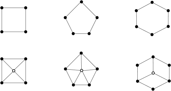
Figure 2: Three pairs of graphs having the same $\partial(G)$-distance matrix but different order. In all cases, the boundary $\partial(G)$ is the set of black vertices

On the other hand, it is relatively easy two find pairs of graphs having the same boundary (and thus also the same distance matrix of the boundary) but different order. See Figure 2, for three examples. Based on all of these results and particularly on the one stated in Corollary 10, we present the following conjecture.

Conjecture 11.

Let $\hat{B}$ a metric dissimilarity matrix of order $\kappa$. Let $G=([n],E)$ be a graph such that $\hat{D}_{G}=\hat{B}$. If $G^{\prime}=([n],E^{\prime})$ is a graph such that $\hat{D}_{G}=\hat{B}$, then $G$ and $G^{\prime}$ are isomorphic.

In other words, we are persuaded that, at least for many graph families, it is possible to obtain the whole graph $G$ from the $\partial(G)$-distance matrix. In Sections 3 and 4, we will prove this conjecture both for trees and unicyclic graphs.

3 Realizability and reconstruction of trees

This section is divided into three subsections: in the first one, we revise the main results regarding the characterization of tree distance matrices and we give the converse of the result of Graham and Pollack [10] in Theorem 18. The next subsection is devoted to determine those matrices which can be the ${\cal L}(T)$-distance matrix of a tree $T$, which is given in Theorem 23. Finally, in the last subsection, we describe and check the validity of the procedure to reconstruct a tree having its ${\cal L}(T)$-distance matrix as the only information. That completes our study on trees.

3.1 Distance matrices of a tree

In the seminal paper [3], Peter Buneman noticed that trees satisfy the four-point condition and also showed that a $K_{3}$-free graph is a tree if and only its distance matrix is additive. In the same paper, it was also proved that, for every additive matrix $A$ of order $k$, there always exists a weighted tree of order $n\geq k$ containing a subset of vertices $S$ of order $k$ such that $D_{S}=A$ (see Figure 3). A different approach based on the structure of the $4\times 4$ principal submatrices was given by Simões Pereira in [23]. In addition, it was proved in [27] that for every dissimilarity matrix $D$, it satisfies de four-point condition if and only if there is a unique weighted binary tree $T$ whose $\partial(T)$-distance matrix is $D$.

Starting from these results, Edward Howorka in [14] was able to characterize the family of graphs whose distance matrix is additive, i.e., satisfying the four-point condition. We include next new proofs of those results for the sake of both completeness and clarity.

Figure 3: A pair of graphs $G_{1}$ and $G_{2}$ of order 4 and 5 respectively, being $G_{2}$ a weighted tree, such that $D_{G_{1}}$, the distance matrix of $G_{1}$, and $D_{[4]}$, the $[4]$-distance matrix of $G_{2}$, are the same

Proposition 12 ([14]).

Every block graph satisfies the four-point condition.

Proof.

Let $S$ be a 4-vertex set of a block graph $G$, named $S=\{1,2,3,4\}$. The only seven possible configurations of paths connecting the 4 vertices of $S$ are those shown in Figure 4. We check that the four-condition holds in all cases.

1. $d_{12}+d_{34}=d_{13}+d_{24}=d_{14}+d_{23}=a+b+c+d$

2. $d_{12}+d_{34}=a+b+c+d$

   $d_{13}+d_{24}=d_{14}+d_{23}=a+b+c+d+2e$

3. $d_{12}+d_{34}=a+b+c+d$

   $d_{13}+d_{24}=d_{14}+d_{23}=a+b+c+d+2$

4. $d_{12}+d_{34}=a+b+c+d+1$

   $d_{13}+d_{24}=d_{14}+d_{23}=a+b+c+d+2e+2$

5. $d_{12}+d_{34}=a+b+c+d$

   $d_{13}+d_{24}=d_{14}+d_{23}=a+b+c+d+2$

6. $d_{12}+d_{34}=a+b+c+d+2$

   $d_{13}+d_{24}=d_{14}+d_{23}=a+b+c+d+2e+4$

7. $d_{12}+d_{34}=d_{13}+d_{24}=d_{14}+d_{23}=a+b+c+d+2$

∎

Figure 4: There are seven possible configurations of paths connecting 4 vertices of a block graph

The converse is proved in the next proposition.

Proposition 13 ([14]).

If $G$ satisfies the four-point condition, then it is a block graph.

Proof.

Let $C_{h}$ be an induced cycle of $G$ of minimum order $h\geq 4$. Then, $h=4q+r$, with $q\geq 1$ and $0\leq r\leq 3$. Notice that $C_{h}$ is not only an induced subgraph of $G$ but also isometric. Take a 4-vertex set $\{i,j,h,k\}\subseteq V(C_{h})$ such that $\{d_{ij},d_{jh},d_{h,k},d_{k,i}\}\subseteq\{q,q+1\}$. Check that $d_{ij}+d_{hk}\leq 2q+2$, $d_{ik}+d_{jh}\leq 2q+2$ and $d_{ih}+d_{jk}\geq 4q$. Hence, this 4-vertex set violate the four-point condition, which means that either $G$ is a tree or it is a chordal graph of girth 3, i.e., the only induced cycles have length 3.

Next, suppose that $G$ is a chordal graph of girth 3. Take a cycle $C_{p}=([p],E)$ in $G$ of minimum order $p\geq 4$, such that $[p]$ is not a clique. Notice that $p\geq 5$, since neither the cycle $C_{4}$ nor the diamond $K_{4}-e$ satisfies the four-point condition. Let $i,j\in[p]$ such that $1\leq i<j\leq p$ and $ij\not\in E(G)$. Notice that $d(i,j)=2$, since $C_{p}$ is of minimum order. W.l.o.g. we may assume that $i=1$ and $j=3$. Observe that for every $h\not\in\{2,p\}$ and $k\not\in\{2,4\}$, $\{1h,3k\}\cap E(G)=\emptyset$, since $C_{p}$ is of minimum order.

Let $h$ be the minimum integer between $4$ and $p$ such that $2h\in E(G)$. Then, clearly $h=4$, since otherwise the set $\{2,\ldots,h\}$ is an induced cycle of order at least 4, a contradiction. Let $k$ be the minimum integer between $5$ and $p$ such that $2k\in E(G)$. We distinguish cases.

Case 1. If $k=5$, then the subgraph induced by the set $\{2,3,4,5\}$ is the diamond $K_{4}-e$, a contradiction.

Case 2. If $p=5$ and $2k\in E(G)$, then the subgraph induced by the set $\{2,4,5,1\}$ is the cycle $C_{4}$, a contradiction.

Case 3. If $p\geq 6$ and $k\geq 6$, then the subgraph induced by the set $\{2,4,5,\ldots,k\}$ is the cycle $C_{k-2}$, a contradiction.

Hence, we have proved that every cycle of $G$ induces a clique, i.e., $G$ is a block graph. ∎

Once the two implications have been proved, we can establish the theorem.

Theorem 14 ([14]).

A graph $G$ of order $n$ is a block graph if and only if its distance matrix $D_{G}$ is additive.

Theorem 15 ([18]).

Let $G$ be a block graph on $n$ vertices and $k$ blocks $K_{n_{1}},\ldots,K_{n_{k}}$. Then,

$$\det({D_{G}})=(-1)^{n-1}\sum_{i=1}^{k}\frac{n_{i}-1}{n_{i}}\prod_{j=1}^{k}n_{j}$$

In particular, as a straight consequence of the previous result, the following theorem, proved in [10] is obtained.

Theorem 16 ([10]).

If $T$ is a tree on $n$ vertices, then $\det({D_{T}})=(-1)^{n-1}(n-1)2^{n-2}$.

The next lemma is the crucial result that allows to prove the characterization of distance matrices of trees by means of its determinant.

Lemma 17.

Let $k$ and $n$ integers such that $n\geq 3$ and $1\leq k\leq n-1$. Let $\{n_{1},\ldots,n_{k}\}$ a decreasing sequence of $k$ integers such that $n-1\geq n_{1}\geq\ldots\geq n_{k}\geq 2$ and $n_{1}+\ldots+n_{k}=n+k-1$. Then,

$$\sum_{i=1}^{k}\frac{n_{i}-1}{n_{i}}\prod_{j=1}^{k}n_{j}\leq(n-1)2^{n-2}$$

Moreover, the equality holds if and only if $k=n-1$ and $n_{1}=\ldots=n_{n-1}=2$.

Proof.

Let $h\in[k]$ such that $n_{h}\geq 3$ and for every $i\in\{h+1,\ldots,k\}$, $n_{i}=2$. Then,

$$\sum_{i=1}^{k}\frac{n_{i}-1}{n_{i}}\prod_{j=1}^{k}n_{j}=\Big{(}\frac{n_{1}-1}{n_{1}}+\ldots+\frac{n_{h}-1}{n_{h}}+\frac{k-h}{2}\Big{)}\cdot\prod_{j=1}^{h}n_{j}\cdot 2^{k-h}$$

Take the $(k+1)$-sequence $\{n^{\prime}_{1},\ldots,n^{\prime}_{k+1}\}=\{n_{1},\ldots,n_{h-1},n_{h}-1,n_{h+1},\ldots,n_{k},2\}$. Then,

$$\sum_{i=1}^{k+1}\frac{n^{\prime}_{i}-1}{n^{\prime}_{i}}\prod_{j=1}^{k+1}n^{\prime}_{j}=\Big{(}\frac{n_{1}-1}{n_{1}}+\ldots+\frac{n_{h-1}-1}{n_{h-1}}+\frac{n_{h}-2}{n_{h}-1}+\frac{k-h}{2}+\frac{1}{2}\Big{)}\cdot\prod_{j=1}^{h-1}n_{j}\cdot\frac{n_{h}-2}{n_{h}-1}\cdot 2^{k-h+1}$$

Check that if $n_{h}\geq 3$, then both $\frac{n_{h}-1}{n_{h}}<\frac{n_{h}-2}{n_{h}-1}+\frac{1}{2}$ and $n_{h}<(n_{h}-1)\cdot 2$.

Hence, $\sum_{i=1}^{k}\frac{n_{i}-1}{n_{i}}\prod_{j=1}^{k}n_{j}<\sum_{i=1}^{k+1}\frac{n^{\prime}_{i}-1}{n^{\prime}_{i}}\prod_{j=1}^{k+1}n^{\prime}_{j}$.

Repeating this procedure iteratively, starting from the sequence $\{n^{\prime}_{1},\ldots,n^{\prime}_{k+1}\}$, the inequality $\sum_{i=1}^{k}\frac{n_{i}-1}{n_{i}}\prod_{j=1}^{k}n_{j}\leq(n-1)2^{n-2}$ is shown, since the last sequence is the $(n-1)$-sequence: $\{2,\ldots,2\}$. ∎

As a direct consequence of Theorems 14, 15, 16 and Lemma 17, we are able to prove the converse of Theorem 16.

Theorem 18.

A graph of order $n$ is a tree $T$ if and only if its distance matrix $D_{T}$ is additive and $\det({D_{T}})=(-1)^{n-1}(n-1)2^{n-2}$.

3.2 Reconstructing a tree from its leaf distances

If, in the previous subsection, we gave a characterization of ${\cal L}(T)$-distance matrix of a tree $T$, now we intend to prove (almost) the other way around, i.e., how to reconstruct a tree $T$ from its ${\cal L}(T)$-distance matrix.

Let us start with the result that show that such reconstruction is possible.

Theorem 19.

Let $T$ be a tree on $n$ vertices and $\kappa$ leaves. Then, $T$ is uniquely determined by $\hat{D}_{T}$, the ${\cal L}(G)$-distance matrix.

Proof.

We proceed by induction on ${\kappa}$. Clearly, the claim holds true when $\kappa=2$ since the unique tree with 2 leaves of order $n$ is the path $P_{n}$ and $n$ is uniquely determined by the distance between its leaves.

Let $T_{\kappa}$ be a tree with $\kappa$ leaves such that ${\cal L}(T_{\kappa})=\{\ell_{1},\ldots,\ell_{\kappa}\}$ is the set of leaves of $T_{\kappa}$. Assume that $\hat{D}_{T_{\kappa}}=\hat{D}_{T}$. Let $\hat{D}_{{\kappa}-1}$ be the submatrix of $\hat{D}_{T}$ obtained by deleting the last row and column of $\hat{D}_{T}$.

By the inductive hypothesis, there is a unique tree $T_{{\kappa}-1}$ with ${\kappa}-1$ leaves such that $\hat{D}_{T_{{\kappa}-1}}=\hat{D}_{{\kappa}-1}$. Hence, $T_{{\kappa}-1}$ is the subtree of $T$ obtained by deleting the path that joins the leaf $\ell_{\kappa}$ to its exterior major vertex $w_{\kappa}$.

According to Proposition 5 and 4, ${\cal L}(T_{\kappa-1})=\{\ell_{1},\ldots,\ell_{\kappa-1}\}$ is a resolving set of $T_{\kappa-1}$. This means that, if $d(\ell_{\kappa},w_{\kappa})=a$ , then $w_{\kappa}$ is the unique vertex in $T_{\kappa-1}$ such that

$$r(\ell_{\kappa}|{\cal L}(T_{\kappa-1}))=r(w_{\kappa}|{\cal L}(T_{\kappa-1}))+(a,\stackrel{{\scriptstyle\kappa-1}}{{\ldots}},a)$$

Thus, $T_{\kappa}$ and $T$ are the same tree. ∎

The proof of the previous result can be turned into an algorithm which runs in the worst case in $O(\kappa n)$ time.

Algorithm 1 Reconstructing-Tree

1:A matrix $\hat{D}_{T}$ of a certain tree.

2:A tree $T=(V,E)$.

3:Let $\kappa$ be the order of the matrix $\hat{D}_{T}$ and let $T$ be initially a set of $\kappa$ isolated vertices $\ell_{1},\ldots,\ell_{\kappa}$;

4:Join the vertices $\ell_{1}$ and $\ell_{2}$ by a path of the length determined in $\hat{D}_{T}$;

5:Label all the vertices $u\in V$ with $r(u|\{\ell_{1},\ell_{2}\})$, i.e., the distances from $u$ to $\{\ell_{1},\ell_{2}\}$;

6:for $k:=3$ to $\kappa$ do

7:     Compute $r(\ell_{k}|\{\ell_{1},\ldots,\ell_{k-1}\})$ as the distances from $\ell_{k}$ to $\{\ell_{1},\ldots,\ell_{k-1}\}$;

8:      Locate a vertex $u$ in $T$ and a positive integer $a$ such that $r(u|\{\ell_{1},\ldots,\ell_{k-1}\})+(a,\stackrel{{\scriptstyle k-1}}{{\ldots}}a)=r(\ell_{k}|\{\ell_{1},\ldots,\ell_{k-1}\})$;

9:     Add to $T$ a path of length $a$ joining $u$ and $\ell_{k}$;

10:     Relabel all the vertices in $T$ with their distances to $\{\ell_{1},\ldots,\ell_{k}\}$;

11:end for

12:return $T$.

Corollary 20.

The Algorithm 1 runs in time $O(\kappa n)$.

Proof.

It is straightforward to check that the step dominating the computation is 8, and that step is repeated $O(\kappa n)$ times. ∎

3.3 Distance matrix of the boundary of a tree

Next, we aim to characterize the set of metric dissimilarity matrices which are the distance matrix of the set of leaves of a tree. In order to do that, first we solve the simplest cases for $3\times 3$ and $4\times 4$ matrices.

Lemma 21.

Let $\hat{B}$ be an integer metric dissimilarity matrix $3\times 3$. Then, $\hat{B}$ is $\hat{D}_{T}$, the ${\cal L}(G)$-distance matrix, if and only if

1. $\hat{b}_{ij}<\hat{b}_{ik}+\hat{b}_{jk}$, for every distinct $i,j,k\in[3]$.

2. $\hat{b}_{12}+\hat{b}_{13}+\hat{b}_{23}$ is even.

Proof.

If for some tree $T$, $\hat{B}=\hat{D}_{T}$ is the ${\cal L}(G)$-distance matrix, then it is a routine exercise to check that $\hat{B}$ satisfies properties (1) and (2).

To prove the converse, let $\hat{B}$ be a dissimilarity matrix of order $3$:

${\hat{B}}=\left(\begin{array}[]{rrr}0&a&b\cr a&0&c\cr b&c&0\end{array}\right)$

Firstly, notice that $\min\{a,b,c\}\geq 2$, since otherwise if for example $\min\{a,b,c\}=a=1$, then, according to condition (1): $b<1+c$ and $c<1+b$, which means that $b=c$, and thus $a+b+c=1+2c$, contradicting condition (2).

Consider the tree $T$ of order $n=x+y+z+3$ with 3 leaves displayed in Figure 5 (left) and notice that if ${\hat{B}}={\hat{D}_{T}}$, then

$$\left\{\begin{array}[]{rrrrrrrrrrrrrr}y+z=a\\ \\ x+z=b\\ \\ x+y=c\end{array}\right.\Leftrightarrow\left\{\begin{array}[]{rrrrrrrrrrrrrr}x=\frac{b+c-a}{2}\\ \\ y=\frac{a+c-b}{2}\\ \\ z=\frac{a+b-c}{2}\end{array}\right.$$

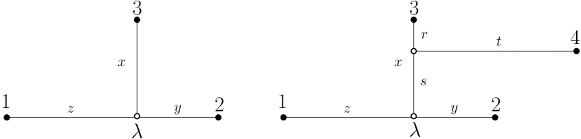
Figure 5: Left: tree of order $n=x+y+z+3$ with 3 leaves. Right: tree of order $n=x+y+z+t+4$ with 4 leaves

Clearly, $x$, $y$ and $z$ are strictly positive, since $\hat{B}$ satisfies property (1). Moreover, $x$, $y$ and $z$ are integers, since according to property (2), $a+b+c$ is an even integer, which means that integers $b+c-a$, $a+c-b$ and $a+b-c$ are also even. Hence, the distance matrix of the leaves of $T$ is $\hat{B}$. ∎

And now, the case $4\times 4$.

Lemma 22.

Let $\hat{B}$ be an integer metric dissimilarity matrix $4\times 4$ such that

1. $\hat{b}_{ij}<\hat{b}_{ik}+\hat{b}_{jk}$, for every distinct $i,j,k\in[4]$.

2. $\hat{b}_{ij}+\hat{b}_{ik}+\hat{b}_{jk}$ is even, for every distinct $i,j,k\in[4]$.

Then, $\hat{B}$ is the ${\cal L}(G)$-distance matrix $\hat{D}_{T}$ and thus it is additive.

Proof.

Let $\hat{B}$ be a dissimilarity matrix of order $4$ satisfying properties (1) and (2):

${\hat{B}}=\left(\begin{array}[]{rrrr}0&a&b&\alpha\cr a&0&c&\beta\cr b&c&0&\gamma\cr\alpha&\beta&\gamma&0\end{array}\right)$

We may assume, without loss of generality, that

$$a+\gamma\leq b+\beta\leq c+\alpha.$$

Consider the tree $T$ of order $n=x+y+z+t+4$ with 4 leaves displayed in Figure 5 (right).

If ${\hat{B}}={\hat{D}_{T}}$, then according to Lemma 21:

$$\left\{\begin{array}[]{rrrrrrrrrrrrrr}x=\frac{b+c-a}{2}\\ \\ y=\frac{a+c-b}{2}\\ \\ z=\frac{a+b-c}{2}\end{array}\right.$$

Moreover:

$$\left\{\begin{array}[]{rrrrrrrrrrrrrr}x=r+s\\ \\ \alpha=z+s+t\\ \\ \beta=y+s+t\\ \\ \gamma=r+t\end{array}\right.\Leftrightarrow\left\{\begin{array}[]{rrrrrrrrrrrrrr}r=\frac{x+z-\alpha+\gamma}{2}\\ \\ s=\frac{x-z+\alpha-\gamma}{2}\\ \\ t=\frac{-x-z+\alpha+\gamma}{2}\end{array}\right.\Leftrightarrow\left\{\begin{array}[]{rrrrrrrrrrrrrr}r=\frac{b-\alpha+\gamma}{2}\\ \\ s=\frac{c-a+\alpha-\gamma}{2}\\ \\ t=\frac{-b+\alpha+\gamma}{2}\end{array}\right.$$

Clearly, $r$ and $t$ are strictly positive, since $\hat{B}$ satisfies property (1). Moreover, $r$ and $t$ are integers, since according to property (2), $b+\alpha+\gamma$ is an even integer, which means that integers $b-\alpha+\gamma$ and $-b+\alpha+\gamma$ are both also even.

From the previous assumption 3.3 we derive that $s$ is non-negative. In addition, $s$ must be an integer, since $c-a+\alpha-\gamma=(b+\alpha-\gamma)-(a+b-c)$ is, according to property (2), either even or 0.

Hence, we have shown that ${\hat{B}}={\hat{D}_{T}}$, which means, according to Proposition 12, that ${\hat{B}}$ is an additive matrix. ∎

Remark 23.

Notice that, in the above proof, $a+\gamma=b+\beta=c+\alpha.$ if and only if $s=0$. Hence, in this case $T$ is a spider (see Figure 5 (right)).

At this moment, we are in disposition to prove the general result that determines which matrices are the $\partial(T)$-distance matrix of a tree $T$.

Theorem 24.

Let $\hat{B}_{\kappa}$ be an integer metric dissimilarity matrix of order $\kappa\geq 3$. Then, $\hat{B}_{\kappa}$ is the ${\cal L}(G)$-distance matrix $\hat{D}_{T}$ if and only if it is additive and

1. $\hat{b}_{ij}<\hat{b}_{ik}+\hat{b}_{jk}$, for every distinct $i,j,k\in[\kappa]$.

2. $\hat{b}_{ij}+\hat{b}_{ik}+\hat{b}_{jk}$ is even, for every distinct $i,j,k\in[\kappa]$.

Proof.

If for some tree $T$ with $\kappa$ leaves, $\hat{B}=\hat{D}_{T}$ is the distance matrix of the leaves of $T$, then it is a routine exercise to check that $\hat{B}$ is additive and satisfies properties (1) and (2).

To prove the converse, take an additive integer metric dissimilarity matrix $\hat{B}_{\kappa}$ of order $\kappa\geq 5$ satisfying properties (1) and (2). We distinguish cases.

Case 1.: For every 4-subset of indices $\{i,j,h,k\}\subseteq[\kappa]$,

$$\hat{b}_{ij}+\hat{b}_{hk}=\hat{b}_{ih}+\hat{b}_{jk}=\hat{b}_{ik}+\hat{b}_{jh}.$$

We claim that $\hat{B}_{\kappa}$ is the distance matrix $\hat{D}_{S_{\kappa}}$ of the set of leaves of a spider $S_{\kappa}$. To prove it, we proceed by induction on ${\kappa}\geq 4$. Notice that if $\kappa=4$, then according to Remark 23, our claim holds. Let $\kappa\geq 5$ and take the matrix $\hat{B}_{{\kappa}-1}$ obtained by deleting the last row and column of $\hat{B}_{\kappa}$.

By the inductive hypothesis, $\hat{B}_{{\kappa}-1}$ is the distance matrix $\hat{D}_{S_{\kappa-1}}$ of the set of leaves of a spider $S_{\kappa-1}$. Let ${\cal L}(S_{\kappa-1})=\{\ell_{1},\ldots,\ell_{\kappa-1}\}$ the set of leaves of $S_{\kappa-1}$, in such a way that for every $i,j\in[\kappa-1]$, $d(\ell_{i},\ell_{j})=[\hat{B}_{{\kappa}-1}]_{ij}$ Take the principal submatrix $\hat{B}_{4}$ of $\hat{B}_{{\kappa}}$ of order 4 obtained by considering the rows (and thus also the columns) in $\{1,2,3,\kappa\}$. According to Remark 23, there is a (unique) spider $S_{4}$ such that the distance matrix of its set of leaves $\{\ell_{1},\ell_{2},\ell_{3},\ell_{\kappa-1}\}$ is $\hat{B}_{4}$.

Let $S_{\kappa}$ the spider obtained by joining the spiders $S_{\kappa-1}$ and $S_{4}$. If ${\cal L}(S_{\kappa})=\{\ell_{1},\ldots,\ell_{\kappa-1},\ell_{\kappa}\}$, then for every $i,j\in[\kappa]$, $d(\ell_{i},\ell_{j})=\hat{b}_{ij}$, unless $4\leq i\leq\kappa-1$ and $j=\kappa$. Finally, if $4\leq i\leq\kappa-1$, then $d(\ell_{i},\ell_{\kappa})+d(\ell_{1},\ell_{2})=d(\ell_{1},\ell_{\kappa})+d(\ell_{i},\ell_{2})$. Thus, according to condition (3.3):

$$d(\ell_{i},\ell_{\kappa})=d(\ell_{1},\ell_{\kappa})+d(\ell_{i},\ell_{2})-d(\ell_{1},\ell_{2})=\hat{b}_{1\kappa}+\hat{b}_{i2}-\hat{b}_{12}=\hat{b}_{i\kappa}.$$

Case 2.: For some subset of indices $\{i,j,h,k\}\subseteq[\kappa]$,

$$\hat{b}_{ij}+\hat{b}_{hk}<\hat{b}_{ih}+\hat{b}_{jk}=\hat{b}_{ik}+\hat{b}_{jh}.$$

We proceed by induction on $\kappa\geq 3$. Cases $\kappa=3$ and $\kappa=4$ have been proved in Lemma 21 and Lemma 21, respectively. W.l.o.g., we assume that condition (3.3) holds for a 4-subset $\{1,j,h,\kappa\}$. Let $\hat{B}^{1}_{{\kappa}-1}$ and $\hat{B}^{\kappa}_{{\kappa}-1}$ be the matrices obtained by deleting row (and thus also column) 1 and $\kappa$ of $\hat{B}_{\kappa}$, respectively. Let $\hat{B}_{{\kappa}-2}$ be the matrix obtained by deleting rows (and thus also columns) 1 and $\kappa$ of $\hat{B}_{\kappa}$.

By the inductive hypothesis, $\hat{B}_{{\kappa}-2}$,$\hat{B}^{1}_{{\kappa}-1}$ and $\hat{B}^{\kappa}_{{\kappa}-1}$ are, respectively, the distance matrices of the set of leaves of three trees $T_{\kappa-2}$, $T^{1}_{\kappa-1}$ and $T^{\kappa}_{\kappa-1}$. Moreover, according to Theorem 19, $T_{\kappa-2}$ is a subtree of both $T^{1}_{\kappa-1}$ and $T^{\kappa}_{\kappa-1}$.

Let $T_{\kappa}$ the tree obtained by joining trees $T^{1}_{\kappa-1}$ and $T^{\kappa}_{\kappa-1}$. If ${\cal L}(T^{1}_{\kappa-1})=\{\ell_{2},\ldots,\ell_{\kappa}\}$, ${\cal L}(T^{\kappa}_{\kappa-1})=\{\ell_{1},\ldots,\ell_{\kappa-1}\}$ and ${\cal L}(T_{\kappa})=\{\ell_{1},\ldots,\ell_{\kappa-1},\ell_{\kappa}\}$, then for every $i,j\in[\kappa]$, $d(\ell_{i},\ell_{j})=\hat{b}_{ij}$, unless $i=1$ and $j=\kappa$. Finally, $d(\ell_{1},\ell_{\kappa})+d(\ell_{j},\ell_{h})=d(\ell_{1},\ell_{h})+d(\ell_{j},\ell_{\kappa})$. Thus, according to condition (3.3):

$$d(\ell_{1},\ell_{\kappa})=d(\ell_{1},\ell_{h})+d(\ell_{j},\ell_{\kappa})-d(\ell_{j},\ell_{h})=\hat{b}_{1h}+\hat{b}_{j\kappa}-\hat{b}_{jh}=\hat{b}_{1\kappa},$$

which means that $\hat{B}_{{\kappa}}$ is the distance matrix of $T_{\kappa}$. ∎

4 Reconstructing unicyclic graphs and their distance matrix

In this section, we depart from the comfortable and well-explored realm of trees to delve into a more rugged and less familiar territory: unicyclic graphs.

Although it would seem that the addition of a unique cycle does not change a lot the results, however this is certainly not the case. Firstly, there is not many literature research done on distance matrices of unicyclic graphs. Secondly, the boundary of a unicyclic graph not only contains its leaves but also the vertices of the cycle of degree 2. Although one can think that this is added information to the $\partial(G)$-distance matrix, the truth is that the reconstruction process turns out to be much more complicated.

This section is divided into two subsections: one dedicated to the procedure for knowing whether a matrix is the distance matrix of a unicyclic graph or not. The second one is dedicated to the process of reconstructing a unicyclic graph with $g\geq 5$ from its $\partial(G)$-distance matrix.

4.1 Distance matrices of a unicyclic graphs

In this subsection, our goal is to recognize whether a matrix is the distance matrix of a unicyclic graph. Unlike in the previous section, the procedure to check that condition is algorithmic. At each step, one can delete a leaf from the graph which is easily recognizable since it has only a one in its row and column. When there are no leaves, the resulting matrix should be one of a cycle (see Figure 6).

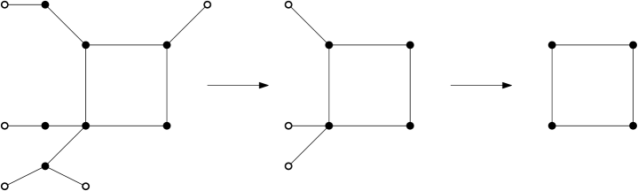
Figure 6: A graphical representation of the procedure to recognize algorithmically distance matrices of unicyclic graphs

Theorem 25.

A graph $G$ is unicyclic if and only the algorithm described above returns True.

Proof.

Let $D_{G}$ be the distance matrix of a graph $G$. Then, a row and a column with a unique one corresponds with a leaf in the graph $G$, and if we delete that row and column then the new matrix $D^{\prime}$ is the distance matrix of the graph $G^{\prime}$ obtained by deleting that leaf in $G$ (see Figure 6). Hence, if the final matrix of the above procedure is the distance matrix of a cycle, then it only remains to rebuild the graph to obtain a unicyclic graph. ∎

4.2 Reconstructing a unicyclic graph from its boundary distances

In this subsection, it is described the process of reconstructing a unicyclic graph from the distance matrix of its boundary. Given a unicyclic graph $G$ with $g\geq 5$, the procedure starts transforming the $\partial(G)$-distance matrix into a $\partial(G_{0})$-distance matrix where $G_{0}$ is also a unicyclic graph with the same girth as $G$ but without vertices of degree four nor vertices of degree three outside the cycle. Then, $G_{0}$ is reconstructed from its boundary distances and finally, the original $G$ is obtained.

According to Proposition 6, $\partial(G)={\cal L}(G)\cup{\cal U}(G)$. The next result gives us a procedure to distinguish the vertices of $\partial(G)$ with just the information provided by the matrix $\hat{D}_{G}$.

Lemma 26.

Let $G$ be a unicyclic graph with $g\geq 4$. Given the matrix $\hat{D}_{G}$, it is possible to distinguish the vertices in ${\cal L}(G)$ from the ones in ${\cal U}(G)$.

Proof.

First of all, if there is a one in a certain position of $\hat{D}_{G}$, then the two vertices of $\partial(G)$ at that position are adjacent, and so the vertices belong to ${\cal U}(G)$. Let $u\in{\cal U}(G)$ be one vertex not being in the above situation. Then, it has two neighbours with a branching tree having each of them at least one leaf $v_{1}$ and $v_{2}$. Remember that $v_{1},v_{2}\in{\cal L}(G)$. Since $g\geq 3$, the shortest path between $v_{1}$ and $v_{2}$ goes through $u$ and that can be detected in $\hat{D}_{G}$ by checking whether $d(v_{1},v_{2})=d(v_{1},u)+d(u,v_{2})$. Reciprocally, if three vertices $v_{1},v_{2},u\in\partial(G)$ verify that $d(v_{1},v_{2})=d(v_{1},u)+d(u,v_{2})$ and again $g\geq 3$, then $u$ is in the shortest path joining $v_{1}$ and $v_{2}$ and cannot be a leaf, and thus $u\in{\cal U}(G)$.

Once the vertices of ${\cal U}(G)$ have been located, by Proposition 6, ${\cal L}(G)=\partial(G)\setminus{\cal U}(G)$. ∎

Lemma 27.

Let $G$ be a unicyclic graph with $g\geq 5$. Let $\hat{D}_{G}$ be its $\partial(G)$-distance matrix. Given any vertex $x\in V(C_{g})$, $u\in{\cal L}(G)$ hangs out from $y\in V(C_{g})$, the antipodal vertex of $x$ if and only if $\forall v\in\partial(G),v\neq x,u$ and $d(u,x)+d(x,v)>d(u,v)$.

Proof.

On the contrary suppose that there exists $v\in\partial(G),v\neq x,u$ such that $d(u,x)+d(x,v)=d(u,v)$. Then, $x$ is in the shortest path between $u$ and $v$ and so, $u$ cannot hang out from the antipodal vertex of $x$.

Conversely, assume that $d(u,x)+d(x,v)>d(u,v)$ for any vertex $v$ in the boundary different from $u$ and $v$. Hence, $x$ is not in any shortest path $u-v$. Let $y\in V(C_{g})$ be the vertex from which hangs out $u$. For any $z\in V(C_{g})$, either $z\in\partial(G)$ or there exists $v$ hanging out from $z$. So $x$ is not in the shortest path between $y$ and any other vertex of the cycle, that is, $x$ and $y$ are antipodal.

Finally, note that all the distances can easily obtained from the matrix $\hat{D}_{G}$. ∎

We say that a unicyclic graph $G$ belongs to ${\cal G}_{0}$ if all its vertices of degree three lie on the cycle and it has no vertex of degree at least four. Otherwise, we say that $G$ is in ${\cal G}_{1}$. An important property of $G\in{\cal G}_{0}$ is that any vertex of its cycle belongs to ${\cal U}(G)$ or is joined with a path to exactly one leaf in ${\cal L}(G)$. Thus, for those unicyclic graphs, $|\partial(G)|=g$.

Lemma 28.

Let $G\in{\cal G}_{0}$ and let $u\in{\cal L}(G_{0})$. It is possible to determine the length of the path ending at $u$ only with the information provided in $\hat{D}_{G}$.

Proof.

Suppose that $u$ hangs out from the vertex $x$. Since $u\in{\cal L}(G)$, clearly $x\notin{\cal U}(G)$. We can delete $u$ from $G_{0}$, which in terms of the matrix $\hat{D}_{G}$ it means that the row and column corresponding to $u$ are reduced by one except the zero in the position $(u,u)$. Then, we can check if $x\in{\cal U}(G)$ using the procedure described in Lemma 26. If not, we continue deleting the vertices of the path between $u$ and $x$ until $x\in{\cal U}(G)$. The number of deleted vertices is the length of the path. ∎

Lemma 29.

Let $G$ a unicyclic graph with girth $g\geq 5$. Let $u\in{\cal L}(G)$ and let $S_{u}\subseteq V(G)$ be such that $u\in S_{u}$. Then, $S_{u}$ is the set of leaves of $T_{u}$ if and only if for all $w\in S_{u}$ there exists an integer $a_{w}$ such that $r(w|\partial(G)\setminus S_{u})=(a_{w},\stackrel{{\scriptstyle\kappa-|S_{u}|}}{{\ldots}},a_{w})+r(u|\partial(G)\setminus S_{u})$.

Proof.

Consider a certain leaf $u$ and the set $S_{u}$ of leaves in the same branching tree having $x\in V(G)$ as its branching-vertex, and $w\in S_{u}$. Then, we have that the distance between $u$ and $y\in\partial(G)\setminus S_{u}$ is $d(u,y)=d(u,x)+d(x,y)$ and since $w$ is in the same branching tree as $u$, the same occurs for $w$, i.e., $d(w,y)=d(w,x)+d(x,y)$. So, $d(w,y)-d(u,y)=d(w,x)-d(u,x)=a_{w}$ and therefore $d(w,y)=a_{w}+d(u,y)$. Note that $a_{w}$ does not depend of $y$ so it is the same integer for all the vertices in $\partial(G)\setminus S_{u}$.

Reciprocally, let $u$ be a leaf on $V(G)$ and $S_{u}$ is the set of leaves in the same branching tree as $u$. Let $w\in V(G)$ another leaf such that $r(w|\partial(G)\setminus S_{u})=(a_{w},\stackrel{{\scriptstyle\kappa-|S_{u}|}}{{\ldots}},a_{w})+r(u|\partial(G)\setminus S_{u})$. However, on the contrary, assume that $w\notin S_{u}$ which means that $w$ belongs to a different branching tree as $u$ with a different branching vertex $z$. There are three possibilities here: either $x$ and $z$ are adjacent or $d(x,z)=2$ or $d(x,z)>2$.

First, let us suppose that $x$ and $z$ are adjacent. Since $g\geq 5$, there exist two vertices in the cycle $x^{\prime}$ and $z^{\prime}$, respectively adjacent to $x$ and $z$. For the sake of simplicity, we might assume that $x^{\prime},z^{\prime}$ are not branching vertices. Otherwise, we can make the same reasoning with a leaf in each branching tree. Hence, we have the following distances:

$$d(u,x^{\prime})=d(u,x)+1;\qquad d(w,x^{\prime})=d(w,z)+2$$

$$d(u,z^{\prime})=d(u,x)+2;\qquad d(w,z^{\prime})=d(w,z)+1$$

According to the above, the value of $a_{w}$ would be $d(w,x^{\prime})-d(u,x^{\prime})=d(w,z)-d(u,x)+1$ and $d(w,z^{\prime})-d(u,z^{\prime})=d(w,z)-d(u,x)-1$ which is clearly impossible.

On the other hand, let us suppose that $d(x,z)>2$, i.e., there exist at least two intermediate vertices $y$ and $y^{\prime}$ in the shortest path between $x$ and $z$ being $y$ closer to $x$ than to $z$. Again, for simplicity, we can assume that neither $y$ nor $y^{\prime}$ are branching vertices since otherwise we can reasoning with a leaf hanging out from each of them. Then, $d(w,y)-d(u,y)=d(w,z)+d(z,y^{\prime})+d(y^{\prime},y)-d(u,x)-d(x,y)$ and $d(w,y^{\prime})-d(u,y^{\prime})=d(w,z)+d(z,y^{\prime})-d(u,x)-d(x,y)-d(y,y^{\prime})$ which cannot be equal unless $y=y^{\prime}$ and $d(x,z)=2$ which is not the case.

Finally, suppose that $d(x,z)=2$ so there exists only one intermediate vertex $y$ in the shortest path between $x$ and $z$. For the same reasons as above, we may assume that $y$ is not a branching vertex. Since $g\geq 5$, there is another vertex in the cycle $x^{\prime}$ adjacent to $x$. Then, $d(w,y)-d(u,y)=d(w,z)-d(u,x)$ and at the same time $d(w,x^{\prime})-d(u,x^{\prime})=d(w,z)+d(z,x^{\prime})-d(u,x)-1$ and those two quantities are only equal if $d(z,x^{\prime})=1$ which is not possible since $g\geq 5$. Thus, in any case we have reached a contradiction and so necessarily $w\in S_{u}$. ∎

Note that the hypothesis $g\geq 5$ is necessary as otherwise we could have the graph of Figure 7 that does not verify Lemma 29.

Figure 7: A graph of girth $g=4$ not verifying the condition of Lemma 29

In the following, we are going to show that beginning with the matrix $\hat{D}_{G}$ of a graph $G\in{\cal G}_{1}$, we can construct the matrix $\hat{D}_{G_{0}}$ of a graph $G_{0}\in{\cal G}_{0}$ and some extra information, and that the process can be reversed to obtain the original graph.

Algorithm 2 ${\cal G}_{1}$ to ${\cal G}_{0}$

1:A matrix $\hat{D}_{G}$ of a graph $G\in{\cal G}_{1}$ with $g\geq 5$.

2:The matrix $\hat{D}_{G_{0}}$ of a graph $G_{0}\in{\cal G}_{0}$, a list of matrices $\{M(u)\}_{u\in U}$ and a list of vectors $\{L(u)\}_{u\in U}$ where $u\in U\subseteq{\cal L}(G)$.

3:Mark all the leaves of $\partial(G)$ following the procedure described in Lemma 26;

4:Separate all the leaves into sets $S_{u}$ by using the criteria of Lemma 29;

5:Denote $U$ as the set of vertex representatives $u$ with a set $S_{u}$;

6:for any $u\in U$ do

7:     Let $M(u)$ be the submatrix of $\hat{D}_{G}$ with vertices in $S_{u}$;

8:     Find the distance $a$ from $u$ to its branching vertex $x$ as it is described in Lemma 28 and add $a$ to $L(u)$;

9:     for any $w\in S_{u}$ and $w\neq u$ do

10:         Add to $L(u)$ the distance from $w$ to $x$ according to Lemma 28;

11:         Delete from $\hat{D}_{G}$ the row and column corresponding to $w$;

12:     end for

13:end for

14:return $\hat{D}_{G}$ as $\hat{D}_{G_{0}}$ and the lists $\{M(u)\}_{u\in U}$ and $\{L(u)\}_{u\in U}$.

Lemma 30.

Given $\hat{D}_{G}$ of a unicyclic graph $G$, Algorithm 2 returns $\hat{D}_{G_{0}}$ of a graph $G_{0}$ of type ${\cal G}_{0}$ with the same girth as $G$ and a leaf for each branching tree in $G$.

Proof.

First of all, the algorithm only deals with leaves of $G$, and only deletes leaves from $\hat{D}_{G}$. So the vertices of the cycle are unchanged and the girth of $G_{0}$ is the same as the one of $G$.

On the other hand, we detect all the leaves in the same tree as $u$ by using the Lemma 29 and delete them except $u$. ∎

Algorithm 3 ${\cal G}_{0}$ to ${\cal G}_{1}$

A $G_{0}\in{\cal G}_{0}$ with $g\geq 5$, a list of matrices $\{M(u)\}_{u\in U}$ and a list of vectors $\{L(u)\}_{u\in U}$ obtained from Algorithm 2.

An isomorphic graph $G\in{\cal G}_{1}$ to the original one.

for each $u$ in $U$ do

     Find $x$ the branching vertex of $u$ in $G_{0}$;

     With the information of $M(u)$ and $L(u)$ construct the matrix $\hat{D}_{T_{u}}$ that corresponds with the tree $T_{u}$ containing the vertices in $S_{u}$ as leaves;

     Apply Algorithm 1 to $\hat{D}_{T_{u}}$;

     Substitute the path $x-u$ in $G_{0}$ by the subtree $T_{u}$;

end for

return $G_{0}$ as $G$.

Lemma 31.

Given $\hat{D}_{G_{0}}$ of a unicyclic graph $G_{0}\in{\cal G}_{0}$ and the lists $\{M(u)\}_{u\in U}$ and $\{L(u)\}_{u\in U}$, obtained by Algorithm 2 from a unicyclic graph $G\in{\cal G}_{1}$, the Algorithm 3 returns an isomorphic graph as $G$.

Proof.

Since the procedure does not alter the cycle and it substitutes any path by the original branching tree, the final graph would be isomorphic to the original one. ∎

Algorithm 4 Reconstructing ${\cal G}_{0}$. Part I

1:A matrix $\hat{D}_{G_{0}}$ of a graph $G_{0}\in{\cal G}_{0}$ with $g\geq 5$.

2:The graph $G_{0}$.

3:Let $G$ be a cycle $C_{g}$ of length $g$, the order $g$ of $\hat{D}_{G_{0}}$; Find ${\cal U}(G_{0})$ and ${\cal L}(G_{0})$ as in Lemma 26;

4:if $g$ is odd then

5:     if there is an antipodal pair $x_{1},x_{2}\in{\cal U}(G_{0})$ then

6:         Mark them in $G$;

7:     else if ${\cal U}(G_{0})=\emptyset$ then

8:         Let $u\in{\cal L}(G_{0})$; Find the length $a$ as in Lemma 28;

9:         Add to $G$ the path $u-x_{1}$ length $a$ where $x_{1}\in V(C_{g})$;

10:         Add $x_{1}$ to $\hat{D}_{G_{0}}$ such that $\hat{D}_{G_{0}}(x_{1},y)=\hat{D}_{G_{0}}(y,x_{1})=\hat{D}_{G_{0}}(u,y)-d_{G}(x_{1},u)$ for all $y$ in $\hat{D}_{G_{0}}$;

11:     else [$|{\cal U}(G_{0})|\geq 1$]

12:         Let $x_{1}\in{\cal U}(G_{0})$;

13:         Let $x_{2}$ and $v$ be respectively an antipodal vertex in $C_{g}$ and an antipodal leaf to $x_{1}\in{\cal U}(G_{0})$ as shown in Lemma 27;

14:         Add the path $v-x_{2}$ of length $\hat{D}_{G_{0}}(x_{1},v)-d_{G}(x_{1},x_{2})$ to $G$;

15:         Add $x_{2}$ to $\hat{D}_{G_{0}}$ and assign $\hat{D}_{G_{0}}(x_{2},y)=\hat{D}_{G_{0}}(y,x_{2})=\hat{D}_{G_{0}}(v,y)-d_{G}(x_{2},v)$ for all $y$ in $\hat{D}_{G_{0}}$;

16:     end if

17:else [$g$ is even]

18:     if $x_{1},x_{2},x_{3}\in{\cal U}(G_{0})$ is a geodesic triple then

19:         Mark them in $G$ at distances $\hat{D}_{G_{0}}(x_{1},x_{2}),\hat{D}_{G_{0}}(x_{2},x_{3})$ and $\hat{D}_{G_{0}}(x_{3},x_{1})$;

20:     else if $|{\cal U}(G_{0})|=0$ then

21:         Pick $u\in{\cal L}(G_{0})$ and determine $a$ as in Lemma 28;

22:         Add the path $u-x_{1}$ of length $a$ to $G$ where $x_{1}$ is any vertex of $C_{g}$;

23:         Add $x_{1}$ to $\hat{D}_{G_{0}}$ where $\hat{D}_{G_{0}}(x_{1},y)=\hat{D}_{G_{0}}(y,x_{1})=\hat{D}_{G_{0}}(u,y)-d_{G}(x_{1},u)$ for all $y$ in $\hat{D}_{G_{0}}$;

24:     else [$|{\cal U}(G_{0})|\geq 1$]

25:         Let $x_{1}\in{\cal U}(G_{0})$;

26:         if $|{\cal U}(G_{0})|=1$ then

27:              Let $x_{2}$ be the antipodal vertex to $x_{1}$ in $C_{g}$ and find an antipodal leaf $v$ to $x_{1}$ according to Lemma 27;

28:              Add the path $v-x_{2}$ of length $\hat{D}_{G_{0}}(x_{1},v)-d_{G}(x_{1},x_{2})$ to $G$;

29:              Add $x_{2}$ to $\hat{D}_{G_{0}}$ such that $\hat{D}_{G_{0}}(x_{2},y)=\hat{D}_{G_{0}}(y,x_{2})=\hat{D}_{G_{0}}(v,y)-d_{G}(x_{2},v)$ for all $y$ in $\hat{D}_{G_{0}}$;

30:         else [$|{\cal U}(G_{0})|\geq 2$]

31:              $x_{2}\in{\cal U}(G_{0})$;

32:              Let $w\in{\cal L}(G_{0})\setminus\{u,v\}$ and find one vertex $x_{3}$ in $V(C_{g})$ such that $r(v|\{x_{1},x_{2}\})=(a,a)+r(x_{3}|\{x_{1},x_{2}\})$; Add the path $w-x_{3}$ of length $a$ to $G$;

33:              Add $x_{3}$ to $\hat{D}_{G_{0}}$ such that $\hat{D}_{G_{0}}(x_{3},y)=\hat{D}_{G_{0}}(y,x_{3})=\hat{D}_{G_{0}}(w,y)-d_{G}(x_{3},w)$ for all $y$ in $\hat{D}_{G_{0}}$;

34:         end if

35:     end if

36:end if

Algorithm 5 Reconstructing ${\cal G}_{0}$. Part II

37:if $g$ is odd then

38:     Assign to every vertex $x$ in $V(C_{g})$ the coordinates $r(x|\{x_{1},x_{2}\})$;

39:     for any vertex $u\in{\cal L}(G_{0})$ not yet in $G$ do

40:         Find the vertex $x\in V(C_{g})$ such that $r(u|\{x_{1},x_{2}\})=(a,a)+r(x|\{x_{1},x_{2}\})$ and add the path $u-x$ of length $a$ to $G$;

41:     end for

42:else [$g$ is even]

43:     Assign to every vertex $x$ in $V(C_{g})$ the coordinates $r(x|\{x_{1},x_{2},x_{3}\})$;

44:     for any vertex $u\in{\cal L}(G_{0})$ not yet in $G$ do

45:         Find the vertex $x\in V(C_{g})$ such that $r(u|\{x_{1},x_{2},x_{3}\})=(a,a,a)+r(x|\{x_{1},x_{2},x_{3}\})$ and add the path $u-x$ of length $a$ to $G$;

46:     end for

47:end if

48:return $G$.

Lemma 32.

In the previous algorithm, $\{x_{1},x_{2}\}$ when $g$ is odd, and $\{x_{1},x_{2},x_{3}\}$, when $g$ is even, is a doubly resolving set for the vertices of the cycle of $G$.

Proof.

In the case $g$ odd, $x_{2}$ is an antipodal vertex of $x_{1}$ which guarantees that both of them form a doubly resolving set.

When $g$ is even, $x_{1},x_{2}$ and $x_{3}$ are a geodesic triple and again, that is enough for being a doubly resolving set. ∎

Theorem 33.

Beginning with the distance matrix $\hat{D}_{G_{0}}$ of the boundary vertices of a unicyclic graph $G_{0}\in{\cal G}_{0}$, Algorithm 4 obtains an isomorphic graph to $G_{0}$ in $O(n^{2})$.

Proof.

The first part of the algorithm consists of obtaining a doubly resolving set of the vertices of the boundary as it is stated in Lemma 32. In the second part, any path ending in a leaf is added to the final graph. The complexity is given by several steps that run in time $O(n^{2})$, for instance 39 and 44. ∎

Theorem 34.

Let $G$ be a unicyclic graph on $n$ vertices and let $\partial(G)=\{\ell_{1},\ldots,\ell_{\kappa}\}$. Then, $G$ is uniquely determined by the $\partial(G)$-distance matrix $\hat{D}_{G}$.

Proof.

Given the distance matrix $\hat{D}_{G}$ of the boundary vertices in a unicyclic graph $G$, we can apply Algorithm 2 to obtain the distance matrix $\hat{D}_{G_{0}}$ of the boundary of a new graph $G_{0}$, then Algorithm 4 to get the graph $G_{0}$, and finally Algorithm 3 to reconstruct the original graph $G$. ∎

5 Conclusions and Further work

In [22], it was firstly implicitly mentioned that a resolving set $S$ of a graph $G=(V,E)$ is strong resolving if and only if the distance matrix $D_{S,V}$ uniquely determines the graph $G$ (see Theorem 9). On the other hand, in [21] it was proved that the boundary $\partial(G)$ of every graph $G$ is a strong resolving set (see Proposition 4).

Mainly having in mind this pair of results, we have presented in Section 2 the following conjecture.

Conjecture 35.

Let $\hat{B}$ a metric dissimilarity matrix of order $\kappa$. Let $G=([n],E)$ be a graph such that $\hat{D}_{G}=\hat{B}$. If $G^{\prime}=([n],E^{\prime})$ is a graph such that $\hat{D}_{G^{\prime}}=\hat{B}$, then $G$ and $G^{\prime}$ are isomorphic.

In Sections 3 and 4, we have proved this conjecture for trees and unicyclic graphs, respectively, and we have provided algorithms to recognize trees and unicyclic graphs.

In addition, in Section 3, we have been able to characterize, for trees, both the distance matrix $D_{T}$ and the $\partial(T)$-distance matrix $\hat{D}_{T}$ (see Theorems 18, 19 and 24).

We conclude with a list of suggested open problems.

Open Problem 1:

Characterizing distance matrices of unicyclic graphs in a similar way as it has been done for trees in this work.

Open Problem 2:

Characterizing the distance matrix of the boundary of a unicyclic graph $G$ belonging to ${\cal G}_{0}$.

Open Problem 3:

Characterizing the distance matrix of the boundary of a unicyclic graph $G$ belonging to ${\cal G}_{1}$.

Open Problem 4:

Checking Conjecture 35 for Block graphs.

Open Problem 5:

Checking Conjecture 35 for Cactus graphs.

Open Problem 6:

Checking Conjecture 35 for Block-cactus graphs.

Open Problem 7:

Proving (or disproving) Conjecture 35 for Split graphs of diameter 3.

Open Problem 8:

Proving (or disproving) Conjecture 35 for Ptolemaic graphs.

6 Acknowledgements

This work is partially supported by Junta de Andalucía group AGR-199 and Universitat Politècnica de Catalunya under funds AGRUP-UPC.

References

- [1] Ahmed, M., Wenk, C.: Constructing street networks from GPS trajectories. In: Epstein, L., Ferragina, P. (eds.) ESA 2012. LNCS 7701, 60–71. Springer, Heidelberg (2012). https://doi.org/10.1007/978-3-642-33090-27
- [2] Brandes, U., Cornelsen, S.: Phylogenetic graph models beyond trees. Discrete Appl. Math. 157(10), 2361–2369 (2009)
- [3] Buneman, P.: A note on the metric properties of trees. J. Combinatorial Theory Ser. B, 17, 48–50 (1974). https//doi.org/10.1016/0095-8956(74)90047-1
- [4] Cáceres, J., Hernando, C., Mora, M., Pelayo, I. M., Puertas, M. L., Seara, C.: On geodetic sets formed by boundary vertices. Discrete Math. 306(2), 188–198 (2006). https://doi.org/ 10.1016/j.disc.2005.12.012
- [5] Cáceres, J., Hernando, C., Mora, M., Pelayo, I. M., Puertas, M. L., Seara, C., Wood, D. R.: On the metric dimension of Cartesian products of graphs. SIAM J. Discrete Math. 21(2), 423–441 (2007). https://doi.org/10.1137/050641867
- [6] Cáceres, J., Pelayo, I. M.: Metric Locations in Pseudotrees: A survey and new results. Submitted (2023)
- [7] Chartrand, G., Erwin, D., Johns, G. L., Zhang, P.: Boundary vertices in graphs. Discrete Math. 263(1-3), 25–34 (2003). https://doi.org/10.1016/S0012-365X(02)00567-8
- [8] Chartrand, G., Lesniak, L., Zhang, P.: Graphs and digraphs. CRC Press, Boca Raton, FL, (2016). https://doi.org/10.1201/b19731
- [9] Day, T.K., Wang, J., Wang, Y.: Graph reconstruction by discrete Moore theory. In: Proceedings of the 34th International Symposium on Computational Geometry. Leibniz International Proceedings in Informatics (LIPIcs) 99, 31:1–31:15 (2018). https://doi.org/10.4230/LIPIcs.SoCG.2018.31
- [10] Graham, R. L., Pollack, H. O.: On the addressing problem for loop switching. Bell Syst. Tech. J. 50, 2495–2519 (1971)
- [11] Hakimi, S. L., Yau, S. S.: Distance matrix of a graph and its realizability. Quart. Appl. Math. 22, 305–317 (1965). https://doi.org/10.1090/qam/184873
- [12] Hasegawa, Y., Saito, A.: Graphs with small boundary. Discrete Math. 307(14), 1801–1807 (2007). https://doi.org/10.1016/j.disc.2006.09.028
- [13] Hernando, C., Mora, M., Pelayo, I. M., Seara, C.: Some structural, metric and convex properties of the boundary of a graph. Ars Combin. 109, 267–283 (2013)
- [14] Howorka, E.: On metric properties of certain clique graphs. J. Combin. Theory Ser. B 27(1), 67–74 (1979). https://doi.org/10.1016/0095-8956(79)90069-8
- [15] Kannan, S., Mathieu, C., Zhou, H.: Graph reconstruction and verification. ACM Trans. Algorithms 14(4), 1–30 (2018).https://doi.org/10.1145/3199606
- [16] Kelly, P.J.: On Isometric Transformations. Ph.D. thesis, University of Wisconsin (1942)
- [17] Kuziak, D.: The strong resolving graph and the strong metric dimension of cactus graphs. Mathematics 8, 1266 (2020). https://doi.org/10.3390/math8081266
- [18] Lin, H., Liu, R., Lu, X.: The inertia and energy of the distance matrix of a connected graph. Linear Algebra Appl. 467, 29–39 (2015). https://doi.org/10.1016/j.laa.2014.10.045
- [19] Mossel, E., Ross, N.: Shotgun assembly of labeled graphs. IEEE Trans. Netw. Sci. Eng. 6(2), 145–157 (2017). https://doi.org/10.1109/TNSE.2017.2776913
- [20] Oellermann, O. R., Peters-Fransen, J.: The strong metric dimension of graphs and digraphs. Discrete Appl. Math. 155(3), 356–364 (2007). https://doi.org/10.1016/j.dam.2006.06.009
- [21] Rodríguez-Velázquez, J. A., Yero, I. G., Kuziak, D., Oellermann, O. R.: On the strong metric dimension of Cartesian and direct products of graphs. Discrete Math. 335, 8–19 (2014). https://doi.org/10.1016/j.disc.2014.06.023
- [22] Se̋bo, A., Tannier, E.: On metric generators of graphs. Math. Oper. Res. 29(2), 383–393 (2004). https://doi.org/10.1287/moor.1030.0070
- [23] Simões Pereira, J. M. S.: A note on the tree realizability of a distance matrix. J. Combinatorial Theory 6, 303–310 (1969)
- [24] Slater, P. J.: Leaves of trees. Congr. Numer. 14, 549–559 (1975)
- [25] Steinerberger, S.: The boundary of a graph and its isoperimetric inequality. Discrete Appl. Math. 338, 125–134 (2023). https://doi.org/10.1016/j.dam.2023.05.026
- [26] Ulam, S.M.: A Collection of Mathematical Problems. In:Interscience Tracts in Pure and Applied Mathematics 8. Interscience Publishers (1960)
- [27] Waterman, M. S., Smith, T. F., Singh, M., Beyer, W. A.: Additive evolutionary trees. J. Theoret. Biol. 64(2), 199–213 (1977). https://doi.org/10.1016/0022-5193(77)90351-4