MnLargeSymbols’164 MnLargeSymbols’171
Elastic Curves with Variable Bending Stiffness
Abstract.
We study stationary points of the bending energy of curves subject to constraints on the arc-length and total torsion while simultaneously allowing for a variable bending stiffness along the arc-length of the curve. Physically, this can be understood as a model for an elastic wire with isotropic cross-section of varying thickness. We derive the corresponding Euler-Lagrange equations for variations that are compactly supported away from the end points thus obtaining characterizations for elastic curves with variable bending stiffness. Moreover, we provide a collection of alternative characterizations, e.g., in terms of the curvature function. Adding to numerous known results relating elastic curves to dynamics, we establish connections between elastic curves with variable bending stiffness and damped pendulums and the flow of vortex filaments with finite thickness.
MSC (2020). Primary 53A04; Secondary 53C21, 53C42, 53C44, 74K10, 74B20.
Keywords. Elastic curves, variable bending stiffness, Euler-Lagrange equations, pendulum equation, vortex filament flow.
1. Introduction
In mathematics and the natural sciences alike, one-dimensional flexible structures have diverse applications ranging from architectural beams to molecular modeling. Despite a longstanding history of research, they remain a prominent research topic.
Stationary points of the so-called bending energy on the space of curves , are used to model, e.g., the bent shapes of an ideal infinitesimally thin elastic rod (without stretching) [33]. This classical problem dates back to the 13th century and the current state of knowledge is still largely based on the work of mathematical pioneers such as Bernoulli and Euler [33]. Only the rigorous definition of the curvature of a planar curve paved the way for their seminal work, culminating in the characterization of plane elastic curves as the stationary points of the energy functional ([14], Fig. 1)
It was soon discovered that planar elastic curves relate to a variety of other phenomena in the natural sciences [33]. For regular space curves the bending energy is given by
Kirchhoff realized the importance of torsion and related the generalized the problem of elastic curves in three-dimensions with the dynamics of a spinning top [28]. For more in depths reviews of the history of elastic curves see, e.g., [33, 22].
Elastic curves have broad utility, praised for their aesthetics and practicality. They are used as models for plant stems [20, 21], DNA strands [2, 16, 38], for preventing kinks and loops in marine cables [23, 50], guiding track layouts, and even in medical applications such as surgical wires [47]. In design and computer graphics they serve as decorative elements in [53] and play a crucial role in simulation software, particularly in complex tasks like hair simulation [11, 48, 5, 29]. The discretization [3, 7] and efforts to approximate elastic curves with computationally more efficient splines [8] form a crucial facet of current research.
Elastic curves’ energy-minimizing characteristics and their direct link to material bending make them appealing for architecture and modern fabrication. Fabrication-aware design and cost-effective manufacturing processes, such as active bending [34], leverage certain material properties. Bending and twisting, once challenges, are now utilized as tools, reflecting a shift “from failure to function” [1]. This shift has amplified interest in the “inverse problem,” where researchers seek to control material parameters to achieve specific shapes, a significant facet of elasticity research [6, 24, 25]. Economic considerations, including ease of manufacturing, transportation, and installation for curved shapes, are pivotal in architecture and fabrication. Techniques like active bending offer numerous advantages [34], and morphing structures leverage bending to attain or modify their desired shapes [35].
Various surface design methods extend elastic curve theory to approximate -dimensional curved shapes using networks of single rods. These approaches are instrumental in modern fabrication, including rod meshes and gridshells [1, 49, 42], and deployable structures [41, 44]. Another modeling technique combines elastic curves with minimal surfaces, as seen in Plateau surfaces [18, 43]. In this context, the energy of the whole system depends on the energy of the bounding elastic curve [4, 17].
On a theoretical level, Langer and Singer made significant contributions[30, 31], among other results elucidating the connection between Kirchhoff rods and solitons, leading to integrable Hamiltonian systems, building upon Hasimoto’s vortex filament flow analogy [26]. Today, elastic curves are known to share an intricate relationship with many dynamical systems arising from natural phenomena. For example, they are exactly those whose evolution under the vortex-filament flow is (up to reprarametrization) a rigid motion. Moreover, they can be described as the orbits of charged particles moving in a magnetic field. [13, 45]. The tangent vectors of stationary points of the bending energy with a sole length-constraint, so-called torsion free elastic curves, are known to relate to the motion of the axis of a spinning top [28] and solve the pendulum equation [45].
Only recently, Bretel and McCarthy established that the space of equilibrium states of a flexible wire anchored at its endpoints is a finite-dimensional manifold [10]. Also closed curves and “elastic knots” offer a range of interesting results, be it theoretical [51, 32] or practical [52].
Complementing previous work, our main focus is on space curves that exhibit an isotropic resistance to bending which may vary along the arc-length of the curve. We will refer to such a curve as a curve with variable bending stiffness. From a physical viewpoint, these elastic curves model idealized elastic rods with circular cross-section of varying diameter. The study of curves with additional free parameters such as thickness has become an important task in the natural sciences, as they appear as key structural motifs in a variety of contexts (see, e.g., [36, 19, 12, 37] and references therein). The variable bending stiffness is formalized by weighting the integrand of the bending energy by a strictly positive function
which represents the bending stiffness of the curve along the arc-length. Consequently, the bending energy takes the form
| (1.1) |
Previous investigations on this topic focused on closed planar elastic curves whose stiffness depends on an additional density variable [27, 9], or developed computational methods and applications [40, 24, 25].
Inspired by [25], who considered a significantly larger configuration space allowing for anisotropic cross sections and focused on the inverse problem, on a conceptual level, our approach differs significantly from previous work. We consider a somewhat more restrictive variational problem asking for isotropic cross-sections, thus remaining closer to the classical problem. However, similar to the -dimensional case, where the step from a “bending beam” to solving the formal Euler-Lagrange equations reveals considerably more interesting curves, we obtain a large number of novel elastic curves with variable bending stiffness. Most importantly, we observe connections to dynamical systems, which are already well established in the classical setup. Further investigation of these aspects seems to be an exciting avenue for future research on their own.
1.1. Structure of the Article
The article is structured as follows: in Section 1 we outline related work and place our own work in the context of existing literature. In Section 2 we fix the notation and introduce preliminary definitions and theorems for further discussion. The Euler-Lagrange equations for the problems of elastic curves with variable bending stiffness subject to constrained arc-length and/or total torsion are derived in Section 3. The Euler-Lagrange equations can be reformulated into equivalent characterizations, which we do in Section 4, while in Section 4.1 we express them in terms of the curvature function. Last, in Section 5, we investigate how established connections to dynamical systems, such as physical pendulums or the vortex filament flow, generalize to our novel setup.
2. Preliminaries
In this section, we briefly introduce preliminaries and fix the notation used throughout the article. We will denote the set of all smooth functions from an interval into by . For our purposes we always assume that . A curve is a map with . Denoting the standard Euclidean norm on by , we refer to as the arc-length of and the length of a curve is given by
A curve is said to be parameterized by arc-length if . The derivative of a function with respect to the arc-length of is defined as . In particular, the unit tangent vector field of a curve is given by .
2.1. The Bending Energy with Bending Stiffness
The norm of the derivative with respect to the arc-length of the unit tangent vector, measures the failure of the curve to be a straight line segment. Integrating the squared norm of this error over the arc-length therefore measures how much the curve bends in space. Consequently the bending energy of a curve is given by
| (2.1) |
Historically, the motivation for studying elastic curves has been to gain a better understanding of the shapes that a thin elastic cable takes when the end points are held fixed. We extend the theory in the sense that we do not assume for a cable of constant thickness, but allow for varying thickness which is accounted for by weighting the bending energy density along the curve.
Definition 2.1 (Bending energy with bending stiffness).
The bending energy of a curve with bending stiffness is given by
| (2.2) |
2.2. The Total Torsion of a Space Curve
A normal field satisfies and is said to be parallel if for some . By solving a corresponding initial value problem any normal vector to a curve can be extended to a unique parallel normal field along [45, Thm. 4.3].
Definition 2.2.
For a curve let be a pair of unit vectors. Then, the total torsion of the curve with respect to is the unique angle such that
| (2.3) |
where is the unique vector obtained from a parallel transport of along .
2.3. Variations of Curves, Length and Total Torsion
In the forthcoming sections we will define a hierarchy of “elastic curves” as stationary points of bending energy with bending stiffness (2.2) under perturbations with constraint length, arc-length or total torsion. For and , a smooth variation of is a one-parameter family
| (2.4) |
where and which satisfies and such that the map
is smooth. Given a smooth variation of a map , also , as well as , where is defined as
are smooth. To simplify the notation, we will omit the index when we evaluate at time and write . Moreover, we denote the variation of a smooth functional on corresponding to a smooth variation with variational vector field by
Our main object of interest are smooth variations of curves, for which we refer to
| (2.5) |
as the variational vector field. A variation of a curve is said to have compact support in the interior of if there is such that for all it holds that . We denote the vector space of functions with support in the interior of by and treat variations and corresponding variational vector fields as synonyms. Some useful identities are collected in
Lemma 2.3 ([45, Ch. 2]).
Let and . Then,
-
(1)
.
-
(2)
.
-
(3)
.
Theorem 2.4.
Let and . Then,
Proof.
We can also compute the variational gradient of the total torsion.
Theorem 2.5.
Let and . Then, independent of the choice of it holds that
| (2.6) |
Proof.
This follows from restricting [45, Thm. 5.3] to variations in . ∎
3. Euler-Lagrange Equations
With all necessary preliminaries in place, we start this section with computing the variational formula of the bending energy with bending stiffness (2.2) for a curve with bending stiffness under a general variation .
Theorem 3.1 (Variational formula for the bending energy).
Let with bending stiffness . Then, the variation of the bending energy with bending stiffness (2.2) with respect to is given by
| (3.1) |
where
| (3.2) |
Proof.
First of all the variation of Bending Energy with bending stiffness is given as:
We split the integral just to keep computations more clear. Using integration by parts we obtain
Similarly, for the second integral we get
Adding the two results yields the claim. ∎
3.1. Free Elastic Curves with Bending Stiffness
Theorem 3.1 bears several significant implications. When we imagine an (initially perfectly straight) elastic wire, it naturally wants to minimizes its bending energy. Holding a piece of such wire in our hands, we fix its end-points (and in fact even its tangent directions at the end points). Therefore, from a physical point of view, it is reasonable to restrict our attention to variations of (2.2) with compact support in the interior of .
Already in classical theory, free elastic curves111i.e., unconstrained stationary points of the bending energy take on a special role because, up to scaling and positioning, there is only one such curve. It turns out that this is true even in our generalized setup. Our results in Section 4.1 imply that there are no free elastic curves whose bending stiffness is non-constant.
Theorem 3.2.
Free elastic curves have constant bending stiffness.
3.2. Torsion-Free Elastic Curves with Bending Stiffness
Our investigations are inspired by deformations of physical rods or cables, possibly with non-uniform thickness distribution. We assume for the thickness to be prescribed along the arc length of the cable.
To incorporate this assumption into our model we constrain the set of admissible variations to the arc-length parameterized curves. By standard means of calculus of variations, this can be achieved by introducing a suitable Lagrange multiplier [46, 54]. More specifically, a curve with bending stiffness is a stationary point of (2.2) subject to the pointwise constraint
if and only if there exists a function such that is a stationary point of
| (3.3) |
Remark 3.3.
Note that the arc-length constraint is in fact appropriate when dealing with non-uniform bending stiffness. Unlike as for a balloon animal, to mimic the behavior of a physical cable, the thickness shall not be redistributed along the curve. A sole constraint on the length does not rule out such scenarios, though clearly the arc-length constraint also automatically constraints the length of the curve .
Definition 3.4 (Torsion-free elastic curve with bending stiffness).
An arc-length parametrized curve with bending stiffness is torsion-free elastic with bending stiffness if it is a critical point of the energy in Eq. (2.2) under all variations constraining the arc-length of the curve.
Theorem 3.5.
A curve with bending stiffness is a torsion-free elastic curve if and only if there is a such that
In terms of the unit tangent field this can be expressed by
or equivalently, in terms of ,
If the bending stiffness is constant, also the the Lagrange multiplier becomes a constant to which we refer to as tension and denote it by .
Proof.
Taking the time derivative of the augmented functional in Eq. (3.3) and using integration by parts we compute
Note that the boundary terms vanish since we consider variations and the claim follows. ∎
3.3. Elastic Curves with Bending Stiffness
In this section we will restrict our attention to curves in . As outlined in Section 1, Kirchhoff established torsion as an important parameter when modeling the shapes of elastic wires. We will refer to stationary points of (2.2) under arc-length preserving variations and with constrained total torsion (Definition 2.2) as elastic curves222They are also known as Kirchhoff elastica..
Definition 3.6 (Elastic curve with bending stiffness).
A curve with bending stiffness is said to be an elastic curve if it is a critical point of the energy in Eq. (2.2) under all variations constraining the arc-length and total torsion of the curve.
We can again derive the Euler-Lagrange equation characterizing elastic curves by introducing a suitable Lagrange multiplier constraining the total torsion (Theorem 2.5). For holonomic constraints such as fixed length, or total torsion, the Lagrange multipliers are in fact constants [45, Sec. 2].
Theorem 3.7.
A curve with bending stiffness is an elastic curve if and only if there is a smooth function and a constant such that
In terms of the unit tangent field this can be expressed by
or equivalently, in terms of ,
4. Equivalent Charecterizations
In this section we derive equivalent characterizations of the elastic curves we derived in the preceding sections. More specifically, we derive analogs of a list of statements which, for the classical case with constant bending-stiffness, relate elastic curves to dynamical systems such as spinning tops, pendulums, the non-linear Schrödinger equation and the vortex-filament flow [13, 45].
Theorem 4.1.
For an arc-length parameterized curve with unit tangent vector , the following statements are equivalent:
-
(1)
is elastic.
-
(2)
There is a smooth function and a constants , a such that
-
(3)
There are constants , such that
-
(4)
There are constants , a, b such that
-
(5)
There are constants such that
Proof.
For the first equivalence integrate the differential equation from Theorem 3.7,
which is precisely 2.
2 3: Part 3 follows from 2 since its the component orthogonal to :
To show equivalence, we need to obtain the component of 2 parallel to from 3:
Therefore we take the derivative of the left hand side
and now that 3 implies
we get
This is exactly the derivative of the pointwise multiplier as in Theorem 5.2.
3 4: Take the cross product of 3 with and integrate:
Thus there is such that
which is equivalent to 4. This shows equivalence since both, 3 and 4, are orthogonal to .
This is not only equivalent to 5 but also to the component of 4 orthogonal to . Therefore to show that 5 implies 4 we have to show that 5 implies the component of 4 parallel to , which is given by
which equivalently can be expressed as
So if 5 holds, the term
should be constant, which it is indeed, since is orthogonal to , hence the derivative vanishes:
This concludes the proof. ∎
As an immediate consequence we find another necessary condition for a curve to be elastic.
Corollary 4.2.
Let be an arc-length parameterized elastic curve with variable bending stiffness . Then
Although in our setup the condition of Corollary 4.2 is not sufficient, Hafner and Bickel [25] show that it becomes sufficient when one allows for anisotropic cross-sections.
4.1. The Curvature of Elastic Curves
Equivalent charaterizations of (torsion-free) elastic curves can also be stated in terms of their curvature functions. While traditionally, the curvature function is considered a scalar quantity which is only defined for plane curves, we may also define a curvature function for curves in [45, Sec. 4.3]: let and be made of parallel unit normal fields such that . From we notice that , i.e., is a normal vector field to . Therefore, we define the curvature function of by
| (4.1) |
Lemma 4.3.
Let be an arc-length parameterized curve, then
| (4.2) | ||||
Proof.
This is straightforward computation for which we use that implies , hence and . Then
and
∎
From plugging the expressions in Eq. (4.3) into the Euler-Lagrange equations for the elastic curves we obtain equivalent characterizations of elastic curves in terms of conditions on their curvature functions. For example, Eq. (3.2) for the case of constant gives
We conclude that an arc-length parameterized curve is free elastic if and only if its curvature function satisfies
For the special case of planar curves we retrieve the well known formula [45, Ch. 2]
| (4.3) |
In more generality, consider an arc-length parameterized curve with bending stiffness . Then, from Eq. (3.2) we find that
Hence, is a free elastic curve with bending stiffness if and only if
From the second equation we conclude that whenever is not a segment of a straight line, it must have constant bending stiffness and the defining equations reduce to Eq. (4.3).
By Theorem 3.5, adding the arc-length constraint leads to an extra term in the Euler-Lagrange equation for torsion-free elastic curves which can also be expressed in terms of the curvature function as
Theorem 4.4.
An arc-length parameterized curve with bending stiffness is torsion-free elastic if and only if its curvature function satisfies
| (4.4) |
for some .
Notably, by the second condition: whenever is constant, so is and vice versa. Moreover, adding a constraint on the total torsion of a curve adds the term
where is the almost complex structure on induced by .
Theorem 4.5.
An arc-length parameterized curve with bending stiffness is elastic if and only if its curvature function satisfies
| (4.5) |
for some and .
4.2. Closed Examples
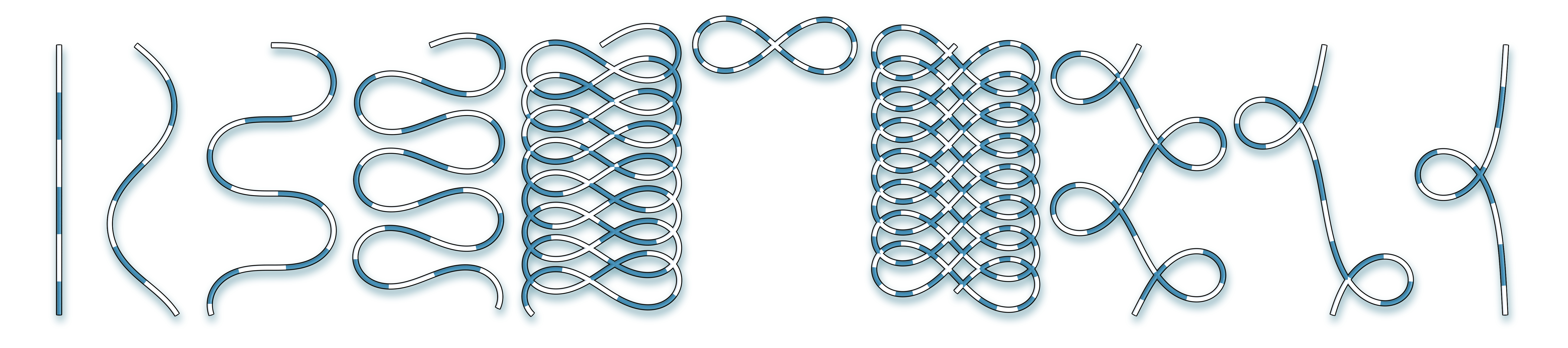
Preliminary numerical experiments suggest that there are a number of interesting closed examples to be discovered. In Fig. 6 we see approximations of planar examples of closed curves which were obtained from integrating Eq. (5.3).
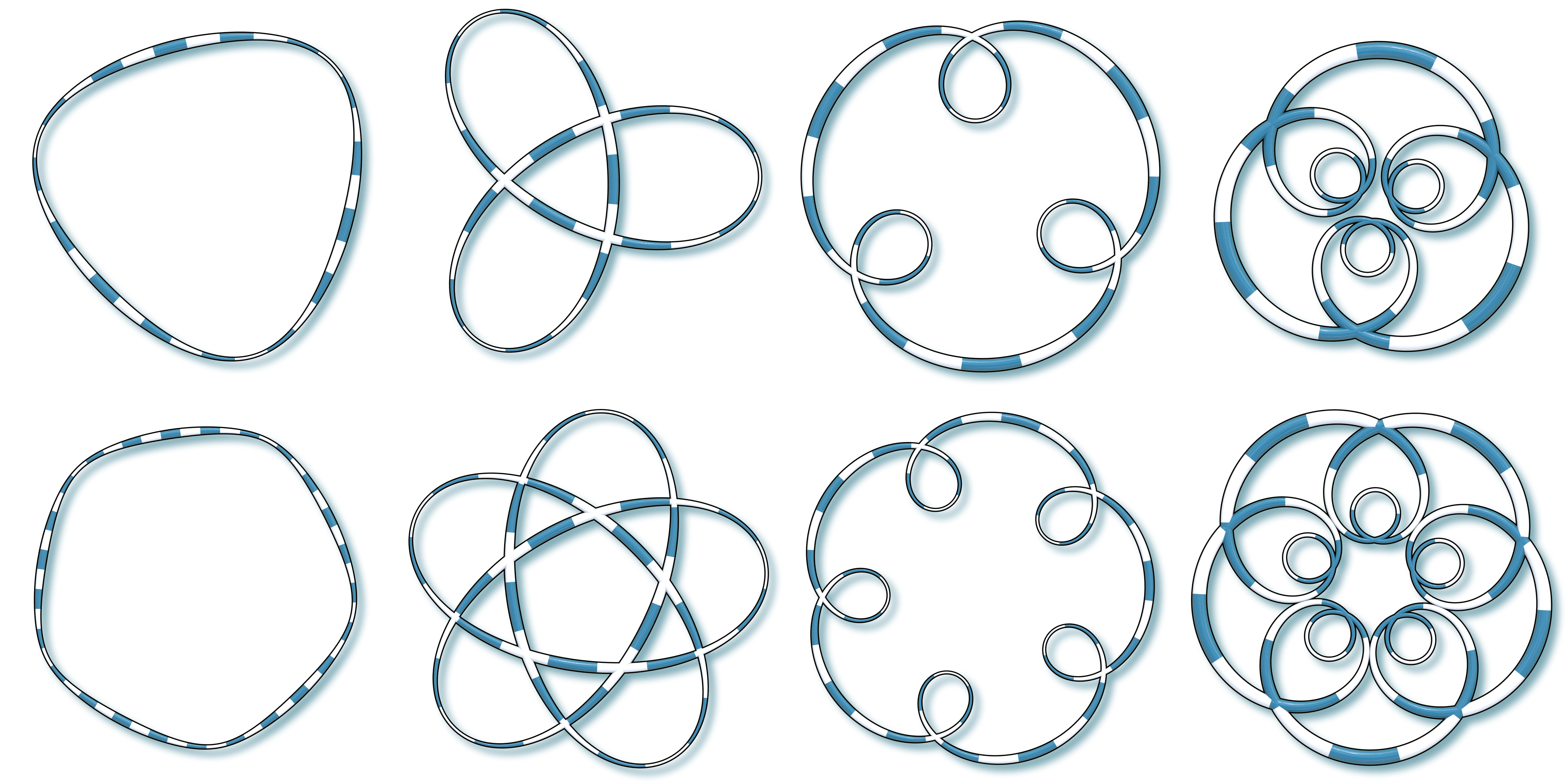
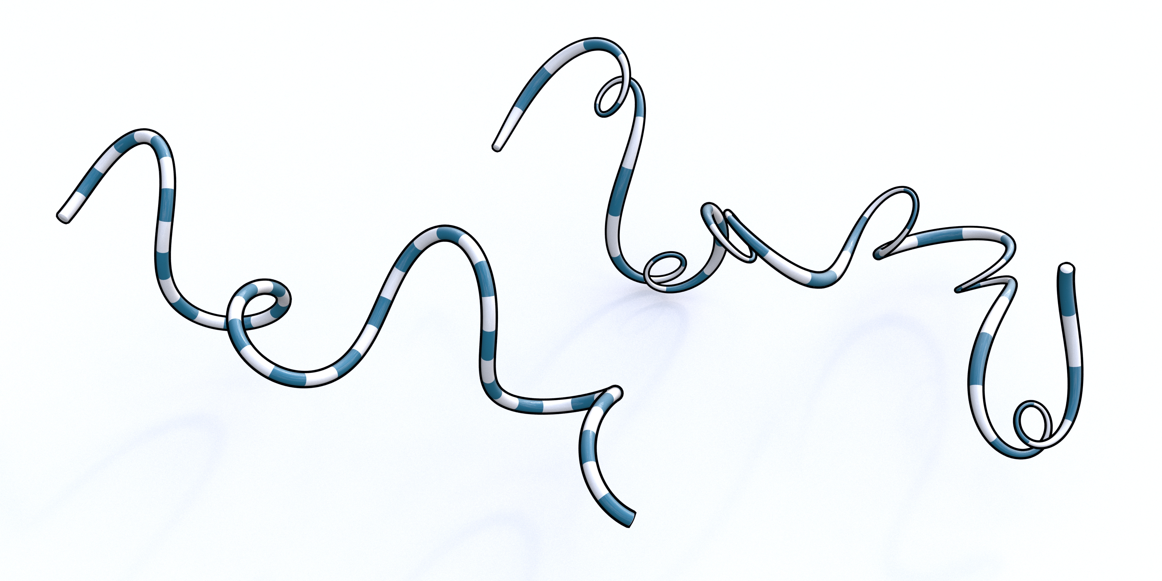
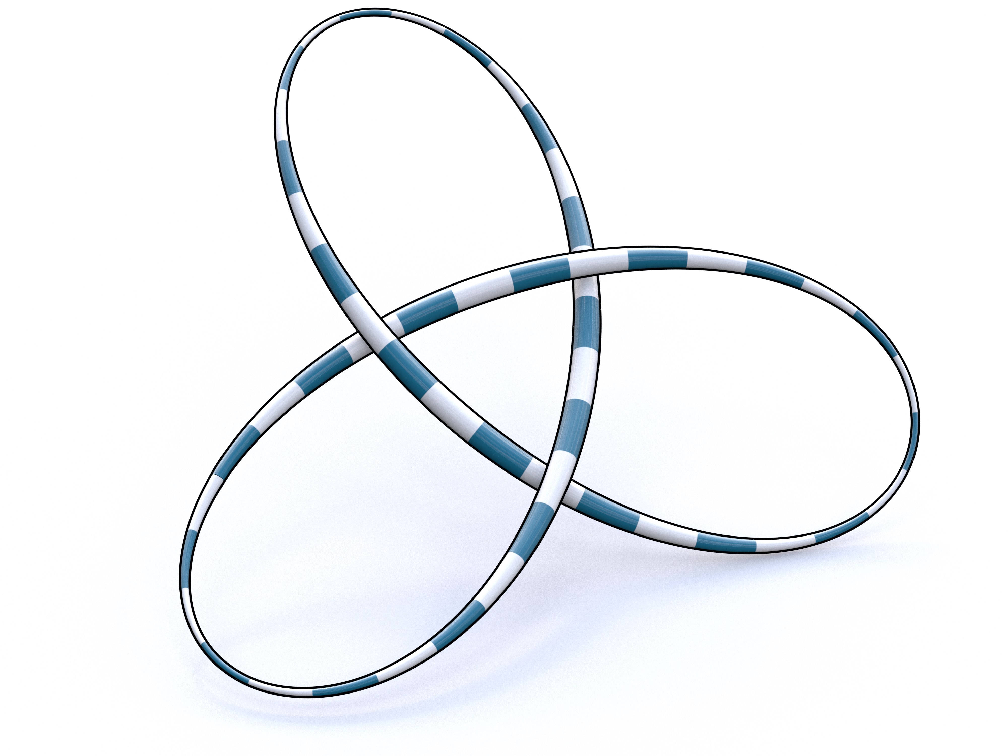
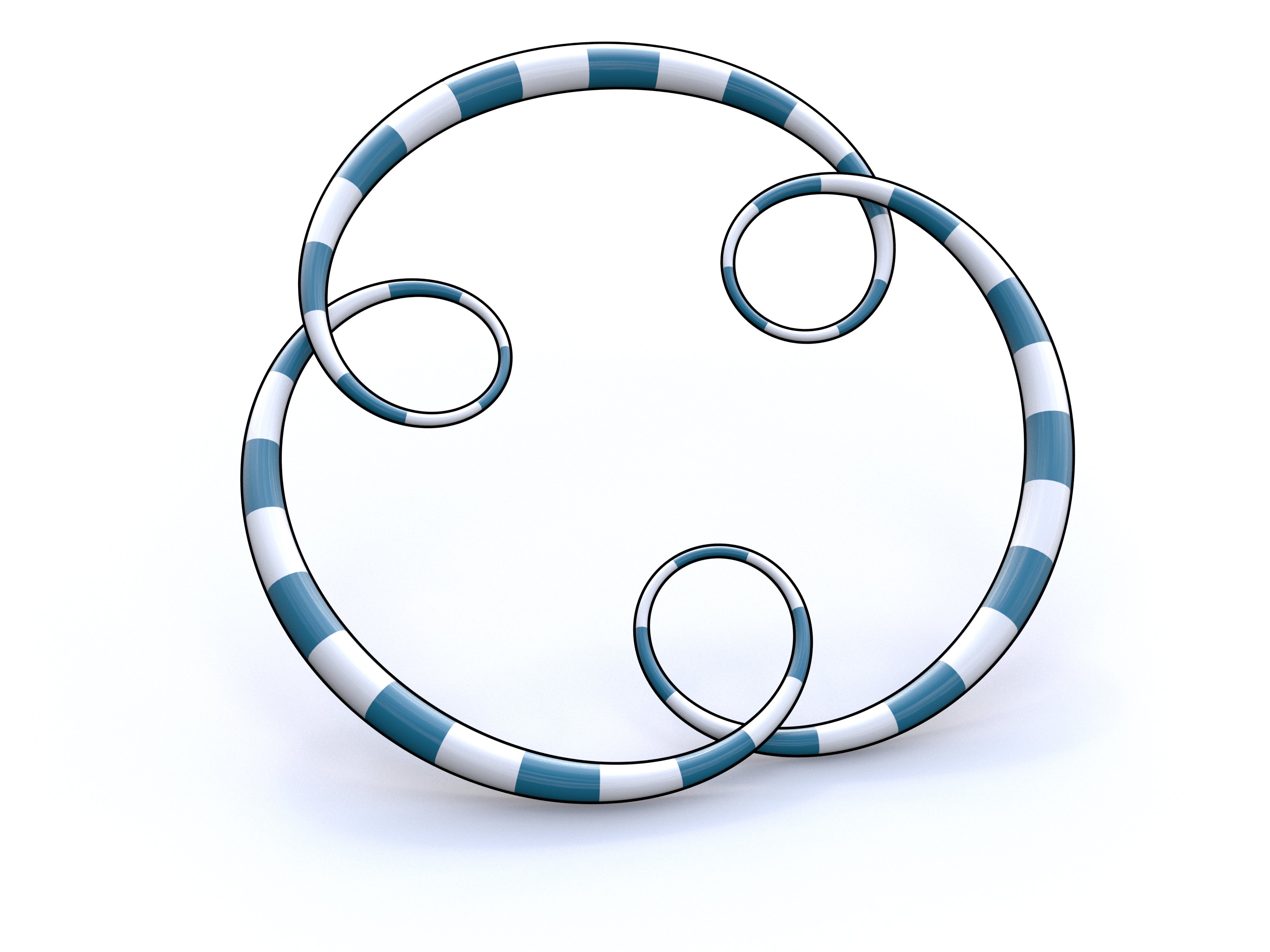
By adding torsion, to each of the planar examples, we expect to find a corresponding -parameter family of three-dimensional examples [15]. Approximations of such non-planar closed elastic curves corresponding to planar examples in Fig. 6 were obtained from integrating condition 5 in Theorem 4.1 and are depicted in Fig. 7.
Clearly, it would be favorable to have computational methods for generating the curves for which the parameters such as length, total torsion and the bending stiffness can be prescribed as an input. However, these computational aspects as well as an explicit analysis of the closing conditions of the curves (see, e.g., [31]) are beyond the scope of this work.
5. Connections with Dynamical Systems
For the case of planar elastic curves with variable bending stiffness Hafner and Bickel found that planar elastic curves with variable bending stiffness are exactly these curves that are non-tangentially intersected in only their inflection points by a straight line.
Theorem 5.1 ([24]).
A planar, unit-speed curve is a torsion-free elastic curve with bending stiffness if and only if
for some . Equivalently, for some , the following equations are satisfied:
| (5.1) | ||||
| (5.2) |
Notably, Theorem 5.1 generalizes a classical result to the case of variable bending stiffness. It is therefore appropriate to look for other results that can be generalized in this context.
5.1. Pendulum Analogy
For the case of constant bending stiffness, arc-length parameterized elastic curves and the pendulum equation share an intricate relationship [45]. A generalization of this relationship has been established in [40] who gave an anisotropic version of the pendulum equation. With Theorem 5.2 we give a corresponding generalization of this relationship for the case of variable bending stiffness.
Theorem 5.2.
Let be an arc-length parameterized curve with bending stiffness . Then is torsion-free elastic if and only if
| (5.3) |
and the pointwise multiplier is given by:
If is constant, is constant.
Proof.
Similar to the proof of Theorem 4.1 we obtain
| (5.4) |
for torsion-free elastic curves, for some . Eq. (5.3) is the component orthogonal to . Taking the inner product of Eq. (5.4) with yields
which is equivalent to
Using results in the second equation. Conversely, let and satisfy Eq. (5.3) for some . Define
and substitute with and with in Eq. (5.3):
which is equivalent to the integrated differential equation for torsion-free elastic curves with Lagrange multiplier .
To see the last part, take the derivative of and use Eq. (5.3):
∎
Theorem 5.2 shows that depends directly on the integrand of bending energy. In addition to that the proof shows that constant results in a constant Lagrange multiplier, the tension of the curve.
Corollary 5.3.
The bending energy of an arc-length parameterized torsion-free elastic curve is given by
5.1.1. The Planar Case
Restricting our attention to the -dimensional case and defining as well as for we find that the first entry of the vector-valued (5.3) becomes
Assuming that this holds if and only if
| (5.5) |
Notably, Eq. (5.5) describes the motion of a damped sinusoidal driven pendulum: consider a system where a pendulum is immersed in a fluid whose density varies with time due to mixing or other dynamic processes. Furthermore, let us assume that the fluid exhibits viscous damping, and the viscosity of the fluid is influenced by its density. As the density of the fluid changes, so does its viscosity. In our specific example, the viscous damping force experienced by the pendulum due to the fluid is proportional to its angular velocity, . The damping coefficient is a function of , which is influenced by the time derivative of the density through its effect on the viscosity of the fluid. Moreover, since a change of viscosity also influences the buoyancy force experienced by the pendulum mass, the gravity term is scaled in Eq. (5.5).
Although this scenario is somewhat contrived and not typical of most damping mechanisms, it demonstrates how variations in density could potentially contribute to the damping effect experienced by a system in certain specialized cases. Notably, this shows that to some extend, the relation to the pendulum equation can conserved even when accounting for variable bending stiffness.
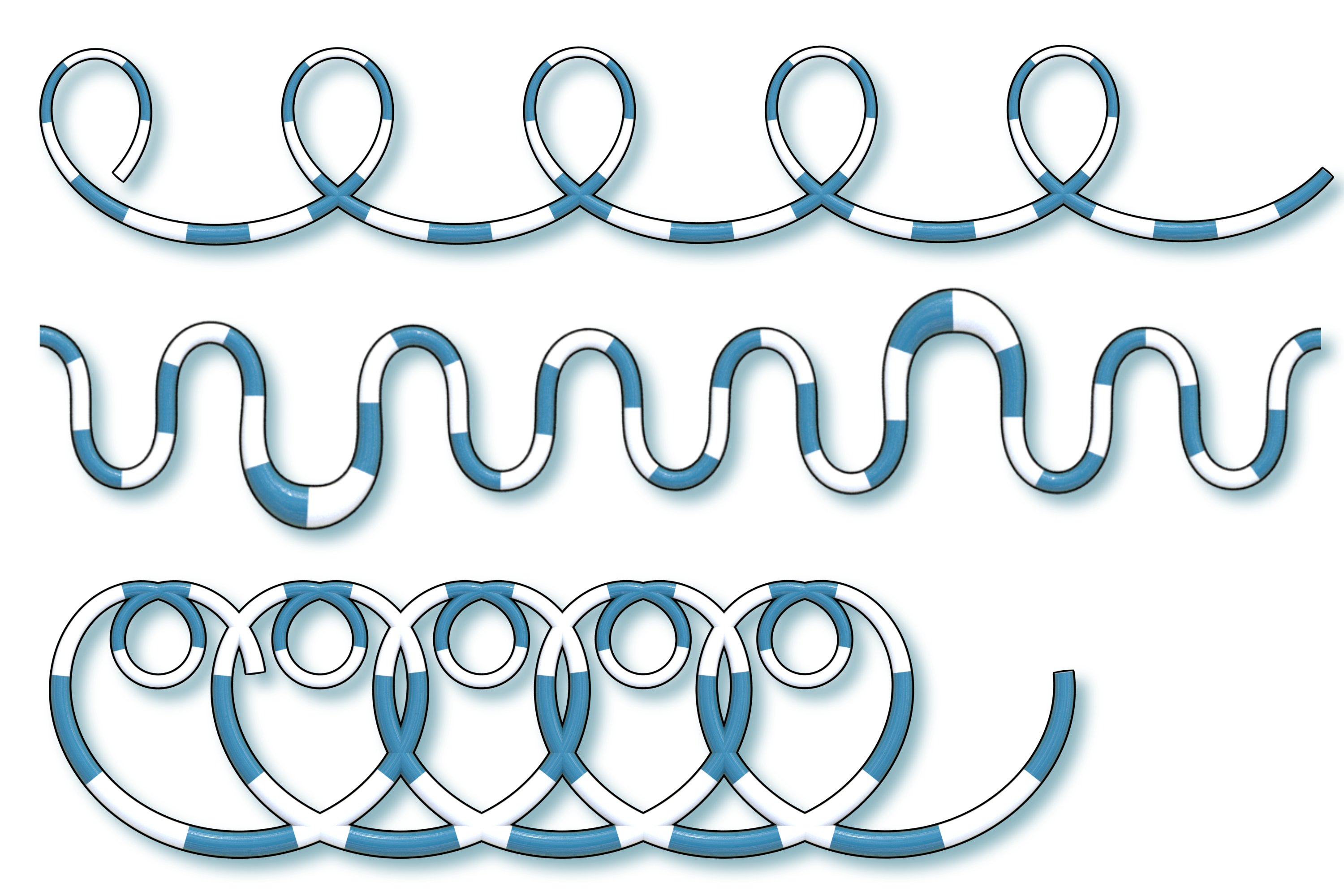
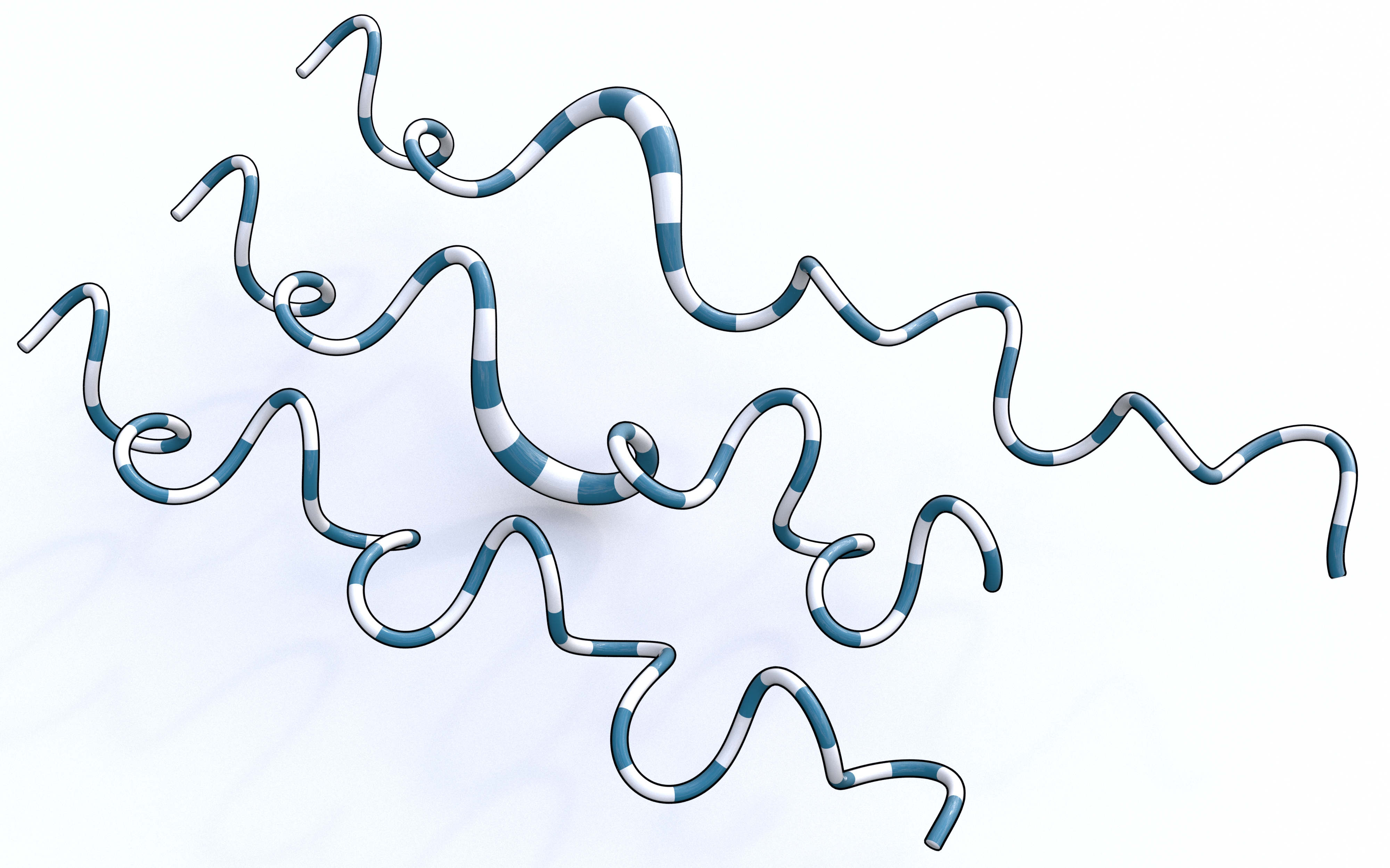
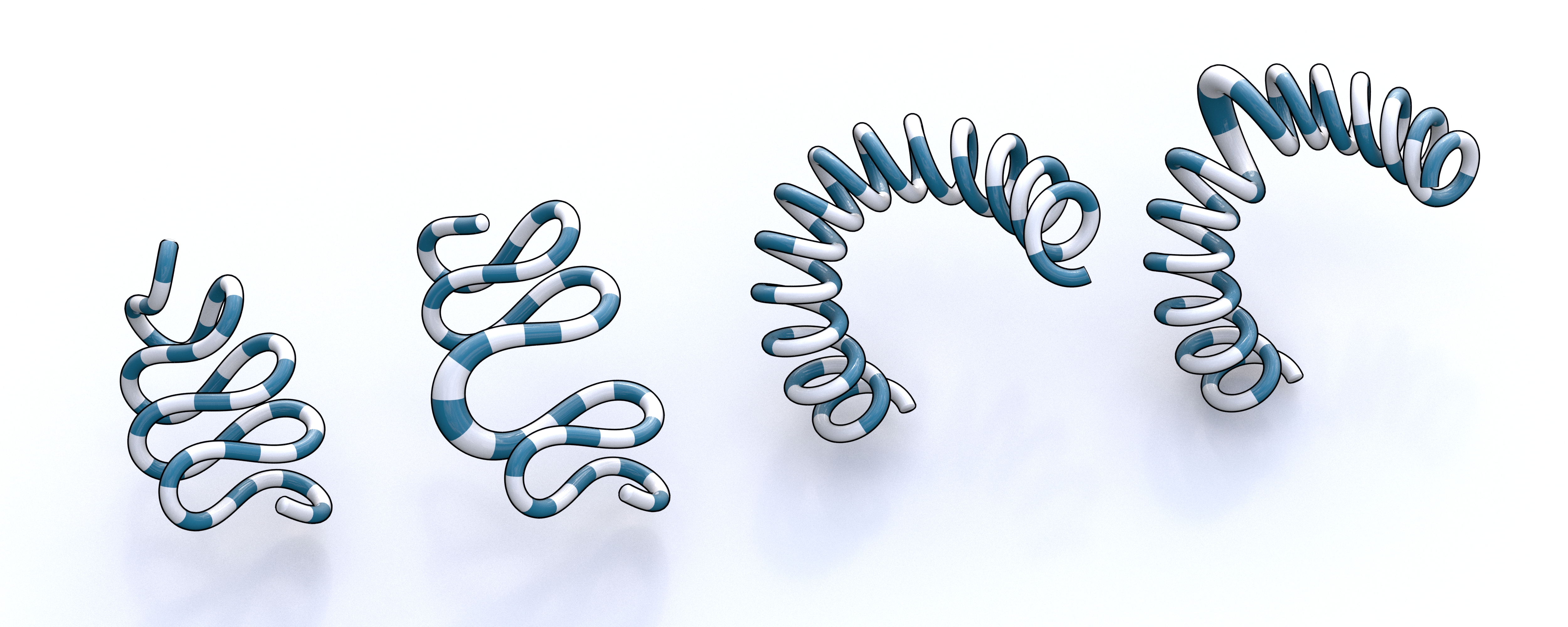
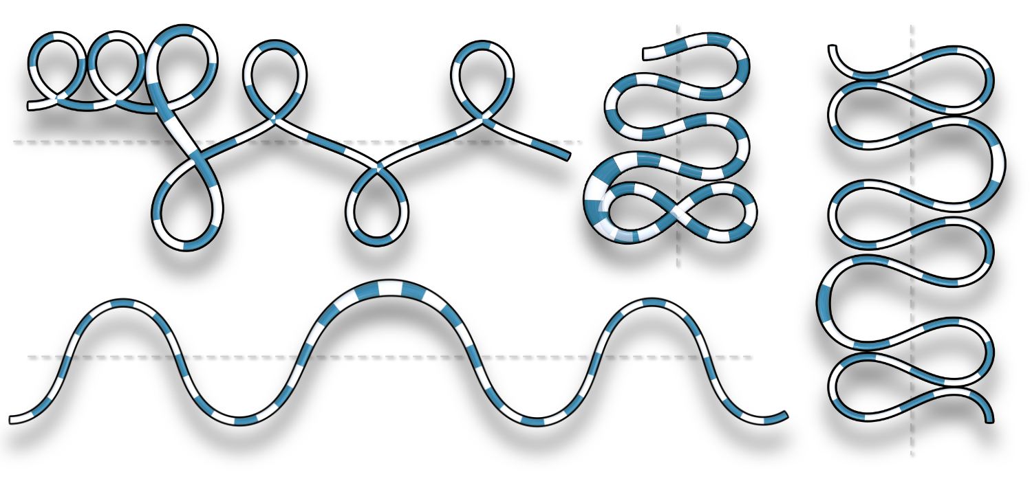
In particular, we find in this analogy an explanation for a phenomenon that we can observe in Fig. 8. If we choose a superposition of a constant function and one (or more) smooth bump functions as the bending stiffness, we see that the usual pendulum equation is fulfilled on sections with constant bending stiffness. Only on sections with non-constant bending stiffness does a dampening effect occur, which can, however, cause a “type change”. This means that the (e.g., viscous) damping or an excitation of the pendulum mass between the phenotypes of the classical planar elastics is caused by different initial conditions.
5.2. Vortex Filament Flow
In this section we will investigate the relations between elastic curves (with variable bending stiffness) and the dynamical behaviour of thin vortex filaments with variable thickness in an incompressible viscous fluid (see, e.g., [39, 13]).
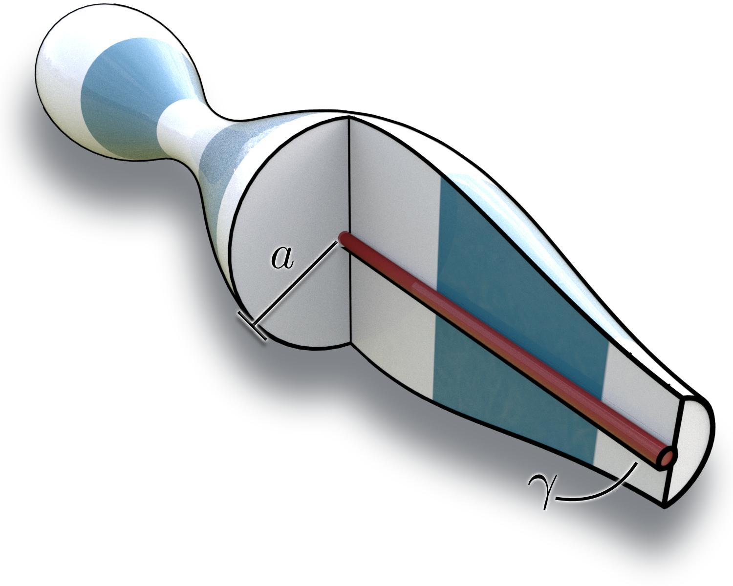
Definition 5.4.
A vortex filament is a map . Together with an additional function a vortex filament is a vortex filament with thickness.
As with rods of variable bending stiffness, we imagine a vortex filament with thickness to be the geometry swept out by a round disc of radius , perpendicular to and centered at . Based on a geometric problem formulation, Padilla et al. [39] gave first-order equations of motion of these filaments with variable thickness in an incompressible viscous fluid. In the absence of gravity [39, Eq. (13)] states that, for the time evolution of a unit strength vortex-filament is (up to a constant) given by
where
is the cut-off Biot–Savart integral for a vortex filament of constant thickness (for which ),
is the localized induction term and the last summand is the tangential velocity333the Lagrangian form of a viscous Burgers’ equation ([39, Eq. (14)]).
5.2.1. Asymptotic Analysis for Thin Vortex Filaments
We note that becomes infinite in the limit , i.e., the vortex filament moves infinitely fast. Therefore, for small filament thickness , the localized induction term becomes the dominating term for the filament evolution.
By a suitable re-scaling of the time, we can control this behaviour (slowing down the “playback speed” of the filament evolution) and reveal some non-trivial relation to elastic curves with variable thickness. To this end we define for some . Then, and with , we get
Now, on the one hand, for a sufficiently large choice of , say , we can achieve
thus preventing the localized induction term to blow up by a suitable re-scaling of time. On the other hand, for large the other two terms become negligible. Therefore, the vortex filament flow for thin vortex filaments of variable thickness is given by
In particular, the re-distribution of filament thickness according to the viscous Burgers’ equation becomes negligible, hence the filament thickness a time-independent function of the arc-length of the filament. With
we arrive at
which, after reparametrization by arc-length, agrees with the left-hand side of Theorem 4.1 4. This leads us to conclude
Theorem 5.5.
Let be a curve with variable bending stiffness . Then is elastic if and only if regarded as a thin vortex filament with variable thickness for , its evolution under vortex filament flow, modulo reparametrization, is given by Euclidean motion.
In particular, we see that for the special case of filaments with constant thickness, the result agrees with the known case (see, e.g., [13]):
Corollary 5.6 ([13, Cor. 2 (v)]).
A curve is elastic if and only if the vortex filament flow evolves, modulo reparametrization, by a Euclidean motion with axis along the monodromy of the initial curve .
Acknowledgements
This work was funded in part by the Deutsche Forschungsgemeinschaft (DFG - German Research Foundation) - Project-ID 195170736 - TRR109 “Discretization in Geometry and Dynamics.” Additional support was provided by SideFX software.
References
- [1] Changyeob Baek and Pedro M. Reis “Rigidity of hemispherical elastic gridshells under point load indentation” In J. Mech. Phys. Solids 124, 2019, pp. 411–426 DOI: 10.1016/j.jmps.2018.11.002
- [2] Craig J. Benham and Steven P. Mielke “DNA Mechanics” In Ann. Rev. Biomed. Eng. 7.1, 2005, pp. 21–53 DOI: 10.1146/annurev.bioeng.6.062403.132016
- [3] M. Bergou, M. Wardetzky, S. Robinson, B. Audoly and E. Grinspun “DiscreteElasticRod” In ACM Trans. Graph. 27.3, 2008 DOI: 10.1145/1360612.1360662
- [4] Felicia Bernatzki and Rugang Ye “Minimal Surfaces with an Elastic Boundary” In Ann. Glob. Anal. 19, 2001 DOI: 10.1023/A:1006734619701
- [5] Florence Bertails, Basile Audoly, Marie-Paule Cani, Bernard Querleux, Frédéric Leroy and Jean-Luc Lévêque “Super-helices for predicting the dynamics of natural hair” In ACM SIGGRAPH 2006 Papers ACM, 2006, pp. 1180–1187 DOI: 10.1145/1179352.1142012
- [6] Florence Bertails-Descoubes, Alexandre Derouet-Jourdan, Victor Romero and Arnaud Lazarus “Inverse design of an isotropic suspended Kirchhoff rod: theoretical and numerical results on the uniqueness of the natural shape” In Proc. R. Soc. Lond. A 474.2212, 2018 DOI: 10.1098/rspa.2017.0837
- [7] Alexander I. Bobenko and Yu.. Suris “A discrete time Lagrange top and discrete elastic curves”, 2000 DOI: 10.1090/trans2/201
- [8] David Brander, Jakob Andreas Bærentzen, Ann-Sofie Fisker and Jens Gravesen “Bézier curves that are close to elastica” In Comp. Aid. Des. 104, 2018 DOI: 10.1016/j.cad.2018.05.003
- [9] Katharina Brazda, Gaspard Jankowiak, Christian Schmeiser and Ulisse Stefanelli “Bifurcation of elastic curves with modulated stiffness”, 2021 DOI: 10.1017/S0956792521000371
- [10] T. Bretl and Z. McCarthy “Quasi-static manipulation of a Kirchhoff elastic rod based on a geometric analysis of equilibrium configuration” In Int. J. Rob. Res. 33, 2014 DOI: 10.1177/0278364912473169
- [11] Marcel Campen and Leif Kobbelt “Dual Strip Weaving: Interactive Design of Quad Layouts using Elastica Strips” In ACM Trans. Graph. 33.6, 2014 DOI: 10.1145/2661229.2661236
- [12] J. Cantarella, R.. Kusner and J.. Sullivan “On the minimum ropelength of knots and links” In Invent. Math. 150 Springer, 2002, pp. 257–286 DOI: 10.1007/s00222-002-0234-y
- [13] Albert Chern, Felix Knöppel, Franz Pedit and Ulrich Pinkall “Commuting Hamiltonian Flows of Curves in Real Space Forms” In Integrable Systems and Algebraic Geometry 1, London Mathematical Society Lecture Note Series Cambridge University Press, 2020, pp. 291–328 DOI: 10.1017/9781108773287.013
- [14] J.. Coolidge “The Unsatisfactory Story of Curvature” In Amer. Math. Month. 59.6, 1952, pp. 375–379 DOI: 10.1080/00029890.1952.11988145
- [15] F Brock Fuller “The writhing number of a space curve” In Proc. Nat. Acad. Sci. 68.4 National Acad Sciences, 1971, pp. 815–819 DOI: 10.1073/pnas.68.4.81
- [16] Patrick B. Furrer, Robert S. Manning and John H. Maddocks “DNA Rings with Mutiple Energy Minima” In Biophys. J. 79 Elsevier Inc., 2000 DOI: 10.1016/S0006-3495(00)76277-1
- [17] L. Giomi and L. Mahadevan “Minimal surfaces bounded by elastic lines” In Proc. R. Soc. Lond. A 468, 2012 DOI: 10.1098/rspa.2011.0627
- [18] Giulio G. Giusteri, Luca Lussardi and Eliot Fried “Solution of the Kirchhoff Plateau Problem” In J. Nonlin. Sc. 27.3 Springer ScienceBusiness Media LLC, 2017, pp. 1043–1063 DOI: 10.1007/s00332-017-9359-4
- [19] Oscar Gonzalez and John H. Maddocks “Global Curvature, Thickness, and the Ideal Shapes of Knots” In Proc. Nat. Acad. Sci. 96.9 National Academy of Sciences, 1999, pp. 4769–4773 DOI: 10.1073/pnas.96.9.4769
- [20] Alain Goriely and Sébastien Neukirch “Mechanics of Climbing and Attachment in Twining Plants” In Phys. R. Lett. 97 American Physical Society, 2006, pp. 184302 DOI: 10.1103/PhysRevLett.97.184302
- [21] Alain Goriely and Michael Tabor “Spontaneous Helix Hand Reversal and Tendril Perversion in Climbing Plants” In Phys. R. Lett. 80 American Physical Society, 1998, pp. 1564–1567 DOI: 10.1103/PhysRevLett.80.1564
- [22] V.G.A Goss “Snap buckling, writhing and loop formation in twisted rods”, 2003
- [23] S. Goyal, N.C. Perkins and C.L. Lee “Nonlinear dynamics and loop formation in Kirchhoff rods with implications to the mechanics of DNA and cables” In J. Comput. Phys. 209.1, 2005 DOI: 10.1016/j.jcp.2005.03.027
- [24] Christian Hafner and Bernd Bickel “The design space of plane elastic curves” In ACM Trans. Graph. 40, 2021, pp. 1–20 DOI: 10.1145/3450626.3459800
- [25] Christian Hafner and Bernd Bickel “The Design Space of Kirchhoff Rods” In ACM Trans. Graph. 40.4, 2023 DOI: 10.1145/3606033
- [26] Hidenori Hasimoto “A soliton on a vortex filament” In J. Fl. Mech. 51.3 Cambridge University Press, 1972, pp. 477–485 DOI: https://doi.org/10.1017/S0022112072002307
- [27] Michael Helmers “Snapping elastic curves as a one-dimensional analogue of two-component lipid bilayers” In Math. Models Methods Appl. Sci. 21.05 World Scientific, 2011, pp. 1027–1042 DOI: 10.1142/S0218202511005234
- [28] Gustav Kirchhoff “Ueber das Gleichgewicht und die Bewegung eines unendlich dünnen elastischen Stabes.” In J. Reine Angew. Math. 1859.56, 1859, pp. 285–313 DOI: 10.1515/crll.1859.56.285
- [29] Petr Kmoch, Ugo Bonanni and Nadia Magnenat-Thalmann “Hair simulation model for real-time environments” In Computer Graphics International Conference, 2009 DOI: 10.1145/1629739.1629740
- [30] Joel Langer and David A Singer “The total squared curvature of closed curves” In J. Diff. Geom. 20.1 Lehigh University, 1984, pp. 1–22 DOI: 10.4310/jdg/1214438990
- [31] Joel C. Langer and David A. Singer “Lagrangian Aspects of the Kirchhoff Elastic Rod” In SIAM Rev. 38, 1996 DOI: 10.1137/S00361445932532
- [32] Joel C. Langer and David A. Singer “Knotted Elastic Curves in ” In J. Lond. Math. Soc. s2-30.3, 1984, pp. 512–520 DOI: 10.1112/jlms/s2-30.3.512
- [33] Raphael Linus Levien “From Spiral to Spline: Optimal Techniques in Interactive Curve Design”, 2009
- [34] J. Lienhard, H. Alpermann, C. Gengnagel and J. Knippers “Active Bending, a Review on Structures where Bending is Used as a Self-Formation Process” In Int. J. Space Struc. 28.3–4, 2013 DOI: 10.1260/0266-3511.28.3-4.187
- [35] Mingchao Liu, Lucie Domino and Dominic Vella “Tapered elasticae as a route for axisymmetric morphing structures” In Soft Mat. 16, 2020, pp. 7739–7750 DOI: 10.1039/D0SM00714E
- [36] H.. Moffatt “The energy spectrum of knots and links” In Nature 347.6291 Nature, 1990, pp. 367–369 DOI: 10.1038/347367a0
- [37] D.E. Moulton, T. Lessinnes and A. Goriely “Morphoelastic rods. Part I: A single growing elastic rod” In J. Mech. Phys. Solids 61.2, 2013, pp. 398–427 DOI: 10.1016/j.jmps.2012.09.017
- [38] Sébastien Neukirch “Extracting DNA Twist Rigidity from Experimental Supercoiling Data” In Phys. R. Lett. 93 American Physical Society, 2004 DOI: 10.1103/PhysRevLett.93.198107
- [39] Marcel Padilla, Albert Chern, Felix Knöppel, Ulrich Pinkall and Peter Schröder “On Bubble Rings and Ink Chandeliers” In ACM Trans. Graph. 38.4 ACM, pp. 129:1–129:14 DOI: 10.1145/3306346.3322962
- [40] Bennett Palmer and Álvaro Pámpano “Anisotropic bending energies of curves” In Ann. Glob. Anal. Geom. 57 Springer, 2020, pp. 257–287 DOI: 10.1007/s10455-019-09698-1
- [41] Julian Panetta, Mina Konaković-Luković, Florin Isvoranu, Etienne Bouleau and Mark Pauly “X-Shells: A new class of deployable beam structures” In ACM Trans. Graph. 38.4, 2019 DOI: 10.1145/3306346.3323040
- [42] Jesus Pérez et al. “Fabrication of Flexible Rod Meshes” In ACM Trans. Graph. 34.4, 2015 DOI: 10.1145/2766998
- [43] Jesús Pérez, Miguel A. Otaduy and Bernhard Thomaszewski “Computational Design and Automated Fabrication of Kirchhoff-Plateau Surfaces” In ACM Trans. Graph. 36.4, 2017 DOI: 10.1145/3072959.3073695
- [44] Stefan Pillwein and Przemyslaw Musialski “Generalized Deployable Elastic Geodesic Grids” In ACM Trans. Graph. 40.6, 2021 DOI: 10.1145/3478513.3480516
- [45] U. Pinkall and O. Gross “Differential Geometry: From Elastic Curves to Willmore Surfaces”, Compact Textbooks in Mathematics Birkhäuser, 2024 DOI: 10.1007/978-3-031-39838-4
- [46] David A. Singer “Lectures on Elastic Curves and Rods” In AIP Conf. Proc. 1002.1, 2008, pp. 3–32 DOI: 10.1063/1.2918095
- [47] Jonas Spillmann and Matthias Harders “Inextensible elastic rods with torsional friction based on Lagrange multipliers” In Comp. An. & Virt. Worlds 21, 2010 DOI: 10.1002/cav.362
- [48] Jonas Spillmann and Matthias Teschner “CoRdE: Cosserat rod elements for the dynamic simulation of one-dimensional elastic objects” In Proc. Symp. Comp. Anim., 2007 DOI: 10.2312/SCA/SCA07/063-072
- [49] Jonas Spillmann and Matthias Teschner “Cosserat nets” In IEEE Trans. Vis. Comp. Graph. 15, 2008 DOI: 10.1109/TVCG.2008.102
- [50] D.M. Stump “The hockling of cables: a problem in shearable and extensible rods” In Int. J. Solid Struc. 37.3, 2000 DOI: 10.1016/S0020-7683(99)00019-0
- [51] Ekkehard-Heinrich Tjaden “Einfache elastische Kurven”, 1991
- [52] Michele Vidulis, Yingying Ren, Julian Panetta, Eitan Grinspun and Mark Pauly “Computational Exploration of Multistable Elastic Knots” In ACM Trans. Graph. 42.4, 2023, pp. 1–15 DOI: 10.1145/3592399
- [53] J. Zehnder, S. Coros and B. Thomaszewski “Designing Structurally-Sound Ornamental Curve Networks” In ACM Trans. Graph. 35.4, 2016 DOI: 10.1145/2897824.2925888
- [54] Eberhard Zeidler “Applied functional analysis: main principles and their applications” Springer, 2012 DOI: 10.1007/978-1-4612-0821-1