Colored Gaussian DAG models

Abstract.

We study submodels of Gaussian DAG models defined by partial homogeneity constraints imposed on the model error variances and structural coefficients. We represent these models with colored DAGs and investigate their properties for use in statistical and causal inference. Local and global Markov properties are provided and shown to characterize the colored DAG model. Additional properties relevant to causal discovery are studied, including the existence and non-existence of faithful distributions and structural identifiability. Extending prior work of Peters and Bühlman and Wu and Drton, we prove structural identifiability under the assumption of homogeneous structural coefficients, as well as for a family of models with partially homogenous structural coefficients. The latter models, termed BPEC-DAGs, capture additional insights as they cluster the direct causes of each node into communities according to their effect on their common target. An analogue of the GES algorithm for learning BPEC-DAGs is given and evaluated on real and synthetic data. Regarding model geometry, we prove that these models are contractible, smooth, algebraic manifolds and compute their dimension. We also provide a proof of a conjecture of Sullivant which generalizes to colored DAG models, colored undirected graphical models and ancestral graph models.

1. Introduction

Directed acyclic graphs (DAGs) and their associated DAG models are fundamental to the field of causal inference; see for instance, the [Drt18, KF09, MDLW18, Pea09, PJS17]. Although defined nonparametrically, a substantial amount of research focuses on DAG models for specified families of parametric distributions, with a popular choice being the Gaussian family. A Gaussian DAG model is a linear structural equation model with independent, normally distributed errors where the structural equations are specified by the edges of the associated DAG. Each edge $i\rightarrow j$ of the DAG is assigned a real-valued parameter $\lambda_{ij}$ serving as its associated structural coefficient. When unconcerned with first moments, we may assume that the error variables associated to each node $i$ in the DAG have mean $0$ and therefore contribute a single additional parameter $\omega_{i}>0$, i.e., its error variance.

When interpreted causally, the edges $i\rightarrow j$ of the DAG are taken to represent direct causal relations with the structural coefficient $\lambda_{ij}$ interpreted as the direct causal effect of the variable $X_{i}$ on $X_{j}$. From the perspective of inference, two natural tasks arise: the first being to identify the direct causal relations from a random sample from the joint distribution contained in the DAG model, and the second to identify the causal effects $\lambda_{ij}$. In the case of Gaussian DAG models, the latter problem has a well-known solution, as the model is known to satisfy global rational identifiability [Drt18]. On the other hand, it is also well-known that different DAGs can represent the same collection of linear SEMs, which implies that the underlying causal DAG may not be identifiable from observational data alone. This is a phenomenon termed Markov equivalence of DAGs, which occurs more generally in the non-parametric setting.

Among the many advantages of DAG models is their admittance of local and global Markov properties, which, in the parametric setting, amount to a family of polynomial constraints that define the model. By way of these constraints, several characterizations of Markov equivalence have been obtained [AMP97, Chi13, VP90a], and the corresponding graphical constraints have been utilized in the development of causal discovery algorithms which are used to estimate the Markov equivalence class of the data-generating DAG from a random sample; see, for example, [Chi02, SWU21, SG91].

A natural consideration for these causal discovery algorithms is to identify the conditions under which they are consistent. The conventional assumption under which we expect such an algorithm to be consistent is known as faithfulness, which assumes that the data-generating distribution satisfies precisely the set of constraints associated to the global Markov property of the causal DAG. An important feature of the Gaussian DAG models is that a generic distribution in the model is faithful to its DAG [SGS00], meaning that standard causal discovery algorithms will consistently estimate its Markov equivalence class (MEC).

However, from the causal perspective, an accurate estimate of the MEC of the causal DAG remains less than ideal, as it often leaves the direction of multiple edges in the graph undetermined; meaning that we cannot recover the direction of causation. Hence, a substantial amount of research has focused on methods for determining the true causal DAG from within its MEC. The gold standard approach, is of course to use available experimental data, which depending on the nodes targeted, may completely or only partially refine the MEC [HB12, YKU18]. While effective, such methods are only applicable in situations where experimental data is available, which is often expensive or even unethical to obtain.

Alternatively, a growing body of research has focused on using additional parametric assumptions on the distribution to achieve structural identifiability; i.e., the identification of the true DAG defining the data-generating SEM. Methods observed to yield structural identifiability include, among others, using linear models with non-Gaussian errors [SHH${}^{+}$06, Shi14], using nonlinear models with additive noise [HJM${}^{+}$08], and in the Gaussian linear SEM setting, imposing homoscedasticity [PB14] or partial homoscedasticity [WD23] constraints.

The methods of [PB14, WD23] obtain structural identifiability for Gaussian DAG models by imposing equality constraints $\omega_{i}=\omega_{j}$ on the error variances in the model. Wu and Drton consider specifically partial homoscedasticity constraints, in which nodes in the DAG are partitioned into classes in which their associated error variances are all equal. To represent these constraints graphically, they color vertices in the DAG the same whenever their error variances are assumed to be equal. This utilizes a special case of the more general representation of a colored DAG, recently introduced in [MRS22], in which nodes are colored the same whenever $\omega_{i}=\omega_{j}$ and edges are colored the same whenever $\lambda_{ij}=\lambda_{k\ell}$. In [PB14], the authors motivated their homoscedasticity assumption as being applicable in situations where the variables are derived from similar domains; analogously one may interpret edge colors as representing similar causal effects.

Our contributions

Based on the recent activity around colored Gaussian DAG models, we establish in this paper some basic properties of these models that will be of general use for their emerging applications. Our aims are three-fold: The first is to establish extensions of the fundamental properties for (uncolored) Gaussian DAG models to the recently introduced colored DAG models of [MRS22]. In Section 3, we derive local and global Markov properties for the colored Gaussian DAG models. In direct analogy to the uncolored Gaussian DAG models, we prove that these Markov properties each provide an alternative definition of the model via a collection of polynomial constraints satisfied by every distribution in the model. We additionally provide some fundamental geometric properties of colored DAG models, deriving the model dimension and proving that each colored DAG model is a smooth submanifold of the positive definite cone (Theorem 4.1). These properties allow for the use of standard techniques from large-sample asymptotic theory when performing likelihood ratio tests [Drt09].

Second, in Section 5, we investigate the existence of faithful distributions in colored DAG models and structural identifiability. In subsection 5.1, we make precise the notion of faithfulness to a colored DAG and show that when a model has only colored edges or colored vertices then a generic distribution in the model will be faithful. In contrast to the uncolored setting, we observe that there exist colored DAG models that do not contain faithful distributions. In Subsection 5.2, we provide structure identifiability results providing edge-colored analogues to the identifiability results of both [PB14] and [WD23]. Namely, we show that structural identifiability is obtained when all structural coefficients $\lambda_{ij}$ are equal, as well as in a special case where edges with equal structural coefficients are assumed target the same node. The latter condition provides us with a family of colored DAG models which can be interpreted as clustering the direct causes of each node in the graph into causal communities based on similar causal effects. In Section 6, we provide an analogoue of the GES causal discovery algorithm [Chi02], which provides estimates of the causal DAG together with additional information on how the causes are clustered into causal communities. The method is evaluated on both real and synthetic data, where our algorithm appears to outperform GES at learning dense causal DAGs, while offering the additional benefits of causal community identification and structurally identifiable DAG estimates.

Our third main contribution is a proof of a conjecture of Sullivant [Sul18] regarding the algebraic structure of uncolored Gaussian DAG models. The conjecture is motivated by an effort to understand exactly how the set of polynomial constraints defining the model via its Markov properties relates to the model’s definition as the image of a rational map. Solutions to such conjectures have potential for applications in the identification of polynomial constraints for rationally parametrized statistical models where the analogue of a global Markov property is not well-understood. We provide a short proof of this conjecture that proves the result in the more general context of Gaussian colored DAG models, colored undirected graphical models [HL08, Lau96], as well as ancestral graph models [RS02]. In Section 7, we end with a brief summary of future directions for futher development of the family of colored Gaussian DAG models as motivated by the results derived in this paper.

2. Preliminaries

This section summarizes basic notation and results for Gaussian DAG models that will be used throughout the paper. For readers familiar with the basic theory of graphical models, this section serves mainly as a reference for notation.

2.1. Graph theory

Given a positive integer $p$, we denote $G=(V,E)$ to be a directed acyclic graph (DAG) on $p$ vertices where $V=[p]$ and $E$ is the set of edges. A topological ordering of the DAG $G$ is a linear ordering $\pi=\pi_{1}\ldots\pi_{p}$ of its vertices such that $i$ precedes $j$ in $\pi$ whenever $i\rightarrow j$ is an edge in $G$. If $i\rightarrow j$ is an edge in $G$, then $i$ is a parent of $j$ and $j$ is a child of $i$ in $G$. A sequence of distinct vertices $(i_{1},\ldots,i_{m})$ such that there exists an edge between $i_{k}$ and $i_{k+1}$ (in any direction) for all $k\in[m-1]$ is called a path in $G$. A path is called directed if the edges are directed as $i_{k}\rightarrow i_{k+1}$ for all $k\in[m-1]$. If there exists a directed path from $i$ to $j$ in $G$, then $i$ is called an ancestor of $j$ and $j$ is called a descendant of $i$. If $j\neq i$ and $j$ is not a descendant of $i$, then $j$ is called a nondescendant of $i$. A vertex $i$ is a source node in $G$ if there is no incoming edge from any other vertex $j$ to $i$ (i.e., edge of the form $j\rightarrow i$) in the edge set. Similarly, $i$ is called a sink node if there is no outgoing edge from $i$ to any other vertex. As all these definitions are specific to a given DAG $G$, we use the notation $pa_{G}(i),ch_{G}(i),an_{G}(i),de_{G}(i)$, and $nd_{G}(i)$ to denote the parents, children, ancestors, descendants and nondescendants of $i$ in $G$. We further use $\overline{de}_{G}(i)=\{i\}\cup de_{G}(i)$ to denote the closure of descendants.

The skeleton of a DAG $G$ is defined as the undirected version of the DAG, i.e., if $i\rightarrow j$ is an edge in $G$, then $i-j$ is an edge in the skeleton of $G$. The edges $i\rightarrow j$ and $j\leftarrow k$ are said to form a v-structure in $G$ if $i$ and $k$ are not adjacent in $G$. An edge $i\rightarrow j$ is said to be covered in $G$ if $pa_{G}(j)=pa_{G}(i)\cup\{i\}$. If a path contains edges of the form $i\rightarrow j$ and $j\leftarrow k$, then $j$ is said to be a collider vertex within that path. A trek in $G$ from a vertex $i$ to a vertex $j$ is a pair $(P_{L},P_{R})$, where $P_{L}$ is a directed path from some vertex $s$ to $i$ and $P_{R}$ is a directed path from the same vertex $s$ to $j$. Here, $s$ is called the top-most vertex of the trek. In other words, a trek can also be considered as a colliderless path. If $A$, $B$, and $C$ are disjoint subsets of $V$, then $C$ d-separates $A$ and $B$ if every path in $G$ connecting a vertex $i\in A$ to a vertex $j\in B$ contains a vertex $k$ that is either a non-collider that belongs to $C$ or a collider that does not belong to $C$ and has no descendants that belong to $C$.

2.2. Gaussian DAG models

A linear structural equation model (SEM) consists of random vectors $X=[X_{1},\ldots,X_{p}]^{T}$ which satisfy the relation

$$X=\Lambda^{T}X+\varepsilon$$

where $\varepsilon=[\varepsilon_{1},\ldots,\varepsilon_{p}]^{T}$ with $\varepsilon_{1},\ldots,\varepsilon_{p}$ mutually independent and $\Lambda=(\lambda_{ij})$ is a $p\times p$ real matrix. The nonzero entries in the matrix $\Lambda$ determine the dependence relations (sometimes called the causal structure) amongst the variables in the system. In this paper, we assume that this causal structure is representable by a directed acyclic graph (DAG); that is, we assume the matrix $\Lambda$ is strictly upper triangular, in which case we can represent the causal structure of the model via a DAG with edge set $i\rightarrow j$ whenever $\lambda_{ij}\neq 0$.

We will assume throughout that the errors $\varepsilon_{1},\ldots,\varepsilon_{p}$ are normally distributed with mean $0$ and variance $\omega_{i}>0$ for $i=1,\ldots,p$. Under these assumptions $\varepsilon\sim\textrm{N}(0,\Omega)$ where $\Omega=\operatorname{diag}(\omega_{1},\ldots,\omega_{p})$, and $X\sim\textrm{N}(0,\Sigma)$ where

$$\Sigma=(1-\Lambda)^{-T}\Omega(1-\Lambda)^{-1}.$$

Let $G=(V,E)$ be a directed acyclic graph (DAG), where $V=[p]:=\{1,\ldots,p\}$. For convenience, we will often represent the parameter vector $\omega=(\omega_{1},\ldots,\omega_{p})\in\mathbb{R}_{>0}^{p}$ with the diagonal matrix $\Omega=\operatorname{diag}(\omega)$. We obtain (the covariance matrix of) a random vector in the linear structural equation model associated to $G$ for any choice of $\Omega\in\mathbb{R}_{>0}^{p}$ and $\Lambda$ in

$$\mathbb{R}^{E}=\{\Lambda=(\lambda_{ij})\in\mathbb{R}^{V\times V}:\lambda_{ij}=0\textrm{ whenever }i\rightarrow j\notin E\}$$

via the parameterization map

$$\begin{split}\phi_{G}:{}&\mathbb{R}_{>0}^{V}\times\mathbb{R}^{E}\longrightarrow\RM{PD}^{p},\\ &(\Omega,\Lambda)\longmapsto(1-\Lambda)^{-T}\Omega(1-\Lambda)^{-1}.\end{split}$$

Here, $\RM{PD}^{p}$ denotes the cone of all $p\times p$ positive definite matrices. The Gaussian DAG model denoted $\CC M(G)$ is defined to be the collection of multivariate normal distributions with covariance matrix lying in the image of the map $\phi_{G}$. Since we assume all errors have mean $0$, each covariance matrix corresponds to a unique distribution in the model, so we identify the set of distributions $\CC M(G)$ with the set of covariance matrices $\operatorname{im}(\phi_{G})$; that is, $\CC M(G)=\operatorname{im}(\phi_{G})$.

Gaussian DAG models are well-understood, and known to admit several properties that are useful for inference. For instance, the dimension of the model $\CC M(G)$ for $G=(V,E)$ is known to be $|V|+|E|$, and $\CC M(G)$ is a smooth submanifold of the positive definite cone. The latter property implies that standard asymptotic theory for hypothesis testing can be used when performing statistical inference with these models [Drt09].

Gaussian DAG models enjoy several properties relevant to the field of causality. For instance, $\CC M(G)$ can also be characterized as the set of distributions satisfying a collection of conditional independence relations specified by a so-called Markov property with respect to $G=([p],E)$. We say that a distribution $[X_{1},\ldots,X_{p}]^{T}\sim\textrm{N}(0,\Sigma)$ satisfies the

1. local Markov property with respect to $G$ if $X_{i}\mathchoice{\mathrel{\hbox to0.0pt{$\displaystyle\perp$\hss}\mkern 2.0mu{\displaystyle\perp}}}{\mathrel{\hbox to0.0pt{$\textstyle\perp$\hss}\mkern 2.0mu{\textstyle\perp}}}{\mathrel{\hbox to0.0pt{$\scriptstyle\perp$\hss}\mkern 2.0mu{\scriptstyle\perp}}}{\mathrel{\hbox to0.0pt{$\scriptscriptstyle\perp$\hss}\mkern 2.0mu{\scriptscriptstyle\perp}}}X_{\RM{nd}_{G}(i)\setminus\RM{pa}_{G}(i)}\mid X_{\RM{pa}_{G}(i)}$ for all $i\in V$;

2. global Markov property with respect to $G$ if $X_{A}\mathchoice{\mathrel{\hbox to0.0pt{$\displaystyle\perp$\hss}\mkern 2.0mu{\displaystyle\perp}}}{\mathrel{\hbox to0.0pt{$\textstyle\perp$\hss}\mkern 2.0mu{\textstyle\perp}}}{\mathrel{\hbox to0.0pt{$\scriptstyle\perp$\hss}\mkern 2.0mu{\scriptstyle\perp}}}{\mathrel{\hbox to0.0pt{$\scriptscriptstyle\perp$\hss}\mkern 2.0mu{\scriptscriptstyle\perp}}}X_{B}\mid X_{C}$ whenever $A$ and $B$ are d-separated given $C$ in $G$;

3. ordered pairwise Markov property with respect to $G$ if $X_{i}\mathchoice{\mathrel{\hbox to0.0pt{$\displaystyle\perp$\hss}\mkern 2.0mu{\displaystyle\perp}}}{\mathrel{\hbox to0.0pt{$\textstyle\perp$\hss}\mkern 2.0mu{\textstyle\perp}}}{\mathrel{\hbox to0.0pt{$\scriptstyle\perp$\hss}\mkern 2.0mu{\scriptstyle\perp}}}{\mathrel{\hbox to0.0pt{$\scriptscriptstyle\perp$\hss}\mkern 2.0mu{\scriptscriptstyle\perp}}}X_{j}\mid X_{1,\ldots,j-1}$ for all $i<j$ where $i\rightarrow j\notin E$.

A fundamental result in the theory of graphical models states that a distribution lies in $\CC M(G)$ if and only if it satisfies any one of the above Markov properties [Lau96].

Theorem 2.1.

Let $G=([p],E)$ be a DAG and $\Sigma$ a $p\times p$ positive definite matrix. The following are equivalent:

1. $\Sigma\in\CC M(G)$,

2. $\Sigma$ satisfies the local Markov property with respect to $G$,

3. $\Sigma$ satisfies the global Markov property with respect to $G$, and

4. $\Sigma$ satisfies the ordered pairwise Markov property with respect to $G$.

Theorem 2.1 in fact does not require Gaussianity; e.g., it holds in the general (nonparametric) setting. The global Markov property is referred to as such since it describes all conditional independence relations that a distribution is required to satisfy if it belongs to the model $\CC M(G)$. Namely, it is complete, meaning that any conditional independence relation $X_{A}\mathchoice{\mathrel{\hbox to0.0pt{$\displaystyle\perp$\hss}\mkern 2.0mu{\displaystyle\perp}}}{\mathrel{\hbox to0.0pt{$\textstyle\perp$\hss}\mkern 2.0mu{\textstyle\perp}}}{\mathrel{\hbox to0.0pt{$\scriptstyle\perp$\hss}\mkern 2.0mu{\scriptstyle\perp}}}{\mathrel{\hbox to0.0pt{$\scriptscriptstyle\perp$\hss}\mkern 2.0mu{\scriptscriptstyle\perp}}}X_{B}\mid X_{C}$ satisfied by all $\Sigma\in\CC M(G)$ is represented by a d-separation relation in $G$; i.e., $A$ and $B$ are d-separated given $C$ in $G$. The fact that the global Markov property is complete for Gaussian DAG models can be seen from the existence of distributions in the model $\CC M(G)$ that are faithful to $G$. Namely, a distribution $\Sigma\in\CC M(G)$ is said to be faithful to $G$ if $A$ and $B$ are d-separated given $C$ in $G$ whenever $X_{A}\mathchoice{\mathrel{\hbox to0.0pt{$\displaystyle\perp$\hss}\mkern 2.0mu{\displaystyle\perp}}}{\mathrel{\hbox to0.0pt{$\textstyle\perp$\hss}\mkern 2.0mu{\textstyle\perp}}}{\mathrel{\hbox to0.0pt{$\scriptstyle\perp$\hss}\mkern 2.0mu{\scriptstyle\perp}}}{\mathrel{\hbox to0.0pt{$\scriptscriptstyle\perp$\hss}\mkern 2.0mu{\scriptscriptstyle\perp}}}X_{B}\mid X_{C}$ .

The completeness of the global Markov property allows us to recover a characterization of the DAGs $G$ and $H$ that satisfy $\CC M(G)=\CC M(H)$ via purely graph-theoretic means. We say that $G$ and $H$ are Markov- (or model-) equivalent if $\CC M(G)=\CC M(H)$, and we call the set of all DAGs Markov equivalent to $G$ its Markov equivalence class (MEC).

Theorem 2.2 ([VP90a]).

$G$ and $H$ are Markov equivalent if and only if they have the same skeleton and v-structures.

The Markov properties and characterizations of Markov equivalence play a fundamental role in the problem of causal discovery, where one aims to learn the DAG structure $G$ from data.

By the trek rule [Sul18, Proposition 14.2.13], a matrix $\Sigma=(\sigma_{ij})$ satisfies $\Sigma=\phi_{G}(\omega,\Lambda)$ for some $(\omega,\Lambda)\in\mathbb{R}_{>0}^{V}\times\mathbb{R}^{E}$ (i.e., $\Sigma$ belongs to the model $\CC M(G)$) if and only if

(T) $$\sigma_{ij}=\sum_{\begin{subarray}{c}\text{$\tau$ : trek}\\ \text{from $i$ to $j$}\end{subarray}}\omega_{\RM{top}(\tau)}\lambda^{\tau},$$

for all $i,j\in[p]$, where $\omega_{\RM{top}(\tau)}\lambda^{\tau}$ is the trek monomial of $\tau$: namely, if $\tau$ consists of two directed paths $k=i_{n}\to i_{n-1}\to\dots\to i_{0}=i$ and $k=j_{m}\to j_{m-1}\to\dots\to j_{0}=j$, then $\RM{top}(\tau)=k$ and $\lambda^{\tau}=\prod_{\ell=1}^{n}\lambda_{i_{\ell-1}i_{\ell}}\cdot\prod_{\ell=1}^{m}\lambda_{j_{\ell-1}j_{\ell}}$.

The DAG model $\CC M(G)$ also admits parameter identifiability results that are useful in causal inference. It is well-known that the parameters $(\Lambda,\Omega)$ for which $\Sigma=\phi_{G}(\Lambda,\Omega)\in\CC M(G)$ are rationally identifiable, meaning that there are rational functions of the $\sigma_{ij}$ coordinates yielding the $\omega_{i}$ and $\lambda_{ij}$ parameter values defining $\Sigma$. These rational functions are most easily expressed using minors of the covariance matrix $\Sigma$. Given a matrix $\Sigma=[\sigma_{ij}]\in\mathbb{R}^{p\times p}$ and sets $A,B\subseteq[p]$, we let $\Sigma_{A,B}=[\sigma_{ij}]_{i\in A,j\in B}$ denote the submatrix of $\Sigma$ with rows indexed by $A$ and columns indexed by $B$. When $|A|=|B|=m$, we let $|\Sigma_{A,B}|$ denote the determinant of $\Sigma_{A,B}$. The determinant $|\Sigma_{A,B}|$ is a polynomial in the variables $\sigma_{ij}$ that we call an $m$-minor of $\Sigma$. Using this notation, we then have the following formulas for identifying the parameters $(\Lambda,\Omega)$ for which $\Sigma=\phi_{G}(\Lambda,\Omega)$:

($$\omega \omega_{i} =\frac{|\Sigma_{\RM{pa}(i)\cup i}|}{|\Sigma_{\RM{pa}(i)}|},$$)

($$\lambda \Lambda_{\RM{pa}(j),j} =\Sigma_{\RM{pa}(j)}^{-1}\Sigma_{\RM{pa}(j),j}.$$)

The value $\lambda_{ij}$ is sometimes called the causal effect of $i$ on $j$, as it encodes the direct influence of $X_{i}$ on $X_{j}$.

Finally, the interpretation of $\CC M(G)$ as the collection of distributions that satisfy a family of conditional independence relations (as specified by a Markov property above) means that the model can be thought of as the set of all positive definite matrices $\Sigma$ that satisfy a family of polynomial constraints. Namely, $X_{A}\mathchoice{\mathrel{\hbox to0.0pt{$\displaystyle\perp$\hss}\mkern 2.0mu{\displaystyle\perp}}}{\mathrel{\hbox to0.0pt{$\textstyle\perp$\hss}\mkern 2.0mu{\textstyle\perp}}}{\mathrel{\hbox to0.0pt{$\scriptstyle\perp$\hss}\mkern 2.0mu{\scriptstyle\perp}}}{\mathrel{\hbox to0.0pt{$\scriptscriptstyle\perp$\hss}\mkern 2.0mu{\scriptscriptstyle\perp}}}X_{B}\mid X_{C}$ holds if and only if $\Sigma_{A\cup C,B\cup C}$ has rank $|C|$. If $A=\Set{i}$ and $B=\Set{j}$, then this is equivalent to the vanishing of the determinant $|\Sigma_{iC,jC}|$ which we denote by $|\Sigma_{ij|C}|$ in analogy to the conditional independence statement $X_{i}\mathchoice{\mathrel{\hbox to0.0pt{$\displaystyle\perp$\hss}\mkern 2.0mu{\displaystyle\perp}}}{\mathrel{\hbox to0.0pt{$\textstyle\perp$\hss}\mkern 2.0mu{\textstyle\perp}}}{\mathrel{\hbox to0.0pt{$\scriptstyle\perp$\hss}\mkern 2.0mu{\scriptstyle\perp}}}{\mathrel{\hbox to0.0pt{$\scriptscriptstyle\perp$\hss}\mkern 2.0mu{\scriptscriptstyle\perp}}}X_{j}\mid X_{C}$ to which it corresponds. The consequence for DAG models is formalized in the following lemma.

Lemma 2.3.

The Gaussian DAG model $\CC M(G)$ is the collection of all positive definite matrices $\Sigma\in\RM{PD}^{p}$ on which all the polynomials in

$$J_{G}=\ideal{\,\mbox{$(|C|+1)$-minors of }\Sigma_{A\cup C,B\cup C}|\mbox{ $A$ and $B$ are d-separated given $C$ in $G$}\,}.$$

evaluate to zero.

The collection of polynomials $J_{G}$ is sometimes called the (global) conditional independence ideal of the model $\CC M(G)$ [Sul08].

3. Markov properties for colored Gaussian DAG models

A colored DAG is a triple $(V,E,c)$ consisting of a directed acyclic graph $G=(V,E)$ together with a coloring map $c:V\sqcup E\to C$, where $C$ is a finite set and $c(V)\cap c(E)=\emptyset$. We will often denote the colored DAG $(V,E,c)$ simply by $(G,c)$ since $G=(V,E)$. The image of a vertex or edge under this map is referred to as its color. The coloring induces a partition on vertices and edges into color classes. We denote the number of vertex and edge color classes by $\RM{vc}$ and $\RM{ec}$, respectively.

For $\Sigma$ in the DAG model $\CC M(G)$, with corresponding structural equations

$$\begin{split}X_{i}=\sum_{k\in\RM{pa}_{G}(i)}\lambda_{ki}X_{k}+N_{i}\end{split}$$

where $N_{i}\sim\textrm{N}(0,\omega_{i})$, we say that $\Sigma$ is Markov to the colored DAG $(G,c)$ if $\omega_{i}=\omega_{k}$ whenever $c(i)=c(k)$ and $\lambda_{ij}=\lambda_{k\ell}$ whenever $c(ij)=c(k\ell)$.

Definition 3.1.

The colored Gaussian DAG model $\CC M(G,c)$ for the colored DAG $(G,c)$ is the set of all $\Sigma\in\RM{PD}^{p}$ that are Markov to $(G,c)$. That is,

$$\CC M(G,c)=\{\phi_{G,c}(\Omega,\Lambda)\in\RM{PD}^{p}:(\Omega,\Lambda)\in A(G,c)\},$$

where

$$\begin{split}A(G,c)=\{(\operatorname{diag}(\omega_{1},\ldots,\omega_{d}),\Lambda)\in\mathbb{R}_{>0}^{p}\times\mathbb{R}^{p\times p}:{}&\lambda_{ij}=\lambda_{c(ij)}\,\,\forall i\in V,\\ &\omega_{i}=\omega_{c(i)}\,\,\forall ij\in E,\\ &\lambda_{ij}=0\,\,\forall ij\notin E,\\ &\mbox{and }\lambda_{c(ij)}\in\mathbb{R},\omega_{c(i)}\in\mathbb{R}_{>0}\}\end{split}$$

is the colored parameter space and

$$\begin{split}\phi_{G,c}:{}&A(G,c)\longrightarrow\RM{PD}^{p};\\ &(\Omega,\Lambda)\longmapsto(1-\Lambda)^{-T}\Omega(1-\Lambda)^{-1}.\end{split}$$

The colored Gaussian DAG model $\CC M(G,c)$ is therefore the image of the parametrization $\phi_{G,c}$ arising from $\phi_{G}$ (see Subsection 2.2) by replacing all occurrences of parameters in the same color class with a single parameter corresponding to the color class.

We introduce some further terminology that will be used in the paper. Let $(G,c)$ be a colored DAG and $\mathbf{c}$ a color class for $(G,c)$. The color class $\mathbf{c}$ is either a set of nodes or a set of edges of $G$. If $i$ indexes the smallest vertex or $ij$ indexes the smallest edge in $\mathbf{c}$ with respect to the lexicographic ordering from the right on the elements of $\mathbf{c}$, then $\sigma_{ii}$ and $\sigma_{ij}$, respectively, are called the base variables for $\mathbf{c}$, and correspondingly $\omega_{i}$ and $\lambda_{ij}$ are the base parameters.

The uncolored model $\CC M(G)$ is obtained as a special case of the colored model by choosing $C=V\sqcup E$ and $c$ to be the identity map, i.e., each vertex and edge has its own, unique color. In this case, we say that the DAG is uncolored. Analogously, we say that $(G,c)$ is vertex-colored if $c|_{E}$ is the identity and edge-colored if $c|_{V}$ is the identity. Note that $\CC M(G,c)\subseteq\CC M(G)$ for all colorings $c$ of $G$; that is, all colored DAG models are submodels of the corresponding uncolored DAG model.

The classic (uncolored) Gaussian DAG model $\CC M(G)$ may be defined by the parameterization given in Section 2 or, alternatively, as the set of distributions satisfying a collection of conditional independence relations specified by any one of the Markov properies presented in Subsection 2.2. As noted in Section 3, a colored DAG model $\CC M(G,c)$ is a subset of the uncolored DAG model $\CC M(G)$ specified by homogeneity constraints corresponding to the coloring of the vertices and edges of $G$. In this section, we establish a local and a global Markov property for these models. To do so, we begin by characterizing the rational functions of the covariance parameters $\sigma_{ij}$ that may be used to identify the error variances $\omega_{i}$ and structural coefficients $\lambda_{ij}$.

3.1. Parameter identification

Let $G=(V,E)$ be a DAG and let $\Sigma\in\CC M(G)$. Then there exist $(\omega,\Lambda)\in\mathbb{R}_{+}^{V}\times\mathbb{R}^{E}$ such that $\phi_{G}(\omega,\Lambda)=\Sigma$. Since $G$ is acyclic, the parametrization map is injective or, in other words, the parameters $\omega$ and $\Lambda$ are globally identifiable [Sul18, Theorem 16.2.1], [DRW20, Section 3]. Moreover, the parameter recovery map consists of rational functions in the covariance matrix $\Sigma$ whose denominators are specific principal minors and therefore nonzero on $\RM{PD}^{p}$. In the next lemma, we collect explicit formulas for each individual parameter.

Lemma 3.2.

Let $G$ be a DAG and $\phi_{G}$ its trek rule parametrization. For $\Sigma=\phi_{G}(\omega,\Lambda)\in\CC M_{G}$, the $\omega$ and $\Lambda$ parameters are recovered via

($$\omega \omega_{i} =\RM{Var}(X_{i}\mid X_{\RM{pa}(i)})=\frac{|\Sigma_{\RM{pa}(i)\cup i}|}{|\Sigma_{\RM{pa}(i)}|},$$)

($$\lambda \lambda_{ij} =\frac{\RM{Cov}(X_{i},X_{j}\mid X_{\RM{pa}(j)\setminus i})}{\RM{Var}(X_{i}\mid X_{\RM{pa}(j)\setminus i})}=\frac{|\Sigma_{ij|\RM{pa}(j)\setminus i}|}{|\Sigma_{\RM{pa}(j)}|}.$$)

These formulas are known: see [WD23, Theorem 3.1] for ($\omega$) and [SRM${}^{+}$98, Section 4.4] for ($\lambda$) in the more general context of path diagrams. Since a homogeneity constraint amounts to setting $\omega_{i}=\omega_{j}$ or $\lambda_{ij}=\lambda_{k\ell}$, the above rational functions provide constraints that capture when two nodes, or respectively two edges, have the same color; for instance, the function

$$f(\Sigma)=\frac{|\Sigma_{\RM{pa}(i)\cup i}|}{|\Sigma_{\RM{pa}(i)}|}-\frac{|\Sigma_{\RM{pa}(j)\cup j}|}{|\Sigma_{\RM{pa}(j)}|}$$

will evaluate to $0$ on all $\Sigma\in\CC M(G,c)$ where $c(i)=c(j)$ since this equality of colors corresponds to the equality of parameters $\omega_{i}=\omega_{j}$. To formulate a global Markov property for colored DAG models, we would like a description of all such constraints on the model that arise from the chosen coloring. To do so, we characterize the ways in which we may identify the parameter values $\omega_{i}$ and $\lambda_{ij}$ using rational functions of the same form as ($\omega$) and ($\lambda$).

Definition 3.3.

Consider the two rational functions of covariance matrices $\Sigma$:

$$\omega_{i|A}(\Sigma)\defas\frac{|\Sigma_{iA}|}{|\Sigma_{A}|}\quad\text{and}\quad\lambda_{ij|A}(\Sigma)\defas\frac{|\Sigma_{ij|A\setminus i}|}{|\Sigma_{A}|}.$$

Fix a DAG $G=(V,E)$. A set $A\subseteq V$ is identifying for the vertex $i\in V$ if $\omega_{i|A}(\phi_{G}(\Omega,\Lambda))=\omega_{i}$. It is identifying for the edge $ij\in E$ if $\lambda_{ij|A}(\phi_{G}(\Omega,\Lambda))=\lambda_{ij}$. Let $\CC A_{G}(i)$ and $\CC A_{G}(ij)$ denote the sets of $i$- respectively $ij$-identifying sets.

The vertex-identifying sets were completely characterized in recent work of Drton and Wu [WD23, Theorem 3.3]. A sufficient condition for a set to be edge-identifying is proven in Spirtes et al. [SRM${}^{+}$98, Section 4.4]. We give an independent proof of the full characterization in Appendix A. Together, these results yield the following theorem.

Theorem 3.4.

Let $G=(V,E)$ be a DAG. Then:

1. $\omega_{i}=\omega_{i|A}(\Sigma)$ for every $\Sigma\in\CC M_{G}$ if and only if $\RM{pa}(i)\subseteq A\subseteq V\setminus\ol{\RM{de}}(i)$.

2. If $ij\not\in E$, then $\lambda_{ij}=0=\lambda_{ij|A}(\Sigma)$ for every $\Sigma\in\CC M_{G}$ if and only if $A\setminus i$ d-separates $i$ and $j$ in $G$.

3. If $ij\in E$, then $\lambda_{ij}=\lambda_{ij|A}(\Sigma)$ for every $\Sigma\in\CC M_{G}$ if and only if $i\in A\subseteq V\setminus\ol{\RM{de}}(j)$ and $A\setminus i$ d-separates $i$ and $j$ in the graph $G_{ij}$ which arises from $G$ by deleting the edge $ij$ and the vertices $\RM{de}(j)$.

We note that the conditions for edge identification resemble the backdoor criterion of Pearl [Pea09] but they ensure recovery of the causal effect, instead of the total effect.

Corollary 3.5.

For a topologically ordered DAG $G$, each vertex $i\in V$ is identified by $\Set{1,\dots,i-1}\in\CC A(i)$ and each edge $ij\in E$ is identified by $\Set{1,\dots,j-1}\in\CC A(ij)$. These identifying sets are independent of the graph structure.

3.2. Markov properties

Theorem 3.4 characterizes the subsets of nodes that may be used to identify a given model parameter in a DAG model $\CC M(G)$. We define the vertex-coloring constraint for the quadruple $(i,j,A,B)$ to be

$$\textrm{vcc}(i,j;A,B)=\omega_{i|A}(\Sigma)-\omega_{j|B}(\Sigma).$$

Similarly, we define a edge-coloring constraint for the quadruple $(ij,k\ell,A,B)$ to be

$$\textrm{ecc}(ij,k\ell;A,B)=\lambda_{ij|A}(\Sigma)-\lambda_{ij|B}(\Sigma).$$

We say that $\Sigma$ satisfies the coloring constraint $\textrm{vcc}(i,j;A,B)$ (resp. $\textrm{ecc}(ij,k\ell;A,B)$) whenever the given function evaluates to zero on $\Sigma$. Note that this is analogous to $\Sigma$ satisfying a conditional independence constraint, which in the Gaussian context, amounts to a collection of polynomial functions evaluating to zero on $\Sigma$ (see Lemma 2.3).

In the same way that a Markov property for a DAG model corresponds to the vanishing of a collection of rational functions capturing conditional independence relations, we may define Markov properties for colored DAG models as a collection of rational functions capturing conditional independence and coloring relations.

Definition 3.6.

We say that $\Sigma$ satisfies the local Markov property with respect to the colored DAG $(G,c)$ if

1. $\Sigma$ satisfies the local Markov property with respect to $G$,

2. $\Sigma$ satisfies $\textrm{vcc}(i,j;\RM{pa}_{G}(i),\RM{pa}_{G}(j))$ if $c(i)=c(j)$, and

3. $\Sigma$ satisfies $\textrm{ecc}(ij,k\ell;\RM{pa}_{G}(j),\RM{pa}_{G}(\ell))$ if $c(ij)=c(k\ell)$.

Condition (1) in Definition 3.6 simply states that $\CC M(G,c)$ is a submodel of $\CC M(G)$, while conditions (2) and (3) simply encode the assumptions that we have equal error variances whenever $c(i)=c(j)$ and equal structural coefficients whenever $c(ij)=c(k\ell)$. Note also that condition (2) is equivalent to $\operatorname{Var}(X_{i}|X_{\RM{pa}_{G}(i)})=\operatorname{Var}(X_{j}|X_{\RM{pa}_{G}(j)})$. Hence, the local (pairwise) Markov property for a colored DAG is precisely what we would expect. Theorem 3.4 allows us to naturally see the corresponding global Markov property.

Definition 3.7.

We say that $\Sigma$ satisfies the global Markov property with respect to the colored DAG $(G,c)$ if

1. $\Sigma$ satisfies the global Markov property with respect to $G$,

2. $\Sigma$ satisfies $\textrm{vcc}(i,j;A,B)$ for all $(A,B)\in\mathcal{A}_{G}(i)\times\mathcal{A}_{G}(j)$ if $c(i)=c(j)$, and

3. $\Sigma$ satisfies $\textrm{ecc}(ij,k\ell;A,B)$ for all $(A,B)\in\mathcal{A}_{G}(ij)\times\mathcal{A}_{G}(k\ell)$ if $c(ij)=c(k\ell)$.

Remark 3.8.

Note that a distribution $[X_{1},\ldots,X_{d}]^{T}\sim\textrm{N}(0,\Sigma)$ satisfies the coloring constraint $\textrm{vcc}(i,j;A,B)$ if and only if $\operatorname{Var}(X_{i}|X_{A})=\operatorname{Var}(X_{j}|X_{B})$. This is by definition of the coloring constraint $\textrm{vcc}(i,j;A,B)$. In other words, the model $\CC M(G,c)$ is defined by considering the submodel of $\CC M(G)$ specified by a collection of invariance constraints among conditional distributions corresponding to the coloring. The local Markov property considers simply the local invariance constraints corresponding to families (i.e., $i\cup\RM{pa}_{G}(i)$). The global Markov property then includes all additional invariance constraints that are implied by these local constraints.

This definition of the global Markov property based on the addition of invariance constraints is in direct analogy to the definition of the $\mathcal{I}$-Markov property for general interventional DAG models [YKU18, Definition 3.6]. In the interventional context, the relevant additional invariance constraints satisfied by the model are given by allowing the set of variables to vary while the conditioning set remains fixed. In this context, the relevant invariance constraints fix the variables of interest ($X_{i}$ and $X_{j}$ or $X_{\{i,j\}}$ and $X_{\{k,\ell\}}$) but vary the conditioning sets.

It follows from global rational identifiability and the definition of the coloring constraints that $\Sigma\in\CC M(G,c)$ if and only if $\Sigma$ satisfies the local Markov property with respect to $(G,c)$. It can further be shown that these conditions are also equivalent to $\Sigma$ satisfying the global Markov property with respect to $(G,c)$.

Theorem 3.9.

Let $(G,c)$ be a colored DAG and $\Sigma\in\RM{PD}^{p}$. The following are equivalent:

1. $\Sigma\in\CC M(G,c)$,

2. $\Sigma$ satisfies the local Markov property with respect to $(G,c)$, and

3. $\Sigma$ satisfies the global Markov property with respect to $(G,c)$.

Proof 3.10.

(3) clearly implies (2). Suppose (2) holds. Then $\Sigma\in\CC M(G)$. Hence, there exist $(\omega,\Lambda)\in\mathbb{R}_{>0}^{V}\times\mathbb{R}^{E}$ such that $\Sigma=\phi_{G}(\omega,\Lambda)$. Since $\Sigma$ satisfies conditions (2) and (3) of the local (pairwise) Markov property, by global rational identifiability, we see that $\omega_{i}=\omega_{j}$ and $\lambda_{ij}=\lambda_{k\ell}$ whenever $c(i)=c(j)$ and $c(ij)=c(k\ell)$, respectively. Since $\Sigma$ satisfies the local Markov property with respect to $G$, it also satisfies the global Markov property with respect to $G$ by Theorem 2.1. Hence, $\Sigma\in\CC M(G,c)$, meaning that (2) implies (1).

It remains to see that (1) implies (3). Suppose that $\Sigma\in\CC M(G,c)$. Since $\Sigma$ satisfies the global Markov property with respect to $G$, Theorem 2.1 implies that $\Sigma\in\CC M(G)$. Global rational identifiability for $\CC M(G)$ implies that there exist unique parameters $(\omega,\Lambda)\in\mathbb{R}_{>0}^{V}\times\mathbb{R}^{E}$ such that $\Sigma=\phi_{G}(\omega,\Lambda)$. Since $\Sigma\in\CC M(G,c)\subseteq\CC M(G)$, we further have $\omega_{i}=\omega_{j}$ whenever $c(i)=c(j)$ and $\lambda_{ij}=\lambda_{k\ell}$ whenever $c(ij)=c(k\ell)$. In particular, the formulas for identifying $\omega_{i}$ and $\lambda_{ij}$ will be equal whenever two vertices, or respectively edges, are in the same color class. It therefore follows from Theorem 3.4 that $\Sigma$ satisfies the global Markov property with respect to $(G,c)$, completing the proof.

In Section 5, we will make use of this global Markov property to derive model equivalence results which are then applied to yield causal discovery methods in Section 6.

4. Model geometry

The map identified in Lemma 3.2, which plays a fundamental role in recovering the global Markov property in Definition 3.7, may also be used to deduce geometric properties of the model and determine their model dimension. In Subsection 4.1, we use this map to show that all colored DAG models are smooth submanifolds of the positive definite cone. This observation implies that standard large-sample asymptotic theory may be applied when performing statistical inference with colored Gaussian DAG models, while such techniques may fail for models containing singularities [Drt09, DX10]. For instance, likelihood ratio tests with null and alternative contained in a colored DAG model will have test variables that are asymptotically $\chi^{2}$-distributed.

In Subsection 4.2, we use the map in Lemma 3.2 to give a concise proof of a conjecture from applied algebra regarding the geometry of (uncolored) Gaussian DAG models. We prove this conjecture more generally for the family of colored Gaussian DAG models, and we observe that our techniques also apply to show that the conjecture holds for other well-studied graphical models, including undirected Gaussian graphical models [Lau96], RCON models [HL08] and Gaussian ancestral graph models [RS02]. The former observation provides us with a computational method for deducing when a colored DAG model does not admit faithful distributions (see Subsection 5.1). Hence, we save our discussion of faithfulness and model equivalence until Section 5, and we consider first the geometric properties of a colored Gaussian DAG model.

4.1. Smoothness, dimension and topology

Global identifiability shows that the parametrization $\phi_{G,c}:\mathbb{R}_{>0}^{\RM{vc}}\times\BB R^{\RM{ec}}\to\CC M(G,c)$ is a homeomorphism: it is bijective and in both directions given by well-defined rational functions, which are of course continuous. We now show that $\CC M(G,c)$ is a smooth submanifold of $\RM{PD}^{p}$ and that the parametrization and its inverse establish a diffeomorphism.

Theorem 4.1.

The parametrization $\phi_{G,c}:\mathbb{R}_{>0}^{\RM{vc}}\times\BB R^{\RM{ec}}\to\CC M(G,c)\subseteq\RM{PD}^{p}$ of a colored Gaussian DAG model is a diffeomorphism from its domain onto its image equipped with the induced smooth structure from $\RM{PD}^{p}$. Hence, $\CC M(G,c)$ is a smooth submanifold of $\RM{PD}^{p}$ diffeomorphic to an open ball of dimension $\RM{vc}+\RM{ec}$.

Proof 4.2.

It was already established that $\phi_{G,c}$ is a homeomorphism. By [GP74, §3], it then suffices to show that $\phi_{G,c}$ is a proper immersion. The map is proper because the inverse image of every compact subset of $\RM{PD}^{p}$ under $\phi_{G,c}$ is compact, since $\phi_{G,c}^{-1}$ is given by rational functions without poles in $\RM{PD}^{p}$. To prove that $\phi_{G,c}$ is an immersion, we have to show that its Jacobian has full rank at every parameter vector. This is accomplished by a series of lemmas in LABEL:app:Smoothness: LABEL:lemma:Smoothness:Triangular shows that the Jacobian has a block-triangular structure, and LABEL:lemma:Smoothness:Local shows that the diagonal blocks all have full rank. Together, these statements imply that the Jacobian has full rank at every parameter vector. Being diffeomorphic to its parameter space $\mathbb{R}_{>0}^{\RM{vc}}\times\BB R^{\RM{ec}}$, the model $\CC M(G,c)$ obviously has the claimed dimension and topology.

4.2. Semialgebraic descriptions

In this subsection we give a proof of a conjecture of Sullivant [Sul18] on Gaussian DAG models by proving the result more generally for colored Gaussian DAG models. The proof follows from a lemma that allows us to additionally prove the same result for colored (and uncolored) undirected Gaussian graphical models as well as ancestral Gaussian graphical models.

We give natural generators of an ideal $I_{G,c}\subseteq\BB C[\Sigma]$ whose saturation at certain principal minors gives the vanishing ideal $P_{G,c}$ of the colored Gaussian DAG model $\CC M(G,c)$. The ideal $I_{G,c}$ is generally not prime but the proof shows that $P_{G,c}$ is the unique prime above $I_{G,c}$ which intersects the cone of positive definite matrices.

To this end, let us first reexamine the results of Lemma 3.2 from an algebraic angle. The trek rule parametrization $\phi_{G}$ for any DAG is a polynomial map. By global rational identifiability, its inverse $\psi_{G}$ is a rational map whose denominators are principal minors with respect to parent sets.

Definition 4.3.

Let $G$ be a DAG. For any vertex $i$, the polynomial $|\Sigma_{\RM{pa}(i)}|\in\BB C[\Sigma]$ is a parental principal minor. Denote by $S_{G}$ the multiplicatively closed subset generated by all parental principal minors in $G$, i.e., $S_{G}=\Set{\prod_{i\in V}|\Sigma_{\RM{pa}(i)}|^{k_{i}}:k_{i}\in\BB N}$.

The parametrization $\phi_{G}$ and its inverse $\psi_{G}$ have “algebraic duals” which are referred to as pullbacks: $\phi_{G}^{*}:\BB C[\Sigma]\to\BB C[\Omega,\Lambda]$ and $\psi_{G}^{*}:\BB C[\Omega,\Lambda]\to S_{G}^{-1}\BB C[\Sigma]$. The ring $S_{G}^{-1}\BB C[\Sigma]$ is the localization of $\BB C[\Sigma]$ at the multiplicatively closed set $S_{G}$; cf. [Kem11, Chapter 6]. This is the algebraic formalization of allowing to divide by the given polynomials.

Definition 4.4.

The kernel of the map $\phi^{\ast}_{G,c}:\mathbb{C}[\Sigma]\longrightarrow\mathbb{C}[\Lambda,\Omega]$ is called the vanishing ideal of the model $\CC M(G,c)$, and it is denoted $P_{G,c}$. When the coloring $c$ is an injection (i.e., $\CC M(G,c)=\CC M(G)$), we denote this ideal by $P_{G}$.

The ideal $J_{G,c}$ is the set of all polynomials in variables $\sigma_{ij}$ with complex coefficients that evaluate to zero on every $\Sigma\in M(G,c)$.

Definition 4.5.

Let $(G,c)$ be a colored DAG. We define the vertex coloring relations, edge coloring relations and the conditional independence relations as the following polynomials in $\BB C[\Sigma]$:

$$\RM{vcr}_{c}(i,j) \defas|\Sigma_{\RM{pa}(i)}|\cdot|\Sigma_{\RM{pa}(j)}|\cdot(\omega_{i|\RM{pa}(i)}(\Sigma)-\omega_{j|\RM{pa}(j)}(\Sigma))\text{ for $c(i)=c(j)$},$$

$$\RM{ecr}_{c}(ij,kl) \defas|\Sigma_{\RM{pa}(j)}|\cdot|\Sigma_{\RM{pa}(l)}|\cdot(\lambda_{ij|\RM{pa}(j)}(\Sigma)-\lambda_{kl|\RM{pa}(l)}(\Sigma))\text{ for $c(ij)=c(kl)$},$$

$$\RM{cir}_{G}(i,j) \defas|\Sigma_{\RM{pa}(j)}|\cdot\lambda_{ij|\RM{pa}(j)}(\Sigma)\text{ for $ij\not\in E$}.$$

Let $I_{G}$ denote the ideal generated by all $\RM{cir}_{G}$ relations, $I_{c}$ the ideal generated by all $\RM{vcr}_{c}$ and $\RM{ecr}_{c}$ relations. We call the ideal $I_{G,c}=I_{G}+I_{c}$ the local colored conditional independence ideal of $(G,c)$.

Remark 4.6.

The vanishing of $\lambda_{ij|\RM{pa}(j)}(\Sigma)$ for $ij\not\in E$ encodes the conditional independence statement $\CI{i,j|\RM{pa}(j)}$. Hence, $I_{G}$ is the ideal of the directed local Markov property of $G$.

We consider also the ideal

$$J_{G}=\ideal{\,|C|+1\mbox{ minors of }\Sigma_{A\cup C,B\cup C}:\mbox{$A$ and $B$ are d-separated given $C$ in $G$}\,},$$

noting that $I_{G}\subseteq J_{G}$, since the polynomials generating $I_{G}$ are contained in $J_{G}$. The following is a conjecture due to Sullivant.

Conjecture 4.7 ([Sul08]).

Let $S=\{|\Sigma_{A,A}|^{k}:A\subseteq[p],k\in\mathbb{N}\}$. Then $P_{G}=I_{G}:S$.

We note that since $I_{G}\subseteq J_{G}\subseteq P_{G}$, showing that $I_{G}:S$ is sufficient to prove 4.7. Moreover, it is further sufficient to show that $I_{G}:S^{\prime}=P_{G}$ for some $S^{\prime}\subseteq S$.

In the following, we give a short proof of Conjecture 4.7 based on the observations made in Section 3. We obtain our proof by proving a more general result for colored Gaussian DAG models. Hence, before the proof, we note that one can analogously define a global colored conditional independence ideal for $(G,c)$ as $J_{G,c}=J_{G}+J_{c}$, where $J_{c}$ is the ideal generated by the $\RM{vcr}$ and $\RM{ecr}$ relations

$$\begin{split}\RM{ecr}_{c}(ij,kl;A,B)&=|\Sigma_{A}||\Sigma_{B}|(\lambda_{ij|A}(\Sigma)-\lambda_{k\ell|B}(\Sigma),\\ \RM{vcr}_{c}(i,j:A,B)&=|\Sigma_{A}||\Sigma_{B}|(\lambda_{i|A}(\Sigma)-\lambda_{j|B}(\Sigma)\end{split}$$

for all pairs $(A,B)\in\mathcal{A}(ij)\times\mathcal{A}(k\ell)$ when $c(ij)=c(k\ell)$ and $(A,B)\in\mathcal{A}(i)\times\mathcal{A}(j)$ when $c(i)=c(j)$. Hence, $J_{G,c}$ is the ideal associated to the global colored Markov property, and we have that $I_{G,c}\subseteq J_{G,c}\subseteq P_{G,c}$. Given this set-up, the proof of the Conjecture is quick, depending only on Lemma 4.9. We note also in Corollaries 4.13 and 4.15 that the technique provided by Lemma 3.2 can be used to prove the analogous result for other families of models for which this question has been studied in the applied algebra literature.

Remark 4.8.

The parametrization $\phi_{G,c}$ gives us two images to study: one is the semialgebraic statistical model $\CC M(G,c)$ obtained by plugging in positive real numbers for $\Omega$ parameters and real numbers for $\Lambda$ parameters; the other is the Zariski closure $\CC V_{G,c}$ of the image when plugging in arbitrary complex numbers for $\Omega$ and $\Lambda$. Since $\phi_{G,c}$ is a polynomial parametrization and the first parameter space $\mathbb{R}_{>0}^{\RM{vc}}\times\BB R^{\RM{ec}}$ is Zariski-dense in the second parameter space $\BB C^{\RM{vc}}\times\BB C^{\RM{ec}}$, the vanishing ideals of both sets in $\BB C[\Sigma]$ are identical. This allows us to use commutative algebra to its full extent to derive a description of all polynomial relations which hold on the statistical model $\CC M(G,c)$.

The main idea behind the proof is that a colored Gaussian DAG model is described via linear relations on its parameters $\Omega$ and $\Lambda$. By identifiability, these linear relations correspond to rational function equations in $\Sigma$, as shown in Section 3.2. The ideal $I_{G,c}$ is generated by all the numerators of these equations and $S_{G}$ is generated by the denominators. Hence, saturating $I_{G,c}$ at $S_{G}$ should produce an ideal in $\BB C[\Sigma]$ which contains all the polynomial equations entailed by the linear relations among the parameters under the parametrization map $\phi_{G,c}$ — and this is the vanishing ideal $P_{G,c}$. The following essential lemma makes this idea precise:

Lemma 4.9.

Let $R,R^{\prime}$ be commutative rings, $S\subseteq R$ a multiplicatively closed set and $\phi^{*}:R\to R^{\prime}$ and $\psi^{*}:R^{\prime}\to S^{-1}R$ ring homomorphisms with $\psi^{*}\circ\phi^{*}=\operatorname{id}_{R}$. Let $I^{\prime}\subseteq R^{\prime}$ be a prime ideal with generators $f^{\prime}_{1},\dots,f^{\prime}_{k}$. Denote $\psi^{*}(f_{i}^{\prime})=\nicefrac{{g_{i}}}{{h_{i}}}$ with $h_{i}\in S$, $I={\phi^{*}}^{-1}(I^{\prime})$ and $J=\ideal{g_{1},\dots,g_{k}}$. If $J\subseteq I$ and $I\cap S=\emptyset$, then $I=J:S$.

Proof 4.10.

By assumption $J\subseteq I$ and hence $J:S\subseteq I:S$ but $I$ is prime (as a contraction of the prime ideal $I^{\prime}$) and disjoint from $S$, so $I:S=I$ which shows the first inclusion $J:S\subseteq I$.

For the reverse inclusion, let $f\in I$ be arbitrary. Since $\phi^{*}(f)\in I^{\prime}$, there is a representation $\phi^{*}(f)=\sum_{i}k_{i}^{\prime}f_{i}^{\prime}$, with $k_{i}^{\prime}\in R^{\prime}$, and thus $f=\psi^{*}(\phi^{*}(f))=\sum_{i}\psi^{*}(k_{i}^{\prime})\nicefrac{{g_{i}}}{{h_{i}}}$. There exists $h^{\prime}\in S$ which clears all the denominators on the right-hand side and yields $fh^{\prime}=\sum_{i}k_{i}g_{i}$ with $k_{i}\in R$, so $fh^{\prime}\in J$ and $f\in J:S$.

Corollary 4.11.

Let $S_{p}=\{\prod_{i\in[p]}|\Sigma_{\{1,\ldots,i\}}|^{k_{i}}:k_{i}\in\BB N\}\subseteq\mathbb{C}[\Sigma]$. Then $P_{G,c}=I_{G,c}:S_{p}$.

Proof 4.12.

Lemma 4.9 can directly be applied to $R=\BB C[\Sigma]$, $R^{\prime}=\BB C[\Omega,\Lambda]$, $\phi^{*}$ and $\psi^{*}$ the trek rule and identification map for the complete DAG and

$$I^{\prime}=\ideal{\lambda_{ij}:ij\not\in E}+\ideal{\omega_{i}-\omega_{j}:c(i)=c(j)}+\ideal{\lambda_{ij}-\lambda_{kl}:c(ij)=c(kl)}.$$

This yields a description of the vanishing ideal $P_{G,c}=I_{G,c}:S_{V}$ where $S_{V}$ is the multiplicatively closed set generated by the leading principal minors of $\Sigma$ which is independent of the graph structure of $G$. The proof above reduces leading principal minors to parental principal minors but requires an independent proof for the uncolored case.

The technique of Lemma 4.9 can be used to give a description of the vanishing ideal up to saturation of other rationally identifiable graphical models. An undirected colored Gaussian graphical model consists of all covariance matrices $\Sigma$ such that entries in the concentration matrix $K=\Sigma^{-1}$ are zero or equal, as specified by an undirected colored graph with coloring $c:[p]\cup E\longrightarrow[k]$; see [HL08]. The vanishing ideal $P_{G,c}$ for the model is the kernel of the pullback of the parameterizing map

$$\begin{split}\phi_{(G,c)}:{}&\Theta\longrightarrow\mathbb{R}^{p\times p};\\ &K\longmapsto K^{-1}\end{split}$$

where $\Theta$ is the space of invertible symmetric matrices $K=(\kappa_{ij})_{i,j\in[p]}$ subject to the linear constraints $\kappa_{ii}=\kappa_{jj}$ whenever $c(i)=c(j)$ and $\kappa_{ij}=\kappa_{kl}$ whenever $c(ij)=c(kl)$. The colored conditional independence ideal $I_{G,c}$ for this model is the ideal

$$I_{G,c}=\ideal{|\Sigma_{ij|V\setminus ij}|:ij\not\in E}+\ideal{|\Sigma_{V\setminus i}|-|\Sigma_{V\setminus j}|:c(i)=c(j)}+\ideal{|\Sigma_{ij|V\setminus ij}|-|\Sigma_{kl|V\setminus kl}|:c(ij)=c(kl)}.$$

Corollary 4.13.

Let $G=([p],E)$ be an undirected graph with coloring $c$, and let $S_{p}=\{|\Sigma|^{k}:k\in\BB N\}\subseteq\mathbb{C}[\Sigma]$. Then $P_{G,c}=I_{G,c}:S_{p}$.

Proof 4.14.

The lemma applies to the two matrix inversion maps $\phi^{*}:\BB C[\Sigma]\to T^{-1}\BB C[K]$ and $\psi^{*}:T^{-1}\BB C[K]\to S^{-1}\BB C[\Sigma]$. They feature a single denominator each: $|K|$ which generates $T$ and $|\Sigma|$ which generates $S$. The coloring relations are encoded in a linear (and hence prime) ideal $I^{\prime}\subseteq R^{\prime}=T^{-1}\BB C[K]$. By Cramer’s rule, a generator such as $\kappa_{ij}=\kappa_{kl}$ maps to $|\Sigma|^{-1}(|\Sigma_{ij|V\setminus ij}|-|\Sigma_{kl|V\setminus kl}|)$. Hence, up to saturation at $|\Sigma|$, the vanishing ideal of a colored undirected graph $(G,c)$ is generated by $\ideal{|\Sigma_{ij|V\setminus ij}|:ij\not\in E}+\ideal{|\Sigma_{V\setminus i}|-|\Sigma_{V\setminus j}|:c(i)=c(j)}+\ideal{|\Sigma_{ij|V\setminus ij}|-|\Sigma_{kl|V\setminus kl}|:c(ij)=c(kl)}$.

The same result can be obtained for families of Gaussian graphical models that encode latent confounding. A mixed graph is an ordered triple $G=([p],D,B)$, where $[p]$ is the node set of the graph, $D$ is the set of directed edges $i\rightarrow j$ in the graph and $B$ is the set of bidirected edges $i\leftrightarrow j$. Consider linear structural equation model $X=[X_{1},\ldots,X_{p}]^{T}$

$$\begin{split}X_{i}=\sum_{k\in\RM{pa}_{G}(i)}\lambda_{ki}X_{k}+N_{i}\end{split}$$

with normally distributed errors $N_{i}\sim\textrm{N}(0,\omega_{i})$ where $N_{i}$ and $N_{j}$ are correlated if and only if $i\leftrightarrow j\in B$. In this case we let $\omega_{ij}$ denote the covariance of $N_{i}$ and $N_{j}$. Letting $\Omega$ denote the covariance matrix of $N=[N_{1},\ldots,N_{p}]^{T}$, we obtain that $X=[X_{1},\ldots,X_{p}]^{T}$ has covariance matrix

$$\Sigma=\phi_{G}(\Lambda,\Omega)=({\bf 1}-\Lambda)^{-T}\Omega({\bf 1}-\Lambda)^{-1}.$$

The Gaussian mixed graph model for $G$ is then

$$M(G)=\{\phi_{G}(\Lambda,\Omega)\in\RM{PD}^{p}:{\bf\lambda}\in\mathbb{R}^{|D|},\Omega\in P_{B}\},$$

where $P_{B}$ is the set of $p\times p$ positive definite matrices with zero pattern specified by $B$. As noted in [Drt18, Section 7], the parameters $(\Lambda,\Omega)$ for $\Sigma\in M(G)$ are globally identifiable and given by the map in Lemma 3.2; namely,

$$\lambda_{ij}=\lambda_{ij|\RM{pa}_{G}(j)}(\Sigma)\mbox{ for $i\rightarrow j\in D$},\quad\omega_{ij}=\lambda_{ij|\RM{pa}_{G}(j)}(\Sigma)\mbox{ for $i\leftrightarrow j\in B$}\quad\mbox{ and }\quad\omega_{ii}=\omega_{i|\RM{pa}_{G}(i)}(\Sigma).$$

It follows that a conditional independence ideal for the model is then constructed in the same way:

$$I_{G}=\ideal{\lambda_{ij|\RM{pa}_{G}(j)}(\Sigma):i\rightarrow j\notin D\mbox{ and }i\leftrightarrow j\notin B}.$$

Given this set-up, the following result has proof identical to the proof of Corollary 4.11.

Corollary 4.15.

Let $G=([p],E)$ be an ancestral graph, $P_{G}$ denote its vanishing ideal, $I_{G}$ denote its conditional independence ideal and $S_{p}=\{\prod_{i\in[p]}|\Sigma_{\{1,\ldots,i\}}|^{k_{i}}:k_{i}\in\BB N\}\subseteq\mathbb{C}[\Sigma]$. Then $P_{G}=I_{G}:S_{p}$.

We note that Corollaries 4.11 and 4.13 prove Conjecture 4.7 for uncolored Gaussian DAG models and uncolored undirected Gaussian graphical models by simply considering a coloring which does not assign any two nodes the same color. While Corollary 4.11 is sufficient to prove the original conjecture of Sullivant, Theorem 4.16 below also gives a proof, by observing a stronger property; namely, that it is sufficient to saturate only at the multiplicatively closed set generated by the principal minors indexed by the parent sets of nodes in $G$. Proving this stronger result requires some additional steps, which are carried out in the appendix and the proof below.

Theorem 4.16.

Let $(G,c)$ be a colored DAG. The vanishing ideal $P_{G,c}$ of the colored Gaussian DAG model $\CC M(G,c)$ is the saturation $I_{G,c}:S_{G}$.

Proof 4.17 (Proof of Theorem 4.16).

The proof is done in two stages. First, in LABEL:thm:UncoloredSaturation, we show that in the uncolored case $I_{G}:S_{G}=P_{G}$. The method is due to Roozbehani–Polyanskiy [RP14]. Given the uncolored result, we apply Lemma 4.9 modulo $P_{G}$. The situation is summarized in the following commutative diagram.

We now set up the application of Lemma 4.9 using the same notation as in its statement:

• Let $R=\BB C[\CC M_{G}]=\BB C[\Sigma]/P_{G}$ and $R^{\prime}=\BB C[\Omega,\Lambda_{G}]=\BB C[\Omega,\Lambda]/\ideal{\lambda_{ij}:ij\not\in E}$ be quotient rings and $\pi:\BB C[\Sigma]\onto R$ the canonical projection. Let $S=\pi(S_{G})$ be the image in $R$ of the multiplicatively closed set generated by the parental principal minors. It is naturally multiplicatively closed. Note that $S_{G}\cap P_{G}=\emptyset$ (as witnessed by the identity matrix in $\CC M_{G}$), so $S$ does not contain the zero element of $R$ and hence $\pi$ lifts to a well-defined homomorphism $\pi^{\prime}:S_{G}^{-1}\BB C[\Sigma]\to S^{-1}R$ sending $\nicefrac{{f}}{{s}}\mapsto\nicefrac{{\pi(f)}}{{\pi(s)}}$.

• The trek rule map $\phi_{G}^{*}:\BB C[\Sigma]\to R^{\prime}$ factors through $R=\BB C[\Sigma]/\ker(\phi_{G}^{*})$ by the homomorphism theorem: there exists a map $\phi^{*}:R\to R^{\prime}$ such that $\phi_{G}^{*}=\phi^{*}\circ\pi$. Furthermore, the composition $\psi^{*}=\pi^{\prime}\circ\psi_{G}^{*}$ is a well-defined homomorphism $R^{\prime}\to S^{-1}R$. Since $\psi_{G}^{*}\circ\phi_{G}^{*}=\operatorname{id}_{\BB C[\Sigma]}$, we have in particular $\psi^{*}\circ\phi^{*}=\operatorname{id}_{R}$.

• As the prime ideal $I^{\prime}$ we choose the linear ideal generated by the coloring relations on $\Omega$ and $\Lambda_{G}$ parameters. Then the numerators of these generators under $\psi^{*}$ generate the ideal $J=\pi(I_{c})$ (by definition of $I_{c}$) and the denominators belong to $S=\pi(S_{G})$.

• It remains to compute the ideal $I$ in our setup and check that $J\subseteq I$ and $I\cap S=\emptyset$. Denote by $\phi_{G,c}^{*}:\BB C[\Sigma]\to\BB C[\Omega_{c},\Lambda_{G,c}]$ the pullback of the trek rule parametrization with respect to the colored graph; note that $\Omega_{c}$ and $\Lambda_{G,c}$ only contain base parameters. The vanishing ideal $P_{G,c}$ is the kernel of $\phi_{G,c}^{*}$. The pullback factors as $\phi_{G,c}^{*}=\tau\circ\phi_{G}^{*}=\tau\circ\phi^{*}\circ\pi$, where $\tau:\BB C[\Omega,\Lambda_{G}]\onto\BB C[\Omega_{c},\Lambda_{G,c}]$ is the canonical projection with kernel $I^{\prime}$. Hence $P_{G,c}=\ker(\tau\circ\phi^{*}\circ\pi)=\pi^{-1}({\phi^{*}}^{-1}(\ker(\tau)))=\pi^{-1}({\phi^{*}}^{-1}(I^{\prime}))=\pi^{-1}(I)$ and $I=\pi(P_{G,c})$.

• The relation $I_{c}\subseteq P_{G,c}$ implies $J=\pi(I_{c})\subseteq\pi(P_{G,c})=I$. To show $I\cap S=\emptyset$, we have to show that $\pi(P_{G,c})\cap\pi(S_{G})=\emptyset$. Recall that any element of $\pi(P_{G,c})$ is represented by a sum $f+g$ in the quotient ring $R$, where $f\in P_{G,c}$ and $g\in P_{G}$. But since $P_{G}\subseteq P_{G,c}$, we have $(f+g)(\Sigma)=f(\Sigma)+g(\Sigma)=0+0=0$ for every distribution $\Sigma\in\CC M(G,c)$. Similarly, every element in $\pi(S_{G})$ is represented as $s+g$ with $s\in S_{G}$ and $g\in P_{G}$. It evaluates to $(s+g)(\Sigma)=s(\Sigma)+0\not=0$ for, say, $\Sigma=\BBm 1_{p}\in\CC M(G,c)$. Thus $I\cap S=\emptyset$.

Hence, Lemma 4.9 applies and yields $I=J:S$, which translates to $\pi(P_{G,c})=\pi(I_{c}):\pi(S_{G})$ in $\BB C[\CC M_{G}]$. This equality contracts to an equality $P_{G,c}=\pi^{-1}(\pi(I_{c}):\pi(S_{G}))$ in $\BB C[\Sigma]$. It is an easy exercise in commutative algebra to show that $\pi^{-1}(\pi(I_{c}):\pi(S_{G}))\subseteq(I_{c}+\ker(\pi)):S_{G}=(I_{c}+P_{G}):S_{G}$. LABEL:thm:UncoloredSaturation shows $P_{G}=I_{G}:S_{G}$ and hence we have the chain

$$P_{G,c} =\pi^{-1}(\pi(I_{c}):\pi(S_{G}))$$

$$\subseteq(I_{c}+(I_{G}:S_{G})):S_{G}$$

$$\subseteq((I_{c}:S_{G})+(I_{G}:S_{G})):S_{G}$$

$$\subseteq(I_{c}+I_{G}):S_{G}=I_{G,c}:S_{G}\subseteq P_{G,c},$$

which shows that there is equality throughout.

5. Faithfulness Considerations and Model equivalence

We now turn to the questions of faithfulness and model equivalence, which are relevant in the problem of causal discovery. The assumption that a data-generating distribution is faithful to its underlying DAG model is a typical starting point for proving consistency of causal discovery methods, such as the Greedy Equivalence Search (GES) [Chi02], PC algorithm [SG91] or hybrid algorithms such as GreedySP [SWU21]. Distributions within $\CC M(G)$ that are faithful to $G$ are known to exist (see for instance [Mee95]), and hence this standard assumption for guaranteeing consistency is non-vacuous.

A second important consideration is whether or not two distinct graphs define the same DAG model. In the case of uncolored DAGs, there are several well-known combinatorial characterizations of this condition, including the classic result due to Verma and Pearl [VP90b]: two DAGs define the same model if and only if they have the same skeleton and v-structures. There is also the well-known characterization of Andersson et al. [AMP97] who characterize model equivalence as two DAGs having the same essential graph (or CPDAG), and the result of Chickering [Chi13] who gives a transformational characterization of model equivalence. These characterizations of model equivalence are fundamental to the process of causal discovery, as they isolate and describe for us the structure that is possible to estimate from observational data alone.

Within the realm of causal discovery, learning only an equivalence class of DAGs may not achieve the desired outcome, as we typically do not want our the directions of our cause-effect relations to be interchangeable in their orientations. Hence, much work has also been done on characterizing model equivalence under additional assumptions on the data-generating distribution [HJM${}^{+}$08, PMJS12, PB14, WD23] as well as with the help of interventional data [HB12, YKU18]. Under several of these conditions [HJM${}^{+}$08, PMJS12, PB14] the assumptions result in model equivalence classes of size $1$; in which case the graph is called structurally identifiable.

The general colored DAG models $\CC M(G,c)$ fall into the former of the two categories discussed in the preceding paragraph; i.e., where one aims to refine the model equivalence classes of uncolored DAGs with the help of additional parameteric constraints, specified in this case by the coloring. In subsection 5.1, we first address the question of existence of distributions that are faithful to the colored DAG $(G,c)$. In subsection 5.2, we derive some necessary conditions for model equivalence and obtain as a corollary some structural identifiability results in the case of edge-colored DAGs.

5.1. Faithfulness

In this subsection we study faithfulness of distributions to colored DAG models. We show that faithful distributions exist in some cases but not in general. Proofs for the results in this subsection may be found in Appendix LABEL:app:_faithfulness_and_MP_proofs.

Definition 5.1.

Let $(G,c)$ be a colored DAG and $\Sigma\in\CC M(G,c)$. The covariance matrix $\Sigma$ is faithful to $G$ if it satisfies no more conditional independence statements than those implied by d-separation in $G$. It is faithful to $c$ if it satisfies no more coloring constraints than those in Definition 3.7 (2) and (3); i.e., $\Sigma$ is faithful to $c$ if

• for every pair of nodes $i,j$ in $G$ and sets $A\subseteq[p]\setminus i$, $B\subseteq[p]\setminus j$ we have that $\RM{vcr}_{c}(i,j;A,B)$ evaluates to $0$ on $\Sigma$ if and only if $c(i)=c(j)$ and $A\in\mathcal{A}_{G}(i)$ and $B\in\mathcal{A}_{G}(j)$; and

• for every pair of edges $ij,k\ell$ in $G$ and sets $A\subseteq[p]\setminus j$, $B\subseteq[p]\setminus\ell$ we have that $\RM{ecr}_{c}(ij,k\ell;A,B)$ evaluates to $0$ on $\Sigma$ if and only if $c(ij)=c(k\ell)$ and $A\in\mathcal{A}_{G}(ij)$ and $B\in\mathcal{A}_{G}(k\ell)$.

We say that $\Sigma$ is faithful to $(G,c)$ if it is faithful to both $G$ and $c$.

Proposition 5.2.

Let $(G,c)$ be a colored DAG. A generic $\Sigma\in\CC M(G,c)$ is faithful to $c$.

It was recently shown by Wu and Drton that vertex colors alone do not imply additional CI statements:

Proposition 5.3 ([WD23, Proposition 3.1]).

Let $(G,c)$ be a vertex-colored DAG. A generic $\Sigma\in\CC M(G,c)$ is faithful to $G$.

The analogous statement for edge colors is easy to prove from the algebraic statistics literature:

Proposition 5.4.

Let $(G,c)$ be an edge-colored DAG. A generic $\Sigma\in\CC M(G,c)$ is faithful to $G$.

Model equivalence for colored DAGs is defined similarly to the uncolored case.

Definition 5.5.

We say that two colored DAGs $(G,c)$ and $(H,d)$ are model equivalent if $\CC M(G,c)=\CC M(H,d)$. The model equivalence class $[G,c]$ of a colored DAG $(G,c)$ is a set that consists of all the colored DAGs that are model equivalent to $(G,c)$.

Lemma 5.6.

Let $(G,c)$ and $(H,d)$ be model equivalent colored DAGs. Suppose that $c$ is a vertex- (edge-) coloring and that $d$ is a vertex- (edge-) coloring. Then $G$ and $H$ are Markov equivalent DAGs. Hence, they have the same skeleton and v-structures.

However, if vertex and edge colors occur simultaneously, additional CI statements not represented by d-separations may be implied on the model. The following is an example of a colored DAG $(G,c)$ on five vertices whose model does not contain any point which is faithful to $G$.

Example 5.7.

Consider the following colored DAG $(G,c)$:

In the DAG $G$, $1$ is d-connected to $4$ given $5$ and therefore the generic matrix in the uncolored model does not satisfy $\CI{1,4|5}$. To witness this, it suffices to see that the submatrix $\Sigma_{14|5}$ is generically invertible:

$$\sigma_{14} =\lambda_{13}\lambda_{34}\omega_{1},$$

$$\sigma_{15} =(\lambda_{13}\lambda_{34}\lambda_{45}+\lambda_{15})\omega_{1},$$

$$\sigma_{45} =(\lambda_{13}^{2}\lambda_{34}^{2}\lambda_{45}+\lambda_{13}\lambda_{15}\lambda_{34})\omega_{1}+\lambda_{34}^{2}\lambda_{45}\omega_{3}+\lambda_{45}\omega_{4},$$

$$\sigma_{55} =(\lambda_{13}^{2}\lambda_{34}^{2}\lambda_{45}^{2}+2\lambda_{13}\lambda_{15}\lambda_{34}\lambda_{45}+\lambda_{15}^{2})\omega_{1}+\lambda_{25}^{2}\omega_{2}+\lambda_{34}^{2}\lambda_{45}^{2}\omega_{3}+\lambda_{45}^{2}\omega_{4}+\omega_{5},$$

$$|\Sigma_{14|5}| =\lambda_{13}\lambda_{25}^{2}\lambda_{34}\omega_{1}\omega_{2}-\lambda_{15}\lambda_{34}^{2}\lambda_{45}\omega_{1}\omega_{3}-\lambda_{15}\lambda_{45}\omega_{1}\omega_{4}+\lambda_{13}\lambda_{34}\omega_{1}\omega_{5}.$$

However, under the given coloring, these expressions reduce to the following:

$$\sigma_{14} =\lambda_{13}\lambda_{25}\omega_{1},$$

$$\sigma_{15} =(\lambda_{13}\lambda_{25}^{2}+\lambda_{13})\omega_{1},$$

$$\sigma_{45} =(\lambda_{13}^{2}\lambda_{25}^{3}+\lambda_{13}^{2}\lambda_{25})\omega_{1}+\lambda_{25}^{3}\omega_{2}+\lambda_{25}\omega_{4},$$

$$\sigma_{55} =(\lambda_{13}^{2}\lambda_{25}^{4}+2\lambda_{13}^{2}\lambda_{25}^{2}+\lambda_{13}^{2})\omega_{1}+(\lambda_{25}^{4}+\lambda_{25}^{2})\omega_{2}+(\lambda_{25}^{2}+1)\omega_{4},$$

$$|\Sigma_{14|5}| =\lambda_{13}\lambda_{25}^{3}\omega_{1}\omega_{2}-\lambda_{13}\lambda_{25}^{3}\omega_{1}\omega_{2}-\lambda_{13}\lambda_{25}\omega_{1}\omega_{4}+\lambda_{13}\lambda_{25}\omega_{1}\omega_{4}$$

$$=0.$$

Hence, $\CI{1,4|5}$ is implied by the coloring relations and there does not exist a distribution in $\CC M(G,c)$ which is faithful to $G$.

Remark 5.8.

Exhaustive computer search showed that there is no connected DAG on four or less vertices exhibiting the same behavior. More precisely, for all those DAGs, coloring all vertices and all edges the same defines a model in which a generic covariance matrix is still faithful to $G$. Among connected DAGs on five vertices, the above example was found. We picked a coloring which uses the largest number of vertex and edge colors, i.e., imposes the fewest number of coloring relations, but still exhibits the phenomenon that colors imply conditional independence.

Question 5.9.

Which colored DAGs admit distributions that are faithful to $G$?

The existence of colored DAG models that do not admit faithful distributions complicates efforts to provide easy, general characterizations of model equivalence for colored DAGs. We note, however, that one may use the result of Corollary 4.11 to provide a computational check for model equivalence of two colored DAGs. Namely, one may use computer algebra software to check if the local colored conditional independence ideals $I_{G,c}$ and $I_{G^{\prime},c^{\prime}}$ are equal after saturation by their respective leading principal minors for a topological ordering of their DAGs. However, this computational approach quickly becomes intractable. Hence, in the following subsection, we expand upon the results for vertex-colored DAGs due to [PB14, WD23] by providing structural identifiability results for edge-colored DAGs.

5.2. Structural identifiability results for edge-colored DAGs

In this subsection, we present some first results on model equivalence and structural identifiability for edge-colored graphs. We show first that the edge structure of a Gaussian DAG model is structurally identifiable under the assumption of homogeneous structural coefficients. We then prove structural identifiability for a family of edge-colored DAG models, called BPEC-DAGs, whose coloring provides a clustering of the direct causes of each variable in the system into causes that have similar causal effects on their target nodes.

5.2.1. Homogeneous structural coefficients

To prove structural identifiability under the assumption of homogeneous structural coefficients, we use the following lemma pertaining to covered edges in colored graphs. Recall that an edge $ij$ in a DAG $G$ is called covered if $\RM{pa}_{G}(j)=\RM{pa}_{G}(i)\cup\{i\}$.

Lemma 5.10.

Suppose that $ij$ is a covered edge in $G$, and let $G_{i\leftarrow j}$ be the DAG that differs from $G$ only by the reversal of the edge $ij$ to $ji$. Let $c$ be an edge-coloring of $G$ and suppose that $|c^{-1}(c(ij))|>1$. Define the coloring of $G_{i\leftarrow j}$ by

$$c_{i\leftarrow j}(k\ell)=\begin{cases}c(k\ell)&k\ell\neq ji\\ c(ij)&k\ell=ji.\end{cases}$$

Then $\CC M(G_{i\leftarrow j},c_{i\leftarrow j})\neq\CC M(G,c)$.

We additionally require the following technical, graph-theoretic lemma.

Lemma 5.11.

Suppose that $G$ and $H$ are Markov equivalent DAGs and that $j$ is a sink node in $G$ that is not a sink node in $H$. Suppose also that there exist at least two edges in $H$, including an edge $j\rightarrow\ell$. If for all edges $i\rightarrow k$ not equal to the edge $j\rightarrow\ell$ in $H$ we have $j\in\RM{pa}_{H}(k)$ then $j$ is a source node in a complete connected component of $H$ and all other connected components of $H$ are isolated vertices.

Let $\mathcal{E}_{1}$ denote the collection of all edge-colored DAGs having exactly one color class (e.g., all edges are the same color). With the help of Lemmas 5.10 and 5.11, we can prove the following theorem. We include the proof here since, to the best of our knowledge, the techniques used for proving structurally identifiability are new.

Theorem 5.12.

Let $[G,c]$ denote the model equivalence class of an edge-colored DAG $(G,c)$ with constant edge coloring where $G$ has at least two edges. Then $|[G,c]\cap\mathcal{E}_{1}|=1$. In other words, $(G,c)$ is structurally identifiable from within the class of all edge-colored DAGs having exactly one color class.

Proof 5.13.

Since we restrict ourselves to the collection of edge-colored DAGs with only one color class, we denote the coloring of each DAG in $E_{p,1}$ by $c:E\longrightarrow k$ where $E$ is the edge set of any DAG on $p$ nodes and $k$ is a constant. Let $(G,c),(H,c)\in\mathcal{E}_{1}$, suppose that $G\neq H$, and assume for the sake of contradiction that $\CC M(G,c)=\CC M(H,c)$. By Lemma 5.6, $G$ and $H$ have the same skeleton and v-structures.

We now pick a sink node $j$ in $G$. If $j$ is also a sink node in $H$, then we marginalize $G$ and $H$ with respect to $j$. By [Lau96, Proposition 3.22], we know that marginalizing sink nodes in a DAG produces a marginal distribution that is Markov to the DAG with the marginalized nodes removed. Moreover, if $\Sigma$ is faithful to $G$, then the resulting marginal distribution is also faithful to $G\setminus\{j\}$, and $\CC M(G\setminus\{j\},c)=\CC M(H\setminus\{j\},c)$ if $\CC M(G,c)=\CC M(H,c)$. Thus, from our first assumption that $\CC M(G,c)=\CC M(H,c)$ and $\Sigma$ is faithful to $G$, we can identify a distribution $\Sigma_{j}\in\CC M(G\setminus\{j\},c)=\CC M(H\setminus\{j\},c)$ that is faithful to $G\setminus\{j\}$ and $H\setminus\{j\}$. Therefore, we either have a vertex $j$ which is a sink node in $G$ but not in $H$, or we iteratively marginalize sink nodes from $G$ and $H$ until we reach subgraphs $G^{\prime}$ and $H^{\prime}$ where the set of sink nodes of $G^{\prime}$ and $H^{\prime}$ are different. Note that this process terminates with graphs $G^{\prime}$ and $H^{\prime}$ each having at least one edge, as otherwise the colored DAGs $(G,c)$ and $(H,c)$ would be identical.

Consider first the situation where the resulting graphs $G^{\prime}$ and $H^{\prime}$ following this marginalization process have exactly one edge. Since $G\neq H$, we have $H^{\prime}$ is $\ell\leftarrow j$ and $G^{\prime}$ is $\ell\rightarrow j$ for a pair of nodes $\ell$ and $j$. Since $G$ and $H$ each had at least two edges, they must have had at least one sink in common, and in fact the graphs had $\RM{pa}_{G}(k)=\RM{pa}_{H}(k)$ for all $k$ other than $k=\ell,j$. (Here, we are using the fact that $G$ and $H$ are Markov equivalent DAGs.) Moreover, we have in $G$ that $\RM{pa}_{G}(j)=\{\ell\}$ and $\RM{pa}_{G}(\ell)=\emptyset$. Similarly, in $H$, we have that $\RM{pa}_{H}(\ell)=\{j\}$ and $\RM{pa}_{H}(j)=\emptyset$. In other words, $G$ and $H$ differ by a single covered edge reversal, where the edge is $\ell\leftarrow j$ in $H$. Hence, we are in the situation of Lemma 5.10, and we conclude that $\CC M(G,c)\neq\CC M(H,c)$.

In the remainder of the proof, we assume that the DAGs $G^{\prime}$ and $H^{\prime}$ resulting from the iterative marignalization process above each have at least two edges. For simplicity we set $G:=G^{\prime}$ and $H:=H^{\prime}$. For such $G$ and $H$, we may always pick a vertex $j$ in $G$ which is a sink in $G$ but not a sink in $H$. In this case, we know that there exists an edge $\ell\rightarrow j$ in $G$ which is reversed in $H$. As every edge in $H$ has the same color, we know that the polynomial $\RM{ecr}_{c}(j\ell,ik;\RM{pa}_{H}(\ell),\RM{pa}_{H}(k))$ lies in the vanishing ideal of $(H,c)$ for any edge $i\rightarrow k$ in $H$. We then consider two cases:

1. $G$ and $H$ have at least two edges and there exists an edge $i\rightarrow k$ in $H$ other than specified edge $j\rightarrow\ell$ such that $j\notin\RM{pa}_{H}(k)$, and

2. $G$ and $H$ have at least two edges and all edges $i\rightarrow k$ in $H$ other than the specified edge $j\rightarrow\ell$ satisfy $j\in\RM{pa}_{H}(k)$.

For case (1), if we select an edge $i\rightarrow k$ such that $j\notin pa_{H}(k)$, we get the following polynomial lying in the global colored conditional independence ideal of $(H,c)$ (see Section 4.2), and hence in the vanishing ideal of $(H,c)$:

(1) $$\RM{ecr}_{c}(j\ell,ik;\RM{pa}_{H}(\ell),\RM{pa}_{H}(k))=|\Sigma_{jl|pa_{H}(l)\setminus j}||\Sigma_{pa_{H}(k)}|-|\Sigma_{pa_{H}(l)}||\Sigma_{ik|pa_{H}(k)\setminus i}|.$$

As $j\in pa_{H}(l)$, it is clear that $\sigma_{jj}$ divides at least one of the terms of the above polynomial. Expanding the determinant $|\Sigma_{pa_{H}(l)}|$ in the polynomial using the Schur complement with respect to the $(j,j)$ entry, we get

(2) $$\RM{ecr}_{c}(j\ell,ik;\RM{pa}_{H}(\ell),\RM{pa}_{H}(k))=\sigma_{jj}|\Sigma_{pa_{H}(\ell)\setminus j}||\Sigma_{ik|pa_{H}(k)\setminus i}|+F(\Sigma\setminus\sigma_{jj}),$$

where $F(\Sigma\setminus\sigma_{jj})$ is a polynomial in the ring $\mathbb{C}[\Sigma\setminus\sigma_{jj}]$. Using this expansion, we first show that there cannot exist a minimal generating set for $\ker(\phi^{*}_{H,c})$ which does not involve $\sigma_{jj}$. After this we will show that there cannot exist any irreducible polynomial in the generating set of $\ker(\phi^{*}_{G,c})$ where one of the terms is divisible by $\sigma_{jj}$, contradicting the original assumption that $\CC M(G,c)=\CC M(H,c)$. Suppose there exists a reduced Gröbner basis $\{f_{1},f_{2},\ldots,f_{m}\}$ for $\ker(\phi^{*}_{H,c})$ which completely lies in $\mathbb{C}[\Sigma\setminus\sigma_{jj}]$. So, we have

$$\RM{ecr}_{c}(j\ell,ik;\RM{pa}_{H}(\ell),\RM{pa}_{H}(k))=h_{1}f_{1}+h_{2}f_{2}+\ldots h_{m}f_{m},$$

for some some polynomials $h_{i}\in\mathbb{C}[\Sigma]$. As $\sigma_{jj}$ appears in $\RM{ecr}_{c}(j\ell,ik;\RM{pa}_{H}(\ell),\RM{pa}_{H}(k))$, we further collect the monomials of $h_{i}$ which involve $\sigma_{jj}$, i.e.,

$$h_{t}=\sigma_{jj}h_{t}^{\prime}+h_{t}^{\prime\prime},$$

for all $t=1,2,\ldots,m$, where $h_{t}^{\prime}$ is the sum of terms in $h_{t}$ divisible by $\sigma_{jj}$ and $h_{t}^{\prime\prime}$ is the sum of terms in $h_{t}$ not divisible by $\sigma_{jj}$ (note that $h_{t}^{\prime}$ and $h_{t}^{\prime\prime}$ could also be zero for some values of $t$). This gives us

$$\sigma_{jj}|\Sigma_{pa_{H}(\ell)\setminus j}||\Sigma_{ik|pa_{H}(k)\setminus i}|+F(\Sigma\setminus\sigma_{jj}) = \sum_{t=1}^{m}h_{t}f_{t}$$

$$= \sigma_{jj}\sum_{t=1}^{m}h_{t}^{\prime}f_{t}+\sum_{t=1}^{m}h_{t}^{\prime\prime}f_{t}.$$

This means that $|\Sigma_{pa_{H}(\ell)\setminus j}||\Sigma_{ik|pa_{H}(k)\setminus i}|$ has to be equal to $h_{1}^{\prime}f_{1}+\ldots h_{m}^{\prime}f_{m}$, implying that $|\Sigma_{pa_{H}(\ell)\setminus j}||\Sigma_{ik|pa_{H}(k)\setminus i}|$ lies in $\ker(\phi^{*}_{H,c})$.

Note, however, that there exist distributions $\Sigma\in\CC M(H,c)$ that are faithful to $H$. For such distributions, the minor $|\Sigma_{pa_{H}(\ell)\setminus j}|$ cannot vanish since $\Sigma$ is positive definite, and the minor $|\Sigma_{ik|pa_{H}(k)\setminus i}|$ cannot vanish since since $i\rightarrow k$ is an edge in $H$, and hence there is no CI relation $X_{i}\mathchoice{\mathrel{\hbox to0.0pt{$\displaystyle\perp$\hss}\mkern 2.0mu{\displaystyle\perp}}}{\mathrel{\hbox to0.0pt{$\textstyle\perp$\hss}\mkern 2.0mu{\textstyle\perp}}}{\mathrel{\hbox to0.0pt{$\scriptstyle\perp$\hss}\mkern 2.0mu{\scriptstyle\perp}}}{\mathrel{\hbox to0.0pt{$\scriptscriptstyle\perp$\hss}\mkern 2.0mu{\scriptscriptstyle\perp}}}X_{k}\mid X_{C}$ for any set $C$ satisfied by the faithful distribution $\Sigma$. Since neither of these minors vanish on faithful $\Sigma$, the polynomial $|\Sigma_{pa_{H}(\ell)\setminus j}||\Sigma_{ik|pa_{H}(k)\setminus i}|$ cannot be in $\ker(\phi^{*}_{H,c})$, contrary to the above conclusion.

Thus, in order to complete the proof, we show that there cannot exist any irreducible polynomial in the generating set of vanishing ideal of $(G,c)$ where one of the terms is divisible by $\sigma_{jj}$, contradicting the original assumption that $\CC M(G,c)=\CC M(H,c)$. To prove this, we first look at the image of $\sigma_{jj}$ under the colored trek rule of $(G,c)$. We have

$$\phi^{*}_{G,c}(\sigma_{jj})=\sum_{p\in pa_{G}(j)}\sum_{q\in pa_{G}(j)}(\lambda^{G})^{2}\sigma_{pq}+\omega_{j}.$$

As $j$ is a sink node of $G$, it is clear that $\omega_{j}$ does not appear in the image of any other $\sigma_{ab}$. Now, let $f=f_{1}+f_{2}+\ldots+f_{m}$ be an irreducible polynomial in a generating set of $\ker(\phi^{*}_{G,c})$, where each $f_{i}$ is a monomial. If $\sigma_{jj}$ is a factor of each $f_{i}$, then it would contradict the fact that $f$ is irreducible. So, let us assume that $\sigma_{jj}$ is a factor of $f_{1},f_{2},\ldots,f_{k}$ but not a factor of $f_{k+1},\ldots,f_{m}$. This gives us

$$f=\sigma_{jj}(g_{1}+g_{2}+\ldots+g_{k})+f_{k+1}+\ldots+f_{m},$$

where $\sigma_{jj}g_{i}=f_{i}$ for $i=1,2,\ldots,k$. As $\phi^{*}_{G,c}$ is a homomorphism and $\phi^{*}_{G,c}(f)$ is $0$, we have

$$\phi^{*}_{G,c}(\sigma_{jj})(\phi^{*}_{G,c}(g_{1})+\ldots+\phi^{*}_{G,c}(g_{k}))=-(\phi^{*}_{G,c}(f_{k+1})+\ldots+\phi^{*}_{G,c}(f_{m})).$$

As the right hand side of the equality does not have $\omega_{j}$, we can conclude that $\phi^{*}_{G,c}(g_{1}+\ldots+g_{k})=0$ (as that is the polynomial coefficient of $\omega_{j}$ on the left) and consequently $\phi^{*}_{G,c}(f_{k+1}+\ldots+f_{m})=0$. This allows us to replace $f$ in the generating set with $\overline{g}=g_{1}+\ldots+g_{k}$ and $\overline{f}=f_{k+1}+\ldots+f_{k}$, where $\overline{f}$ does not involve $\sigma_{jj}$. If $\overline{g}$ again involves $\sigma_{jj}$, we continue this process recursively by replacing $f$ with $\overline{g}$ until we have obtained two generators which do not involve $\sigma_{jj}$. Thus, we can construct a generating set for $\ker(\phi^{*}_{G,c})$ where none of the generators involve the variable $\sigma_{jj}$. Since we have observed that $\ker(\phi^{\ast}_{H,c})$ necessarily contains generators involving $\sigma_{jj}$, we conclude that $\ker(\phi^{\ast}_{G,c})\neq\ker(\phi^{\ast}_{H,c})$, which implies $\CC M(G,c)\neq\CC M(H,c)$. This completes the proof in this case.

For case (2), we are in the situation of Lemma 5.11. Namely, by Lemma 5.11, we have that $H$ is composed of a collection of isolated vertices together with a complete connected DAG containing at least two edges where $j$ is a source node. Without loss of generality, we assume $H$ is simply the connected component containing $j$. Since $H$ is then a complete DAG, it has a single topological ordering $\pi_{1}\cdots\pi_{p}$. Since $j$ is the source node in $H$, we have that $\pi_{1}=j$. Let $\pi_{2}=\ell$ and $\pi_{3}=k$. We then have that $\RM{pa}_{H}(\ell)=\{j\}$ and $\RM{pa}_{H}(k)=\{\ell,j\}$. Since $c$ is the constant edge coloring, we have that $j\ell$ and $jk$ have the same edge parameter. It then follows from Theorem 3.4 that

$$\lambda_{j\ell|\RM{pa}_{H}(\ell)}(\Sigma)=\lambda^{H}=\lambda_{jk|\RM{pa}_{H}(k)}(\Sigma).$$

Therefore,

$$\RM{ecr}_{c}(j\ell,jk;\RM{pa}_{H}(\ell),\RM{pa}_{H}(k))=\sigma_{\ell j}(\sigma_{\ell\ell}\sigma_{jj}-\sigma_{\ell j}^{2})-\sigma_{jj}(\sigma_{jk}\sigma_{\ell\ell}-\sigma_{k\ell}\sigma_{j\ell})$$

is a polynomial in $\ker(\phi^{\ast}_{H,c})$. Equivalently,

$$\sigma_{jj}(\sigma_{j\ell}\sigma_{\ell\ell}-\sigma_{jk}\sigma_{\ell\ell}+\sigma_{k\ell}\sigma_{j\ell})-\sigma_{j\ell}^{3}$$

is in $\ker(\phi^{\ast}_{H,c})$. However, by the same argument as for the polynomial in (2), we observe that $\sigma_{j\ell}^{3}$ must be in $\ker(\phi^{\ast}_{H,c})$, which is not the case for generic parameter choices as we do not have $X_{j}\mathchoice{\mathrel{\hbox to0.0pt{$\displaystyle\perp$\hss}\mkern 2.0mu{\displaystyle\perp}}}{\mathrel{\hbox to0.0pt{$\textstyle\perp$\hss}\mkern 2.0mu{\textstyle\perp}}}{\mathrel{\hbox to0.0pt{$\scriptstyle\perp$\hss}\mkern 2.0mu{\scriptstyle\perp}}}{\mathrel{\hbox to0.0pt{$\scriptscriptstyle\perp$\hss}\mkern 2.0mu{\scriptscriptstyle\perp}}}X_{\ell}$ in this model. This completes the proof in case (2) by the same reasoning as in case (1).

Remark 5.14.

Note that the only case excluded by Theorem 5.12 is the case where $G$ has exactly one edge. In this case, edge-colored graphs are equivalent to uncolored graphs (as there is only one edge), and we are reduced to model equivalence classes of size two (the two graphs given by the two possible directions of the single edge). Theorem 5.12 covers all remaining cases of edge-colored graphs with a single edge color, where the model equivalence classes are all of size one.

Theorem 5.12 provides a structural coefficient analogue to the result of Peters and Bühlmann [PB14] who showed that Gaussian DAG models are structurally identifiable under the assumption of homogeneous error variances. That is, they showed that each vertex-colored DAG is in a model equivalence class of size one within the family of vertex-colored DAGs with a single color. The result of Peters and Bühlmann admits applications in settings where all variables in the system arise from similar domains. Theorem 5.12 provides the analogous result for the assumption of homogenous structural coefficients.

5.2.2. Structural identifiability for BPEC-DAGs

The structural identifiability result given in Theorem 5.12, would mainly be applicable in situations where one may assume the causal system is such that all causal effects between any pair of variables are the same. This is a rather specific assumption. However, using the same techniques as in the proof of Theorem 5.12, we can prove a second structural identifiability result with more immediate potential for applications. To do this we define the following subfamily of edge-colored DAGs.

Definition 5.15.

A properly edge-colored DAG is an edge-colored DAG $(G,c)$ for which there is no color class of size less than two.

To isolate potential for applications, we focus in on a particular subfamily of properly edge-colored DAGs.

Definition 5.16.

A blocked edge-colored DAG is an edge-colored DAG $(G,c)$ for which any two edges $ij$ and $k\ell$ belong to the same color class only if $j=\ell$. If an edge-colored DAG is both blocked and properly colored we call it a BPEC-DAG. We let $\mathcal{BP}$ denote the family of all BPEC-DAGs.

The blocked edge-colored DAGs are the edge-colored DAGs in which any two edges of the same color have the same head node. The reason to consider BPEC-DAG models in practice is motivated from the perspective of community detection as studied in network modeling; see, for instance, [AHDLP24, HLL83, KPP${}^{+}$24, FMW85]. In our context, for each node $i$, we consider its set of parents $\RM{pa}_{G}(i)$. The parents of $i$ constitute the population of individuals that have a direct causal effect on $i$. It is possible that several individuals within this population arise from similar domains, and consequently may have the same (or very similar) causal effect(s) on $i$. BPEC-DAGs allow us to model these communities of causes for each node $i$, where each community is comprised of the direct causes of $i$ that have the same causal effect on $i$.

Remark 5.17.

The BPEC-DAGs are a subfamily of the compatibly colored DAG introduced in [MRS22]. Namely, BPEC-DAGs are the compatibly, properly edge-colored DAGs.

The following theorem says that an edge-colored DAG is structurally identifiable from within the family of BPEC-DAGs. Hence, learning a BPEC-DAG $(G,c)$ from data amounts to learning a causal structure, given by $G$, as well as a causal community structure on the direct causes of each node, given by the coloring $c$. In Section 6, we provide a causal discovery algorithm for learning BPEC-DAG models from data. The proof of the following theorem uses the same techniques introduced in Theorem 5.12.

Theorem 5.18.

Let $[G,c]$ be the model equivalence class of a BPEC-DAG $(G,c)$. Then $|\mathcal{BP}\cap[G,c]|=1$; that is, an edge-colored DAG is structurally identifiable within the family of BPEC-DAGs.

Theorem 5.18 is a structural identifiability result for partially homogeneous structural coefficients in analogy to certain results obtained in the partially homoscedastic setting by [WD23]. Namely, the model equivalence results provided by Wu and Drton in [WD23] yield structural identifiability whenever every color class in a vertex-colored DAG has size at least two. So a proof of structural identifiability for general properly edge-colored DAGs would be an exact analogue to the structural identifiability results obtained by Wu and Drton. Similar to the more general observations on vertex-colored model equivalence made in [WD23], there do indeed exist edge-colored DAGs that define the same model.

Example 5.19.

The following two edge-colored DAGs, denoted $(G,c)$ and $(G^{\prime},c^{\prime})$ respectively, are model equivalent; i.e., they satisfy $\CC M(G,c)=\CC M(G^{\prime},c^{\prime})$.

.

The observation that $\CC M(G,c)=\CC M(G^{\prime},c^{\prime})$ may be verified using the algebraic methods resulting from Corollary 4.11 with the help of computer algebra software such as Macaulay2. Specifically, we compute the saturation of each local colored conditional independence ideal $I_{G,c}$ and $I_{G^{\prime},c^{\prime}}$ by the leading principle minors with respect to a topological ordering of their respective DAGs and then check that the resulting ideals are equal. These steps apply basic builtin functions in Macaulay2, and are easily reproducible.

It would be interesting to characterize model equivalence for edge-colored DAGs when some edges are allowed to be uncolored, yielding a full analogue to the result in [WD23]. This is already achievable under some special restrictions on the edge-coloring, but requires significantly more work which is perhaps more fitting for a follow-up article. Hence, we omit the details of these special cases from this paper, and instead pose the following general question.

Question 5.20.

What is a combinatorial characterization of model equivalence for edge-colored DAGs?

It would also be useful to have a complete characterization of model equivalence for general colored DAGs, or at least those admitting faithful distributions. Following an answer to Question 5.9, one could consider the following task.

Question 5.21.

What is a combinatorial characterization of model equivalence for the family of colored DAGs admitting faithful distributions?

6. Causal Discovery

In this section, we apply the structural identifiability results of Section 5 to give a first causal discovery algorithm for learning DAG models using partial homogeneity constraints on structural coefficients. Theorem 5.18 provides a family of structurally identifiable edge-colored DAGs; namely, the family of BPEC-DAGs (Definition 5.16). Moreover, the coloring of a BPEC-DAG provides information on how the direct causes of each node in the graph are clustered according to similar causal effects on their target. Hence, by searching over the family of BPEC-DAGs for an optimal model, we obtain a single DAG estimate of the causal structure (by Theorem 5.18) as well as an estimate of the causal communities around each node in the system.

Algorithm 1 Greedy Edge-Colored Search (GECS)

Input: A random sample $\mathbb{D}$ of size $n$ from a distribution of over $p$ variables.
      Output: A BPEC-DAG $(G,c)$.

1:$G\leftarrow$ $([p],\emptyset)$. # initialize at the empty DAG.

2:$c\leftarrow\{\}$ # initialize at the empty coloring.

3:$\textrm{score}\leftarrow\textrm{BIC}(G,c;\mathbb{D})$

4:$t\leftarrow 0$

5:while $t=0$ do

6:     $G^{\prime},\,c^{\prime},\,\textrm{newScore}\leftarrow\textrm{ecDAGloop}(\mathbb{D},G,c)$

7:     if newScore $=$ score then

8:         $t\leftarrow 1$

9:     else

10:         $\textrm{score}\leftarrow\textrm{newScore}$

11:         $c\leftarrow c^{\prime}$

12:         $G\leftarrow G^{\prime}$

13:     end if

14:end while

15:return $(G,c)$

In Algorithm 1, we present the Greedy Edge-Colored Search (GECS) for estimating a BIC-optimal BPEC-DAG from observational data. GECS performs a loop over the updating function ecDAGloop presented in Algorithm LABEL:alg:ecDAGloop in Appendix LABEL:app:pseudocode. Algorithm LABEL:alg:ecDAGloop takes as input a given BPEC-DAG and a random sample $\mathbb{D}$ from a joint distribution on $p$ variables. It then loops over three phases, which are broken down as follows: The first phase loops over transformations of $(G,c)$ that increase the total number of model parameters, the second loops over transformations of $(G,c)$ that keep the parameter count the same, and the third phase loops over transformations that decrease parameter count. These three phases are in analogy to the edge addition phase, edge reversal phase and edge deletion phase of GES, respectively.

However, unlike GES, each of the three phases of GECS considers multiple transformations of $(G,c)$ to account for the fact that an edge-colored DAG may change not only by adding, reversing or removing an edge, but also by transforming the colors of edges. Each move used by GECS returns the BIC-optimal transformation of the input BPEC-DAG, or it returns the input model when no transformation considered by the move improves the BIC score. The moves in each phase of GECS are broken down as follows:

1. Phase 1 (parameter addition phase) moves:

   1. $\texttt{addColor}(G,c,\mathbb{D})$ considers all possible ways to add a new color class with two edges to $(G,c)$.

   2. $\texttt{splitColor}(G,c,\mathbb{D})$ considers all possible ways to partition a color class into two classes, one with exactly two edges and the other consisting of the remaining edges in the original color class.

2. Phase 2 (parameter exchange phase) moves:

   1. $\texttt{addEdge}(G,c,\mathbb{D})$ considers all possible ways to add a single new edge (not present in $G$) to an existing color class.

   2. $\texttt{moveEdge}(G,c,\mathbb{D})$ considers all possible ways to move a single edge to another color class consisting of edges having the same head node as the considered edge.

   3. $\texttt{reverseEdge}(G,c,\mathbb{D})$ considers all possible ways to reverse a single edge, for each edge considering all possible (existing) color classes to which it can be assigned.

3. Phase 3 (parameter removal phase) moves:

   1. $\texttt{mergeColors}(G,c,\mathbb{D})$ considers all possible ways to merge two color classes consisting of edges having a common head node.

   2. $\texttt{removeEdge}(G,c,\mathbb{D})$ considers all possible ways to remove a single edge from the graph.

As seen in Algorithm 1, GECS loops over each of these phases repeatedly (in the order listed above) until it completes a loop through all phases without improving the BIC score. Hence, GECS operates in direct analogy to GES while searching over all BPEC-DAGs. Unlike GES, GECS returns a single DAG, not a Markov equivalence class or CPDAG, since BPEC-DAGs are identifiable from within the family of properly edge-colored DAGs.

We note that the moves used by GECS are both specific to the assumption that it considers properly edge-colored DAGs and that the considered colored DAGs are blocked. For instance, when a new color class is created by the addColor move, it creates a color class containing exactly two edges to ensure the coloring is proper. It also requires that the two edges in the new color class have the same head node, so as to ensure the result is a blocked edge-colored DAG. The same principles apply to the formulation of the other six moves used by GECS.

Each move is designed to change the graph as little as possible. This is in direct analogy to GES, which only considers the BIC-optimal addition/reversal/removal of a single edge, as opposed to several edges at once. For example, the addColor move only considers the possible color classes to be added that consist of exactly two edges, as opposed to classes having at least two edges.

Our implementation of GECS uses the Bayesian Information Criteria (BIC) to score the models, but we note that the algorithm works for any choice of decomposable score function. In particular, BIC is a decomposable score for the family of BPEC-DAG models, as the edge parameters for such a $(G,c)$ are each isolated to a single family $\RM{fam}_{G}(i)=\RM{pa}_{G}(i)\cup\{i\}$. Hence, the BIC of a BPEC-DAG is computed via local regression computations, as for classic (uncolored) Gaussian DAG models. If desired, one could naturally extend GECS to search over all properly edge-colored DAGs by appropriately augmenting the above list of moves. However, one may then require scoring models in which the BIC is not necessarily decomposable.

The moves used by GECS to search the space of BPEC-DAGs were chosen for their relative simplicity. Similar to GES, phase 1 (the parameter addition phase) should intuitively add sufficiently many parameters to produce a BPEC-DAG $(G,c)$ so that the data-generating distribution is contained in $\CC M(G,c)$; and phase 3 (the parameter removal phase) should remove extraneous parameters to account for overfitting.

In [Chi02], Chickering proved that such a parameter addition phase followed by a parameter deletion phase is sufficient to guarantee consistency of GES when the data-generating distribution is assumed to be faithful to a DAG. It seems reasonable that GECS would have a similar consistency guarantee. However, the added complexity of the moves necessary to account for coloring considerations makes proving such guarantees more challenging. For instance, it is possible that GECS may arrive at local optima it cannot escape due to the relative simplicity of our choice of moves as compared to the high level of complexity of the search space. Moreover, even if GECS admits consistency guarantees, it is likely that the path to the true model taken by such a greedy search is much more complex due to the proper coloring and blocking constraints. We leave these questions for consideration in future work, and instead empirically evaluate the performance of GECS on synthetic and real data. Our implementation of GECS, as well as all necessaries to reproduce the results of the following experiments are available at https://github.com/soluslab/coloredDAGs.

6.1. Synthetic data experiments

To get a sense of the performance of GECS, we generated synthetic data from random BPEC-DAG models and then tasked both GES and GECS with estimating the data-generating DAG from a random sample drawn from these models.

To generate the random BPEC-DAGs, we first generated an Erdős-Renyi random DAG $G=([p],E)$ with topological ordering $\pi=1\ldots p$ where each possible edge $ij$, with $i<j$, appears with fixed probability $\rho\in(0,1)$. The random DAGs were then adjusted to ensure that $|\RM{pa}_{G}(i)|>1$ for all $i\in[p]$. Specifically, if the random DAG $G$ contained a node $i$ with $|\RM{pa}_{G}(i)|=1$, an additional node $j$ was drawn uniformly at random from those $j<i$ not in $\RM{pa}_{G}(i)$. The edge $ji$ was then added to $G$ to ensure that the edges with head node $i$ may be colored as a BPEC-DAG.

A random (proper) edge-coloring $c$ was then assigned to the resulting DAG $G$. Here, we introduced a parameter nc which takes a positive integer value indicating how many color classes into which each parent set should be partitioned. In the case that the pre-specified parameter value nc is larger than the number of parents of $i$ divided by $2$, the value nc was adjusted to $\lfloor|\RM{pa}_{G}(i)|/2\rfloor$ for the node $i$ to ensure that a BPEC coloring could be assigned to $G$. The nodes in $\RM{pa}_{G}(i)$ were then assigned to one of nc classes for each node $i$ to produce a BPEC-DAG $(G,c)$. The BPEC-DAG $(G,c)$ was then parametrized by assigning each color class a random parameter value from $(-1,-0.25]\cup[0.25,1)$ and a random error variance for each node.

For $p=10$ nodes, each $\rho\in\{0.2,0.3,0.4,0.5,0.6,0.7,0.8,0.9\}$, and each $\texttt{nc}\in\{2,3,4,5,6,7,8,9\}$ we generated $25$ random BPEC-DAGs according to the above scheme and drew $n\in\{250,1000\}$ samples from the resulting BPEC-DAG model. For each data set, we tasked GECS and GES with recovering the data-generating DAG $G$, and compared the structural Hamming distance (SHD) between the learned models and the data generating model. The results for $n=250$ are presented in Figure 1 and the results for $n=1000$ are presented in Figure 2. Additional results for smaller graphs ($p=6$) are given in Appendix LABEL:app:pseudocode.

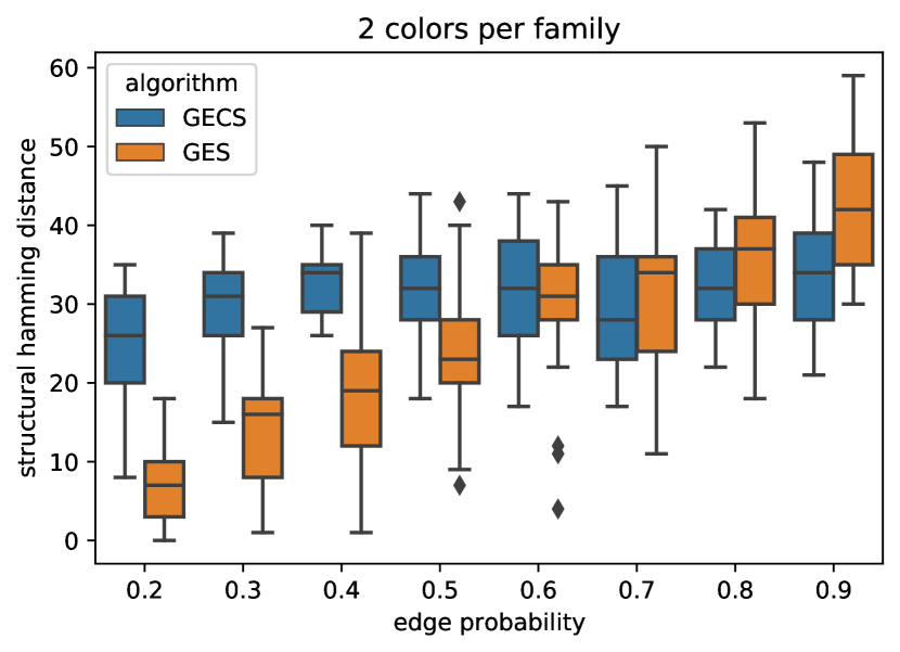
(a) $\texttt{nc}=2$

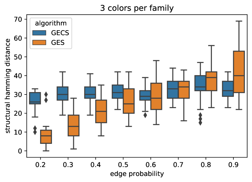
(b) $\texttt{nc}=3$

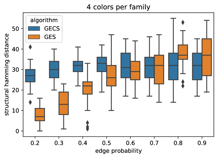
(c) $\texttt{nc}=4$

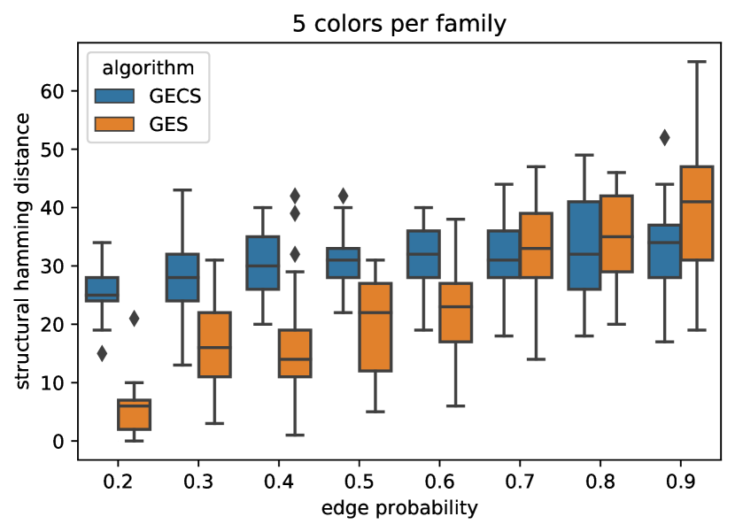
(d) $\texttt{nc}=5$

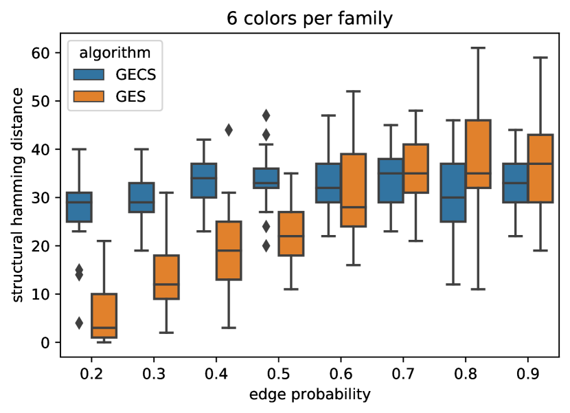
(e) $\texttt{nc}=6$

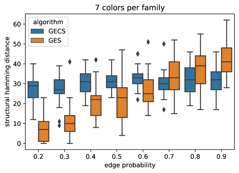
(f) $\texttt{nc}=7$

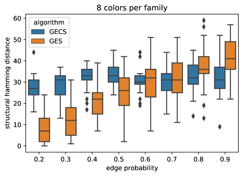
(g) $\texttt{nc}=8$

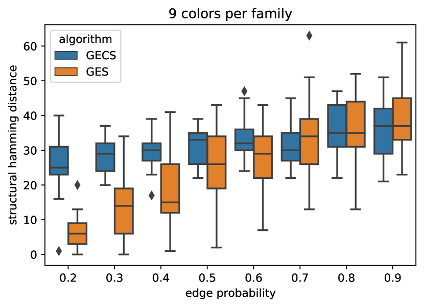
(h) $\texttt{nc}=9$

Figure 1. Structural Hamming distance results for $p=10$ and $n=250$ samples. nc is the pre-specified number of colors per family for the data-generating models.

We see from the results presented in Figures 1 and 2 that GES tends to outperform GECS for sparse graphs, but GECS emerges as an equal or better performer as the graphs become increasingly dense. One explanation for this is that the proper-coloring constraint of needing to have at least two edges pointing into each node with nonempty parent set can increase the difficulty of the learning task for GECS when the true model is sparse. This seems reasonable given that the pairing of edges mandates additional structure GES can flexibly avoid in the sparse regime.

On the other hand, GECS appears to outperform GES when the graphs are denser, especially when there are more colors. This is likely due to the fact that GECS can include more edges at a lower penalty than GES when modeling dense systems. This is because the penalization term for GES includes the sum of $p$ and the number of edges, whereas the penalization term for GECS is only $p$ summed with the number of colors.

The results also show that the SHD appears to be relatively stable for GECS as density increases, suggesting that the coloring is helping GECS with estimation in denser models while hindering it in sparser models. As noted above, we leave the question of consistency of GECS under faithfulness open, but the empirical results here provide some supporting evidence. Namely, we see a slight decrease in the median SHD between Figures 1 and 2. This trend, as for GES, is perhaps most pronounced in the very sparse setting ($\rho=0.2)$ with few colors $\texttt{nc}=2$. While the decrease in SHD in the sparse regime for increasing sample size is more significant for GES, it may also be that GECS is consistent but converging slower due to the complexity of the additional coloring constraints and associated moves.

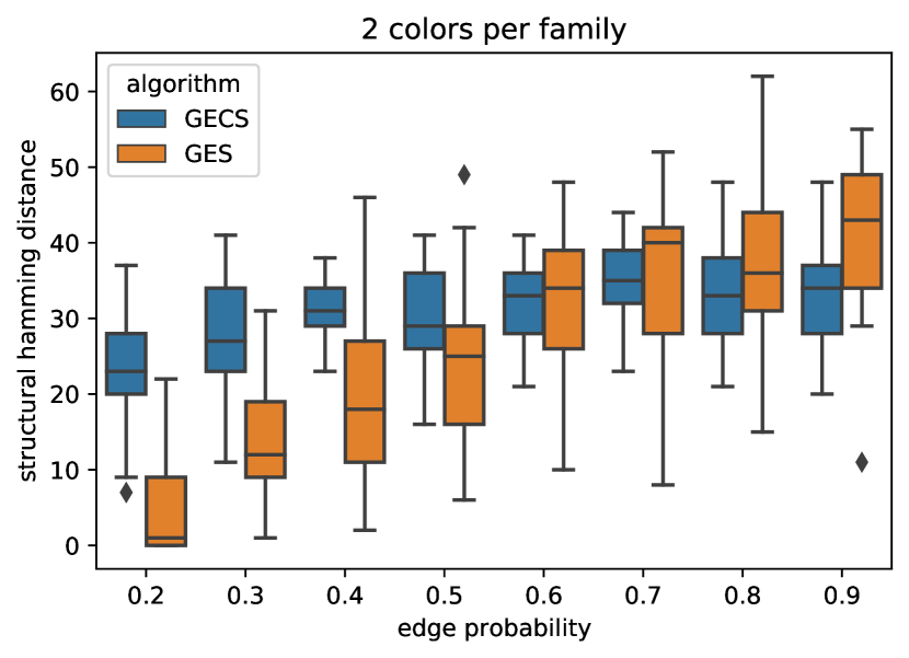
(a) $\texttt{nc}=2$

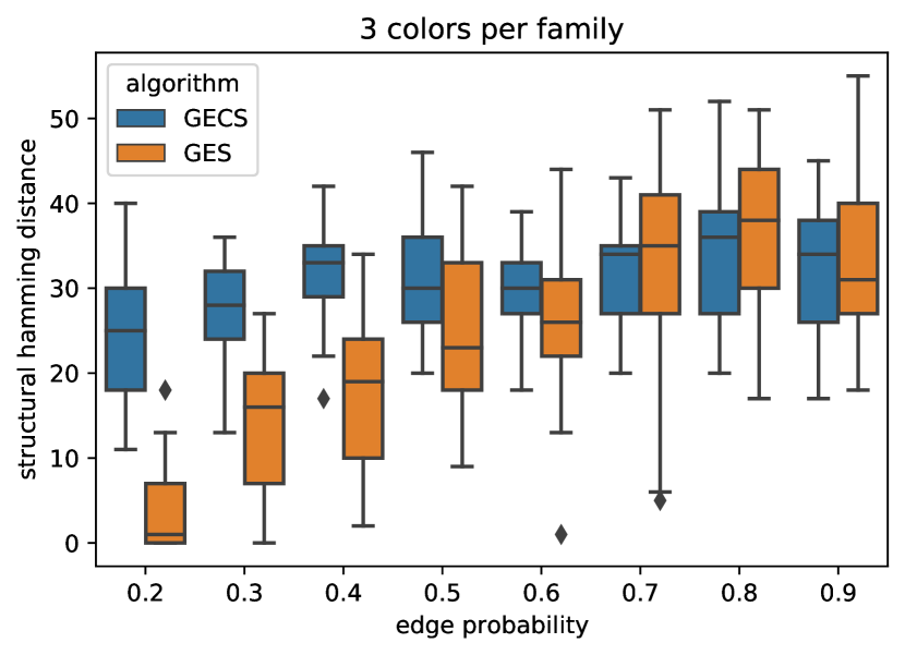
(b) $\texttt{nc}=3$

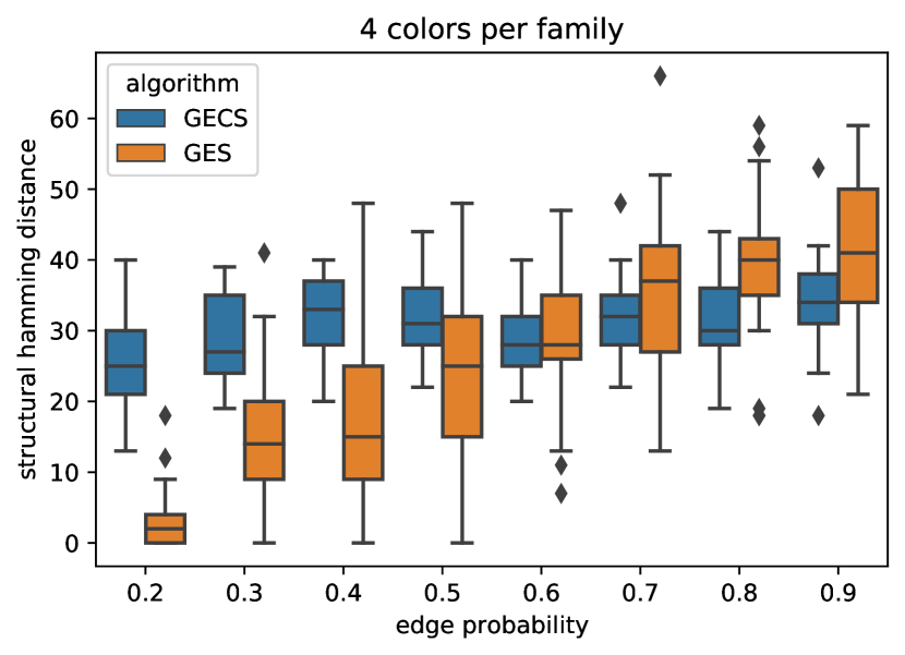
(c) $\texttt{nc}=4$

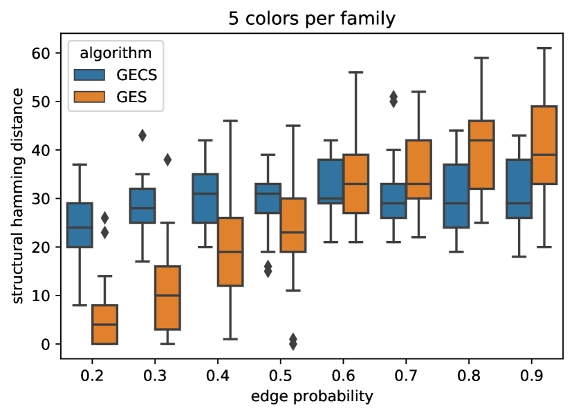
(d) $\texttt{nc}=5$

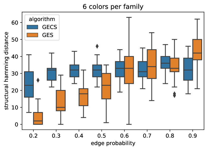
(e) $\texttt{nc}=6$

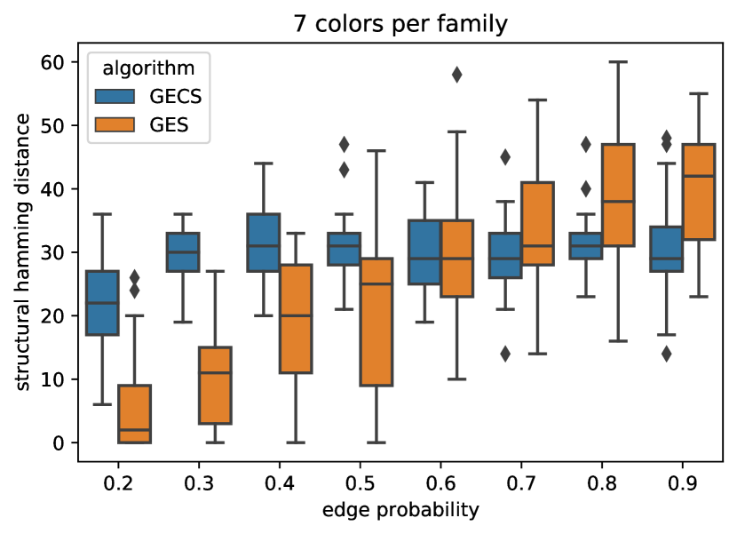
(f) $\texttt{nc}=7$

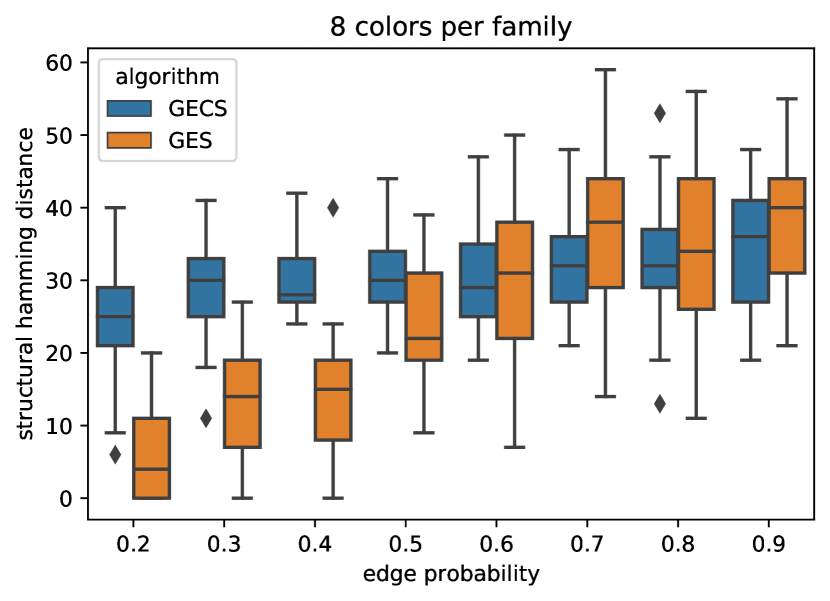
(g) $\texttt{nc}=8$

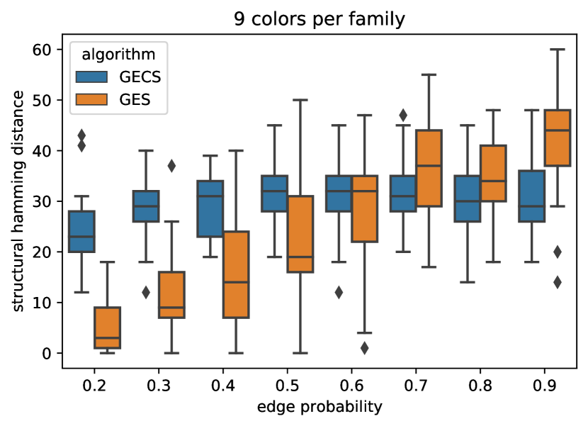
(h) $\texttt{nc}=9$

Figure 2. Structural Hamming distance results for $p=10$ and $n=1000$ samples. nc is the pre-specified number of colors per family for the data-generating models.

Overall, these observations suggest that GECS is a viable alternative for learning dense, causal DAG structures. By Theorem 5.18, the graph learned by GECS is a single DAG representing the causal system, whereas GES only learns a Markov equivalence class of possible causal DAGs. Moreover, GECS learns a BPEC-DAG, whose coloring provides additional information regarding clustering of direct causes into communities by similar causal effect. A detailed investigation into how to augment the moves used by GECS may also result in methods that still provide these additional advantages, while also beng more competitive in the sparse DAG regime.

Alternatively, generalizing Theorem 5.18 to general edge-colored DAGs, including some uncolored edges, would likely allow for adaptations of GECS that are more competitive in the sparse regime. However, the trade-off may be that the models learned are no longer structurally identifiable, as observed in Example 5.19 as well as in the partially homoscedastic (vertex-colored) setting by [WD23].

6.2. Real data experiments

We ran GECS on three real data sets. The first two data sets are the Red Wine Quality and White Wine Quality data sets available in the Wine Quality Data Set at the UCL Machine Learning Repository https://archive.ics.uci.edu/dataset/186/wine+quality. The third data set is the protein-signaling network data set of Sachs et al. [SPP${}^{+}$05].

6.2.1. Wine quality data

Each of the two data sets contains samples of $11$ physiochemical properties shared by red and white wine variants of the Portugese Vinho Verde wine which are intended for use as features in the prediction of wine quality. All variables assume numerical values on a continuous (real) domain. The red wine data set consists of 1599 joint samples of the $11$ different physiochemical properties, and the white wine data set has 4898. More details on the data can be found in [CCA${}^{+}$98]. We use GECS to give a model of the (causal) dependence structure amongst these $11$ physiochemical properties for both the red wine and white wine data sets, yielding Gaussian hierarchical models that may be used in the prediction of the overall quality of the wine.

The learned BPEC-DAGs for both wine types are presented in Figure 3. The since BPEC-DAGs are structurally identifiable, we interpret their edges causally. Indeed, we see that examples of learned arrows have believable causal meaning. For instance, the arrow from $4$ (chlorides) to $7$ (density) indicates a causal effect of chlorides on the density of the wine. Similarly, the many causal communities captured by the coloring appear to be reasonable. For example, the parents of node $5$ (free sulfur dioxide) contains the communities

$$\{0\mbox{ (fixed acidity)},1\mbox{ (volatile acidity)},2\mbox{ (citric acid)}\}\qquad\mbox{and}\qquad\{4\mbox{ (chlorides)},7\mbox{ (density)}\}.$$

The former is a collection of properties measuring acidity, so it is not unreasonable that they would have similar causal effects on free sulfur dioxide content. Similarly, chloride content and density are naturally related physiochemical properties.

(a) Red Wine

(b) White Wine

Figure 3. (a) Results for Red Wine data set. The learned BPEC-DAG has $59$ edges with $24$ color classes. (b) Results for White Wine data set. The learned BPEC-DAG has $50$ edges with $23$ color classes.

6.2.2. Protein signaling data

While GECS learned BPEC-DAG models for the wine data sets with relatively rich structure and numerous causal communities, it is also possible that BPEC-DAG models do not provide reasonable models for certain real data problems. For example, we considered the Sachs et al. data set consisting of 7644 abundance measurements of certain phospholipids and phosphoproteins present in primary human immune system cells [SPP${}^{+}$05]. The data set is purely interventional; however one may extract an observational data set consisting of $1755$ samples as described in [WSYU17, SWU20].

We ran GECS on this observational data set of 1755 samples over the $11$ measured molecules, and GECS returned the empty DAG as the optimal BPEC-DAG model. This indicates that adding even two edges with the same causal effect and head node produces a model with a lower BIC than the complete independence model. In particular, the data appears to strongly suggest that no two edges have the same causal effect in this protein-signaling network. This could be, in part, due to the fact that the data is highly non-Gaussian. However, it also seems reasonable that the causal effects among a family of variables in a protein-signaling network are vastly different for each causal relation. It is also worth considering that two causal relations in the considered protein-signaling network may have similar causal effects, but it may also be that these causal arrows do not live in the same family of variables. A generalization of GECS to all properly edge-colored DAGs may reveal such structure does indeed exist.

7. Discussion

In this paper, we considered aspects of Gaussian DAG models under the assumption of partial homogeneity constraints imposed on the vertices and edges of the DAG (i.e., the error variances and structural coefficients, respectively). Using the graphical representation of such constraints via colored DAGs introduced in [MRS22], we investigated fundamental properties of these models for their use in graphical modeling inference tasks. To embed the colored DAG representation of such models into the theory of DAG models and their many generalizations in the graphical models literature, we described both a local and global Markov property for colored Gaussian DAG models, and showed that their fulfillment is equivalent to containment in the model.

We observed fundamental geometric properties of these models, including smoothness which is useful for likelihood ratio testing [Drt09]. We also gave a proof of an algebraic conjecture of Sullivant [Sul18] by showing that the conjectured condition holds more generally in the context of colored Gaussian DAG models. Our method of proof relies on a short lemma that applies to other well-studied Gaussian graphical models for which the conjectured condition was of interest, including colored (and uncolored) undirected Gaussian graphical models as well as ancestral Gaussian graphical models. This lemma is seen to be generally applicable to parametrized statistical models admitting global rationally identifiable parameters. It would be interesting to investigate the broader implication of these techniques in settings where one wishes to identify model-defining constraints, such as in the evolutionary biology literature [AR07, CFS11].

We further investigated fundamental properties of the colored DAG models for use in causal discovery, including faithfulness and structural identifiability. We observed that generic distributions in vertex-colored and edge-colored DAG models are faithful to their defining DAGs and colorings. However, we also observed that faithfulness may breakdown for general colorings. As faithfulness is typically used as a first benchmark consistency guarantee for causal discovery algorithms, it would be useful to characterize the colored DAG models admitting faithful distributions.

We additionally provide some first structural identifiability results for models with partially homogeneous structural coefficients in the form of the family of BPEC-DAGs. These models allow for structure identification, but also provide additional information on how the direct causes of each node in the system may be clustered into communities of variables having similar causal effects on their target node. We observed some evidence of this behavior in the real data studies for the GECS causal discovery algorithm, which we introduced as an analogue of GES for learning BPEC-DAGs. In simulated data, we observed that GECS appears to outperform GES at learning dense causal DAGs, while offering the additional benefits of causal community identification and structurally identifiable DAG estimates.

We leave open the question of consistency of GECS under faithfulness. It would also be interesting to see if the structural identifiability results generalize to all properly edge-colored DAG models, or even to provide a characterization of model equivalence for general edge-colored DAG models. Given such results, GECS could be extended to these domains, where its performance in the sparse regime may be expected to improve. Here, characterizations of model equivalence that are both constraint-based (in the style of Verma and Pearl [VP90a]) as well as transformational (as considered by Chickering for DAGs [Chi13]) may be of use in formulating a version of Meek’s Conjecture [Chi02] for colored DAGs whose eventual proof could yield consistency results. Given a complete characterization of the colored DAGs admitting faithful distributions, one may even consider extensions of these investigations for general colored DAG models.

Acknowledgements

We thank Mathias Drton, Lisa Nicklasson, and Seth Sullivant for helpful discussions. Part of this research was performed while the authors were visiting the Institute for Mathematical and Statistical Innovation (IMSI), which is supported by the National Science Foundation (Grant No. DMS-1929348). Tobias Boege and Kaie Kubjas were partially supported by the Academy of Finland grant number 323416. Tobias Boege and Liam Solus were partially supported by the Wallenberg Autonomous Systems and Software Program (WASP) funded by the Knut and Alice Wallenberg Foundation. Pratik Misra received funding from the Brummers and Partners MathDataLab and the European Research Council (ERC) under the European Union’s Horizon 2020 research and innovation programme (grant agreement No. 883818) during the course of this project. Liam Solus was further supported by a Research Pairs grant from the Digital Futures Lab at KTH, the Göran Gustafsson Stiftelse Prize for Young Researchers, and Starting Grant No. 2019-05195 from The Swedish Research Council (Vetenskapsrådet).

Appendix A Proof of Theorem 3.4

We first give a self-contained proof of Lemma 3.2 which is the basis of our parameter identification results.

Proof A.1 (Proof of Lemma 3.2).

As consequences of the trek rule, we have $\Sigma_{\RM{pa}(i),i}=\Sigma_{\RM{pa}(i)}\Lambda_{\RM{pa}(i),i}$ as well as $\sigma_{ii}=\omega_{ii}+\Lambda_{i,\RM{pa}(i)}\Sigma_{\RM{pa}(i)}\Lambda_{\RM{pa}(i),i}$. Using the former to replace $\Lambda_{\RM{pa}(i),i}$ in the latter and rearranging terms yields

$$\omega_{ii}=\sigma_{ii}-\Sigma_{i,\RM{pa}(i)}\Sigma_{\RM{pa}(i)}^{-1}\Sigma_{\RM{pa}(i),i}=\frac{|\Sigma_{\RM{pa}(i)\cup i}|}{|\Sigma_{\RM{pa}(i)}|},$$

by Schur’s formula.

Suppose that $i\not\in\RM{pa}(j)$, so $\lambda_{ij}=0$. In this case, the directed local Markov property of $G$ dictates that $\CI{i,j|\RM{pa}(j)}$ holds for $\Sigma$ and hence the numerator in ($\lambda$) vanishes as required. Now suppose that $i\in\RM{pa}(j)$. As above, the trek rule in matrix form reads $\Sigma_{\RM{pa}(j),j}=\Sigma_{\RM{pa}(j)}\Lambda_{\RM{pa}(j),j}$. This implies that $\lambda_{ij}$ is the $i$-th entry of $\Sigma_{\RM{pa}(j)}^{-1}\Sigma_{\RM{pa}(j),j}$, i.e.,

$$\lambda_{ij} =(\Sigma_{\RM{pa}(j)}^{-1}\Sigma_{\RM{pa}(j),j})_{i}=\frac{(-1)^{i}}{|\Sigma_{\RM{pa}(j)}|}\sum_{s\in\RM{pa}(j)}(-1)^{s}|\Sigma_{is|\RM{pa}(j)\setminus is}|\sigma_{sj}$$

$$=\frac{(-1)^{i}}{|\Sigma_{\RM{pa}(j)}|}\left((-1)^{i}|\Sigma_{\RM{pa}(j)\setminus i}|\sigma_{ij}+\sum_{s\in\RM{pa}(j)\setminus i}(-1)^{s}|\Sigma_{is|\RM{pa}(j)\setminus is}|\sigma_{sj}\right).$$

The factors $|\Sigma_{is|\RM{pa}(j)\setminus is}|$ appearing in every term of the summation are minors with rows $\RM{pa}(j)\setminus s$ and columns $\RM{pa}(j)\setminus i$. In particular, they all contain row $i$ since $s\not=i$. In the next step, we write out the Laplace expansions of all of these minors by row $i$. To avoid confusion about signs, we use the symbol $i[K]$ to denote the position (starting with $1$) of the element $i$ in the ordered set $K$. Continuing with the expansion,

$$\lambda_{ij} =\begin{multlined}\frac{(-1)^{i[\RM{pa}(j)]}}{|\Sigma_{\RM{pa}(j)}|}\Bigg{(}(-1)^{i[\RM{pa}(j)]}|\Sigma_{\RM{pa}(j)\setminus i}|\sigma_{ij}\\ {}+\sum_{s\in\RM{pa}(j)\setminus i}(-1)^{s[\RM{pa}(j)]}\sigma_{sj}\sum_{t\in\RM{pa}(j)\setminus i}(-1)^{i[\RM{pa}(j)\setminus s]+t[\RM{pa}(j)\setminus i]}|\Sigma_{\RM{pa}(j)\setminus is,\RM{pa}(j)\setminus it}|\sigma_{it}\Bigg{)},\end{multlined}\frac{(-1)^{i[\RM{pa}(j)]}}{|\Sigma_{\RM{pa}(j)}|}\Bigg{(}(-1)^{i[\RM{pa}(j)]}|\Sigma_{\RM{pa}(j)\setminus i}|\sigma_{ij}\\ {}+\sum_{s\in\RM{pa}(j)\setminus i}(-1)^{s[\RM{pa}(j)]}\sigma_{sj}\sum_{t\in\RM{pa}(j)\setminus i}(-1)^{i[\RM{pa}(j)\setminus s]+t[\RM{pa}(j)\setminus i]}|\Sigma_{\RM{pa}(j)\setminus is,\RM{pa}(j)\setminus it}|\sigma_{it}\Bigg{)},$$

and the double sum simplifies to

$$\sum_{s,t\in\RM{pa}(j)\setminus i}(-1)^{s[\RM{pa}(j)]+i[\RM{pa}(j)\setminus s]+t[\RM{pa}(j)\setminus i]}\sigma_{it}|\Sigma_{st|\RM{pa}(j)\setminus i}|\sigma_{sj}.$$

The sign $(-1)^{i[\RM{pa}(j)\setminus s]}$ equals $(-1)^{i[\RM{pa}(j)]}$ if $s>i$ and $(-1)^{i[\RM{pa}(j)]+1}$ if $s<i$. The sign $(-1)^{s[\RM{pa}(j)]}$ equals $(-1)^{s[\RM{pa}(j)\setminus i]}$ if $s<i$ and $(-1)^{s[\RM{pa}(j)\setminus i]+1}$ if $s>i$. In both cases, their product equals $(-1)^{i[\RM{pa}(j)]+s[\RM{pa}(j)\setminus i]+1}$. Hence we have

$$\lambda_{ij} =\begin{multlined}\frac{(-1)^{i[\RM{pa}(j)]}}{|\Sigma_{\RM{pa}(j)}|}\Bigg{(}(-1)^{i[\RM{pa}(j)]}|\Sigma_{\RM{pa}(j)\setminus i}|\sigma_{ij}\\ {}-(-1)^{i[\RM{pa}(j)]}\sum_{s,t\in\RM{pa}(j)\setminus i}(-1)^{s[\RM{pa}(j)\setminus i]+t[\RM{pa}(j)\setminus i]}\sigma_{it}|\Sigma_{st|\RM{pa}(j)\setminus i}|\sigma_{sj}\Bigg{)}\end{multlined}\frac{(-1)^{i[\RM{pa}(j)]}}{|\Sigma_{\RM{pa}(j)}|}\Bigg{(}(-1)^{i[\RM{pa}(j)]}|\Sigma_{\RM{pa}(j)\setminus i}|\sigma_{ij}\\ {}-(-1)^{i[\RM{pa}(j)]}\sum_{s,t\in\RM{pa}(j)\setminus i}(-1)^{s[\RM{pa}(j)\setminus i]+t[\RM{pa}(j)\setminus i]}\sigma_{it}|\Sigma_{st|\RM{pa}(j)\setminus i}|\sigma_{sj}\Bigg{)}$$

$$=\frac{1}{|\Sigma_{\RM{pa}(j)}|}\left(|\Sigma_{\RM{pa}(j)\setminus i}|\left(\sigma_{ij}-\Sigma_{i,\RM{pa}(j)\setminus i}\Sigma_{\RM{pa}(j)\setminus i}^{-1}\Sigma_{\RM{pa}(j)\setminus i,j}\right)\right),$$

which is the claimed expression by Schur’s formula.

We now turn to Theorem 3.4. Part (1) is proved already in [WD23, Theorem 3.3]. Part (2) concerns identifying $\lambda_{ij}=0$ if $ij\not\in E$. The function $\lambda_{ij|A}(\Sigma)$ vanishes if and only if its numerator $|\Sigma_{ij|A\setminus i}|$ does. This is equivalent to the conditional independence $\CI{i,j|A\setminus i}$ which is in turn characterized by d-separation in $G$ by the global Markov property. This proves claim (2). The remainder of this section proves part (3) where we assume $ij\in E$.

Lemma A.2.

If $A\in\CC A_{G}(ij)$, then $i\in A\subseteq V\setminus\ol{\RM{de}}(j)$.

Proof A.3.

Suppose first that $A$ does not contain $i$. To show that $A$ cannot be identifying, it suffices to find one point $\Sigma=\phi_{G}(\Omega,\Lambda)\in\CC M_{G}$ such that $\lambda_{ij|A}(\Sigma)\not=\lambda_{ij}$. Since $i\not\in A$, the numerator equals $|\Sigma_{ij|A}|$ and $\lambda_{ij|A}(\Sigma)$ is exactly the Schur complement

$$\sigma_{ij}-\Sigma_{i,A}\Sigma_{A}^{-1}\Sigma_{A,j}.$$

We set all $\Lambda$-parameters except for $\lambda_{ij}$ to zero. This gives a matrix $\Sigma=\phi_{G}(\Omega,\lambda_{ij})$. Since $\Sigma_{A,j}=0$ as a result of there being no treks between $A$ and $j$, the expression for $\lambda_{ij|A}$ simplifies to $\sigma_{ij}=\lambda_{ij}\omega_{i}$ which differs from $\lambda_{ij}$.

If $j\in\ol{\RM{de}}(j)$ is in $A$, then the numerator $|\Sigma_{ij|A\setminus i}|$ has a repeated column and must vanish. However, generically $\lambda_{ij}\not=0$ on the model. Finally suppose that $A$ contains a descendant $k\in\ol{\RM{de}}(j)\setminus j$. We may pick the smallest such $k$ in $A$. Again, it suffices to find one point on which the identification of $\lambda_{ij}$ fails. Let $p$ be a directed path from $j$ to $k$. By setting all $\Lambda$-parameters outside of $p$ except for $\lambda_{ij}$ to zero (which disconnects all vertices not on this path), we see that it is sufficient to prove the statement for the path $i\to j\to k_{1}\to\dots\to k_{n}=k$ with $\Set{i,k}\subseteq A\subseteq\Set{i,k_{1},\dots,k_{n}}$. Since all $k_{i}$ are descendants of $j$ and $k$ is the smallest descendant of $j$ in $A$, we have $A=\Set{i,k}$. The statement that $A$ is edge-identifying is equivalent to the vanishing of the polynomial expression in $2\times 2$ determinants:

$$|\Sigma_{ij|k}|-\lambda_{ij}|\Sigma_{ik}| =\begin{vmatrix}\sigma_{ij}&\sigma_{ik}\\ \sigma_{jk}&\sigma_{kk}\end{vmatrix}-\lambda_{ij}\begin{vmatrix}\sigma_{ii}&\sigma_{ik}\\ \sigma_{ik}&\sigma_{kk}\end{vmatrix}.$$

There is a unique trek between $i$ and every other vertex on the path and its top node is $i$. Between $j$ and its descendant $k$ there are exactly two treks, one with top $i$ and one with top $j$. We have $\sigma_{jk}=\left(\lambda_{ij}+\frac{\omega_{j}}{\sigma_{ij}}\right)\sigma_{ik}$. Thus

$$\begin{vmatrix}\sigma_{ij}&\sigma_{ik}\\ \sigma_{jk}&\sigma_{kk}\end{vmatrix}-\lambda_{ij}\begin{vmatrix}\sigma_{ii}&\sigma_{ik}\\ \sigma_{ik}&\sigma_{kk}\end{vmatrix} =\sigma_{ij}\sigma_{kk}-\sigma_{ik}^{2}\left(\lambda_{ij}+\frac{\omega_{j}}{\sigma_{ij}}\right)-\lambda_{ij}\left(\omega_{i}\sigma_{kk}-\sigma_{ik}^{2}\right)$$

$$=-\frac{\omega_{j}}{\omega_{i}\lambda_{ij}}\sigma_{ik}^{2}.$$

This is the negative product of the trek monomials from $i$ to $k$ and from $j$ to $k$. For generic choices of parameters, neither of them is zero.

Recall from the statement of Theorem 3.4 that for a DAG $G=(V,E)$ with $ij\in E$, we denote by $G_{ij}$ the induced subgraph of $G$ in which the edge $i\to j$ and all descendants of $j$ are removed.

Lemma A.4.

Let $A$ be a d-separating set for $i$ and $j$ in $G_{ij}$. Then $A\cup i\in\CC A_{G}(ij)$.

Proof A.5.

Let $\Sigma=\phi_{G}(\Omega,\Lambda)\in\CC M_{G}$ be arbitrary. The graph $G_{ij}$ arises from $G$ by deleting edge $ij$ and descendants of $j$. This corresponds to setting some $\Omega$ and $\Lambda$ parameters to zero. Taking the leftover parameters through the parametrization $\phi_{G_{ij}}$ results in a matrix $\Sigma^{\prime}\in\CC M(G_{ij})$. By assumption $|\Sigma^{\prime}_{ij|A}|=0$. The submatrices $\Sigma_{ij|A}$ and $\Sigma^{\prime}_{ij|A}$ are very similar:

• Since $j$ is a sink node in the induced subgraph of $G$ on vertices $ijA$, no descendant of $j$ establishes a new trek among any of the vertices in $ijA$.

• The presence of the edge $ij$ is the only other difference between the graphs. Again, since $j$ is a sink in $ijA$, the only entries of $\Sigma_{ij|A}$ that differ from $\Sigma^{\prime}_{ij|A}$ are: $\sigma_{ij}=\sigma^{\prime}_{ij}+\lambda_{ij}\sigma^{\prime}_{ii}$ and $\sigma_{jk}=\sigma^{\prime}_{jk}+\lambda_{ij}\sigma^{\prime}_{ik}$, for $k\in A$.

This shows that the $j$-column of $\Sigma_{ij|A}$ is just $\Sigma_{iA,j}=\Sigma^{\prime}_{iA,j}+\lambda_{ij}\Sigma^{\prime}_{iA,i}$. Hence, by multilinearity of the determinant:

$$|\Sigma_{ij|A}|=\underbrace{|\Sigma^{\prime}_{ij|A}|}_{=0}+\lambda_{ij}|\Sigma_{iA}|,$$

which establishes identifiability.

Lemma A.6.

Let $A$ be a d-connecting set for $i$ and $j$ in $G_{ij}$. Then $A\cup i\not\in\CC A_{G}(ij)$.

Proof A.7.

As in the proof of Lemma A.2, it suffices to find a matrix $\Sigma$ in the model (or any submodel) where $\lambda_{ij|A}(\Sigma)\not=\lambda_{ij}$. For any set $A$ which d-connects $i$ and $j$ in $G_{ij}$, we get a supporting undirected path in $G_{ij}$. We set all edge parameters outside of this path and except for $\lambda_{ij}$ to zero. This gives a sequence of treks $i\leftarrow\dots\leftarrow t_{1}\to\dots\to c_{1}\leftarrow\dots\leftarrow t_{2}\to\dots\to c_{2}\leftarrow\dots\to c_{m}\leftarrow\dots\leftarrow t_{m+1}\to\dots\to j$ which are glued together at colliders $c_{1},\dots,c_{m}$. The set $A$ consisting of these colliders is the only set which d-connects $i$ and $j$ in this graph. Hence, in this special case — which covers every d-connection statement in $G_{ij}$ — it suffices to only treat $A=\Set{c_{1},\dots,c_{m}}$. In the subgraph of $G$ which we consider, only the edge $ij$ is added to this gluing of treks.

Suppose first that $m=0$, so that we have a simple trek $i\leftarrow\dots\leftarrow t\to\dots\to j$ and $A=\emptyset$. Then $|\Sigma_{ij|A}|=\lambda_{ij}\sigma_{ii}+\omega_{t}\lambda^{\tau}=\lambda_{ij}|\Sigma_{i}|+\omega_{t}\lambda^{\tau}$, where $\tau$ is the trek from $i$ to $j$ over $t$. Generically, $\omega_{t}\lambda^{\tau}\not=0$, so $A=\emptyset$ is not identifying.

In case $m>0$, we can deduce the following facts from the structure of the graph:

• $\Sigma_{A}$ is a tridiagonal matrix.

• In $\Sigma_{i,A}$ the only nonzero entry is $\sigma_{ic_{1}}$.

• In $\Sigma_{A,j}$ the only nonzero entries are $\sigma_{c_{1}j}$ and $\sigma_{c_{m}j}$.

• We have $\sigma_{ij}=\lambda_{ij}\sigma_{ii}$ and $\sigma_{c_{1}j}=\lambda_{ij}\sigma_{c_{1}i}$.

Using multilinearity of the determinant in the $j$-column of $|\Sigma_{ij|A}|$ shows

Itsuffi

References

- [AHDLP24] Félix Almendra-Hernández, Jesús A De Loera and Sonja Petrović: Irreducible markov chains on spaces of graphs with fixed degree-color sequences. arXiv preprint arXiv:2402.09568 (2024).
- [AMP97] Steen A. Andersson, David Madigan and Michael D. Perlman: A characterization of Markov equivalence classes for acyclic digraphs. Ann. Stat., 25(2):505–541 (1997). doi: https://doi.org/10.1214/aos/1031833662.
- [AR07] Elizabeth S Allman and John A Rhodes: Phylogenetic invariants. Reconstructing evolution: new mathematical and computational advances, pp. 108–146 (2007).
- [BKKR23] Tobias Boege, Thomas Kahle, Andreas Kretschmer and Frank Röttger: The geometry of gaussian double markovian distributions. Scandinavian Journal of Statistics, 50(2):665–696 (2023). doi: https://doi.org/10.1111/sjos.12604.
- [CCA98] P. Cortez, A. Cerdeira, F. Almeida, T. Matos and J. Reis: Modeling wine preferences by data mining from physicochemical properties. Decision Support Systems, 47(4):547–553 (1998).
- [CFS11] Marta Casanellas and Jesús Fernández-Sánchez: Relevant phylogenetic invariants of evolutionary models. Journal de mathématiques pures et appliquées, 96(3):207–229 (2011).
- [Chi02] David Maxwell Chickering: Optimal structure identification with greedy search. Journal of machine learning research, 3(Nov):507–554 (2002).
- [Chi13] David Maxwell Chickering: A transformational characterization of equivalent bayesian network structures. arXiv preprint arXiv:1302.4938 (2013).
- [Drt09] Mathias Drton: Likelihood ratio tests and singularities. Ann. Stat., 37(2):979–1012 (2009). doi: https://doi.org/10.1214/07-AOS571.
- [Drt18] Mathias Drton: Algebraic problems in structural equation modeling. In The 50th anniversary of Gröbner bases, vol. 77, pp. 35–87. Mathematical Society of Japan (2018).
- [DRW20] Mathias Drton, Elina Robeva and Luca Weihs: Nested covariance determinants and restricted trek separation in Gaussian graphical models. Bernoulli, 26(4):2503–2540 (2020). doi: https://doi.org/10.3150/19-BEJ1179.
- [DX10] Mathias Drton and Han Xiao: Smoothness of Gaussian conditional independence models. In Algebraic methods in statistics and probability II. AMS special session algebraic methods in statistics and probability, March 27–29, 2009, University of Illinois at Urbana-Champaign, Champaign, Il, USA., pp. 155–177. American Mathematical Society (AMS) (2010).
- [FMW85] Stephen E Fienberg, Michael M Meyer and Stanley S Wasserman: Statistical analysis of multiple sociometric relations. Journal of the american Statistical association, 80(389):51–67 (1985).
- [GP74] Victor Guillemin and Alan Pollack: Differential topology. Prentice-Hall (1974).
- [HB12] Alain Hauser and Peter Bühlmann: Characterization and greedy learning of interventional markov equivalence classes of directed acyclic graphs. The Journal of Machine Learning Research, 13(1):2409–2464 (2012).
- [HJ13] Roger A. Horn and Charles R. Johnson: Matrix analysis. Cambridge University Press, 2nd ed. ed. (2013).
- [HJM08] Patrik Hoyer, Dominik Janzing, Joris M Mooij, Jonas Peters and Bernhard Schölkopf: Nonlinear causal discovery with additive noise models. Advances in neural information processing systems, 21 (2008).
- [HL08] Søren Højsgaard and Steffen L. Lauritzen: Graphical Gaussian models with edge and vertex symmetries. J. R. Stat. Soc., Ser. B, Stat. Methodol., 70(5):1005–1027 (2008). doi: https://doi.org/10.1111/j.1467-9868.2008.00666.x.
- [HLL83] Paul W Holland, Kathryn Blackmond Laskey and Samuel Leinhardt: Stochastic blockmodels: First steps. Social networks, 5(2):109–137 (1983).
- [Kem11] Gregor Kemper: A course in commutative algebra, vol. 256 of Graduate Texts in Mathematics. Springer (2011). doi: https://doi.org/10.1007/978-3-642-03545-6.
- [KF09] Daphne Koller and Nir Friedman: Probabilistic graphical models: principles and techniques. MIT press (2009).
- [KPP24] Vishesh Karwa, Debdeep Pati, Sonja Petrović, Liam Solus, Nikita Alexeev, Mateja Raič, Dane Wilburne, Robert Williams and Bowei Yan: Monte carlo goodness-of-fit tests for degree corrected and related stochastic blockmodels. Journal of the Royal Statistical Society Series B: Statistical Methodology, 86(1):90–121 (2024).
- [Lau96] Steffen L Lauritzen: Graphical models, vol. 17. Clarendon Press (1996).
- [MDLW18] Marloes Maathuis, Mathias Drton, Steffen Lauritzen and Martin Wainwright: Handbook of graphical models. CRC Press (2018).
- [Mee95] C Meek: Strong completeness and faithfulness in bayesian networks. In Proc. Conf. on Uncertainty in Artificial Intelligence (UAI-95), pp. 411–418 (1995).
- [MRS22] Visu Makam, Philipp Reichenbach and Anna Seigal: Symmetries in directed gaussian graphical models (2022). arXiv:2108.10058 [math.ST].
- [PB14] Jonas Peters and Peter Bühlmann: Identifiability of Gaussian structural equation models with equal error variances. Biometrika, 101(1):219–228 (2014).
- [Pea09] Judea Pearl: Causality. Models, reasoning, and inference. Cambridge, 2nd revised ed. ed. (2009).
- [PJS17] Jonas Peters, Dominik Janzing and Bernhard Schölkopf: Elements of causal inference: foundations and learning algorithms. The MIT Press (2017).
- [PMJS12] Jonas Peters, Joris Mooij, Dominik Janzing and Bernhard Schölkopf: Identifiability of causal graphs using functional models. UAI 2011, Proceedings of the Twenty-Seventh Conference on Uncertainty in Artificial Intelligence, Barcelona, Spain, July 14-17, 2011, p. 589–598 (2012).
- [RP14] Hajir Roozbehani and Yury Polyanskiy: Algebraic methods of classifying directed graphical models (2014). arXiv:1401.5551 [cs.IT].
- [RS02] Thomas Richardson and Peter Spirtes: Ancestral graph markov models. The Annals of Statistics, 30(4):962–1030 (2002).
- [SG91] Peter Spirtes and Clark Glymour: An algorithm for fast recovery of sparse causal graphs. Social science computer review, 9(1):62–72 (1991).
- [SGS00] Peter Spirtes, Clark N Glymour and Richard Scheines: Causation, prediction, and search. MIT press (2000).
- [SHH06] Shohei Shimizu, Patrik O Hoyer, Aapo Hyvärinen, Antti Kerminen and Michael Jordan: A linear non-gaussian acyclic model for causal discovery. Journal of Machine Learning Research, 7(10) (2006).
- [Shi14] Shohei Shimizu: Lingam: Non-gaussian methods for estimating causal structures. Behaviormetrika, 41(1):65–98 (2014).
- [SPP05] Karen Sachs, Omar Perez, Dana Pe’er, Douglas A Lauffenburger and Garry P Nolan: Causal protein-signaling networks derived from multiparameter single-cell data. Science, 308(5721):523–529 (2005).
- [SRM98] Peter Spirtes, Thomas Richardson, Christopher Meek, Richard Scheines and Clark Glymour: Using path diagrams as a structural equation modeling tool. Sociological Methods & Research, 27(2):182–225 (1998). doi: https://doi.org/10.1177/0049124198027002003.
- [STD10] Seth Sullivant, Kelli Talaska and Jan Draisma: Trek separation for Gaussian graphical models. Ann. Stat., 38(3):1665–1685 (2010). doi: https://doi.org/10.1214/09-AOS760.
- [Sul08] Seth Sullivant: Algebraic geometry of gaussian bayesian networks. Adv. Appl. Math., 40(4):482–513 (2008). doi: https://doi.org/10.1016/j.aam.2007.04.004.
- [Sul18] Seth Sullivant: Algebraic Statistics, vol. 194 of Graduate Studies in Mathematics. American Mathematical Society (AMS) (2018).
- [SWU20] Chandler Squires, Yuhao Wang and Caroline Uhler: Permutation-based causal structure learning with unknown intervention targets. In Conference on Uncertainty in Artificial Intelligence, pp. 1039–1048. PMLR (2020).
- [SWU21] Liam Solus, Yuhao Wang and Caroline Uhler: Consistency guarantees for greedy permutation-based causal inference algorithms. Biometrika, 108(4):795–814 (2021).
- [Usm94] Riaz A. Usmani: Inversion of a tridiagonal Jacobi matrix. Linear Algebra and its Applications, 212-213:413–414 (1994). doi: https://doi.org/10.1016/0024-3795(94)90414-6.
- [VP90a] Thomas S. Verma and Judea Pearl: Causal networks: Semantics and expressiveness. In Ross D. Shachter, Tod S. Levitt, Laveen N. Kanal and John F. Lemmer, eds.: Uncertainty in Artificial Intelligence, vol. 9 of Machine Intelligence and Pattern Recognition, pp. 69–76. North-Holland (1990). doi: https://doi.org/10.1016/B978-0-444-88650-7.50011-1.
- [VP90b] Thomas S. Verma and Judea Pearl: Equivalence and synthesis of causal models. In Proceedings of the Sixth Annual Conference on Uncertainty in Artificial Intelligence, UAI ’90, pp. 255–270. Elsevier (1990).
- [WD23] Jun Wu and Mathias Drton: Partial homoscedasticity in causal discovery with linear models. IEEE Journal on Selected Areas in Information Theory (2023).
- [WSYU17] Yuhao Wang, Liam Solus, Karren Yang and Caroline Uhler: Permutation-based causal inference algorithms with interventions. Advances in Neural Information Processing Systems, 30 (2017).
- [YKU18] Karren Yang, Abigail Katcoff and Caroline Uhler: Characterizing and learning equivalence classes of causal dags under interventions. In International Conference on Machine Learning, pp. 5541–5550. PMLR (2018).