Unified equations of state for cold nonaccreting neutron stars with Brussels-Montreal functionals. V. Improved parametrization of the nucleon density distributions

Abstract

We previously studied the inner crust and the pasta mantle of a neutron star within the 4th-order extended Thomas-Fermi (ETF) approach with consistent proton shell corrections added perturbatively via the Strutinsky integral (SI) theorem together with the contribution due to pairing. To speed up the computations and avoid numerical problems, we adopted parametrized nucleon density distributions. However, the errors incurred by the choice of the parametrization are expected to become more significant as the mean baryon number density is increased, especially in the pasta mantle where the differences in the energy per nucleon of the different phases are very small, typically a few keV. To improve the description of these exotic structures, we discuss the important features that a nuclear profile should fulfill and introduce two new parametrizations. Performing calculations using the BSk24 functional, we find that these parametrizations lead to lower ETF energy solutions for all pasta phases than the parametrization we adopted before and more accurately reproduce the exact equilibrium nucleon density distributions obtained from unconstrained variational calculations. Within the ETFSI method, all parametrizations predict the same composition in the region with quasi-spherical clusters. However, the two new parametrizations lead to a different mantle structure at mean baryon densities above about $0.07$ fm^-3, at which point lasagna is energetically favored. Interestingly, spherical clusters reappear in the pasta region. The inverted pasta phases such as bucatini and Swiss cheese are still found in the densest region above the core in all cases.

I Introduction

After its birth in a gravitational core-collapse supernova explosion, a neutron star (NS) rapidly cools down. After several weeks Pons and Viganò (2019), the region with mean baryon number densities $\bar{n}$ below about half-saturation density $n_{0}$ crystallizes. This solid crust consists of a crystal lattice of spherical or quasi-spherical neutron-rich nuclei embedded in a relativistic electron gas coexisting with free neutrons in its inner part. The core of the star remains a homogeneous liquid made of nucleons and leptons, and possibly other particles in the densest part (see, e.g., Ref. Blaschke and Chamel (2018) for a recent review). At the interface between the crust and the core, peculiar structures collectively referred to as ‘nuclear pasta’ could emerge Hashimoto et al. (1984); Ravenhall et al. (1983). The existence of such a mantle would affect neutrino emission (see, e.g., Refs. Gusakov et al. (2004); Lin et al. (2020)), electron transport important for thermal and electrical conductivities (see, e.g., Refs. Yakovlev (2015); Pelicer et al. (2023)), bulk viscosity Yakovlev et al. (2018) and elastic properties Pethick and Potekhin (1998); Caplan et al. (2018); Pethick et al. (2020); Zemlyakov and Chugunov (2023) of dense matter. This nuclear-pasta mantle could therefore be relevant to various NS phenomena.

This paper is a continuation of our recent work on the structure of the nuclear-pasta mantle Pearson et al. (2020); Pearson and Chamel (2022); Shchechilin et al. (2023), in which we extended a semi-microscopic treatment originally developed for ordinary nuclei Dutta et al. (1986) and later adapted to the inner crust of a NS Dutta et al. (2004); Onsi et al. (2008); Pearson et al. (2012, 2015, 2018). Our framework is based on the ETFSI approach, a computationally very fast approximation to the Hartree-Fock-Bogoliubov (HFB) calculations using semi-local functionals, such as those constructed from effective interactions of the Skyrme type. It is a two-stage method in which one first performs extended Thomas-Fermi (ETF) calculations, followed by the addition of shell effects through the application of the Strutinsky Integral (SI) theorem, and the inclusion of pairing either via the Bardeen-Cooper-Schrieffer (BCS) method or the local-density approximation. Both these corrections are made in a manner consistent with the ETF first stage.

The ETF method Kirzhnits (1967); Grammaticos and Voros (1979, 1980); Brack et al. (1985) gives an approximation to the kinetic-energy density $\tau_{q}(\boldsymbol{r})$ and the spin current $\boldsymbol{J_{q}}(\boldsymbol{r})$ in the functional. It consists in expanding the Bloch density matrix in powers of $\hbar$ Wigner (1932); Kirkwood (1933), thereby enabling $\tau_{q}(\boldsymbol{r})$ and $\boldsymbol{J_{q}}(\boldsymbol{r})$ to be expressed as functions entirely of the nucleon densities $n_{q}(\boldsymbol{r})$ and their gradients Brack et al. (1985) (the highest degree of the derivatives corresponds to the order of expansion); the fourth-order terms are necessary for an accurate reproduction of the nuclear binding energies Pi et al. (1988); Centelles et al. (1990). In this way, the energy becomes a functional of only the nucleon density distributions, and it is these, rather than wavefunctions, that are treated as the basic variables in a full Euler-Lagrange (EL) minimization for a given mean baryon number density $\bar{n}$. It was shown that the nucleon densities $n_{q}(\boldsymbol{r})$ that satisfy the EL equations are smooth functions Barkat et al. (1972). Assuming that pasta forms periodic structures, it is enough to calculate the energy of a single Wigner-Seitz (WS) cell of the corresponding crystal lattice with a given number $Z$ of protons and $N$ of neutrons ($Z$ and $N$ represent the numbers per unit length in the case of spaghetti and bucatini, and the numbers per unit area for lasagna). Such a cell is a truncated octahedron for a body-centered cubic crystal of quasi-spherical clusters or bubbles (Swiss cheese), an infinitely long regular hexagonal prism for a hexagonal lattice of spaghetti or bucatini, and an infinitely long right prism for lasagna. The EL equations have to be solved with periodic boundary conditions, a consequence of which is that the gradient of the nucleon densities along directions perpendicular to the WS cell faces must vanish  Wigner and Seitz (1933).

A full EL minimization is challenging, particularly for the three-dimensional case of quasi-spherical clusters and bubbles, and also for the two-dimensional case of spaghetti or bucatini, since in both cases the EL equations are reduced to partial differential equations. For this reason, the WS cell is generally approximated by more symmetrical cells of equal mean nucleon densities: a spherically symmetric sphere in the former case (this approximation was originally introduced by Wigner and Seitz in the context of electrons in solids Wigner and Seitz (1933)), and an axially symmetric cylinder in the latter case. For lasagna, no approximation is needed, except that we assume it to be invariant under space inversion, thus ensuring a consistent treatment of all geometries. Then, the smoothness requirement of the nucleon distributions together with the periodicity lead to the boundary conditions

$$\dfrac{dn_{q}}{d\xi}(\xi=0)=\dfrac{dn_{q}}{d\xi}(\xi=R)=0\quad,$$ (1)

where $\xi$ is the radial coordinate for the spherical and cylindrical cells of radius $R$ and the Cartesian coordinate perpendicular to the plates of half-size $R$ in case of lasagna.

Even though the EL method has been reduced to a one-dimensional problem, solving the ordinary differential equations that have replaced the partial differential equations can still cause significant numerical problems, especially with the full implementation of the ETF method up to the fourth order Brack et al. (1985). In all our previous applications of the ETFSI method, the calculations were greatly simplified and computationally speeded up by parametrizing the nucleon density distributions. Without any loss of generality, the nucleon profiles can be conveniently expressed as

$${n_{q}}(\xi,\mathbf{x})=n_{\mathrm{B}q}+n_{\Lambda q}f_{q}(\xi,\bm{\chi})\quad.$$ (2)

The parameter set $\mathbf{x}$ thus includes the background density $n_{\mathrm{B}q}$ and the parameter $n_{\Lambda q}$ that modulates the density excess or deficit due to the presence of clusters or holes respectively. The remaining parameters $\bm{\chi}$ are contained in the smooth dimensionless function $f_{q}(\xi,\bm{\chi})$ describing the spatial inhomogeneities. Once the form of this function has been chosen the parameter set $\mathbf{x}$ for the given values of $N$ and $Z$ is determined by minimizing the total ETF energy per nucleon, which includes not only the nuclear energy but also the energy of the neutralizing electron gas and of the Coulomb lattice Pearson et al. (2018, 2020).

With the ETF part of the ETFSI calculation completed, microscopic corrections due to proton shell effects are added, as described in Ref. Pearson and Chamel (2022). The analogous corrections for neutrons are expected to be negligible because of the occupation of (quasi)continuum states Oyamatsu and Yamada (1995); Chamel (2006); Chamel et al. (2007). For consistency, we drop the shell correction when the Fermi energy exceeds the value of the potential at the border of the cell. Here we ignore proton pairing since its impact was shown to be quite marginal in the pasta mantle Pearson and Chamel (2022); Shchechilin et al. (2023). Neutron pairing effects will be the subject of a future study.

The main concern of this paper is with the choice of a smooth profile function $f_{q}(\xi,\bm{\chi})$. In the original application of the ETFSI method to finite nuclei (for which $n_{\mathrm{B}q}=0$), the simple Fermi-Dirac distribution was adopted Dutta et al. (1986),

$$f^{\mathrm{FD}}_{q}(\xi)=\frac{1}{1+\exp\Big{(}\frac{\xi-C_{q}}{a_{q}}\Big{)}}\quad,$$ (3)

where $C_{q}$ is the half-width nuclear radius and $a_{q}$ accounts for the diffuseness of the the nuclear surface. This form has also been recently employed for ETFSI calculations of the inner crust of a NS Shelley and Pastore (2021). However, the parametrization (3) (like the majority of those employed for ordinary nuclei, e.g. Refs.  Bethe (1968); Brueckner et al. (1969); Moszkowski (1970); Blaizot and Grammaticos (1981); Kolehmainen et al. (1985)) does not appear to be very well suited in this context since it does not satisfy the boundary conditions (1). The associated errors can be significant, especially in the pasta region where the size of the clusters or holes is comparable to the distance between them.

For this reason, the following modification was proposed in Ref. Onsi et al. (2008) and adopted in all our subsequent studies including Refs. Pearson et al. (2020); Pearson and Chamel (2022); Shchechilin et al. (2023):

$$f^{\mathrm{StrD}}_{q}(\xi)=\frac{1}{1+\exp\left[\Big{(}\frac{C_{q}-R}{\xi-R}\Big{)}^{2}-1\right]\exp\Big{(}\frac{\xi-C_{q}}{a_{q}}\Big{)}}\quad.$$ (4)

The additional exponential factor ensures that not only the first derivative of ${n_{q}}(\xi,\mathbf{x})$ vanishes at the border of the cell but in fact that all derivatives do so. The vanishing of the first three derivatives makes possible a substantial simplification of the 4th-order ETF expressions for the energy by integrating by parts Brack et al. (1985); Onsi et al. (1997). However, the vanishing of all derivatives on the cell surface leads inevitably to a strong damping with a very flat tail. Moreover, this profile, like the Fermi profile (3), has the further defect of a kink at the origin, i.e., a non-zero first derivative. Evaluating the impact of these limitations in the parametrization (4) and investigating the necessary improvements constitute the objective of this paper.

In Section II.1, we introduce two new parametrizations for the nucleon density distributions and we show in Section II.2 that they lead to a more accurate description of nuclear pasta by performing ETF calculations with functional BSk24. Complete ETFSI calculations with these new profile functions are presented and discussed in Section III. Our conclusions are given in Section IV.

II Optimization of nuclear profiles

II.1 Choice of profiles

Besides being a smooth function, satisfying the boundary conditions (1), the parametrization should be flexible enough to describe not only phases with clusters immersed in a more dilute medium but also inverted phases such as bucatini and Swiss cheese. The case of lasagna is peculiar in that the distinction between these two different topologies vanishes: although a configuration with a ‘hole’ at the center of the cell appears as an anti-lasagna, it can be transformed into a lasagna by a simple translation, as illustrated by the green dash-dotted line in Fig. 1. In other words, these two seemingly different configurations are physically identical. To avoid introducing a spurious distinction between lasagna and anti-lasagna, both should be describable equally well by the chosen parametrization. This means that for any given profile $n_{q}(\xi,\bf{x})$, there should exist a set of parameters $\bf{x^{\prime}}$ such that the inverted profile ${n_{q}}(R-\xi,\mathbf{x^{\prime}})$ obtained from a space inversion followed by a translation is also allowed, as shown in Fig. 1:

$${n_{q}}(\xi,\mathbf{x})={n_{q}}(R-\xi,\mathbf{x^{\prime}})\,.$$ (5)

This condition guarantees that these lasagna and anti-lasagna configurations have the same energy. Even though this argument is not applicable in the case of spheres and cylinders because of the WS approximation, there are still reasons why Eq. (5) would be desirable in those cases. Indeed, the condition (5) ensures equal treatment of spheres (spaghetti) and Swiss cheese (bucatini) since for any profile obtained for the former, the inverted one will be also allowed for the latter. The strong damping parametrization does not satisfy this requirement, thus leading to an artificial anti-lasagna configuration. Moreover, it can only describe ‘flat-bottom’ spheres and ‘flat-top’ bubbles, as illustrated in Fig. 2 by the solid green and dashed blue lines respectively. But ‘flat-bottom’ Swiss cheese (corresponding to the red dash-dotted line) are not allowed. The same limitation applies to the spaghetti and bucatini shapes.

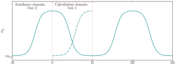
Figure 1: Illustration of the identity between the seemingly different lasagna (green solid line) and anti-lasagna (green dash-dotted line) configurations in the calculation domain (dotted red box). These configurations are actually not physically distinct since the anti-lasagna profile can be obtained from a space inversion followed by a translation of the lasagna profile. This symmetry leads to the condition (5).

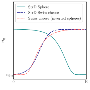
Figure 2: Schematic picture illustrating possible nucleon distributions inside the WS cell using the StrD parametrization (2) and (4): ‘flat-bottom’ spheres (green solid line) and ‘flat-top’ Swiss cheese (blue dashed line). The ‘flat-bottom’ Swiss cheese profile (red dash-dotted line) obtained from the inversion of spheres cannot be described by this parametrization (see text for discussion).

To improve the description of pasta and assess the sensitivity of our results with respect to the choice of the parametrization, we first consider the ‘3FD’ parametrization consisting of a combination of three Fermi-Dirac functions (3) as follows:

$$f^{\mathrm{3FD}}_{q}(\xi)=f^{\mathrm{FD}}_{q}(-\xi)+f^{\mathrm{FD}}_{q}(\xi)+f^{\mathrm{FD}}_{q}(2R-\xi)+C^{\mathrm{3FD}}\quad,$$ (6)

where the constant $C^{\mathrm{3FD}}=f^{\mathrm{FD}}_{q}(-R)+2f^{\mathrm{FD}}_{q}(R)$ is added so that $f_{q}(R)=0$. Raising the Fermi-Dirac distributions to the power $\gamma$ (see, e.g., Refs. Kolehmainen et al. (1985); Brack et al. (1985)) does not lead to a substantial energy reduction in the pasta region (as was also found in Ref. Martin and Urban (2015)), therefore we set $\gamma=1$ here. Apart from all the advantages of the simple Fermi-Dirac form, e.g. fulfilling the condition (5) with $n_{\Lambda q}^{\prime}=-n_{\Lambda q}$, $a_{q}^{\prime}=a_{q}$, and $C_{q}^{\prime}=R-C_{q}$, and $n_{{\rm B}q}^{\prime}=n_{{\rm B}q}+n_{\Lambda q}(3+C^{\rm fd}+C^{\rm fd\,\prime})$, the additional merit is that this parametrization is smoother although the first derivatives at $\xi=0$ and $\xi=R$ are still not strictly zero.

On the other hand the satisfaction of the boundary condition (1) can be exactly achieved by generalizing the strong-damping expression (4) to

$$f^{\mathrm{}}_{q}(\xi)=\frac{1}{1+h(\xi;C_{q},a_{q})\exp\Big{(}\frac{\xi-C_{q}}{a_{q}}\Big{)}}\quad,$$ (7)

in which the function $h(\xi;C_{q},a_{q})$ ensures the fulfillment of the conditions (1). Moreover, if the function is such that

$$h(\xi;C_{q},a_{q})=\frac{1}{h(R-\xi;R-C_{q},a_{q})}\quad,$$ (8)

it follows that the constraint (5) can be easily satisfied with $n_{\Lambda q}^{\prime}=-n_{\Lambda q}$, $n_{{\rm B}q}^{\prime}=n_{{\rm B}q}+n_{\Lambda q}$, $a_{q}^{\prime}=a_{q}$, and $C_{q}^{\prime}=R-C_{q}$. The simplest function $h(\xi;C_{q},a_{q})$ that we have found obeying these requirements is:

$$h(\xi;C_{q},a_{q})=\left(\frac{C_{q}-R}{C_{q}}\right)^{2}\left(\frac{\xi}{\xi-R}\right)^{2}\quad.$$ (9)

Only the first derivative of this new profile, which we will refer to as ‘SoftD’ below, vanishes on the cell surface. This SoftD profile therefore allows for a softer damping than the StrD profile (4).

II.2 Results of ETF minimization

To optimize the minimization of the ETF energy, we start the calculations in the shallowest layers of the inner crust containing quasi-spherical nuclei for which fairly accurate initial guesses for the parameters of the profiles can be set: $C_{q}\approx 6$ fm, $a_{q}\approx 0.5$ fm, $n_{\Lambda n}\approx N/(\frac{4}{3}\pi C_{n}^{3})$ and $n_{\Lambda p}\approx Z/(\frac{4}{3}\pi C_{p}^{3})$. The final values are then taken as initial guesses for the deeper neighboring layer. The process is repeated until the crust-core boundary is reached. We have checked the robustness of our results by varying the initial guesses at different densities. It is important to scan regions of parameter space large enough to ensure that our minima are true minima minimora, and not just local minima.

We now compare the results obtained with the three profile parametrizations. The StrD profile (4), which we implemented in our previous works and, as was mentioned earlier, involves an integrated version of the fourth-order ETF method  Brack et al. (1985); Onsi et al. (1997), is used as a reference. In addition, we consider the two new profiles 3FD (6) and SoftD (7), (9) for which we use full ETF expressions for $\tau_{q}(\boldsymbol{r})$ and $\boldsymbol{J_{q}}(\boldsymbol{r})$ given in Refs. Grammaticos and Voros (1979, 1980); Bartel and Bencheikh (2002), since only the first derivatives at $\xi=0$ and $\xi=R$ vanish. In this case, the only price to pay is a slight increase in the computational time.

Since the ETF approach is completely variational, it is this method that should serve as a basis for choosing the optimal parametrization. To this end, we minimize the energy per nucleon for each of the three parametrizations considering the five different phases: spheres, spaghetti, bucatini, lasagna, and Swiss cheese. Figure 3 shows the corresponding energy per nucleon with the energy for spheres subtracted. The corresponding equilibrium pasta configurations are indicated by the color bar at the bottom of each panel. The results for the StrD are identical to the ones presented in Ref. Shchechilin et al. (2023). The most remarkable difference obtained with the two new profiles is the reappearance of lasagna between the spaghetti and bucatini phases. The onset of the pasta phases is slightly shifted from $\bar{n}_{\mathrm{sp}}\approx 0.05\,\text{fm}^{-3}$ for StrD to $\bar{n}_{\mathrm{sp}}\approx 0.052-0.053\,\text{fm}^{-3}$ for the two new profiles. The crust-core transition density is barely affected, being $\bar{n}_{\mathrm{cc}}\approx 0.082\,\text{fm}^{-3}$. It corresponds to the point, for which the energy of the densest pasta phase, namely the Swiss cheese for all profiles, is equal to the energy of uniform $npe$ matter (characterized by $n_{\mathrm{\Lambda}q}=0$). Within the same nuclear functional, the compressible liquid drop model can yield a similar pasta sequence, but only if the curvature correction is included Dinh Thi et al. (2021); Zemlyakov et al. (2021).

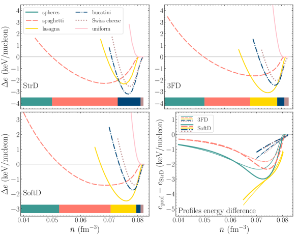
Figure 3: (upper panels and lower left panel) Energy per nucleon of different pasta phases minus the energy per nucleon of spheres within the ETF approach versus the mean baryon density for the three adopted parametrizations of the nucleon profiles. Orange dashed lines correspond to spaghetti, solid yellow to lasagna, navy dash-dotted to bucatini, brown dotted to Swiss cheese, and solid pink to uniform $npe$ matter. The equilibrium shape is illustrated by the bars at the bottom of the panels with the same color coding. (lower right panel) The energy difference between the two new profiles and StrD Onsi et al. (2008) for various pasta shapes. Solid green lines are added for spheres. The thin lines represent the 3FD profile and the thick ones are for the SoftD, while colors and line styles are the same as in the two upper panels and lower left one.

To better understand these results, we demonstrate in the bottom right panel of Fig. 3 the energy per nucleon of each phase obtained with the two new parametrizations after subtracting out the energy per nucleon for StrD. It is clear that in all cases the new parametrizations yield lower energies. In general, SoftD performs slightly better than 3FD for the clusterized phases, while 3FD is preferred for the inverted phases. The energy differences amount to a maximum of about $\approx 2-3$ keV per nucleon for spheres and spaghetti and is reached near $\bar{n}\approx 0.074\,\text{fm}^{-3}$. For the inverted phases at the relevant densities, the energy reduction with the new parametrizations does not exceed $\approx 1$ keV per nucleon. The largest deviations of order $\lesssim 4-5$ keV per nucleon are found in the lasagna phase and are enough to change the sequence of pasta.

As an illustrative example, we plot in Fig. 4 the equilibrium nucleon distributions in the WS cell at $\bar{n}=0.074\,\text{fm}^{-3}$ for the three different parameterizations. The two new SoftD and 3FD profiles vary more smoothly than StrD and lead to smaller cells. The difference is again more prominent for the lasagna phase, complementing the conclusions of Fig. 3. In addition, we show in Appendix A that the two new profiles (unlike StrD) are flexible enough to reproduce the EL solutions in the TF approximation obtained in Ref. Sharma et al. (2015). This suggests that 3FD and SoftD distributions lie very close to the exact profiles and are preferred to the StrD.

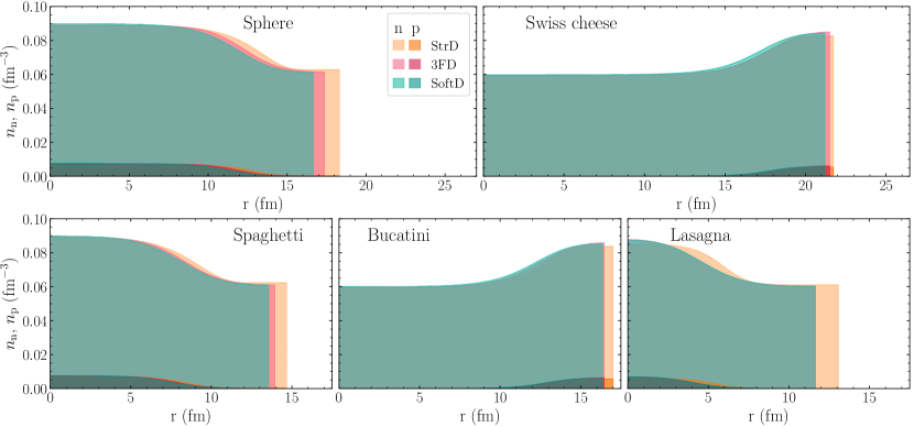
Figure 4: Equilibrium nucleon density profiles for three parametrizations at $\bar{n}=0.074\,\text{fm}^{-3}$. Green shading corresponds to SoftD, pink for 3FD, and orange for StrD. Proton distributions are plotted with darker colors than neutrons.

III Results of full ETFSI calculations

At the next step following the approach of Refs.Pearson and Chamel (2022); Shchechilin et al. (2023), we add the SI corrections on top of the ETF energy per nucleon for each of the three profile parametrizations StrD, 3FD, and SoftD. In the low-density layers of the inner crust, clusters are quasi-spherical and sufficiently far apart so that the differences in the profiles at the ETF level turn out to be insignificant (see also Fig. 3). Moreover, the proton shell effects are more pronounced leading to deeper local minima in the ETFSI energy per nucleon. Consequently, all the profile parametrizations predict the same composition.

However, in the deeper region of the pasta mantle at densities above $\approx 0.06$ fm^-3, the choice of the parametrization matters. In Fig. 5, we display the ETFSI results over the whole density range of pasta phases for the three adopted parametrizations. As found earlier in Refs. Pearson and Chamel (2022); Shchechilin et al. (2023), the spaghetti phase predicted at the ETF level totally disappears when the SI correction is added for all three parametrizations (only the configurations with dripped protons appear in the scale of Fig. 5 beyond $\bar{n}\approx 0.067\,\text{fm}^{-3}$). As a consequence, the spherical clusters remain present at higher densities thus shrinking the pasta mantle substantially. In contrast to the StrD, the SoftD, and the 3FD parametrizations lead to the presence of lasagna in the density range $\bar{n}_{\mathrm{sp}}\approx 0.07\,\text{fm}^{-3}-0.08\,\text{fm}^{-3}$. Interestingly, this layer occurs to be interspersed by spheres around $\bar{n}\approx 0.075\,\text{fm}^{-3}$. The existence of the same pasta phases in different regions of a NS was previously discussed in Ref. Magierski and Heenen (2002). Beyond $\bar{n}_{\mathrm{drip}}\approx 0.078\,\text{fm}^{-3}$, some protons become unbound for all considered shapes, and since we then drop the SI corrections, the presence of bucatini and Swiss cheese as well as the crust-core transition are unaffected. As shown in Fig. 5, the total ETFSI results for the two new parametrizations are quite the same.

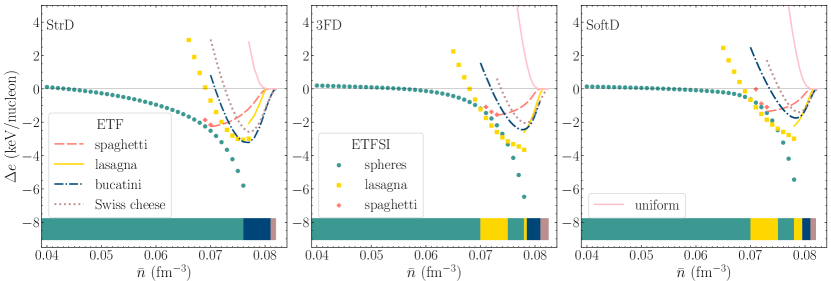
Figure 5: ETFSI and ETF energy per nucleon for different pasta phases minus the ETF energy per nucleon for spheres versus mean baryon density for the three considered profile parametrizations. The ETFSI results for spheres (solid green circles) and lasagna (solid yellow squares) are supplemented with ETF results (the same as in Fig. 3) beyond proton drip for the corresponding phase. For spaghetti, all configurations shown (solid pluses - ETFSI, dashed lines - ETF) are beyond proton drip (see text for details). For completeness, the ETF energies per nucleon for bucatini and Swiss cheese and the results for the homogeneous nuclear matter are plotted (see also Fig. 3). Color bars at the bottom indicate the equilibrium phases.

To analyse in more detail the role of the initial ETF parametrizations, we fix the density to $\bar{n}=0.065\,\text{fm}^{-3}$ and plot the energies per particle as a function of $Z$ in Fig. 6. For spheres, a typical shell structure is found for all parametrizations with a sharp minimum at $Z=40$. In the case of spaghetti and lasagna, the energy per nucleon also exhibits some smooth fluctuations with $Z$ associated with the filling of levels (see also Ref. Oyamatsu and Yamada (1995)). In Ref. Pearson and Chamel (2022), the interval of the $Z$ considered was too small to reveal these fluctuations. The SI correction for spaghetti leads to a substantial reduction of $Z$ by more than a factor of 2, from $Z_{\mathrm{eq}}\approx 1.4$ fm^-1 to $Z_{\mathrm{eq}}\approx 0.6$ fm^-1. For such small values of $Z_{\mathrm{eq}}$, the SI correction is reduced but at the cost of increasing the ETF energy. The end result is that the ETFSI energy per nucleon is larger than for spheres and lasagna (note the different scales in Fig. 6) leading to the vanishing of spaghetti. As discussed in Appendix B, this can be understood from the different filling of energy levels.

Comparing the results obtained for the three different parametrizations, the StrD is found to yield the highest ETFSI energy per nucleon for all phases. As discussed before, the energy reduction with the new parametrizations has the biggest impact on the lasagna phase. The SoftD and 3FD lead to remarkably close predictions. Notably, it can also be seen that differences in the energy per nucleon among the three parametrizations tend to be reduced when the SI correction is added. Nevertheless, differences still exist, especially between the StrD and the two new parametrizations. This is due to the perturbative nature of the corrections.

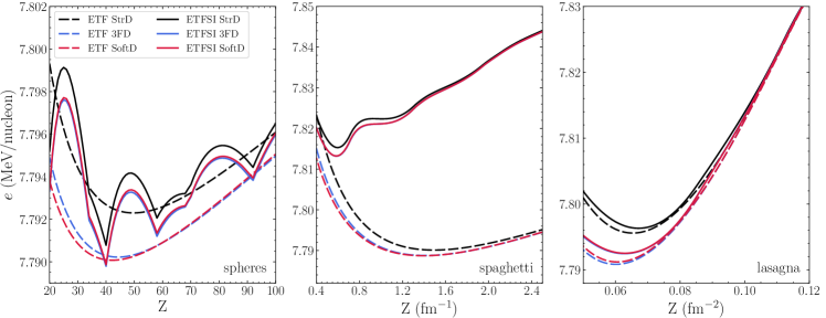
Figure 6: ETF (dashed lines) and ETFSI (solid lines) energies per nucleon versus proton number for spheres, proton number per unit length for spaghetti and proton number per unit area for lasagna at baryon density $\bar{n}=0.065\,\text{fm}^{-3}$. Three different parametrizations of the nucleon density distributions were considered: 3FD (blue lines), SoftD (red lines), StrD (black lines).

These results are also reflected in the proton density distributions plotted in Fig. 7. There the parametrized ETF profiles are compared to those calculated in the ETFSI approach (for the corresponding optimal $Z$ value that is different from that in the ETF calculation) by summing the occupied single-particle wave functions obtained from the solutions of the HF equations with the ETF mean fields. The effect of the SI corrections is the most significant for spaghetti and can be traced back to the drop of $Z$. For spheres, the ETFSI treatment induces quantum fluctuations inside the cluster. For lasagna, the initial parametrized profiles can already be considered as a fairly good approximation to the ETFSI profiles (see also Appendix A for further comparisons).

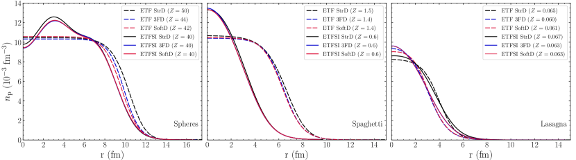
Figure 7: Proton density distributions profiles, as obtained within the ETFSI (solid lines) or ETF (dashed lines) method, for spheres, spaghetti, and lasagna at $\bar{n}=0.065\,\text{fm}^{-3}$. Red lines correspond to SoftD, blue for 3FD, and black for StrD. Each profile is plotted for its own optimum $Z$ value (see Fig. 6).

IV Conclusions

We have determined the structure of the deepest layers of the inner crust and of the pasta mantle of a NS within the ETFSI approach, investigating the role of the parametrization of the nucleon distributions. To this end, we have formulated the requirements that the profiles should satisfy. (i) The first derivatives should vanish at the center and at the border of the WS cell, as expressed in Eq. (1). (ii) The profile should satisfy Eq. (5) to avoid introducing an artificial distinction between lasagna and anti-lasagna. (iii) The parametrization should be flexible enough to reproduce as closely as possible the exact profiles obtained from the solutions of the EL equations. We have shown that the various parametrizations employed for isolated nuclei (in vacuum) Brueckner et al. (1969); Bethe (1968); Brack et al. (1985); Kolehmainen et al. (1985); Moszkowski (1970); Blaizot and Grammaticos (1981) and even the ones specifically developed for the inner crust (including ours) Oyamatsu (1993); Gögelein and Müther (2007); Martin and Urban (2015); Lim and Holt (2017); Mondal et al. (2020); Onsi et al. (2008); Pearson et al. (2018) have several drawbacks limiting their reliability, especially in the pasta layers. For this reason, we have introduced the parametrizations SoftD and 3FD (see Eqs. (2), (7), (9), and (6)), fulfilling the aforementioned requirements.

First, we have compared at the ETF level these two new parametrizations with the StrD parametrization we proposed in Ref. Onsi et al. (2008). For numerical calculations, we have applied the generalized Skyrme functional BSk24 Goriely et al. (2013) as in our recent series of works Pearson et al. (2018, 2020); Pearson and Chamel (2022); Shchechilin et al. (2023). We have found that the Soft and 3FD parametrizations yield lower energies for all pasta phases, notably for lasagna. This shows that the new parametrizations are more realistic, leading to configurations that are more stable and therefore closer to the exact EL solutions. The obtained energy reductions are substantial to alter the equilibrium structure of the pasta mantle. Namely, in contrast to the StrD parametrization, the SoftD and 3FD parametrizations lead to the same traditional sequence of pasta with increasing density, as predicted by most CLD models : spheres, spaghetti, lasagna, bucatini, and Swiss cheese.

When including the SI corrections, all three parametrizations agree in their predictions up to the point where pasta appears, at densities $\bar{n}_{\mathrm{sp}}\approx 0.07\,\text{fm}^{-3}$. This transition density is significantly increased compared to the ETF results. This is caused by the vanishing of spaghetti as we previously found in Refs. Pearson and Chamel (2022); Shchechilin et al. (2023) using the StrD parametrization. This stems from the fact that the SI correction is large and positive, which in turn arises because of a comparatively larger number of protons occupying the most loosely bound levels (see Fig. 9). Despite the tendency of the SI correction to compensate the differences in the ETF energy from initially parametrized profiles, the StrD results differ from the two new parametrizations at densities above $\bar{n}_{\mathrm{sp}}\approx 0.07\,\text{fm}^{-3}$. In this region, both the SoftD and 3FD parametrizations predict lasagna to be present, which is, surprisingly, interspersed among spherical clusters. In all cases, the densest layers of the pasta mantle consist of inverted phases, namely bucatini and Swiss cheese, and the transition to the homogeneous core occurs at $\bar{n}_{\mathrm{cc}}\approx 0.082\,\text{fm}^{-3}$. The end result is that the pasta mantle calculated with the two new parameterizations has a more complicated structure and extends over a slightly wider range of densities than obtained with the StrD, though considerably reduced compared to ETF results. All in all, the new proposed nuclear profile parametrizations yield similar results, predicting a pasta mantle structure closer to the true equilibrium. These parameterizations are therefore more realistic and better suited for investigating the role of different nuclear functionals in the formation of nuclear pasta.

Appendix A Flexibility of the profile parametrizations

Here we provide a simple test of the flexibility of the different parametrizations by trying to fit directly the parameters to realistic nuclear profiles in the NS mantle (without performing the ETF(SI) minimization). For this purpose, we have taken the nucleon density distributions obtained in Ref. Sharma et al. (2015) from the solution of the EL equations within the TF approximation at different mean baryon densities. We also include in the analysis the profiles from self-consistent HF calculations of the lasagna phase for the fixed proton fraction $Y_{\mathrm{p}}=0.1$ and $\bar{n}=0.04$ fm^-3 Sekizawa et al. (2022). For the sake of completeness, in addition to the parametrizations StrD, 3FD, and SoftD, we have considered the parametrization widely applied for TF calculations Oyamatsu (1993); Gögelein and Müther (2007); Miyatsu et al. (2013); Lim and Holt (2017)

$$f^{\mathrm{PW}}_{q}(\xi)=\begin{cases}\left[1-\left(\dfrac{\xi}{C_{q}}\right)^{a_{q}}\right]^{3},&r<C_{q},\\[14.22636pt] 0,&r\geq C_{q}.\end{cases}$$ (10)

Although the form (10) satisfies the boundary conditions (1), it leads to divergences for the 4-th order ETF energy. It is also clear that the condition (5) cannot be fulfilled for $C_{q}<R$.

In practice, we have fixed for each parametrization the background density and the radius of the clusters from the data and freely adjusted the remaining parameters $C_{q},a_{q}$, and $n_{\mathrm{\Lambda}q}$. The resulting fits are presented in Fig. 8. The two new parametrizations (3FD and SoftD) are able to accurately reproduce the equilibrium nucleon density distributions of Refs. Sharma et al. (2015) (although we show only the results for spherical clusters, the fits are equally good for other nuclear shapes) and Sekizawa et al. (2022). The agreement is less satisfactory for the parametrization (10), for which the variations of the neutron densities appear too sharp, especially at low densities $\bar{n}$ (see also Ref. Arponen (1972)). Although the StrD parametrization reproduces equally well the profiles for spherical clusters at low densities, the quality of the fit deteriorates with increasing density. This parametrization fails to properly describe the diffuse nuclear surface and the nuclear distributions near the border of the WS cell: imposing the vanishing of all the derivatives at $\xi=R$ appears too restrictive.

These comparisons show that the two new parametrizations SoftD and 3FD are very well suited for describing nuclear pasta. The good fits to the self-consistent HF calculations of Ref. Sekizawa et al. (2022) suggest that a fairly accurate description of lasagna could be already achieved at the ETF level.

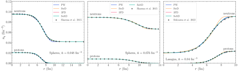
Figure 8: (left panel) Nucleon density distributions for spherical clusters at mean baryon density $\bar{n}=0.0475$ fm^-3. The results of Ref. Sharma et al. (2015) are represented by crosses, while the curves correspond to fits obtained with different parametrizations: PW (blue), StrD (orange), 3FD (pink) and SoftD (green). (middle panel) The same but for $\bar{n}=0.076$ fm^-3. (right panel) The nucleon density distributions for the lasagna phase at $\bar{n}=0.04$ fm^-3 with $Y_{\mathrm{p}}=0.1$. Crosses are results from Ref. Sekizawa et al. (2022).

Appendix B Vanishing of spaghetti

The striking conclusion of Ref. Pearson and Chamel (2022) was the complete vanishing of spaghetti within the ETFSI approach, a result confirmed here using new parametrizations of the nuclear profiles. To better understand this rather unexpected feature, we analyze more closely the role of the SI correction, focusing on the density $\bar{n}=0.065\,\text{fm}^{-3}$, for which spaghetti dominates over spheres and lasagna at the ETF level. We consider here only the SoftD parametrization. For each pasta shape, we now fix $Z$ to the optimum value obtained within the ETF approach. The proton density distributions obtained at the ETF and ETFSI levels are plotted in Fig. 9. For spheres and lasagna, results are essentially the same as in Fig. 7 since the optimum $Z$ values are hardly altered by the SI corrections. For spaghetti, however, the proton density distribution obtained at the ETFSI level is significantly different than the one shown in Fig. 7 due to the drop in $Z$ there. In particular, the distribution exhibits a bump resembling the one found in the HF+BCS calculations of Ref. Gögelein and Müther (2007). Such kind of profiles reflect the peculiarities of the single-particle wave functions of occupied proton states, which in turn are determined by the shape of the mean-field potentials. As shown in the bottom panels of Fig. 9, the potential for spaghetti is as deep as for spheres but significantly narrower although wider than for lasagna. This can be easily understood if we imagine the transformation of a spherical cluster into spaghetti or lasagna by stretching it and keeping the cell volume fixed and without changing the number of neutrons and protons (for a given mean baryon number density $\bar{n}$, the proton fraction is essentially determined by bulk properties, namely the symmetry energy, independently of the nuclear shape).

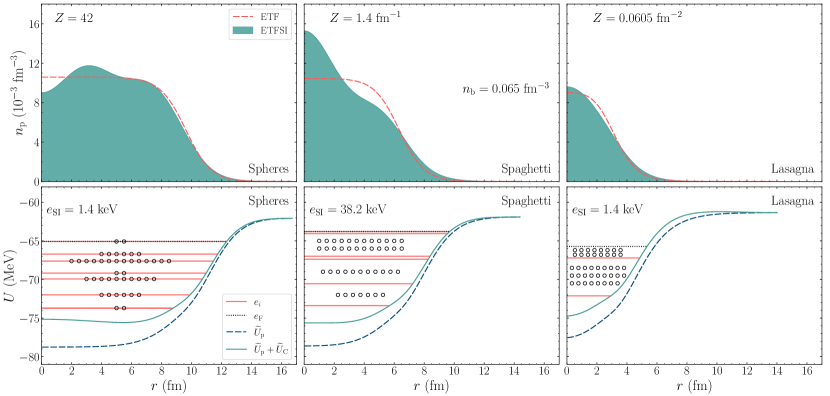
Figure 9: (top panels) Proton density distributions, as obtained within the ETFSI (filled area) or ETF (dashed lines) method, for spheres, spaghetti, and lasagna at $\bar{n}=0.065\,\text{fm}^{-3}$. (bottom panels) The central (dashed navy lines) and total (solid green) proton mean-field potential are constructed from the ETF profiles. The energy levels are shown by red lines and the Fermi energy by black dotted lines. For spheres, the appropriate number of particles on each level is placed. For spaghetti and lasagna, as energy between the levels is filled by continuum states, the ‘nominal’ number of particles between levels is shown. See text for details.

The occupied proton states are illustrated in Fig. 9. For spherical clusters, the energy of each level is discrete and can accommodate $2(2\ell+1)$ particles, where $\ell$ is the orbital quantum number (the factor of two accounts for the two possible spin projections recalling that we neglect the spin-orbit coupling). The situation is different for spaghetti and lasagna. The energy levels characterized by the set of quantum numbers $\nu$ can be written as Pearson and Chamel (2022)

$$\epsilon_{\nu}= e_{\mu}+\dfrac{\hbar^{2}k_{z}^{2}}{2m_{p}},$$ for spaghetti (11)

$$\epsilon_{\nu}= e_{\mu}+\dfrac{\hbar^{2}k_{\perp}^{2}}{2m_{p}}, \text{ for lasagna}\quad,$$ (12)

where $k_{z}=\pi n/L$ and $k_{\perp}=\pi\sqrt{n^{2}+m^{2}}/L$ are the wave numbers associated with motion along the spaghetti and in the plane of lasagna respectively ($n$ and $m$ are integers and $L$ is the size of the pasta). In both cases, $e_{\mu}$ can only take discrete values ($\mu$ represents the principal quantum number). But the energies in between are now also allowed so that the Fermi energy $\epsilon_{\mathrm{F}}$ lies above the last occupied state $\mu$. More particles can fill in the interlevel spacing for lasagna than for spaghetti due to the degeneracy with the direction of motion (see also (11)-(12)). This situation is illustrated in Fig. 9. Although the total number of protons in each phase is the same and is approximately $42$ (the length of spaghetti and the area of lasagna was set so as to obtain the same volume as for spheres), they populate only two discrete levels for lasagna, six for spaghetti and seven for spheres. On the other hand, the narrower potential for spaghetti and lasagna tends to shift the energy levels to higher values than for spheres. The relative importance of the SI correction arises from the competition between these two effects. Spaghetti is found to have the largest number of protons on the most loosely bound levels resulting in a substantially larger SI correction of $38.2$ keV per nucleon compared to 1.4 for spheres and lasagna (note that in all cases these corrections still remain very small compared to the total ETF energy per nucleon - less than $0.5\%$).

In other words, the large SI correction for spaghetti stems from the quantum mechanical necessity of fitting the bound protons inside the potential, whose shape is constrained by the minimization of the ETF energy at given mean baryon density $\bar{n}$. This analysis also suggests that the ETF approach could lead to spurious inhomogeneous configurations, which would vanish in a fully quantum mechanical treatment if the associated potential is too narrow or too shallow to contain bound energy levels Brau and Lassaut (2004).

References

- Pons and Viganò (2019) J. A. Pons and D. Viganò, Living Reviews in Computational Astrophysics 5, 3 (2019).
- Blaschke and Chamel (2018) D. Blaschke and N. Chamel, in Astrophysics and Space Science Library, edited by L. Rezzolla, P. Pizzochero, D. I. Jones, N. Rea, and I. Vidaña (2018), vol. 457 of Astrophysics and Space Science Library, p. 337.
- Hashimoto et al. (1984) M. Hashimoto, H. Seki, and M. Yamada, Progress of Theoretical Physics 71, 320 (1984).
- Ravenhall et al. (1983) D. G. Ravenhall, C. J. Pethick, and J. R. Wilson, Phys. Rev. Lett. 50, 2066 (1983).
- Gusakov et al. (2004) M. E. Gusakov, D. G. Yakovlev, P. Haensel, and O. Y. Gnedin, Astron. Astrophys. 421, 1143 (2004).
- Lin et al. (2020) Z. Lin, M. E. Caplan, C. J. Horowitz, and C. Lunardini, Phys. Rev. C 102, 045801 (2020).
- Yakovlev (2015) D. G. Yakovlev, Mon. Not. R. Astron. Soc. 453, 581 (2015).
- Pelicer et al. (2023) M. R. Pelicer, M. Antonelli, D. P. Menezes, and F. Gulminelli, Mon. Not. R. Astron. Soc. 521, 743 (2023).
- Yakovlev et al. (2018) D. G. Yakovlev, M. E. Gusakov, and P. Haensel, Mon. Not. R. Astron. Soc. 481, 4924 (2018).
- Pethick and Potekhin (1998) C. J. Pethick and A. Y. Potekhin, Physics Letters B 427, 7 (1998).
- Caplan et al. (2018) M. E. Caplan, A. S. Schneider, and C. J. Horowitz, Phys. Rev. Lett. 121, 132701 (2018).
- Pethick et al. (2020) C. J. Pethick, Z.-W. Zhang, and D. N. Kobyakov, Phys. Rev. C 101, 055802 (2020).
- Zemlyakov and Chugunov (2023) N. A. Zemlyakov and A. I. Chugunov, Universe 9, 220 (2023).
- Pearson et al. (2020) J. M. Pearson, N. Chamel, and A. Y. Potekhin, Phys. Rev. C 101, 015802 (2020).
- Pearson and Chamel (2022) J. M. Pearson and N. Chamel, Phys. Rev. C 105, 015803 (2022).
- Shchechilin et al. (2023) N. N. Shchechilin, N. Chamel, and J. M. Pearson, Phys. Rev. C 108, 025805 (2023).
- Dutta et al. (1986) A. K. Dutta, J. P. Arcoragi, J. M. Pearson, R. Behrman, and F. Tondeur, Nucl. Phys. A 458, 77 (1986).
- Dutta et al. (2004) A. K. Dutta, M. Onsi, and J. M. Pearson, Phys. Rev. C 69, 052801 (2004).
- Onsi et al. (2008) M. Onsi, A. K. Dutta, H. Chatri, S. Goriely, N. Chamel, and J. M. Pearson, Phys. Rev. C 77, 065805 (2008).
- Pearson et al. (2012) J. M. Pearson, N. Chamel, S. Goriely, and C. Ducoin, Phys. Rev. C 85, 065803 (2012).
- Pearson et al. (2015) J. M. Pearson, N. Chamel, A. Pastore, and S. Goriely, Phys. Rev. C 91, 018801 (2015).
- Pearson et al. (2018) J. M. Pearson, N. Chamel, A. Y. Potekhin, A. F. Fantina, C. Ducoin, A. K. Dutta, and S. Goriely, Mon. Not. R. Astron. Soc. 481, 2994 (2018).
- Kirzhnits (1967) D. A. Kirzhnits, Field theoretical methods in many body systems (Pergamon, Oxford, 1967).
- Grammaticos and Voros (1979) B. Grammaticos and A. Voros, Annals of Physics 123, 359 (1979).
- Grammaticos and Voros (1980) B. Grammaticos and A. Voros, Annals of Physics 129, 153 (1980).
- Brack et al. (1985) M. Brack, C. Guet, and H. B. Håkansson, Phys. Rep. 123, 275 (1985).
- Wigner (1932) E. Wigner, Physical Review 40, 749 (1932).
- Kirkwood (1933) J. G. Kirkwood, Physical Review 44, 31 (1933).
- Pi et al. (1988) M. Pi, X. Viñas, F. Garcias, and M. Barranco, Physics Letters B 215, 5 (1988).
- Centelles et al. (1990) M. Centelles, M. Pi, X. Viñas, F. Garcias, and M. Barranco, Nucl. Phys. A 510, 397 (1990).
- Barkat et al. (1972) Z. Barkat, J.-R. Buchler, and L. Ingber, Astrophys. J. 176, 723 (1972).
- Wigner and Seitz (1933) E. Wigner and F. Seitz, Phys. Rev. 43, 804 (1933).
- Oyamatsu and Yamada (1995) K. Oyamatsu and M. Yamada, in Nuclei in the Cosmos III, edited by M. Busso, C. M. Raiteri, and R. Gallino (1995), vol. 327 of American Institute of Physics Conference Series, p. 239.
- Chamel (2006) N. Chamel, Nucl. Phys. A 773, 263 (2006).
- Chamel et al. (2007) N. Chamel, S. Naimi, E. Khan, and J. Margueron, Phys. Rev. C 75, 055806 (2007).
- Shelley and Pastore (2021) M. Shelley and A. Pastore, Phys. Rev. C 103, 035807 (2021).
- Bethe (1968) H. A. Bethe, Physical Review 167, 879 (1968).
- Brueckner et al. (1969) K. A. Brueckner, J. R. Buchler, R. C. Clark, and R. J. Lombard, Physical Review 181, 1543 (1969).
- Moszkowski (1970) S. A. Moszkowski, Phys. Rev. C 2, 402 (1970).
- Blaizot and Grammaticos (1981) J. P. Blaizot and B. Grammaticos, Nucl. Phys. A 355, 115 (1981).
- Kolehmainen et al. (1985) K. Kolehmainen, M. Prakash, J. M. Lattimer, and J. R. Treiner, Nucl. Phys. A 439, 535 (1985).
- Onsi et al. (1997) M. Onsi, H. Przysiezniak, and J. M. Pearson, Phys. Rev. C 55, 3139 (1997).
- Martin and Urban (2015) N. Martin and M. Urban, Phys. Rev. C 92, 015803 (2015).
- Chabanat et al. (1998) E. Chabanat, P. Bonche, P. Haensel, J. Meyer, and R. Schaeffer, Nucl. Phys. A 635, 231 (1998).
- Bartel and Bencheikh (2002) J. Bartel and K. Bencheikh, European Physical Journal A 14, 179 (2002).
- Dinh Thi et al. (2021) H. Dinh Thi, T. Carreau, A. F. Fantina, and F. Gulminelli, Astron. Astrophys. 654, A114 (2021).
- Zemlyakov et al. (2021) N. A. Zemlyakov, A. I. Chugunov, and N. N. Shchechilin, in Journal of Physics Conference Series (2021), vol. 2103 of Journal of Physics Conference Series, p. 012004.
- Sharma et al. (2015) B. K. Sharma, M. Centelles, X. Viñas, M. Baldo, and G. F. Burgio, Astron. Astrophys. 584, A103 (2015).
- Magierski and Heenen (2002) P. Magierski and P. H. Heenen, Phys. Rev. C 65, 045804 (2002).
- Oyamatsu (1993) K. Oyamatsu, Nucl. Phys. A 561, 431 (1993).
- Gögelein and Müther (2007) P. Gögelein and H. Müther, Phys. Rev. C 76, 024312 (2007).
- Lim and Holt (2017) Y. Lim and J. W. Holt, Phys. Rev. C 95, 065805 (2017).
- Mondal et al. (2020) C. Mondal, X. Viñas, M. Centelles, and J. N. De, Phys. Rev. C 102, 015802 (2020).
- Goriely et al. (2013) S. Goriely, N. Chamel, and J. M. Pearson, Phys. Rev. C 88, 024308 (2013).
- Sekizawa et al. (2022) K. Sekizawa, S. Kobayashi, and M. Matsuo, Phys. Rev. C 105, 045807 (2022).
- Miyatsu et al. (2013) T. Miyatsu, S. Yamamuro, and K. Nakazato, Astrophys. J. 777, 4 (2013).
- Arponen (1972) J. Arponen, Nucl. Phys. A 191, 257 (1972).
- Brau and Lassaut (2004) F. Brau and M. Lassaut, Journal of Physics A Mathematical General 37, 11243 (2004).