Random Walk in Random Permutation Set Theory

Abstract

Random walk is an explainable approach for modeling natural processes at the molecular level. The Random Permutation Set Theory (RPST) serves as a framework for uncertainty reasoning, extending the applicability of Dempster-Shafer Theory. Recent explorations indicate a promising link between RPST and random walk. In this study, we conduct an analysis and construct a random walk model based on the properties of RPST, with Monte Carlo simulations of such random walk. Our findings reveal that the random walk generated through RPST exhibits characteristics similar to those of a Gaussian random walk and can be transformed into a Wiener process through a specific limiting scaling procedure. This investigation establishes a novel connection between RPST and random walk theory, thereby not only expanding the applicability of RPST, but also demonstrating the potential for combining the strengths of both approaches to improve problem-solving abilities.

I Introduction

Random walk models have been used to simulate various natural processes. These models are particularly useful for understanding molecular-level dynamics (Kessing et al., 2022; Ansari-Rad, Abdi, and Arzi, 2012; Thompson, Kienle, and Schwartz, 2022), complex networks (Zhang, Li, and Deng, 2018; Wang et al., 2021), and so on. Correlated walks are specialized category of random walks. In correlated walks, the moving particles have a memory of their previous steps. This memory affects the direction of the next step, making the order of the steps important (Tojo and Argyrakis, 1996).

The Dempster-Shafer evidence theory (DSET), also known as evidence theory, is a framework used for reasoning under uncertainty (AP, 1967; Shafer, 1976). In contrast to probability theory, DSET utilizes mass functions to assign beliefs to subsets of a power set, rather than to individual outcomes in the sample space, allowing for a more flexible approach to defining belief assignments. Thus, DSET has been applied to various fields (Liu, Zhao, and Xiao, 2023; Gao et al., 2023; Liu et al., 2024; Yang and Xiao, 2024; Contreras-Reyes and Kharazmi, 2023; Cui et al., 2022) However, DSET struggles to handle ordered information in certain real-world problems. To address this limitation, the random permutation set theory(RPST) is introduced (Deng, 2022). By introducing the concept of permutation events, RPST effectively considers the order of elements and expands the power set and mass function into the permutation events space (PES) and permutation mass function (PMF). Similar to Shannon entropy (Shannon, 1948) in probability and Deng entropy (Deng, 2016) in DSET, the RPS entropy is proposed by Chen and Deng (2023) to quantify the uncertainty in RPST.

One research area of focus in DSET and RPST is its physical implications. For instance, in DSET Li and Xiao (2023) derived normal distribution from maximum Deng entropy Kang and Deng (2019), and Zhao, Li, and Deng (2024) found intriguing linearity in Deng entropy. In RPST, Zhan, Li, and Deng (2024) expanded order information to encompass more complex relationships. Zhou et al. (2022) used cooperative game to interpret RPST. Deng and Deng (2022) discovered the PMF condition for maximum entropy in RPST. And Zhao, Li, and Deng (2023) further demonstrated that the information dimension associated with this PMF condition is $2$, similar to the fractal dimension of Brownian motion. Moreover, the mean square distance, denoted as $\bar{r^{2}}$, in a Brownian motion is proportional to the time elapsed. In our previous research, it is showed that the limit form of maximum RPS entropy is $e\cdot(n!)^{2}$, exhibiting similarities to $\bar{r^{2}}$ (Zhou et al., 2024). These collective discoveries hint at a potential connection between RPST and Brownian motion, or random walk in mathematics.

In this paper, we conduct an in-depth analysis of RPST and construct random variables based on its properties. We then generate a random walk using these random variables. Finally, we demonstrate that this type of random walk shares similarities with a Gaussian random walk and can be converted into a Wiener process through scaling.

In general, this paper successfully build a bridge between RPST and random walk theory. Such correlation sheds light on the significance of RPST and its potential applications within random walk framework. This connection not only broadens the utility of RPST but also indicating the potential of combining strengths of both methodologies to enhance problem-solving capabilities.

The following parts of this article is structured as follows. section II introduces some key concepts related to this work. In section III, the construction of RPST-generated random walk is presented. Finally, this article is summarized in section IV. The proof of this work is attached in appendix A.

II Preliminaries

Some key concepts about this work are introduced in this section.

II.1 Sample space and mass function

Definition 1.

(Sample space). A sample space $\Omega$ is a mathematical set that contains all possible base events $E_{i}$, the cardinality of sample space is denoted as $|\cdot|$. the power set of $\Omega$ is marked as $2^{\Omega}$.

$$\Omega=\left\{E_{1},E_{2},E_{3},\dots,E_{n}\right\},\quad|\Omega|=n.$$ (1)

Definition 2.

(Mass function). A mass function $\mathcal{M}(\cdot)$ a function that assigns a belief to each subset of a sample space $\Omega$, $\mathcal{M}:2^{\Omega}\to[0,1]$, with the following constraints.

$$\sum_{i}\mathcal{M}(i)=1,\quad\mathcal{M}(i)\geq 0,\quad\mathcal{M}(\emptyset)=0.$$ (2)

II.2 Random permutation set theory

By introducing ordered information, the random permutation set theory (RPST) successfully extends the scope of evidence theory. Some fundamental concepts of RPST are introduced below.

II.2.1 Random permutation set

Definition 3.

(Permutation event space, PES). The permutation event space (PES) is a set that contains all possible permutations of base events of $\Omega$.

$$PES(\Omega) =\left\{p_{ij}|i=0,1,\dots,n;j=1,2,\dots,P(n,i)\right\}$$

$$=\left\{\emptyset,[E_{1}],[E_{2}],\dots,[E_{n}],[E_{1},E_{2}],[E_{2},E_{1}],\dots\right.$$

$$\left.[E_{n-1},E_{n}],[E_{n},E_{n-1}],\dots,\right.$$

$$\left.[E_{1},E_{2},\dots,E_{n}],[E_{n},E_{n-1},\dots,E_{1}]\right\},$$ (3)

where $P(n,i)=n!/(n-i)!$ is the $i$-permutation of $n$.

Definition 4.

(Permutation mass function, PMF). A permutation mass function (PMF) $M$ is a mapping $M:PES(\Omega)\to[0,1]$, with constraints

$$M(\emptyset)=0,\quad,\sum_{p\in PES(\Omega)}M(p)=1.$$ (4)

The random permutation set (RPS) consists of a permutation event from $PES(\Omega)$ and its associated permutation mass function (PMF) $M$: $RPS(\Omega)=\left\{A,M(A)|A\in PES(\Omega)\right\}$.

II.2.2 RPS entropy

Similar to entropy methods as uncertainty measure in evidence theory, RPS entropy has been proposed recently (Chen and Deng, 2023). What is more, the maximum RPS entropy and its limit form are also introduced and proved (Deng and Deng, 2022; Zhou et al., 2024).

Definition 5.

(RPS entropy). The RPS entropy of a RPS $RPS(\Omega)=\left\{A,M(A)\right\}$ is defined as

$$H_{R}PS(M)=-\sum_{A\in PES(\Omega)}M(A)\log\left(M(A)/(F(|A|)-1\right),$$ (5)

where $|A|$ is the cardinality of permutation event $A$, and $F(i)=\sum_{j=0}^{i}P(i,j)$.

RPS entropy is fully compatible with Deng entropy (Deng, 2016) as used in evidence theory, and Shannon entropy (Shannon, 1948) in probability theory. Such uncertainty measures have been provided insights for other uncertainty measures like distance (Chen, Deng, and Cheong, 2023a), divergence (Chen, Deng, and Cheong, 2023b; Zeng and Xiao, 2023), information measures (Zhao, Li, and Deng, 2023; Kharazmi and Contreras-Reyes, 2023; Ortiz-Vilchis, Lei, and Ramirez-Arellano, 2024) and so on.

Deng and Deng (2022) delved and proved the following PMF condition of maximum RPS entropy:

$$M(A)=\frac{F(|A|)-1}{\sum_{i=1}^{n}[P(n,i)(F(i)-1)]}.$$ (6)

The corresponding maximum RPS entropy for such PMF condition is then expressed as:

$$H_{max-RPS}=\log\left(\sum_{i=1}^{n}[P(n,i)(F(i)-1)]\right).$$ (7)

And the limit form of maximum RPS entropy can be simplified as (Zhou et al., 2024):

$$H_{max-RPS}\approx e\cdot(n!)^{2}.$$ (8)

This elegant result offers valuable insights into the physical significance of RPST. In a study of Brownian motion, Einstein (1956) demonstrated that the mean square displacement is directly proportional to the elapsed time, expressed as $\bar{r^{2}}\propto t$. This prompts us to investigate a potential relationship between $(n!)^{2}$ and $\bar{r^{2}}$. Furthermore, Zhao, Li, and Deng (2023) identified that the information dimension of the PMF associated with maximum RPS entropy is $2$, which aligns with the fractal dimension of Brownian motion. Collectively, these findings suggest a possible link between RPST and Brownian motion, or random walk theory.

II.3 Random walk

Random walk is a fundamental topic in probability theory. It is a type of stochastic process, which is a sequence of random variables that evolve over time. Random walk is formed by the successive summation of independent and identically distributed (i.i.d.) random variables. (Lawler and Limic, 2010).

II.3.1 General random walk

Definition 6.

(General random walk). For $\forall t\in\mathbb{N}^{+}=\left\{1,2,3\dots\right\}$, let $S_{t}\in\mathbb{R}^{d}$, given a proper probability distribution $P:\mathbb{R}^{d}\to(0,1]$ and a group of i.i.d. random variables $\left\{X_{t}|X_{t}\in\mathbb{R}^{d},t\in\mathbb{N}^{+}\right\}$, the general random walk $S_{n}$ with step size distribution $P$ can be considered as the time-homogeneous Markov chain, defined by a summation of $\left\{X_{t}\right\}$ :

$$S_{n}=S_{0}+X_{1}+X_{2}+\dots+X_{n},$$ (9)

where $S_{0}\in\mathbb{R}^{d}$ is the starting point.

One well-studied variant is the Gaussian random walk, which has a step size distribution of normal distribution $N(0,\sigma^{2})$.

II.3.2 Wiener process

The Wiener process, also known as Brownian motion, is a fundamental concept in probability theory and stochastic processes. It represents the limiting behavior of a one-dimensional random walk as the step size approaches zero and the number of steps approaches infinity.

Definition 7.

(Wiener process). For $\forall n\in\mathbb{Z}_{+}$, $W(t)$ is a Wiener process if

$$W(t)=\lim_{n\to\infty}W_{n}(t)=\frac{1}{\sqrt{n}}\sum_{1\leq i\leq\lfloor nt\rfloor}\xi_{i},t\in[0,1],\xi\sim N(0,1).$$ (10)

A Wiener process $\{W(t),t>0\}$ has the following properties:

• $W(0)$ = 0;

• for $0\leq s<t$, the increments $W(t)-W(s)\sim N(0,t-s)$;

• For any non-overlapping interval $[s_{i},t_{i}]$, the group of random variables $W(t)-W(s)$ are independent of each other;

• $W(t)$ is almost surely continuous in $t$.

Those properties will be analysed in our proposed stochastic process.

III Explore random walk in Random Permutation Set

In this section, we will give an in-depth exploration of random walk in Random permutation set theory. Now let us review the motivation discussed earlier: the RPST brings order information of events to expand evidence theory, and the order information can be viewed as time sequence information since time has fixed order and flows in one direction. And the term "random" inspired us to find the connection between RPST and random walks in stochastic process.

When generating a random walk based on RPST, it is important to consider the order information present in RPST. For convenience, we use list $\left[a_{1},a_{2},\dots,a_{n}\right]$ to express order information, and simulate two-dimensional random walk. Firstly, the random variable should be defined.

One situation where the ordered information is important is the matrix multiplication, because matrix multiplication does not hold commutative property, i.e. $AB=BA$ for most of the matrix $A,B$. This inspired us to use matrix to generate a random variable.

Given a permutation sequence, $PerS_{n\times 1}=\left(a_{1},a_{2},\dots,a_{n}\right)^{\top}$ and a arbitrary vector $\vec{V}_{0}=(x,y)^{\top}$, we want to output a random variable vector $\vec{V}_{i}=(V_{x},V_{y})^{\top}$top. This can be done by the following computation. First we randomly generated some inversible matrices $M_{N}=\left(M_{1},M_{2},\dots,M_{i},\dots M_{n}\right)^{\top}$, then we compute $Vec_{i}=a_{i}\cdot M_{i}\vec{V}_{0}$ for each $M_{i}$ and each $a_{i}$, getting $n$ component vectors $Vec_{i}$. Then we have a summation vector $\vec{V}_{i}=\sum_{i}Vec_{i}$ by adding all component vectors.

For the convenience of illustration, we use two-dimensional rotation matrix $R(\theta)_{2\times 2}$ to replace $M_{i}$ in the following way:

$$R(\theta)_{2\times 2} =\begin{pmatrix}\cos\theta&\sin\theta\\ \sin\theta&\cos\theta\end{pmatrix},$$ (11)

$$M_{N} =\left(R(\theta_{0}),R^{2}(\theta_{0}),\dots,R^{i}(\theta_{0}),\dots,R^{n}(\theta_{0})\right)^{\top}.$$ (12)

We the use the following algorithm to generate a random variable.

III.1 Generating random variables

Definition 8.

(Random Variable Generator, RVG). Given a positive integer $n$, the random variable generator (RVG) is defined by Algorithm 1.

Result: A vector in perpendicular coordinates $(V_{x},V_{y})$ representing the addition of component vectors.

Input: Integer $n$ indicating the length of the set.

Output: Vector in perpendicular coordinates $(V_{x},V_{y})$.

1 $M\leftarrow[0]_{(n!,n)}$

/* Initialize a zero matrix $M$ with dimensions $(n!,n)$. */

2 $S\leftarrow\{1,2,\dots,n\}$

/* Initialize the set $S=\{1,2,\dots,n\}$ */

3 for each permutation list $p_{i}$ in all permutations of $S$. do

4       $M_{i}\leftarrow p_{i}$

5      

6 end for

7$p_{s}\leftarrow\textnormal{{RandomChoice}}(M)$

/* Select a possible permutation sequence $p_{s}$ from matrix $M$ evenly based on uniform distribution. */

8 $V_{x},V_{y}\leftarrow 0$

/* Initialize sum of x, y components vectors. */

9 for $i\leftarrow 1$ to $n$ do

10       $\theta_{i}\leftarrow\frac{2\pi}{n}\cdot i$

11       $x_{i}\leftarrow a_{i}\cdot\cos(\theta_{i})$

12       $y_{i}\leftarrow a_{i}\cdot\sin(\theta_{i})$

13       $V_{x}\leftarrow V_{x}+x_{i}$

14       $V_{y}\leftarrow V_{y}+y_{i}$

15      

16 end for

17return $(V_{x},V_{y})$

Algorithm 1 Random Variable Generator

Algorithm 1 takes an integer $n$ as input, outputting a vector in perpendicular coordinates marked as a random variable. The $n$ denotes the number of component vectors, and the cardinality of a possible permutation sequence $p_{i}=\left(a_{1},a_{2},\dots,a_{n}\right)$. The reason of choosing possible permutation sequence will be discussed in section III.2. After the possible permutation sequence $p_{i}$ is selected, the numbers in it indicate the length of each component vector. As for the direction of each component vector, we choose to divide $2\pi$ into $n$ piece evenly, so each component vector $\vec{v_{j}}$ can be defined as $\vec{v_{j}}=(a_{j},2\cdot j\cdot\pi/n)$. Then we output the random variable $(V_{x},V_{y})=\vec{V_{i}}$ by adding all component vectors.

As shown in fig. 2, we simulate $20,000$ random variables with $n$ ranging from $n=1$ to $n=12$. The index at the top of each sub-figure denotes as the number of possible random variable. (When $n\geq 7$, the number may be inaccurate due to limited simulation.), while the color in each node represents the frequency in simulation. And all numerical results are rounded to eight decimal places.

For $n=1,2,3$, there are $1!,2!,3!$ kinds of values of random variables, respectively. While for $n=4$, there are not $4!=24$ but $16$ different values of random variable, as shown in the figure. This can be predicted, because when $n=4$, each component vector has a fixed direction, which are $\pi/2$, $\pi$, $3\pi/2$, and $2\pi$ respectively. This means each of these vectors points either horizontally or vertically. So each sum in the resulting vector’s $x$ or $y$ direction can be produced in four ways: $[1(2-1,3-2,4-3),2(3-1,4-2),3(4-1)]$, which yields four different combinations: $(1,3),(3,1),(2,2),(1,1)$. And since each of four ways implies a rotation direction, which in turn leads to the x and y coordinates of the vector being multiplied by either $+1$ or $-1$. Thus, there are $4\times 4=16$ unique possibilities.

This explanation can be extended to the cases of $n=5$ and $n=6$. However, the number of possible random variables grows rapidly when $n\geq 7$, compared with the simulation of $n=6$. This is intuitive due to the rapid growth of factorial.

We examined the specifics of each random variable simulation concerning $V_{x}$ and $V_{y}$. The histogram in fig. 3 displays the distribution of $V_{x},V_{y}$ values in $20,000$ simulations.The x-axis and y-axis in each sub-figure represent the value and frequency, respectively. The symmetrical distribution of frequencies in each interval suggests that the expected values of $V_{x},V_{y}$ should be zero, a finding supported by the results in fig. 1. It is also anticipated that as the number of simulations, denoted by $n$ tends towards infinity, $V_{x},V_{y}$ will converge to a normal distribution.

Another important statistic property is the variance, fig. 1 shows the variance of $V_{X},V_{y}$ in different value of $n$. As $n$ increases, the variance of both $V_{x}$ and $V_{y}$ will grow like binomial function, which means $Var(V_{x,y})\propto(n^{2}+n)$. This variance growing speed property is another necessary feature of random walk. In fig. 1, we compared the variance of both $V_{x}$ and $V_{y}$, the linearity between them indicates that $V_{x}$ and $V_{y}$ are independent and symmetrical, ensuring this simulation method is like Wiener process, which is invariant to rotations.

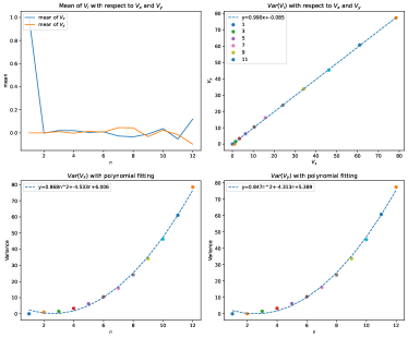
Figure 1: Variance and mean value of $V_{i}$ with respect to $V_{x}$ and $V_{y}$.

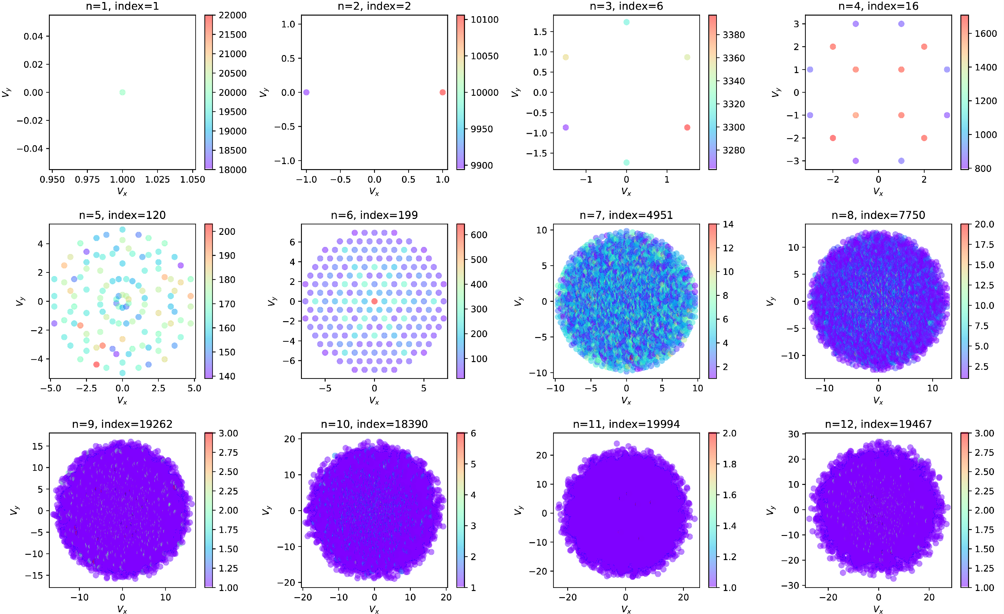
Figure 2: Visualization of random variables generation with n ranging from 1 to 12 in 20,000 simulations. Each point on the graph represents a possible random variable, with the color indicating the frequency of occurrence.

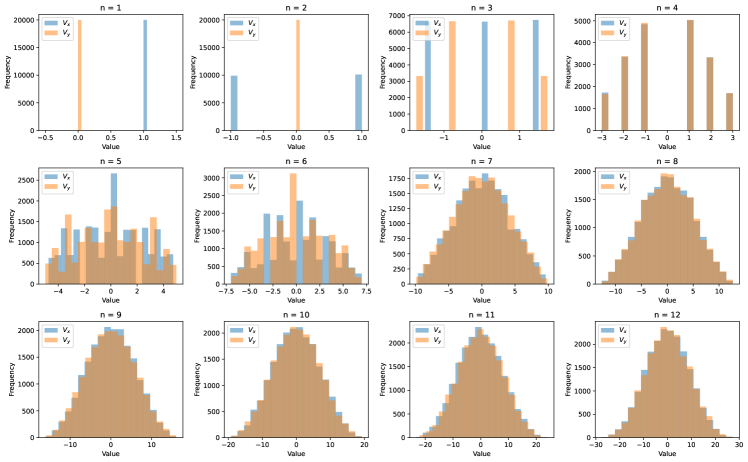
Figure 3: Histogram of random variables with respect to $V_{x}$ and $V_{y}$.

III.2 Simulating random variables for random walk

One common way to simulate random walk is adding a sequence of i.i.d. random variables. For example $\vec{V_{i}}$ form a normal distribution $N(\mu,\sigma^{2})$, where $\mu$ and $\sigma$ are the mean and standard deviations of the normal distribution, respectively. Then the sum of normally distributed random variables is a random walk (Lawler and Limic, 2010).

$$S_{t}=\sum_{i=0}^{t}\vec{V_{i}},$$ (14)

where $\vec{V_{i}}$ is marked as a step, $V_{0}$ is the starting value of the random walk, and $t$ is the number of steps. Inspired by such method, we tend to use such method with random variables simulated from RPST to generate random walk.

To generate a ideal random variable $\vec{V_{i}}$, we first should determine the length of the possible permutation sequence, i.e. $n$ in RVG.

Based on the maximum RPS entropy, an natural idea is to delve a distribution from RPST, and use it as probabilities associated with each possible permutation sequence. Given a fixed set $\Lambda=\left\{\lambda_{1},\lambda_{2},\dots,\lambda_{n}\right\}$, the belief assigned to possible permutation sequence whose cardinality is identical is the same. When the length of a possible permutation sequence is determined, then we can select one of the possible permutation sequence evenly as our probabilities association method, and that’s why we use uniform distribution as the probabilities associated with each possible permutation sequence in section III.1.

Definition 9.

(RPST distribution). Given a maximum length of permutation sequences $N$, there are $P(N,n)$ choices to select a possible permutation sequences with length of $n$, then the possibility of selecting $n$ as the length of possible permutation sequence combined with the maximum RPS entropy, is defined as RPST distribution.

$$P_{RPS}(n|N)=P(N,n)\cdot\mathcal{M}_{i=n,j}=\frac{P(N,n)[F(n)-1]}{\sum_{i=1}^{N}\left[P(N,i)(F(i)-1)\right]}.$$ (15)

To illustrate the the validity of the proposed method, we consider the following way to select a possible length $n$ for permutation sequence with the same probability:

Definition 10.

(Permutation distribution). Given a maximum length of permutation sequences $N$, there are $\sum_{i=1}^{N}i!$ kinds of permutation sequences, the permutation distribution is defined to choose a possible length $n$ based on the number of permutation cases.

$$P_{Per}(n|N)=\frac{P(N,n)}{\sum_{i=1}^{N}P(N,n)}=\frac{P(N,n)}{F(N)-1}=\frac{P(N,n)}{\lfloor e\cdot N!\rfloor},$$ (16)

i.e., the possibility of selecting a possible sequence length $n$ is in proportion to the magnitude of permutation $P(N,n)$. When the In other words, given a maximum length of permutation sequences $N$, the probability of selecting a possible permutation sequence from all $\lfloor e\cdot n!\rfloor$ sequences is $1/(\lfloor e\cdot n!\rfloor)$.

	$N$	$n=N-5$	$n=N-4$	$n=N-3$	$n=N-2$	$n=N-1$	$n=N$	$\sum_{n=N-5}^{N}P(n|N)$
$P_{Per}(n|N)$	6	3.0700e-3	1.5340e-2	6.1350e-2	1.8405e-1	3.6810e-1	3.6810e-1	1.0000e-0
	10	3.0700e-3	1.5330e-2	6.1310e-2	1.8394e-1	3.6788e-1	3.6788e-1	9.9941e-1
	$\vdots$
	18	3.0700e-3	1.5330e-2	6.1310e-2	1.8394e-1	3.6788e-1	3.6788e-1	9.9941e-1
	$\vdots$
	$\infty$	$\frac{1}{5!e}$	$\frac{1}{4!e}$	$\frac{1}{3!e}$	$\frac{1}{2!e}$	$\frac{1}{e}$	$\frac{1}{e}$	$\frac{163}{60e}$
$P_{RPS}(n|N)$	6	0.0000e-0	7.0000e-5	1.0800e-3	1.3820e-2	1.4035e-1	8.4468e-1	1.0000e-0
	10	0.0000e-0	1.0000e-5	2.1000e-4	5.0200e-3	9.0430e-2	9.0433e-1	1.0000e-0
	$\vdots$
	18	0.0000e-0	0.0000e-0	3.0000e-5	1.5500e-3	5.2550e-2	9.4587e-1	1.0000e-0
	$\vdots$
	$\infty$	0	0	0	0	0	1	1

Table 1: The last $6$ elements’ probability assignment of distribution $P_{Per}(n|N)$ and $P_{RPS}(n|N)$, all results are rounded to $5$ digits.

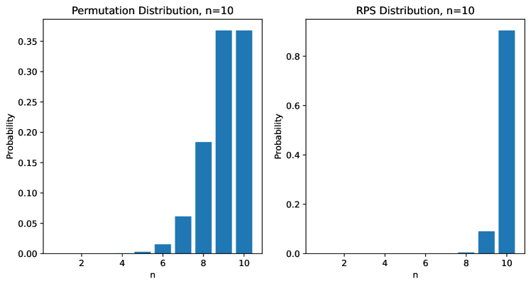
Figure 4: Discrete probability distribution of $P_{Per}(n|N)$ and $P_{RPS}(n|N)$ with $N=10$.

We plot the discrete probability distribution of $P_{Per}(n|N)$ and $P_{RPS}(n|N)$ with $N=10$ in fig. 4. And table 1 lists the details of the last $6$ elements’ probability assignment for those two distribution. Based on above, it is obvious that the last $6$ elements take up most of the probability assignment. Thus, when selecting a possible length for permutation sequences, $P_{Per}(n|N)$ tends to choice $n$ from $[N-5,N]$, while $P_{Per}(n|N)$ like to assign most of the probability to $n=N$ with a bigger $N$. The limit form of $P_{Per}(n|N)$ and $P_{RPS}(n|N)$ will be discussed in appendix A.

III.3 Generating random walk with random variables

Using section III.2 as a construction of generating random walk, we design the following algorithm to generate random walk with random variables.

Definition 11.

(Random Walk Generator, RWG). Given a positive integer $T$ denoted as time steps, the maximum length of permutation sequence $N$, and the distribution method $P(n|N)$, the random walk generator (RWG) is defined by Algorithm 2.

Result: A matrix $T_{t\times 2}$ representing the discrete time stochastic process.

Input: An integer $t$ indicating the number of time steps, a selection method $P$ ($P_{Per}(n|N)$ and $P_{RPS}(n|N)$), the maximum sequence length $N$.

Output: A matrix $T$ with size of $t\times 2$.

1 $Len_{S}et\leftarrow\textnormal{{GenLen}}(P,N)$

/* Create a set of lengths with constraints to maximum length of $N$, the set is used for generating random variables. */

2 for $i=2$ to $t$ do

3       $Temp\_Vec=\textnormal{{RVG}}(Len\_Set_{i-1})$ $T_{i}\leftarrow T_{i-1}+Temp\_Vec$

4      

5 end for

/* Generate value of random walk at each time step. */

6 return $T$

Algorithm 2 Random Walk Generator

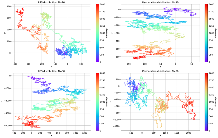
Figure 5: Visualization of random walk from distribution $P_{Per}(n|N)$ and $P_{RPS}(n|N)$, where color map is showing the time steps.

Algorithm 2 takes the number of time steps $t$, a distribution $P$ used for selection method, and $N$ indicating the maximum length of permutation sequence, as inputs, returning a matrix $T$ storing values at each time step.

Figure 5 shows results across different $N$ and $P$. The color map illustrates the temporal evolution of the random walk’s trajectory. As $N$ increases, the discrete-time stochastic process $T$, which is generated from RPST distribution $P_{RPS}$, shows a motion pattern resembling random walk, characterized by randomly distributed points in space.

Comparing the results of $N=10$ and $N=30$, the motion exhibits stochastic self-similarity as in random walk. This is because at each time step, this RPST-generated motion will walk through the space for each $n$ directions ($n$ being the possible length of permutation sequence with maximum length of $N$). These $n$ paths can be decomposed into $x$ and $y$ directions in perpendicular coordinates, similar to the two-dimensional random walk where the walker randomly chooses one of two perpendicular directions with a fixed step size.

To compare the proposed method’s limit scale form with the Wiener process, we employ a method similar to definition 7, to simulate the limit scale form of the RPST-generated random walk.

$$RW_{n,N}(t)=\frac{\sqrt{\varrho}}{N\sqrt{N}}\frac{1}{\sqrt{n}}\sum_{1\leq i\leq\lfloor nt\rfloor}\vec{V_{i}},t\in[0,1],$$ (17)

where $N$ is the maximum length of a permutation sequence, $n$ is the number of time step, and $\varrho$ is a variance control factor that scales the variance of RPST-generated random walk . As $N,n\to infty$, $RW_{n,N}(t)$ toward to a Wiener process, the details will be discussed in appendix A.

The only difference to Wiener process as a limit scale form of random walk, is that the re-scaling factor $\sqrt{\varrho}/({N\sqrt{N})}$. this is due to the fact that the random variables generated from RPST have variance growing like binomial function, as shown in fig. 1. So this redesigned re-scaling factor ensures the variance of random variables is invariant to $n$.

Since simulations on computers are actually discrete, and for convenience of illustration, we generate the proposed stochastic process $T$ with time step of $2,000$, and re-scale to $RW_{n,N}(t)$ with setting $\varrho=24$.

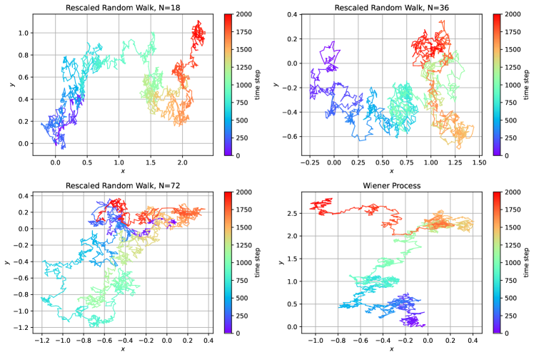
Figure 6: Scaled Random walk with different $N$ and Wiener process with time steps $2,000$ and variance control factor $\varrho=24$.

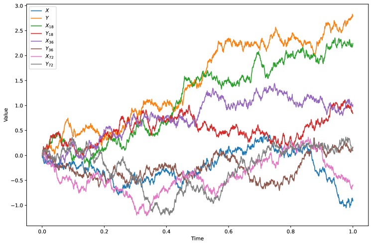
Figure 7: Component value of random walk and Wiener process of fig. 6, the $2,000$ time steps are converted to time $t\in[0,1]$ for convenience and $\varrho$ is set to 24 $\varrho=24$.

As shown in fig. 6, the scaling RPST-generated random walk do visually seem the same as standard Wiener process, not only the randomly walked point path, but also the boundaries. And more details about the component values about $X$ and $Y$ axis are plotted in fig. 7. Based on this result, it seems that the proposed stochastic process converges to Wiener process as $N$ increases. However, additional verification is required before reaching a definitive conclusion.

In fig. 8, the mean and variance values of various stochastic processes are compared to the Wiener process across different $\varrho$ values, with time steps and sample processes limited to $100$ and $200$, respectively. And the $5$ interval are set to $[0,20)$, $[0,40)$, $[0,60)$, $[0,80)$, $[0,100)$ to minimize errors.

Results show that all proposed methods with different $N$ exhibit properties similar to the Wiener process in terms of mean value and variance, where the mean value is zero and variance scales with time steps. Compared the sub-figures in fig. 8, the difference lies in the slope of variance, which is why we introduce the variance control factor $\varrho$ to regulate the variance of the proposed stochastic process. This ensures that the variance of the process aligns with that of a Wiener process.

From the results and analysis presented above, it is evident that as the sample size ($N$) increases, the RPST-generated random walk converges to a Wiener process, which is the limit scale form of a two-dimensional random walk. This demonstrates the successful derivation of a random walk from RPST.

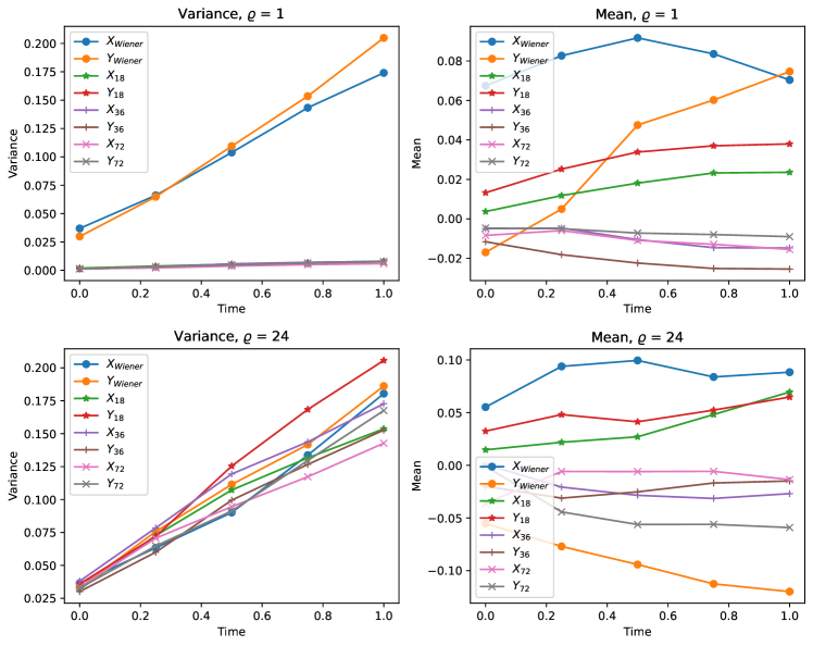
Figure 8: Variance (left) and mean (right) value of Wiener process $W(t)$ and limit scale form of random walk from RPST $RW_{n,N}(t)$ across various $N$ and variance control factor, time steps and number of simulations are set to $100,200$, respectively.

IV Conclusion

Random permutation set theory (RPST) is a promising extension of evidence theory that introduces ordered information to its reasoning framework. The indexed order in RPST can be viewed as a time series, which motivates the exploration of a connection between RPST and random walk, a fundamental topic in probability theory. This paper demonstrates that RPST can be used to construct a Gaussian random walk and, in the limit, a Wiener process. The established link between RPST and random walk provides insights into the physical meaning of RPST and enables its application in existing random walk domains. This not only expands the application scope of RPST but also provides insights for combination the strengths of both RPST and random walk for problem-solving.

Future investigations should concentrate on overcoming the limitations of current study. This may involve elucidating the physical implications of RPST through its association with random walks. Subsequently, the application of this random walk model to real-world scenarios, such as epidemiological modeling, financial market analysis and machine learning algorithm, could be explored.

AUTHOR DECLARATIONS

Conflict of Interest

The authors have no conflicts to disclose.

CRediT authorship contribution statement

Jiefeng Zhou: Conceptualization, Methodology, Formal analysis, Investigation, Writing-original draft, Writing-review & editing. Zhen Li: Validation. Yong Deng: Writing-review & editing, Supervision, Project administration, Funding acquisition.

Data Availability

The data that support findings of this study are available from the corresponding author upon reasonable request.

Appendix A Proof of deriving random walk from RPST

In this section, we will analyze the RPST-generated random walk in detail and demonstrate its similarities with random walk in mathematics.

A.1 Analysis on random variables

In section III, the random variables are first defined for generating random walk. these variables are generated using the order property of RPST. As a simulation method, its important statistic properties like expected value and variance should be reviewed.

A.1.1 Expected value analysis

Lemma 1.

(Expected value of a random variable). The expected value of a random variable generated with RVG is zero, namely,

$$\mathbb{E}\left[V_{i}\right]=0.$$ (18)

Proof.

As described in algorithm 1, when dealing with an integer set of length $N$, the likelihood of selecting a specific permutation sequence is equal, with a probability of

$$P\left\{V=V_{i}\right\}=\frac{1}{N!}.$$ (19)

To determine the expected value in each direction, we calculate the frequency of numbers appearing in a fixed direction, such as $\frac{2\pi\cdot i}{N}$. The magnitude of this direction in a simulation is determined by

$$|V_{component}|=P\left\{V=V_{i}\right\}\cdot\sum_{j=1}^{N}\left[j\cdot\left(N-1\right)!\right]=\frac{1+N}{2}.$$ (20)

Due to symmetry in direction generation and identical magnitudes, the resultant sum vector $\left(V_{x},V_{y}\right)$ is anticipated to yield a value of $0$. Thus, the expected value of $\left(V_{x},V_{y}\right)$ or $V_{i}$ is

$$\mathbb{E}\left[\left(V_{x},V_{y}\right)\right]=\mathbb{E}\left[V_{i}\right]=0$$ (21)

∎

fig. 1 also displays the mean value of $V_{x},V_{y}$ in $20,000$ simulations, suggesting the expected value of $\vec{V_{i}}$ is zero.

A.1.2 Variance analysis

Variance is a measure of dispersion, which is pretty useful in generating random walk. As shown in fig. 1, the variance of $V_{x}$ and $V_{y}$ are quantitatively identical, and both of them exhibit a binomial growth rate with respect to $N$.

Lemma 2.

(Variance of a random variable). The variance of a random variable generated from RVG is a binomial function on $N$, namely:

$$Var(\vec{V_{i}})\propto(N^{2}+N).$$ (22)

Proof.

In fig. 1, it can be directly observed that the variance of both $V_{x}$ and $V_{y}$ is in proportion to $N^{2}$. And this relationship can be explained from the following perspectives.

As indicated in section A.1.1, the expected value of magnitude in each direction is proportional to the maximum length of permutation sequence $N$, while the expected value of $\vec{V_{i}}$ remains zero, as demonstrated in lemma 1. This ensures that as $N$ increases, the distribution of random variables maintains its symmetry, resembling a round boundary. The size of this boundary is determined by the value of $N$, as shown in fig. 2. Therefore, there exists a critical value $N_{0}$, such that when $N_{2}>N_{1}\geq N_{0}$, random variables $\vec{V_{i}}_{2}$ generated with $N=N_{2}$ can be represented by the random variables $\vec{V_{i}}_{1}$ generated with $N=N_{1}$, denoted as

$$\vec{V_{i}}_{2}=f(N_{2}-N_{1})\cdot\vec{V_{i}}_{1},$$ (23)

where $f(x)$ is a function $\mathbb{R}\to\mathbb{R}$, as shown in section A.1.1.

Then based on the propagation property of variance:

$$Var(aV)=a^{2}Var(V),$$ (24)

where $a$ is a constant, and section A.1.2, one can easily delve such result in lemma 2. ∎

A.2 Analysis on permutation distribution and RPST distribution

Lemma 3.

(Limit form of RPST distribution). When $N\to infty$, the RPST distribution will converge to the following form:

$$\lim_{N\to\infty}P_{RPS}(n=N|N)=1$$ (25)

Proof.

The RPST distribution is based on the maximum RPS entropy, this distribution will surely converge to $P(n=N|N)=1$, as suggested in table 1. This result is determined by its definition on eq. 15. In our previous work (Zhou et al., 2024), we proved that

$$\lim_{N\to\infty}\sum_{i=1}^{N}\left[P(N,i)\left(F(i)-1\right)\right]-e\cdot(N!)^{2}=0,$$ (26)

$$F(N)-1=\lfloor e\cdot N!\rfloor-1$$ (27)

Compared with $P(N,n)[F(n)-1]$, we get

$$\lim_{N\to\infty}P_{RPS}(n=N|N) =\frac{N!\left(\lfloor e\cdot N!\rfloor-1\right)}{e(N!)^{2}}$$

$$=\lim_{N\to\infty}\frac{N!\lfloor e\cdot N!\rfloor}{e(N!)^{2}}-\lim_{N\to\infty}\frac{1}{e(N!)^{2}}$$

$$=1-0$$

$$=1$$ (28)

This result ensures that when $N$ is bigger enough, this distribution will converge to the following probability distribution:

$$P_{RPS}(n|N)=\begin{cases}1,&n=N;\\ 0,&others.\end{cases}$$ (29)

∎

This probability distribution can be explained by the maximum entropy principle. This principle states that the distribution with the highest entropy is the most likely to represent the current state of a system. Therefore, the larger the value of $N$, the more likely it is that the system will choose the permutation sequence with the maximum length. This is because a longer permutation sequence indicates more uncertainty.

However, the probability assignment in Permutation distribution will not converge to a single element. Conducted from eq. 16, we have

$$\lim_{N\to\infty}P_{Per}(n|N) =\lim_{N\to\infty}\frac{P(N,n)}{\lfloor e\cdot N!\rfloor}$$

$$=\lim_{N\to\infty}\frac{N!}{(N-n)!}/\left(\lfloor e\cdot N!\rfloor\right)$$

$$=\lim_{N\to\infty}\frac{1}{e(N-n)!}.$$ (30)

Thus, permutation distribution will converge to the limit form as shown in table 1. In contrast to the RPST distribution, the permutation distribution exhibits a greater degree of variability, which hinders the generation of i.i.d. random variables. Consequently, it is not suitable for simulating random walks.

A.3 Analysis on RPST-generated random walk

In previous section, it is proved that RPST distribution will converge to a probability distribution shown in eq. 29, ensuring its generation of i.i.d. random variables, which is a necessity for generating random walk. And some statistics properties of RPST-generated random walk are analysed in this section.

The histogram in fig. 3 displays the generation of random variables. It is expected that, for a fixed value of $N$, the RVG will produce random vectors that adhere to a normal distribution. This convergence towards a normal distribution is controlled by the central limit theorem (CLT) and Donsker’s theorem, which ensure that as $N\to\infty$, the summation vector $\vec{V_{i}}=(V_{x},V_{y})$ will be distributed according to a normal distribution $N(0,\sigma^{2}_{N})$, where $\sigma^{2}_{N}=f(N)\sigma^{2}$ and $f(N)\propto N^{2}$ is a binomial function with respect to $N$. This result is supported by lemma 2 and fig. 1.

Due to the binomial growth of variance, we design the re-scaling factor $\sqrt{\varrho}/(N\sqrt{N})$ to fitting the variance pattern of Wiener process. This re-scaling factor comes from the following theorem:

Theorem 1.

The RPST-generated random walk $RW(t)$ can be converted to Wiener process if the following limit form exists:

$$W(t)=\lim_{n,N\to\infty}RW_{n,N}(t)=\lim_{n,N\to\infty}\frac{\sqrt{\varrho}}{N\sqrt{N}}\frac{1}{\sqrt{n}}\sum_{1\leq i\leq\lfloor nt\rfloor}\vec{V_{i}},t\in[0,1].$$ (31)

Proof.

The difference between $RW(t)$ and Gaussian random walk lies in the variance, if we can scale the variance of $RW(t)$ to fit into normal distribution, then following definition 7 one can easily proves it.

As demonstrated in lemma 1 and lemma 2, we get

$$\mathbb{E}\left[RW(t)\right]=\mathbb{E}\left[\sum_{i=0}^{t}V_{i}\right]=0.$$ (32)

Then we have

$$\mathbb{E}\left[RW^{2}(t)\right]=\sum_{i=1}^{t}\mathbb{E}\left[V_{i}^{2}\right]+2\sum_{1\leq i<j<t}\mathbb{E}\left[V_{i}V_{j}\right].$$ (33)

Since random variables are independent with each other, then for any $i\neq j$, $\mathbb{E}\left[V_{i}V_{j}\right]=0$.

Using the equation of variance

$$Var(X)=\mathbb{E}\left[X^{2}\right]-\mathbb{E}\left[X\right]^{2},$$ (34)

we get

$$\mathbb{E}\left[V_{i}^{2}\right]=Var(V_{i})\propto(N^{2}+N).$$ (35)

Together with section A.3, we get

$$\mathbb{E}\left[RW^{2}(t)\right]=\sum_{i=1}^{t}\mathbb{E}\left[V_{i}^{2}\right]=t\cdot\left(Var(V_{i})\right)\propto t(N^{2}+N).$$ (36)

Finally, the variance of $RW(t)$ has the following property

$$Var(RW(t))=\mathbb{E}\left[RW^{2}(t)\right]\propto t(N^{2}+N).$$ (37)

Compared with Gaussian random walk, the growing speed of $Var(RW(t))$ is additionally multiplied by $N^{2}+N$. In other words, after $t-s$ steps, the increments of Gaussian random walk $Z_{t-s}\sim N(0,(t-s)\sigma^{2})$, while in random walk from RPST we have $Z_{t-s}\sim N(0,(t-s)(N^{2}+N)\sigma^{2})$. Thus, based on the propagation property of variance, we construct $V_{i}^{\prime}=V_{i}/{N\sqrt{N}}$ to offset the term $(N^{2}+N)$. But there still exists a coefficient between the scaling $V_{i}$ and the step of Gaussian random walk (or Wiener process in limiting form), as shown in fig. 8, so we design a variance control factor $\varrho$, then the final scaling factor would be $\sqrt{\varrho}/({N\sqrt{N}})$. We set $\varrho=24$ to approximating Gaussian random walk.

So after scaling the RPST-generated random walk to Gaussian random walk, one can use Donsker’s theorem and definition 7 to construct the form in theorem 1 to convert a RPST-generated random walk to a Wiener process, thus theorem 1 is proved.

∎

Similar to Wiener process, the limit scale form of random walk from RPST $RW_{n,N}(0)$ is also characterised by the following properties:

• $RW_{n,N}(0)=0$. This prosperity is achieved by setting the starting point to zero $V_{0}=0$.

• $RW_{n,N}(t)$ has independent increments. This property is determined by the fact that each random variables are independent with each other, following a step size distribution of normal distribution $N(0,f(N)\sigma^{2})$.

• For any $0\leq s<t$, the increments $RW_{n,N}(t)-RW_{n,N}(s)\sim N(0,t-s)$. This can be done by setting the variance factor $\varrho=24$, as shown in fig. 8.

• $RW_{n,N}(t)$ is almost surely continuous in $t$, this is ensured by Donsker’s theorem as $N,n\to\infty$.

References

- Ansari-Rad, Abdi, and Arzi (2012) Ansari-Rad, M., Abdi, Y., and Arzi, E., “Monte Carlo random walk simulation of electron transport in dye-sensitized nanocrystalline solar cells: Influence of morphology and trap distribution,” The Journal of Physical Chemistry C 116, 3212–3218 (2012).
- AP (1967) AP, D., “Upper and lower probabilities induced by a multivalued mapping,” The Annals of Mathematical Statistics 38, 325–339 (1967).
- Chen and Deng (2023) Chen, L. and Deng, Y., “Entropy of Random Permutation Set,” Communications in Statistics - Theory and Methods , 1–19 (2023).
- Chen, Deng, and Cheong (2023a) Chen, L., Deng, Y., and Cheong, K. H., “The Distance of Random Permutation Set,” Information Sciences 628, 226–239 (2023a).
- Chen, Deng, and Cheong (2023b) Chen, L., Deng, Y., and Cheong, K. H., “Permutation Jensen–Shannon divergence for Random Permutation Set,” Engineering Applications of Artificial Intelligence 119, 105701 (2023b).
- Contreras-Reyes and Kharazmi (2023) Contreras-Reyes, J. E. and Kharazmi, O., “Belief fisher–shannon information plane: Properties, extensions, and applications to time series analysis,” Chaos, Solitons & Fractals 177, 114271 (2023).
- Cui et al. (2022) Cui, H., Zhou, L., Li, Y., and Kang, B., “Belief entropy-of-entropy and its application in the cardiac interbeat interval time series analysis,” Chaos, Solitons & Fractals 155, 111736 (2022).
- Deng and Deng (2022) Deng, J. and Deng, Y., “Maximum entropy of random permutation set,” Soft Computing 26, 11265–11275 (2022).
- Deng (2016) Deng, Y., “Deng entropy,” Chaos, Solitons & Fractals 91, 549–553 (2016).
- Deng (2022) Deng, Y., “Random Permutation Set,” INTERNATIONAL JOURNAL OF COMPUTERS COMMUNICATIONS & CONTROL 17 (2022), 10.15837/ijccc.2022.1.4542.
- Einstein (1956) Einstein, A., Investigations on the Theory of the Brownian Movement (Courier Corporation, 1956).
- Gao et al. (2023) Gao, L., Yin, M., Xiao, F., and Cao, Z., “A complex belief jensen-shannon divergence in complex evidence theory for decision-making,” in 2023 IEEE International Conference on Unmanned Systems (ICUS) (IEEE, 2023) pp. 299–304.
- Kang and Deng (2019) Kang, B. and Deng, Y., “The maximum deng entropy,” IEEE Access 7, 120758–120765 (2019).
- Kessing et al. (2022) Kessing, R. K., Yang, P.-Y., Manmana, S. R., and Cao, J., “Long-Range Non-Equilibrium Coherent Tunneling Induced by Fractional Vibronic Resonances,” The Journal of Physical Chemistry Letters 13, 6831–6838 (2022), arxiv:2111.06137 [cond-mat, physics:physics, physics:quant-ph] .
- Kharazmi and Contreras-Reyes (2023) Kharazmi, O. and Contreras-Reyes, J. E., “Deng–Fisher information measure and its extensions: Application to conway’s game of life,” Chaos, Solitons & Fractals 174, 113871 (2023).
- Lawler and Limic (2010) Lawler, G. F. and Limic, V., Random walk: a modern introduction, Vol. 123 (Cambridge University Press, 2010).
- Li and Xiao (2023) Li, S. and Xiao, F., “Normal distribution based on maximum deng entropy,” Chaos, Solitons & Fractals 167, 113057 (2023).
- Liu et al. (2024) Liu, R., Zhan, T., Li, Z., and Deng, Y., “Learnable wsn deployment of evidential collaborative sensing model,” arXiv preprint arXiv:2403.15728 (2024).
- Liu, Zhao, and Xiao (2023) Liu, S., Zhao, Y., and Xiao, F., “A new complex deng entropy with its application in pattern classification,” in 2023 IEEE International Conference on Unmanned Systems (ICUS) (IEEE, 2023) pp. 1310–1315.
- Ortiz-Vilchis, Lei, and Ramirez-Arellano (2024) Ortiz-Vilchis, P., Lei, M., and Ramirez-Arellano, A., “Reformulation of deng information dimension of complex networks based on a sigmoid asymptote,” Chaos, Solitons & Fractals 180, 114569 (2024).
- Shafer (1976) Shafer, G., A Mathematical Theory of Evidence, Vol. 42 (Princeton university press, 1976).
- Shannon (1948) Shannon, C. E., “A mathematical theory of communication,” The Bell system technical journal 27, 379–423 (1948).
- Thompson, Kienle, and Schwartz (2022) Thompson, C. J., Kienle, D. F., and Schwartz, D. K., “Enhanced Facilitated Diffusion of Membrane-Associating Proteins under Symmetric Confinement,” The Journal of Physical Chemistry Letters 13, 2901–2907 (2022).
- Tojo and Argyrakis (1996) Tojo, C. and Argyrakis, P., “Correlated random walk in continuous space,” Physical Review E 54, 58 (1996).
- Wang et al. (2021) Wang, Y., Cao, X., Weng, T., Yang, H., and Gu, C., “A convex principle of search time for a multi-biased random walk on complex networks,” Chaos, Solitons & Fractals 147, 110990 (2021).
- Yang and Xiao (2024) Yang, X. and Xiao, F., “A novel uncertainty modeling method in complex evidence theory for decision making,” Engineering Applications of Artificial Intelligence 133, 108164 (2024).
- Zeng and Xiao (2023) Zeng, Z. and Xiao, F., “A new complex belief entropy of 2 divergence with its application in cardiac interbeat interval time series analysis,” Chaos, Solitons & Fractals 172, 113542 (2023).
- Zhan, Li, and Deng (2024) Zhan, T., Li, Z., and Deng, Y., “Random Graph Set and Evidence Pattern Reasoning Model,” (2024), arxiv:2402.13058 [cs] .
- Zhang, Li, and Deng (2018) Zhang, Q., Li, M., and Deng, Y., “Measure the structure similarity of nodes in complex networks based on relative entropy,” Physica A: Statistical Mechanics and its Applications 491, 749–763 (2018).
- Zhao, Li, and Deng (2023) Zhao, T., Li, Z., and Deng, Y., “Information fractal dimension of Random Permutation Set,” Chaos, Solitons & Fractals 174, 113883 (2023).
- Zhao, Li, and Deng (2024) Zhao, T., Li, Z., and Deng, Y., “Linearity in deng entropy,” Chaos, Solitons & Fractals 178, 114388 (2024).
- Zhou et al. (2024) Zhou, J., Li, Z., Cheong, K. H., and Deng, Y., “Limit of the maximum random permutation set entropy,” arXiv preprint arXiv:2403.06206 (2024).
- Zhou et al. (2022) Zhou, Q., Cui, Y., Li, Z., and Deng, Y., “Marginalization in random permutation set theory: From the cooperative game perspective,” Nonlinear Dynamics , 10.1007/s11071–023–08506–7 (2022).