EC 19529–4430: SALT identifies the most carbon- and metal-poor extreme helium star

Abstract

 EC 19529$-$4430 was identified as a helium-rich star in the Edinburgh-Cape Survey of faint-blue objects and subsequently resolved as a metal-poor extreme helium (EHe) star in the SALT survey of chemically-peculiar hot subdwarfs. This paper presents a fine analysis of the SALT high-resolution spectrum.  EC 19529$-$4430 has $T_{\rm eff}=20\,700\pm 250$ K, $\log g/{\rm cm\,s^{-2}}=3.49\pm 0.03$, and an overall metallicity some 1.3 dex below solar; surface hydrogen is $\approx 0.5\%$ by number. The surface CNO ratio 1:100:8 implies that the surface consists principally of CNO-processed helium and makes  EC 19529$-$4430 the coolest known carbon-poor and nitrogen-rich EHe star. Metal-rich analogues include V652 Her and  GALEX J184559.8$-$413827. Kinematically, its retrograde orbit indicates membership of the galactic halo. No pulsations were detected in TESS photometry and there is no evidence for a binary companion.  EC 19529$-$4430 most likely formed from the merging of two helium white dwarfs, which themselves formed as a binary system some 11 Gyr ago.

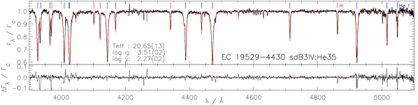
Figure 1: The RSS spectrum of  EC 19529$-$4430 (black) with the best-fit model (red) having $T_{\rm eff}=20\,650\pm 130$ K, $\log g/{\rm cm\,s^{-2}}=3.51\pm 0.02$, and $n_{\rm H}=0.0053\pm 0.0002$ ($\log y=2.27\pm 0.02$) (formal errors). The lower panel shows the residuals. Hydrogen Balmer and neutral helium absorption lines are marked in red and blue, respectively.

1 Introduction

Extreme helium stars (EHes) are characterised by their spectral types A and B, weakness or absence of hydrogen Balmer lines, and strength of neutral helium lines. Being rare and luminous, their lifetimes must be short, and yet they are located in all major components of the galaxy (Philip Monai et al., 2023). High carbon and/or nitrogen abundances indicate evolved surfaces revealed through a catastrophic event in their history, generally thought to be the merger of two white dwarfs (Saio & Jeffery, 2000, 2002). Their surface composition and distribution suggest a connection with other hydrogen-deficient stars including the cooler R Coronae Borealis variables (RCB) (Jeffery, 1994), dustless hydrogen-deficient carbon stars (dlHdC) (Warner, 1967; Crawford et al., 2023; Tisserand et al., 2023) and the hotter hydrogen-deficient hot subdwarfs (Hesd) (Saio & Jeffery, 2000; Zhang & Jeffery, 2012) and O(He) stars (Reindl et al., 2014).

Following a spectroscopic survey of luminous blue stars (Drilling, 1980, 1983), the number of confirmed EHes remained at roughly 17 from the early 1980s until the commencement of the Southern African Large Telescope (SALT) survey of chemically-peculiar hot subdwarfs in 2016 (Jeffery et al., 2021) (SALT1 hereafter). The Edinburgh-Cape (EC) survey of faint blue stars (Stobie et al., 1997; Kilkenny et al., 1997; O’Donoghue et al., 2013; Kilkenny et al., 2015; Kilkenny et al., 2016) classified a number of stars as He-sdB, a classification which overlaps the sdOD stars identified by Green et al. (1986) and the EHe stars as discussed by Drilling et al. (2013). SALT1 observations of He-sdB stars from the EC and other surveys revealed 3 new low-gravity B-type EHe stars, namely  GALEX J184559.8$-$413827(=J1846$-$4138),  EC 19529$-$4430, and EC 20236–5703 (Jeffery, 2017; Jeffery et al., 2021). Concurrently, the Tisserand et al. (2022) survey of dustless hydrogen-deficient carbon stars identified 2 new A-type EHes, namely A208 (J182447.94–221429.1) and A798 (J183357.03+052917.0). Meanwhile, several helium-rich subdwarfs were recognised to have properties similar to the hot high-gravity EHe star LS IV$+6^{\circ}2$ (Jeffery, 1998) including PG 1415+492 (Ahmad & Jeffery, 2003) and PG 0135+243 (Moehler et al., 1990). Stars such as BPS CS 22940–0009 (Snowdon et al., 2022), EC 20187–4939 (Scott et al., 2023), and others (Naslim et al., 2010), suggest that a continuous sequence extends to the helium-rich sdO stars.

A preliminary analysis of  EC 19529$-$4430 ($\alpha_{2000}=19{\rm h}\,56{\rm m}\,30.7{\rm s}$, $\delta_{2000}=-44^{\circ}\,22\arcmin\,19\arcsec$, showed it to be the coolest star in SALT1. At low-resolution, the spectrum “shows no ionized helium lines (including Heii 4686 Å) and Balmer lines much weaker than the neutral helium lines. A defining feature is the weakness of all metal lines and the narrow wings of the H and He I lines” (Jeffery et al., 2021). Philip Monai et al. (2023) found  EC 19529$-$4430 to be a halo object in a retrograde orbit. The weak metal-lined spectrum and low surface gravity demands a more careful analysis with model atmospheres of appropriate composition and regard to possible departures from LTE. The likely age and retrograde orbit deserve further discussion in terms of origin and evolution.

The observations on which this analysis is based are described in § 2. The model atmospheres underlying the analysis are described in § 3. The spectral analysis itself is presented in § 4. § 5 discusses the distance and kinematics. § 6 discusses the overall properties and evolutionary status and concludes the paper.

Table 1: Radial velocities measured from blue HRS spectra of  EC 19529$-$4430. “RSS” shows the measurement reported in SALT1. Radial velocities for individual observations are measured in two wavelength ranges relative to an average spectrum. “Mean” shows the averages and standard deviations. “Template” shows the velocities of the average spectrum relative to a model, and the bottom line indicates the adopted barycentric mean velocity.

Date	Run	JD	$\sigma_{4540}$	$\delta V$(4500-4700Å)	$\delta V$(4300-4500Å)
				$\mbox{km}\,\mbox{s}^{-1}$	$\mbox{km}\,\mbox{s}^{-1}$
20180516	RSS			$5\pm 3$ (SALT1)
20190323	H0049	2458566.631215	0.010	$0.290\pm 0.035$	$-0.531\pm 0.301$
20190329	H0021	2458572.619016	0.009	$-0.117\pm 0.032$	$-0.234\pm 0.315$
20190329	H0022	2458572.631412	0.011	$-0.151\pm 0.047$	$-0.200\pm 0.353$
20210801	H0015	2459428.269282	0.030	$-1.863\pm 0.115$	$-0.320\pm 0.116$
20210823	H0025	2459450.464167	0.058	$0.889\pm 0.057$	$0.467\pm 0.112$
20210825	H0018	2459452.458264	0.060	$0.696\pm 0.099$	$2.120\pm 0.196$
20210829	H0017	2459456.446146	0.051	$-0.913\pm 0.254$	$-0.601\pm 0.172$
	Mean			$-0.17\pm 0.96$	$0.10\pm 0.96$
	Template		0.006	$+9.73\pm 0.57$	$+11.38\pm 1.02$
				$10.32\pm 0.70$

2 Observations

Observations were obtained in 2019 March and April with SALT using both the High Resolution Spectrograph (HRS) and the Robert Stobie Spectrograph (RSS). These are described in Section 2 and Appendix A of SALT1. The methods used for data reduction are described in SALT1 (RSS) and by Snowdon et al. (2022) (HRS). Additional short exposure HRS observations were obtained during 2021 August and September in order to establish radial-velocity behaviour. For these and for all the red-arm HRS observations we have used the SALT pipeline reductions as described by Kniazev (2016).

The RSS spectrum and a model fit is shown in Fig. E.1 of SALT1. Fig. 1 shows the same spectrum together with a revised model solution which will be discussed below. The He i absorption lines are readily apparent and everywhere narrower than in helium-rich hot subdwarfs, but less sharp than in the lowest-gravity extreme helium stars. The Balmer lines are stronger than in most EHe stars, but similar in strength to those seen in J1846$-$4138 (Jeffery, 2017). There are no detectable Heii lines in the RSS spectrum. The spectrum bears similarities to EHe star V652 Her (Jeffery et al., 2001, 2015), including in particular the extremely rich spectrum of singly-ionized nitrogen (Fig. 1).

The wavelength range covered by the HRS spectrum is 3860 – 5519 Å  and has a S/N ratio in the range 140 – 200 at a resolution of $\approx 37,000$. The orders were rectified, mapped onto a common logarithmically spaced wavelength grid, and merged. The observed spectrum was further renormalised using appropriate models to guide the location of the local continuum in regions where strong lines overlap and to facilitate the measurement of abundances from narrow and weak lines.

Equivalent widths were measured for a substantial list of lines anticipated in early-type stellar spectra. For each predicted line, a region of spectrum is displayed and nearby continuum regions are identified manually. The upper and lower limits of the line itself are then identified, and the area of the line under the continuum is integrated and converted to an equivalent width ($W_{\lambda}$) The error is estimated from the variance of data in the local continuum, as described by Snowdon et al. (2022). Measurements used in subsequent analyses are shown in Appendix B.

Radial velocities of  EC 19529$-$4430 were measured from the HRS spectra as follows and are reported in Table 1. The signal-to-noise ratio of each spectrum is represented by $\sigma_{4540}$, the variance around the mean continuum between 4531 and 4548Å. A mean spectrum was formed from the sum of the first three HRS observations. Velocities were measured by cross-correlation relative to this mean spectrum in two wavelength ranges, namely 4300–4500Å which includes several broad Hei lines and 4500–4700Å which contains only sharp lines. Barycentric velocity corrections were applied prior to analysis. The heliocentric radial velocity of the mean spectrum was measured relative to a laboratory template (“Template” in Table 1).

With a standard deviation $<1$ $\mbox{km}\,\mbox{s}^{-1}$ over 7 observations on timescales of hours, days, weeks and years, there is no evidence for variability that would indicate membership of a close binary or of surface pulsations (“Mean” in Table 1). The mean HRS velocity is close enough to the RSS velocity to be unremarkable.

Photometric observations were obtained by the TESS spacecraft during cycles 13 and 27. These show no periodic variation at any frequency between 0.2 and 50 d^-1 with an amplitude $>0.02\%$ (4$\sigma$) of the mean flux. Pulsations are not expected for low-metallicity extreme helium stars with the properties of  EC 19529$-$4430, where sufficient iron is necessary to drive pulsations (Jeffery & Saio, 1999).

3 Model Atmospheres and Spectrum Synthesis

Analyses of astronomical spectra require the use of theoretical models adjusted to match the observations. In the present case we consider the spectrum to be formed in the atmosphere of a star which is in hydrostatic and radiative equilibrium. Other physics assumptions are implicit in the choice of computer code used to construct the models; for these we refer below to papers associated with the codes adopted.

Most of our models are computed with the codes sterne and spectrum described by Behara & Jeffery (2006) and Jeffery et al. (2001). These assume local thermodynamic equilibrium (LTE) for the atomic level populations, but depart from strict LTE in that they include electron scattering in the radiative transfer calculation for the source function. Bound-free opacities are included using data from the Opacity and Iron Projects (Seaton et al., 1994; Hummer et al., 1993). Line opacities due to 559316 lines (Kurucz & Bell, 1995) are also included. Pressure broadening in the H, Hei and Heii lines is treated using the tables of Vidal et al. (1973), Beauchamp et al. (1997) and Schöning & Butler (1989), respectively. At low densities, the Beauchamp et al. (1997) tables are supplemented by Voigt profiles using Stark broadening coefficients from Dimitrijevic & Sahal-Brechot (1984, 1990). Behara & Jeffery (2006) and Kupfer et al. (2017) compared models computed with sterne and atlas9 and atlas12 (Kurucz, 1993, 1996) respectively. They found differences of up to 2–3% in the line forming region, likely due to differences in the opacities and other model assumptions.

Analyses of the EHe stars V652 Her (Przybilla et al., 2005; Pandey & Lambert, 2017) and BD$+10^{\circ}2179$ (Pandey & Lambert, 2011; Kupfer et al., 2017) showed departures from LTE to be small except for very strong lines. In both analyses of V652 Her, the non-LTE hydrogen measurement was improved by almost eliminating line-to-line discrepancies, whilst the surface gravity measured from Hei lines was lower by $\sim 0.5$ dex than found previously (Hill et al., 1981; Lynas-Gray et al., 1984; Jeffery et al., 1999a, 2001). In contrast, the surface gravity measured by Kupfer et al. (2017) for BD$+10^{\circ}2179$ increased by $\sim 0.3$ dex relative to previous LTE and non-LTE analyses by Heber (1983); Pandey et al. (2006); Pandey & Lambert (2011). This is likely due to the adoption of an improved treatment of metal-line blanketing in the atlas12 model atmosphere and an improved model for the Hei atom in the line profile treatment.

On the basis of these previous studies, we have assumed for  EC 19529$-$4430 that departures from LTE will also be small except for very strong lines. However, since the strong lines affect the measurement of major parameters, our analysis included the effect of departures from LTE on the profiles of hydrogen and helium lines. First, we computed sterne equivalent models in LTE using version 208 of the code tlusty (Hubeny & Lanz, 1995, 2017a, 2017b, 2017c; Hubeny et al., 2021). These tlusty (LTE) models are consistent with the sterne (LTE) models, as established by comparing the temperature structures of the converged models (see § 4.3).

Using the structure of the previously converged LTE model, we used tlusty to solve the statistical equilibrium equations for H, Hei and Heii without computing any additional temperature corrections. Thus, we computed departure coefficients for the H, Hei and Heii ions with model atoms using 9, 24 and 20 energy levels respectively. These model ions, sourced from the tlusty website, used oscillator strengths and photoionisation cross sections from the Opacity Project database (Cunto et al., 1993), and level energies from NIST (Ralchenko & Kramida, 2020). Hence, using the formal solution code synspec version 54 (Hubeny & Lanz, 1995, 2017a, 2017b, 2017c; Hubeny et al., 2021), we computed grids of emergent spectra with these ions in non-LTE (synspec non-LTE). This approach mirrors that used by, for example, Przybilla et al. (2005) in their analysis of the extreme helium star V652 Her.

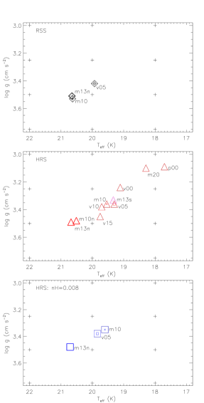
Figure 2: Solutions for $T_{\rm eff}$ and $\log g$ for  EC 19529$-$4430 for both RSS (top) and HRS spectra (middle). The bottom panel shows solutions for the HRS spectrum with $n_{\rm H}=0.008$. Labels m20, m10 (‘$\times$’) and p00 indicate fits using the second iteration sterne (LTE) $+$ spectrum (LTE) grid, with $\xi_{\rm turb}=0$ $\mbox{km}\,\mbox{s}^{-1}$. Labels v00, v05 (‘$\square$’), v10 and v15 indicate fits using the third iteration sterne (LTE) $+$ spectrum (LTE) grid (m13n10), with $\xi_{\rm turb}=0$, 5, 15 and 15  $\mbox{km}\,\mbox{s}^{-1}$. Heavy symbols indicate fits using the tlusty (LTE) $+$ synspec (non-LTE) grids m10n and m13n. The violet symbol, labelled m13s, refers to a fit using the tlusty (LTE) $+$ synspec (LTE) grid (m13n10), with $\xi_{\rm turb}=5$  $\mbox{km}\,\mbox{s}^{-1}$. Formal errors are shown for the RSS fits. Formal errors for the HRS fits are too small to show.

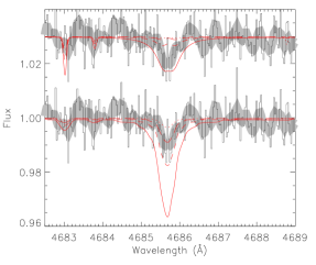
Figure 3: The HRS spectrum of  EC 19529$-$4430 (histogram) in the vicinity of Heii4686 compared with equivalent synspec (top) and sterne (bottom) models (red) having $T_{\rm eff}$ = 16 kK (dots), 18 kK (long dashes), 20 kK (short dashes) and 22 kK (solid). The thick grey curve shows the HRS spectrum smoothed with a 0.1Å FWHM Gaussian filter.

4 Stellar Atmosphere Analysis

4.1 Model atmosphere grids.

In the process of fine analysis, atmospheric parameters are obtained by finding a best-fit model spectrum, usually by interpolation in an appropriate grid. Typically, an estimate is made for the metal content and microturbulent velocity $\xi_{\rm turb}$, and then a grid of model atmospheres is computed to span a range of effective temperature $T_{\rm eff}$, surface gravity $g$ and hydrogen abundance $n_{\rm H}$ (fractional abundance by number). Since the composition and $\xi_{\rm turb}$ are not known ab initio, the process is iterative. The first (SALT1) iteration used solar metallicity grids (p00) (Jeffery et al., 2021), from which $T_{\rm eff}\approx 18\,500$K, $\log g/({\rm cm\,s^{-2}})\approx 3.4$ and $n_{\rm H}\approx 0.01$ was deduced. Alternatively, $\log y\equiv\log n_{\rm He}/n_{\rm H}\approx 2$. Predominantly weak metal lines suggested adoption of a metallicity scaled to 1/10 of the solar abundance (m10). $\xi_{\rm turb}=0$ $\mbox{km}\,\mbox{s}^{-1}$ was assumed. sterne models were calculated on grids defined by:
$T_{\rm eff}=16,18,20,22$ kK,
$\log g/({\rm cm\,s^{-2}})=2.50,2.75,3.00,3.25,3.50,3.75$, and
$n_{\rm H}=0.00,0.01,0.03$.
For completeness, model grids were also calculated with metallicity scaled to 1/100 (m20) and 1 times solar (p00).

The second iteration provided estimates of $T_{\rm eff}\approx 20\,000$K, $\log g/({\rm cm\,s^{-2}})\approx 3.5$ and $n_{\rm H}\approx 0.01$. From this, abundance estimates were obtained from measured equivalent widths, indicating an overall metallicity 1/20 times solar ($-1.3$ dex = m13), with the exception of nitrogen being close to $1\times$ solar (n10). New models were calculated on the same grid as above using this custom mixture (m13n10) and with $\xi_{\rm turb}=0$, 5, 10 and 15 $\mbox{km}\,\mbox{s}^{-1}$(abbreviated: v00, v05, v10 and v15). Abundances obtained from this third iteration were within 0.3 dex of those used as inputs, so the process was deemed to have converged.

LTE models were computed using tlusty on the same grids and mixtures as the sterne m10 and m13n10 grids. $\xi_{\rm turb}=5$ $\mbox{km}\,\mbox{s}^{-1}$ was adopted throughout. Departure coefficients were computed for hydrogen and helium, and hence model spectra were obtained with hydrogen and helium out of LTE. All other atoms were treated in LTE throughout. The resulting grids are labelled m10_nlte (or m10n) and m13n10_nlte (or m13n).

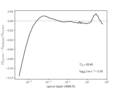
Figure 4: Comparison of temperature structures of tlusty and sterne model atmospheres in the sense $1-(T_{\rm STERNE}/T_{\rm TLUSTY})$ as a function of optical depth. Models are compared for $T_{\rm eff}=20\,000$ K, $\log g/({\rm cm\,s^{-2}})=3.5$, $n_{\rm H}=0.01$, $\xi_{\rm turb}=5$  $\mbox{km}\,\mbox{s}^{-1}$.

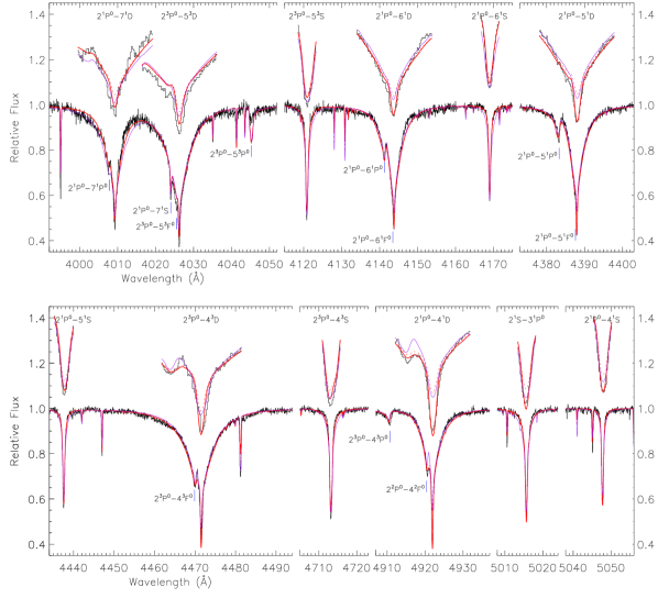
Figure 5: The HRS spectrum of  EC 19529$-$4430 in the vicinity of several Hei lines compared with the best-fit non-LTE model (bold red) and the best-fit LTE models computed with tlusty+synspec (dotted red) and sterne+spectrum (solid violet). The best-fit non-LTE model has $T_{\rm eff}=20\,680\pm 40$ K, $\log g/{\rm cm\,s^{-2}}=3.49\pm 0.01$, and $n_{\rm H}=0.0042\pm 0.0001$ ($\log y=2.37\pm 0.01$) (formal errors). Each Hei line is labelled by its transition. The cores of strong lines are duplicated above, with the wavelength scale expanded by a factor 5. Lines observed but not shown include $2^{3}P^{0}-4^{3}P^{0}$ 4517.4Å, $2^{1}S-4^{1}P^{0}$ 3964.7Å, $2^{1}P^{0}-8^{1}S$ 3935.9Å, and $2^{1}P^{0}-8^{1}D$ 3926.5Å.

4.2 Effective temperature and surface gravity.

We use the $\chi^{2}$ minimizer sfit (Jeffery et al., 2001) to optimise for $T_{\rm eff}$, $\log g$ and $n_{\rm H}$ within a model grid, as defined by a given metal mixture and $\xi_{\rm turb}$. Other factors which affect the fit include the choice of wavelength range, bad data points, and local normalisation. The overall wavelength ranges used for the $\chi^{2}$ minimisation were 3900 – 5070Å (RSS) and 3900 – 5200 Å (HRS). Both spectra include many strong neutral helium and 4 hydrogen Balmer lines; the latter includes 2 additional strong Hei lines. The Caii interstellar lines and other notably noisy regions of spectrum were excluded from the fit by setting very small weights to those regions. Key lines sensitive to temperature, gravity and hydrogen abundance were given extra weight in the HRS fits. These include H$\beta$, H$\gamma$, Hei 4471, 4388Å, Heii 4686Å, Siii 4128, 4131Å, and Siiii 4553, 4568, 4575Å.

Solutions for $T_{\rm eff}$ and $\log g$ for each model grid and for each spectrum are shown in Fig. 2. The fits for $\log g$ are dominated by the pressure sensitive Hei lines and hence strongly correlate with $T_{\rm eff}$. $T_{\rm eff}$ is constrained by various line strengths and is sensitive to the model grid assumptions (metallicity, microturbulent velocity, etc).

The top panel shows the position of the best fits to the RSS spectrum for 3 different model grids including a first generation sterne+spectrum grid (m10), a second generation sterne+spectrum grid (m13n10v05 $\equiv$ v05), and a tlusty+synspec grid (m13n).

The light red triangles in the middle panel show positions of best fits to the HRS spectrum obtained with the same three grids (m10, v05, m13n), and also positions of best fits with each of the other grids. These show the progression of fits as a function of metallicity (first generation: p00, m10, m20), and microturbulent velocity (second generation: v00, v05, v10, v15). They thus demonstrate the magnitude of systematic errors arising from an incorrect metallicity or microturbulent velocity in the models. The bolder red triangles represent the three tlusty+synspec grids (m10n, m13n, m13s).

The bottom panel shows positions of the best fits to the HRS spectrum for each of the three reference grids (m10, v05, m13n), but with the hydrogen abundance increased to 0.8%.

The general shape of the $\chi^{2}$ surface for each model grid is a narrow valley with a poorly-defined minimum. In addition to H and Hei, other lines affect precisely where the $\chi^{2}$ minimum occurs and hence fix  T_eff. Examples include Heii 4686Å and Siii 4128, 4131Å  as well as the large number of Nii lines. The Heii 4686Å line in  EC 19529$-$4430 is weak, with an equivalent width of $4.8\pm 2.4$ mÅ. Nevertheless, its presence provides an important constraint on $T_{\rm eff}$. Fig. 3 compares the Heii 4686Å with models from the LTE m13n10 grid and from the non-LTE m10 grid covering $T_{\rm eff}=16,18,20$ and 22 kK; $\xi_{\rm turb}=5$  $\mbox{km}\,\mbox{s}^{-1}$in both cases. In the LTE grid, $T_{\rm eff}\approx 18$ kK, whereas in the non-LTE grid, $T_{\rm eff}\approx 21$ kK. These values are broadly consistent with the results in Fig. 2.

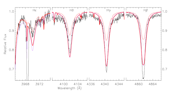
Figure 6: The HRS spectrum of  EC 19529$-$4430 in the vicinity of four Balmer lines compared with models for (a) a best-fit hydrogen abundance ($n_{\rm H}\approx 0.004$; thin lines) and (b) a fixed value of the hydrogen abundance ($n_{\rm H}=0.008$; thick lines). Solid red lines show the best-fit with non-LTE hydrogen and helium ($\mbox{\,\em T${}_{\rm eff}$}=20.7$ kK, $\mbox{\,log $g$}=3.5$). Dotted violet lines show H and He in LTE ($\mbox{\,\em T${}_{\rm eff}$}=19.8$ kK, $\mbox{\,log $g$}=3.4$). The strong narrow line at 3968.5Å is due to interstellar calcium.

4.3 Departures from LTE

A criticism of the LTE approximation is that it does not perform well in the cores of strong lines (Przybilla et al., 2005; Pandey & Lambert, 2011; Kupfer et al., 2017; Pandey & Lambert, 2017). This problem is mitigated by the use of models in which the hydrogen and helium level populations are treated in non-LTE (bold symbols in Fig. 2). For mixture m13n10 and $\xi_{\rm turb}=5$ $\mbox{km}\,\mbox{s}^{-1}$, the non-LTE solution (m13n) for the HRS spectrum is some 1400 K hotter than the equivalent LTE solution (v05). It is also successful in fitting the Hei line cores much better than the LTE solution (Fig. 5).

Since the underlying models are computed with independent codes, it is necessary to verify that the difference comes primarily from the non-LTE treatment of H and He lines, and not from other differences between the underlying models. Fig. 4 compares the temperature structures of models computed with sterne and tlusty for identical input parameters. Within the line-forming region ($10^{-4}<\tau_{4000}<1$) the temperatures differ by less than 1%. A separate grid of models for the mixture mixture m13n10 and $\xi_{\rm turb}=5$ $\mbox{km}\,\mbox{s}^{-1}$was computed using tlusty and synspec in which the H and He lines were treated in LTE. Fitting the HRS spectrum to this grid gave a solution almost identical to that for the equivalent grid calculated with sterne and spectrum. This solution is labelled ‘m13s’ in Fig. 2. Equivalence between the tlusty+synspec and sterne+spectrum solutions in LTE is also demonstrated in Fig. 5, particularly in the cores of the diffuse ($2P^{0}-nD$) lines.

To address the question of how much the line cores affect the fits, the central 2Å of all Hei lines were excluded. For the reference sterne$+$spectrum grid m13n10 (v05), $T_{\rm eff}$ and $g$ increased to almost exactly the values given by the tlusty and synspec (non-LTE) grid with the line cores included. However, excluding the line cores from the non-LTE grid increased $T_{\rm eff}$ by a similar amount $\approx 1\,000$ K, implying that the line wings are also significantly different.

4.4 Formal and systematic errors

It is difficult to assign confidences to our solutions; small changes in fit settings, such as wavelength range, wavelength weighting and normalization, can produce changes an order of magnitude larger than the formal errors in the $\chi^{2}$ minimization. In most cases, we check for global minima by restarting the fit with different initial estimates and checking that same solutions are obtained. The formal errors for the HRS solutions have maxima of 50 K in $T_{\rm eff}$ and 0.01 dex in $g$. The correlation between $T_{\rm eff}$ and $g$ is robust over different spectra and different model grids.

Microturbulent velocity is not too important for the $T_{\rm eff},g$ solution so long as some line broadening is included; the results for v05, v10 and v15 (mix m13n10) are almost coincident, whilst being substantially hotter than for ${\bf v00}$. HRS results for m20, m10 and p00 in Fig. 2 are diverse for decadal changes in metallicity but, if the metallicity is about right, other factors are probably more important. The LTE results for m10 and m13n10 (v05) are comparable, as are the non-LTE results for the same mixtures.

4.5 RSS

Solutions were obtained for the same model grids and for the RSS spectrum; for clarity only three solutions are shown in Fig. 2 (black diamonds), being for the m13n10 (diamond+square), m10 (diamond+cross) and m13n10_nlte (bold diamond) grids.

In comparing HRS and RSS results, the influence of weak lines at lower resolution is reduced; exactly why this favours higher $T_{\rm eff}$ and $g$ is unclear. Excluding Balmer lines and sharp Hei and H lines from the HRS fits reduced $T_{\rm eff}$ by 400 K, with no effect on gravity.

Both the LTE and non-LTE RSS results are consistent with the non-LTE HRS results. The former seems counter-intuitive, but a test using the fully LTE tlusty $+$ synspec grid gave a much lower $T_{\rm eff}\approx 18\,900$ K, suggesting that systematic errors in fitting the RSS spectrum remain significant.

4.6 Hydrogen abundance.

In a free solution, the hydrogen abundance measured from H$\beta,\gamma,\delta$ and $\epsilon$ is $\approx 0.5\%$ by number. Forcing the solution to fit H$\gamma$ yields $\approx 0.8\%$. However, in both LTE and non-LTE solutions, the Balmer line fits are inconsistent in the sense that, if a model spectrum matches at H$\gamma$, the model for H$\beta$ is too weak and the models for H$\delta$ and H$\epsilon$ are increasingly too strong (Fig. 6).

The blue squares in Fig. 2 represent fits to the HRS spectrum in which $n_{\rm H}=0.008$ was held fixed. Otherwise the symbols match the corresponding red triangles; i.e. ‘$\times$’ = m10, ‘$\square$’ = m13n10 v05, and a bold symbol = m13n10_nlte.

Both Przybilla et al. (2005) and Pandey & Lambert (2017) were able to resolve this ‘Balmer-line’ problem through the use of non-LTE models. This has not been possible in the current case.

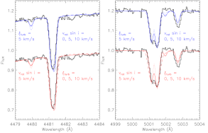
Figure 7: The HRS spectrum of  EC 19529$-$4430 in the vicinity of Mgii 4481Å and Nii 5001Å doublets compared with a model spectrum for 3 different values of projected rotation velocity $v_{\rm rot}\sin i$ (top - blue) and microturbulent velocity $\xi_{\rm turb}$ (bottom - red). Values are indicated by dots $=0$ $\mbox{km}\,\mbox{s}^{-1}$, solid lines $=5$ $\mbox{km}\,\mbox{s}^{-1}$and dashes $=10$ $\mbox{km}\,\mbox{s}^{-1}$.

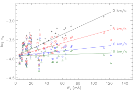
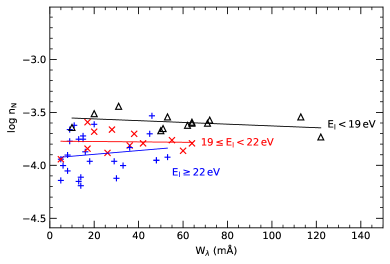
Figure 8: Top: Abundances derived from Nii lines as a function of equivalent width for microturbulent velocities of $\xi_{\rm turb}=0,5,10$ and 15 $\mbox{km}\,\mbox{s}^{-1}$. The base model atmospheres used were m13n10/h01he99/t200g350 with input $\xi_{\rm turb}=0$, 5, 10 and 15 $\mbox{km}\,\mbox{s}^{-1}$. The solid lines show a linear regression for each value of $\xi_{\rm turb}$. Bottom: The same for $\xi_{\rm turb}=7$  $\mbox{km}\,\mbox{s}^{-1}$, with the Nii lines separated into 3 groups ordered by $E_{\rm l}$

4.7 Rotation.

The Mgii 4481Å doublet is unresolved but asymmetric; a projected rotation velocity $v\sin i=5\pm 2$ $\mbox{km}\,\mbox{s}^{-1}$ is sufficient to match the observed profile (Fig. 7).

4.8 Microturbulent velocity.

Two methods have been considered to estimate the microturbulent velocity $\xi$. Looking at line profiles, the resolved Nii 5001 Å doublet requires a value of $\xi_{\rm turb}$ between 5 and 10  $\mbox{km}\,\mbox{s}^{-1}$  (Fig. 7). The larger value produces profiles that are broader than observed; the lower value matches the line wings but over-resolves the doublet core. Alternatively, $\xi_{\rm turb}$ can be adjusted so that all of the Nii lines yield a consistent nitrogen abundance across the full range of measured equivalent widths. This method indicates $\xi_{\rm turb}=15\pm 5$ $\mbox{km}\,\mbox{s}^{-1}$(Fig. 8, upper panel). The conflict between these methods is partially resolved if the Nii lines are considered according to the excitation potential of the lower energy level of the transition $E_{l}$. The lines fall naturally into three groups, namely lines with (1) $E_{\rm l}<19$eV, (2) $19{\rm eV}<E_{\rm l}<22$eV, and (3) $E_{\rm l}>22$eV. A value $\xi_{\rm turb}=7\pm 1$ $\mbox{km}\,\mbox{s}^{-1}$ minimizes the absolute gradient ${\rm d}\log n_{\rm N}/{\rm d}W_{\lambda}$ averaged over all three groups (Fig. 8: lower panel). However, the inconsistency between lines of different $E_{l}$ suggests that the temperature structure of the atmosphere is still not fully solved or that some lines may show non-LTE effects.

Since the parameters derived from the spectral fits are relatively insensitive to $\xi_{\rm turb}>5$ $\mbox{km}\,\mbox{s}^{-1}$, this value is deemed acceptable for the model atmosphere calculation. Its principal effect on the model structure is through line opacity in the ultraviolet which is reduced by the relatively low metallicity of the star.

For measuring abundances, errors will not be too large if a low value of $\xi_{\rm turb}$ is adopted, so long as the line equivalent widths are small (e.g. $W_{\lambda}<50$mÅ). This would certainly be necessary if a spectral synthesis approach were to be used because otherwise the model profiles would be too broad to fit the observed profiles. On the basis of Fig. 8, we have used $\xi_{\rm turb}=7$ $\mbox{km}\,\mbox{s}^{-1}$ to measure abundances directly from measured equivalent widths using the individual line curve-of-growth method (Table B.2). For reference, the majority of lines used in our analysis have equivalent widths $<100$mÅ. The minimum measurable equivalent width depends on the local signal-to-noise ratio which varies throughout the èchelle spectrum, but generally $W_{\lambda}>4$mÅ. This corresponds roughly to the line detection threshold $W_{\lambda}>n^{2}\sigma_{a}^{2}/\delta\lambda=6.9$mÅ (Snowdon et al., 2022) for $\sigma_{4540}=0.006$ (Table 1), pixel width $\delta\lambda=0.05$Å and a confidence level of 99% ($n=3$).

4.9 Adopted solution.

The final surface properties measured for  EC 19529$-$4430 are $T_{\rm eff}=20\,700\pm(40,250)$ K and $\log g/{\rm cm\,s^{-2}}=3.49\pm(0.01,0.03)$, $n_{\rm H}=0.008\pm(0.0001,0.002)$ with $v\sin i=5\pm 2$ $\mbox{km}\,\mbox{s}^{-1}$. These are taken from the fit of the HRS spectrum to the tlusty $+$ synspec grid with mixture m13n10 and $\xi_{\rm turb}=5$ $\mbox{km}\,\mbox{s}^{-1}$. All elements are treated in LTE in the tlusty models. H and He are treated in non-LTE in the synspec formal solutions; other elements are in LTE. 1$\sigma$ errors are given in the form (statistical, systematic).

Table 2: Atmospheric abundances of  EC 19529$-$4430, helium stars with similar $L/M$ ratios, and the Sun. Abundances are given as $\log\epsilon$, normalised to $\log\Sigma\mu\epsilon=12.15$. A colon indicates an uncertain value. Ratios relative to the Sun are shown for  EC 19529$-$4430 beneath.

Star	H	He	C	N	O	Ne	Mg	Al	Si	P	S	Ar	Fe	Ref
$\log\epsilon$
EC 19529$-$4430	9.24	11.54	5.60	7.76	6.67		6.50	4.95	5.89		5.99		6.11
$\pm$	0.10		0.22	0.19	0.12		0.12	0.15	0.12		0.25		0.11
V652 Her	9.61	11.54	7.29	8.69	7.58	7.95	7.80	6.12	7.47	:6.42	7.05	6.64	7.04	1,2
V652 Hera	9.5	11.5	7.0	8.7	7.6	8.1	7.1		7.4		7.4		7.1	3
J1846$-$4138	9.56	11.54	6.91	8.69	7.78	8.29	7.91	6.44	7.61	5.62	6.93		7.07	4
BX Cir	8.1	11.5	9.02	8.4	8.0			7.2	6.0	6.8	5.0	6.6	6.6	5
BD $+10^{\circ}2179$	8.36	11.53	9.75	8.03	7.51	8.00	6.97	5.84	7.14		6.84		6.55	6
Sun	12	10.93	8.43	7.83	8.69	7.93	7.60	6.45	7.51	5.45	7.12	6.40	7.50	7
$\log\epsilon/\epsilon_{\odot}$
EC 19529$-$4430	$-2.76$	0.61	$-2.83$	$-0.07$	$-2.02$		$-1.10$	$-1.50$	$-1.62$		$-1.13$		$-1.39$

References. 1 Jeffery et al. (1999b), 2: Jeffery et al. (2001), 3: Pandey & Lambert (2017), 4: Jeffery (2017), 5: Drilling et al. (1998), 6: Kupfer et al. (2017), 7: Asplund et al. (2009).

Note. (a) non-LTE measurements

4.10 Elemental Abundances

Elemental abundances were computed for each measured absorption line using individual curves-of-growth computed with spectrum. Two values were calculated for each line with model atmospheres from grid m13n10 having $\mbox{\,$T_{\rm eff}$}=20\,000$ and $22\,000$ K, and otherwise $\log g=3.50$, $n_{H}=0.01$ and $\xi_{\rm turb}=5$ $\mbox{km}\,\mbox{s}^{-1}$. Abundances were computed with $\xi_{\rm turb}=7$ $\mbox{km}\,\mbox{s}^{-1}$, as indicated in § 4.8, and errors were propagated from the equivalent width errors to the abundances on a line-by-line basis. Line abundances and errors were interpolated to $\mbox{\,$T_{\rm eff}$}=20\,700$ K. Results for each line and each ion are shown in Appendix B (Table B.4).

The overall elemental abundances of measured species are given in Table 2 and are compared with abundances for other relatively high-gravity extreme helium stars and the Sun. Where lines from more than one ion species are present, the overall elemental abundance is calculated from the weighted mean over all lines of that element.

We note the very low abundances of magnesium, aluminium, silicon, sulphur and iron, indicative of a systemically low metallicity, $-1.53<\log\epsilon_{i}/\epsilon_{\odot}<-0.87$, ${\rm Z}_{i}\in$(Mg,Al,Si,S,Fe). We have adopted $-1.3$ as an indicative mean.

We also note the ratio C : N : O $\approx 1:100:8$. This ratio is $4:90:7$ in V652 Her, and $1:88:11$ in J1846$-$4138.

Fluorine is an important stellar evolution tracer (Pandey, 2006; Bhowmick et al., 2020). The crucial Fii lines in the optical ultraviolet were undetectable in V652 Her; Bhowmick et al. (2020) could only deduce an upper limit of 10 times the solar abundance. Our spectrum does not reach these lines.

An independent check on the effective temperature is provided by the ionization equilibria of species where lines from more than one ion are present. Equilibrium is defined as the model effective temperature where the abundances derived from each ion would be equal. This was computed for Si ii/iii yielding $T_{\rm ion}=21\,550\pm 820$ K and for S ii/iii yielding $T_{\rm ion}=20\,000\pm 570$ K.

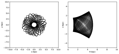
Figure 9: galpy orbit for  EC 19529$-$4430 computed for 3 Gyrs from its current positions. The panels show motion in the $\rm X-Y$ (left) and $\rm R-Z$ (right) planes, with the Galactic centre being at the origin.

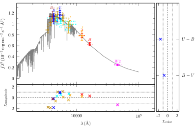
Figure 10: The spectral energy distribution of  EC 19529$-$4430 and model fit (grey line) with $T_{\rm eff}=20\,700\,{\rm K}$ (upper panel). The lower panel shows the residuals. Photometry is taken from:   Bianchi et al. (2017)(FUV,NUV),  Høg et al. (2000)(B_T,V_T),  Henden et al. (2015)(B,V),  Riello et al. (2021)($\rm G_{BP},\,G,\,G_{RP}$),  Onken et al. (2019)(u,v,g,r,i,z),  Denis (2005)(I,J),  Cutri et al. (2003)(J,H) and Schlafly et al. (2019)(W2).

5 Distance and Kinematics

5.1 Kinematics

From an analysis of EHe kinematics using Gaia eDR3 (Gaia Collaboration et al., 2016; Gaia Collaboration, 2021) data, Pandey et al. (2021) found that EHes belong to a spherical population that is more extended than the R CrB stars (RCBs) to which they were being compared. Extending earlier work by Martin (2019) and using positions and proper motions from Gaia DR3 (Gaia Collaboration et al., 2016; Gaia Collaboration, 2023), Philip Monai et al. (2023) presented a more detailed study of EHe kinematics, distinguishing between the disk (thin/thick disk stars) and the spherical components (halo/bulge stars). They found that EHes are present in all Galactic populations. Tisserand et al. (2023) studied a large sample of RCBs, dustless hydrogen-deficient carbon stars (HDCs) and EHes. They came to no conclusion about the RCB distribution due to uncertainties arising from the Gaia point-spread function, but concurred that HdCs and RCBs are to be found in all four Galactic components. Both Philip Monai et al. (2023) and Tisserand et al. (2023) support the idea that EHes formed recently from double white-dwarf mergers that arise originally from binary star formation over a range of epochs.

Philip Monai et al. (2023) obtained a distance to  EC 19529$-$4430  of $4.4^{+1.2}_{-0.8}$ kpc. Although the error is non-negligible ($\approx 22\%$), its retrograde orbit clearly makes  EC 19529$-$4430 a halo member (Fig. 9). This is consistent with its low overall metallicity.

5.2 Spectral Energy Distribution

Philip Monai et al. (2023) used measurements of the spectral energy distribution (SED) to obtain radii and luminosities for all of the EHes. These measurements have been repeated for  EC 19529$-$4430 using a more appropriate grid of model atmospheres (m13n10) and  $T_{\rm eff}$ and  log $g$ as given by the model atmosphere analysis (Fig. 10). The results are only marginally different to those given by Philip Monai et al. (2023). With color excess $E(44-55)=0.067\pm 0.011$mag being the only free parameter in the SED fit, the angular diameter is given as $\log\theta/{\rm rad}=-10.494\pm 0.007$. At the Gaia distance, this yields a median radius of $3.4^{+1.0}_{-0.6}$ $\rm R_{\odot}$ and luminosity $1.9^{+1.2}_{-0.6}\times 10^{3}$ $\rm L_{\odot}$. With substantial errors in both distance and gravity, the median mass of $1.3^{+0.8}_{-0.5}$ $\rm M_{\odot}$is not well constrained. Using modes rather than medians reduces all of the above values by some 30%.

Philip Monai et al. (2023) concluded that EHes may be divided into high- and low-luminosity groups, which may be associated with different types of progenitor, namely CO+He and He+He double white dwarf mergers respectively. Both groups include members from the galactic thin disk, the galactic thick disk and the galactic halo.

 EC 19529$-$4430 is marginal in terms of luminosity, being at the upper limit of the low-luminosity group. However, its high nitrogen abundance strongly suggests that  EC 19529$-$4430 belongs to the low luminosity group, which also includes the N-rich EHe stars V652 Her and J1846$-$4138. C-poor and N-rich surfaces are only expected for some He+He mergers, and not for He+CO mergers. C-rich and N-rich surfaces are expected for He+CO mergers and the more massive He+He mergers (Zhang & Jeffery, 2012).

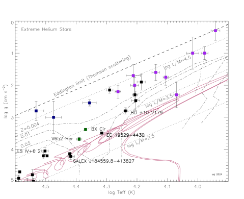
Figure 11: The $g-T_{\rm eff}$ diagram for  EC 19529$-$4430 with reference to other known extreme helium stars. The positions of the Eddington limit (Thomson scattering: dashed), luminosity-to-mass contours (solar units: dotted) and lower boundaries for pulsation instability (metallicities $Z$ = 0.004, 0.01, 0.03: dot-dashed) (Jeffery et al., 1999b) are also shown. Variable EHes are shown in purple (cool), blue (hot) and green (V652 Her like variables). Non-variables are black. Data for $T_{\rm eff},g$ are as in Jeffery (2008), (Ahmad & Jeffery, 2003) or Jeffery et al. (2021), except for BD+10^∘2179 (Kupfer et al., 2017),  GALEX J184559.8$-$413827 (Jeffery, 2017), BPS CS 22940–0009 (Snowdon et al., 2022) and  EC 19529$-$4430. Post-merger evolution tracks for models of He+He white dwarf mergers (Zhang & Jeffery, 2012, 0.30+0.25 and 0.30+0.30 $M_{\odot}$) are shown in red. Stars from Table 2 and other selected stars from the low-mass sequence identified by Philip Monai et al. (2023) are labelled.

6 Conclusion

We have presented a fine analysis of the spectrum of the recently discovered extreme helium star  EC 19529$-$4430. In doing so, we have examined the impact of several assumptions inherent in the model atmosphere approach, including the metallicity, the microturbulent velocity and departures from LTE. All three, if not correctly treated, can have a significant impact on the final result, amounting cumulatively in this case to over 3 000 K (or $>10\%$) in  $T_{\rm eff}$. Treating the neutral helium lines in non-LTE, and metal line-blanketing with an appropriate metallicity and microturbulent velocity, we obtain a solution for  $T_{\rm eff}$ and  log $g$ which is consistent over several discriminants. Citing the systematic errors, we conclude that $T_{\rm eff}=20\,700\pm 250$ K and $\log g/{\rm cm\,s^{-2}}=3.49\pm 0.03$. The surface hydrogen abundance cannot be obtained consistently from all four Balmer lines measured; 0.8% by number is given by the H$\gamma$ line, but a mean value between 0.45% and 1% is possible. Otherwise, the surface composition is predominantly metal-poor, with $\log\epsilon_{\rm Fe}/\epsilon_{\odot}=-1.39$, or $\langle\log\epsilon_{i}/\epsilon_{\odot}\rangle\approx-1.3$ for ${\rm Z}_{i}\in$(Mg,Al,Si,S,Fe). For such a metal-poor mixture, nitrogen is 1.2 dex overabundant. Since carbon and oxygen are 1.5 and 0.7 dex underabundant, respectively, with respect to the mean metallicity, the surface appears to be composed primarily of CNO-processed helium. Kinematically,  EC 19529$-$4430 is a galactic halo star in a retrograde orbit.

Fig. 11 shows  EC 19529$-$4430 relative to other EHes in a $\log g-\log\mbox{\,$T_{\rm eff}$}$ diagram. Contours of similar $L/M$ ratio run diagonally across this figure. Philip Monai et al. (2023) argued that the distribution of EHes in this figure suggests the presence of low and high $L/M$ sequences. The former are consistent with evolutionary tracks for merging He+He white dwarfs (Zhang & Jeffery, 2012). These form originally from binary star systems in which both components expand at the end of core-helium burning. If sufficiently close, they will interact in a common envelope. One or more common-envelope phases will remove material from both stars and shrink the orbit to leave a double white dwarf (DWD) binary. The overall age of  EC 19529$-$4430 is thus dominated by the main-sequence lifetime of the progenitor binary and the gravitational wave radiation timescale between DWD formation and merging. Both are determined by the mass ratios and separations of the initial main-sequence stars and of the two white dwarfs. On the basis of binary-star population synthesis calculations by Yu & Jeffery (2010, 2011), Philip Monai et al. (2023) argued that approximately 50% of EHes formed in the current epoch should come from He+He WD binaries in the galactic halo. Zhang & Jeffery (2012) demonstrated that the more massive He+He merger products should be carbon-rich and nitrogen-rich, whilst the less massive products would red carbon-poor and nitrogen-rich. This model therefore provides a good description of  EC 19529$-$4430, consistent with its surface composition, galactic orbit, and position in the $\log g-\log\mbox{\,$T_{\rm eff}$}$ diagram.

 EC 19529$-$4430 is the most metal-poor EHe star known. It is the coolest member of the carbon-poor group, of which V652 Her and J1846-4138 are slightly warmer metal-rich analogues. Hotter carbon-poor EHe stars are found as subdwarfs. The non-detection of pulsations is probably associated with the iron abundance being too low to drive pulsations. There is no evidence for a binary companion either from radial velocities or the spectra energy distribution. It is most likely that  EC 19529$-$4430 formed from the merging of two helium white dwarfs, which themselves formed as a binary system some 11 Gyr ago, and that it will evolve to become a core helium-burning EHe subdwarf. It will be important to identify cooler N-rich EHe stars, additional metal-poor EHe stars, and to study other chemical species, such as neon, to better understand the He+He WD merger process.

Data Availability

The SALT and TESS data reported in this paper are available in their respective public archives (ssda.salt.ac.za, and archive.stsci.edu/missions-and-data/tess). Theoretical model atmospheres and spectra generated for this paper will be made available on reasonable request to the principal author.

Appendix A Model Atmosphere Grids

Details for each of the model atmosphere grids used in § 4 are given in Table A.3.

Table A.3: Identifiers, chemical composition and other parameters for model atmosphere grids used in § 4. Where different, labels used in Fig. 2 are given in parentheses.

Label	Code	$n_{\rm N}$	[Fe/H]	$\xi_{\rm turb}$	Lines	Comment
p00	sterne+spectrum	$\odot$	0.0	5		LTE + scattering
m10	sterne+spectrum	$\odot/10$	$-1.0$	5		LTE + scattering
m20	sterne+spectrum	$\odot/100$	$-2.0$	5		LTE + scattering
m13n10v00 (v00)	sterne+spectrum	$\odot$	$-1.3$	0		LTE + scattering
m13n10v05 (v05)	sterne+spectrum	$\odot$	$-1.3$	5		LTE + scattering
m13n10v10 (v10)	sterne+spectrum	$\odot$	$-1.3$	10		LTE + scattering
m13n10v15 (v15)	sterne+spectrum	$\odot$	$-1.3$	15		LTE + scattering
m10_nlte (m10n)	tlusty+synspec	$\odot/10$	$-1.0$	5		model LTE, H + Hei lines nLTE
m13n10_nlte (v05n)	tlusty+synspec	$\odot$	$-1.3$	5		model LTE, H + Hei lines nLTE
m13n10_lte (v05s)	tlusty+synspec	$\odot$	$-1.3$	5		LTE

Table B.4: Equivalent widths and scaled abundances for unblended absorption lines in the spectrum of  EC 19529$-$4430.

Ion	Reference
$\lambda$	$E_{\rm l}$	$\log gf$	$W_{\lambda}$	$\sigma_{W_{\lambda}}$	$\log\epsilon_{i}$	$\sigma_{\log\epsilon_{i}}$
Å	eV		mÅ	mÅ
N ii	Becker & Butler (1989)
3919.01	20.410	$-$0.335	36	20	7.70	0.38
3955.85	18.466	$-$0.780	50	20	7.85	0.31
3995.00	18.498	0.225	122	26	7.78	0.29
4035.08	23.120	0.597	30	12	7.38	0.25
4041.31	23.128	0.830	53	21	7.57	0.31
4056.90	23.140	$-$0.461	11	8	7.89	0.36
4073.05	23.124	$-$0.160	20	11	7.89	0.32
4082.27	23.132	0.150	19	11	7.55	0.34
4171.60	23.196	0.280	14	7	7.31	0.27
4173.57	23.240	$-$0.457	5	4	7.57	0.38
4176.16	23.196	0.600	33	10	7.49	0.21
4179.67	23.250	$-$0.204	13	8	7.76	0.30
4195.97	23.242	$-$0.290	8	6	7.61	0.36
4199.98	23.246	0.030	16	7	7.63	0.24
4227.74	21.600	$-$0.089	26	12	7.62	0.29
4236.93	23.239	0.383	46	13	7.96	0.22
4237.05	23.242	0.553	45	13	7.79	0.22
4241.18	23.240	$-$0.336	9	5	7.73	0.29
4241.76	23.242	0.210	47	12	7.54	0.20
4242.44	23.240	$-$0.336	6	4	7.51	0.32
4417.10	23.415	$-$0.340	9	5	7.84	0.29
4427.24	23.420	$-$0.004	8	9	7.45	0.54
4431.82	23.410	$-$0.152	5	4	7.36	0.39
4432.74	23.410	0.595	29	10	7.53	0.22
4433.48	23.420	$-$0.028	15	5	7.77	0.19
4442.02	23.420	0.324	14	5	7.39	0.21
4447.03	20.411	0.238	64	10	7.70	0.14
4530.40	23.470	0.671	36	6	7.65	0.13
4601.48	18.468	$-$0.385	71	14	7.90	0.19
4607.16	18.464	$-$0.483	64	15	7.90	0.21
4613.87	18.468	$-$0.607	51	11	7.85	0.17
4621.29	18.468	$-$0.483	62	10	7.88	0.13
4630.54	18.484	0.093	113	10	7.96	0.12
4643.09	18.484	$-$0.385	72	10	7.93	0.13
4667.21	18.497	$-$1.580	10	4	7.87	0.18
4678.14	23.572	0.434	13	4	7.34	0.16
4694.70	23.570	0.111	15	5	7.74	0.19
4774.24	20.650	$-$1.055	5	2	7.57	0.25
4779.72	20.650	$-$0.577	20	6	7.82	0.17
4788.13	20.650	$-$0.388	28	8	7.83	0.18
4803.29	20.660	$-$0.135	38	8	7.79	0.14
4987.38	20.940	$-$0.630	17	4	7.90	0.15
5001.13	20.646	0.282	55	8	7.72	0.23
5001.47	20.654	0.452	60	9	7.62	0.13
5002.70	18.480	$-$1.086	31	6	8.06	0.12
5007.33	20.940	0.161	42	7	7.69	0.13
5010.62	18.470	$-$0.611	53	12	7.95	0.18
5025.66	20.666	$-$0.438	17	5	7.65	0.17
5045.09	18.460	$-$0.389	65	14	7.90	0.19
5073.59	18.497	$-$1.280	20	7	7.99	0.20
					7.76	0.19
					$\mathrm{\Delta}\epsilon=-0.011$

Table B.4: (cont.)

Ion	Reference
$\lambda$	$E_{\rm l}$	$\log gf$	$W_{\lambda}$	$\sigma_{W_{\lambda}}$	$\log\epsilon_{i}$	$\sigma_{\log\epsilon_{i}}$
Å	eV		mÅ	mÅ
C ii	Yan & Seaton (1987)
4267.02$\rceil$	18.047	0.559
4267.27$\rfloor$	18.047	0.734	18	8	5.60	0.22
					5.60	0.22
					$\mathrm{\Delta}\epsilon=0.005$
O ii	Bell et al. (1994)
3973.26	23.442	$-$0.015	8	11	6.81	1.07
4072.15	25.650	0.552	5	5	6.58	0.90
					6.67	0.12
					$\mathrm{\Delta}\epsilon=-0.016$
Mg ii	Wiese et al. (1969)
4481.13$\rceil$	8.863	0.568
4481.15 $\arrowvert$	8.864	$-$0.560
4481.33$\rfloor$	8.863	0.732	110	15	6.50	0.12
					6.50	0.12
					$\mathrm{\Delta}\epsilon=0.035$
Al iii	Cunto et al. (1993)
4512.54	17.808	0.405	12	5	5.14	0.21
4529.20	17.740	0.660	12	4	4.84	0.16
					4.95	0.15
					$\mathrm{\Delta}\epsilon=-0.004$
Si ii	Becker & Butler (1990)
4128.07	9.837	0.369	18	9	6.02	0.28
4130.87	9.839	$-$0.824	22	9	5.93	0.21
5041.03	10.070	0.262	6	3	5.73	0.26
5055.98	10.070	0.517	8	3	5.60	0.22
					5.81	0.19
					$\mathrm{\Delta}\epsilon=0.031$
Si iii	Becker & Butler (1990)
4552.62	19.018	0.283	77	12	6.36	0.14
4567.82	19.018	0.061	55	10	6.31	0.14
4574.76	19.018	$-$0.416	30	7	6.34	0.14
4716.65	25.330	0.491	3	2	5.96	0.34
4813.30	25.980	0.702	4	2	6.05	0.28
4819.72	25.980	0.814	5	2	5.99	0.26
					6.27	0.15
					$\mathrm{\Delta}\epsilon=-0.008$
S ii	Wiese et al. (1969)
4815.55	13.672	0.177	7	3	5.87	0.17
5032.41	13.668	0.176	9	4	6.01	0.19
					5.93	0.07
					$\mathrm{\Delta}\epsilon=0.037$
S iii	Hardorp & Scholz (1970)
4253.59	18.244	0.400	17	7	5.80	0.26
4284.98	18.193	0.110	12	6	5.87	0.27
4332.69	18.188	$-$0.240	4	4	5.67	0.46
					5.81	0.08
					$\mathrm{\Delta}\epsilon=-0.011$
Fe iii	Kurucz & Petryemann (1975)
4164.73	20.634	0.972	5	4	5.95	0.38
4419.60	8.241	$-$2.207	10	5	6.18	0.24
					6.11	0.11
					$\mathrm{\Delta}\epsilon=0.011$

Appendix B Line Abundance Measurements

Table B.4 shows the abundances obtained from individual absorption lines in the spectrum of  EC 19529$-$4430. Columns 1 and 4 give wavelengths and equivalent widths ($W_{\lambda}$) for identified absorption lines. Multiplets treated as blends are grouped by a square bracket ”]” following the wavelength. Columns 2 and 3 give the excitation potential of the lower level ($E_{\rm l}$) and the oscillator strength ($\log gf$) for each transition. Column 5 gives the $1\sigma$ error in $W_{\lambda}$, as described by Snowdon et al. (2022). Lines with abundances $>2\sigma$ from the mean were rejected and omitted, and the means recalculated. The sources of oscillator strengths ($gf$) are given with the ion designation. Column 7 gives the abundance $\log\epsilon_{i}$ deduced from each line. Column 8 gives the error in the line abundance obtained by propagating $\sigma_{W_{\lambda}}$ through the abundance derivation in spectrum. The mean abundance for each ion is given as the weighted mean of all lines shown. Errors on the mean abundance per ion are given as the weighted standard deviation where the number of lines $n>2$, the semi-range where $n=2$, or the line measurement error where $n=1$. The change in abundance due to a systematic error $\delta\mbox{\,$T_{\rm eff}$}=+250$K is shown beneath the mean abundance in the form $\mathrm{\Delta}\epsilon={\rm d}\log\epsilon_{i}/{\rm d}T_{\rm eff}\times 250{\rm K}$.

Abundances were calculated at the adopted temperature of $T_{\rm eff}=20\,700$ K by interpolation, between LTE models with $\log g/{\rm cm\,s^{-2}}=3.50$, $\xi_{\rm turb}=7$  $\mbox{km}\,\mbox{s}^{-1}$, and $T_{\rm eff}$ of 20 000 and 22 000 K.

The Nii lines fall into three natural groups by $E_{\rm l}$ (see Fig. 8) with each group yielding a slightly different mean abundance. We compared the weighted mean from all lines taken together with the weighted mean for each group, namely lines with (1) $E_{\rm l}<19$eV, (2) $19{\rm eV}<E_{\rm l}<22$eV, and (3) $E_{\rm l}>22$eV and also groups (1)+(2) combined. Relative to the overall mean, the mean abundance for each group was (1) +0.21, (2) +0.01, (3) -0.10 and (1)+(2) +0.11 dex. Although it contains the largest number of lines, group (3) is dominated by weak lines with large abundance errors; it therefore has a smaller impact on the overall mean. Rather than reject any group of Nii lines, we have adopted the overall mean for the nitrogen abundance

Abundances for sulphur and silicon are available for 2 ions in each case. The abundances for Sii and Siii differ by 0.12 dex, which is within the scatter of individual line measurements and less than the error in any individual line abundance. The abundances for Siii and Siiii differ by 0.46 dex; the individual line abundance errors are less than this whilst the scatter for each ion is $\approx 0.4$ dex. On this basis, Table 2 gives the overall sulphur and silicon abundances from the weighted mean of all lines of both species . Since the silicon abundance is dominated by the strong Siiii lines at 4553, 4568, and 4575Å, which frequently do show strong non-LTE effects, we note that the silicon abundance may be overestimated.

References

- Ahmad & Jeffery (2003) Ahmad A., Jeffery C. S., 2003, A&A, 402, 335
- Asplund et al. (2009) Asplund M., Grevesse N., Sauval A. J., Scott P., 2009, ARA&A, 47, 481
- Beauchamp et al. (1997) Beauchamp A., Wesemael F., Bergeron P., 1997, ApJS, 108, 559
- Becker & Butler (1989) Becker S. R., Butler K., 1989, A&A, 209, 244
- Becker & Butler (1990) Becker S. R., Butler K., 1990, A&A, 235, 326
- Behara & Jeffery (2006) Behara N. T., Jeffery C. S., 2006, A&A, 451, 643
- Bell et al. (1994) Bell K. L., Hibbert A., Stafford R. P., McLaughlin B. M., 1994, Phys. Scr, 50, 343
- Bhowmick et al. (2020) Bhowmick A., Pandey G., Lambert D. L., 2020, ApJ, 891, 40
- Bianchi et al. (2017) Bianchi L., Shiao B., Thilker D., 2017, ApJS, 230, 24
- Crawford et al. (2023) Crawford C. L., Tisserand P., Clayton G. C., Soon J., Bessell M., Wood P., García-Hernández D. A., Ruiter A. J., Seitenzahl I. R., 2023, MNRAS, 521, 1674
- Cunto et al. (1993) Cunto W., Mendoza C., Ochsenbein F., Zeippen C. J., 1993, å, 275, L5+
- Cutri et al. (2003) Cutri R. M., Skrutskie M. F., van Dyk S., et al. 2003, VizieR Online Data Catalog, 2246
- Denis (2005) Denis C., 2005, VizieR Online Data Catalog, p. B/denis
- Dimitrijevic & Sahal-Brechot (1984) Dimitrijevic M. S., Sahal-Brechot S., 1984, J. Quant. Spec. Radiat. Transf., 31, 301
- Dimitrijevic & Sahal-Brechot (1990) Dimitrijevic M. S., Sahal-Brechot S., 1990, A&AS, 82, 519
- Drilling (1980) Drilling J. S., 1980, ApJ, 242, L43+
- Drilling (1983) Drilling J. S., 1983, ApJ, 270, L13
- Drilling et al. (1998) Drilling J. S., Jeffery C. S., Heber U., 1998, A&A, 329, 1019
- Drilling et al. (2013) Drilling J. S., Jeffery C. S., Heber U., Moehler S., Napiwotzki R., 2013, A&A, 551, A31
- Gaia Collaboration (2021) Gaia Collaboration 2021, A&A, 649, A1
- Gaia Collaboration (2023) Gaia Collaboration 2023, A&A, 674, A1
- Gaia Collaboration et al. (2016) Gaia Collaboration Prusti T., de Bruijne J. H. J., Brown A. G. A., Vallenari A., Babusiaux C., Bailer-Jones C. A. L., Bastian U., Biermann M., Evans D. W., et al. 2016, A&A, 595, A1
- Green et al. (1986) Green R. F., Schmidt M., Liebert J., 1986, ApJS, 61, 305
- Hardorp & Scholz (1970) Hardorp J., Scholz M., 1970, ApJS, 19, 193
- Heber (1983) Heber U., 1983, A&A, 118, 39
- Henden et al. (2015) Henden A. A., Levine S., Terrell D., Welch D. L., 2015, in American Astronomical Society Meeting Abstracts #225 Vol. 225 of American Astronomical Society Meeting Abstracts, APASS - The Latest Data Release. p. 336.16
- Hill et al. (1981) Hill P. W., Kilkenny D., Schönberner D., Walker H. J., 1981, MNRAS, 197, 81
- Høg et al. (2000) Høg E., Fabricius C., Makarov V. V., Urban S., Corbin T., Wycoff G., Bastian U., Schwekendiek P., Wicenec A., 2000, A&A, 355, L27
- Hubeny et al. (2021) Hubeny I., Allende Prieto C., Osorio Y., Lanz T., 2021, arXiv e-prints, p. arXiv:2104.02829
- Hubeny & Lanz (1995) Hubeny I., Lanz T., 1995, ApJ, 439, 875
- Hubeny & Lanz (2017a) Hubeny I., Lanz T., 2017a, arXiv e-prints, p. arXiv:1706.01859
- Hubeny & Lanz (2017b) Hubeny I., Lanz T., 2017b, arXiv e-prints, p. arXiv:1706.01935
- Hubeny & Lanz (2017c) Hubeny I., Lanz T., 2017c, arXiv e-prints, p. arXiv:1706.01937
- Hummer et al. (1993) Hummer D. G., Berrington K. A., Eissner W., Pradhan A. K., Saraph H. E., Tully J. A., 1993, å, 279, 298
- Jeffery (1994) Jeffery C. S., 1994, CCP7 Newsletter on Analysis of Astronomical Spectra, 21, 5
- Jeffery (1998) Jeffery C. S., 1998, MNRAS, 294, 391
- Jeffery (2008) Jeffery C. S., 2008, Inf. Bull. Var. Stars, 5817, 1
- Jeffery (2017) Jeffery C. S., 2017, MNRAS, 470, 3557
- Jeffery et al. (1999a) Jeffery C. S., Hill P. W., Heber U., 1999a, A&A, 346, 491
- Jeffery et al. (1999b) Jeffery C. S., Hill P. W., Heber U., 1999b, A&A, 346, 491
- Jeffery et al. (2015) Jeffery C. S., Kurtz D., Shibahashi H., Starling R. L. C., Elkin V., Montañés-Rodríguez P., McCormac J., 2015, MNRAS, 447, 2836
- Jeffery et al. (2021) Jeffery C. S., Miszalski B., Snowdon E., 2021, MNRAS, 501, 623
- Jeffery & Saio (1999) Jeffery C. S., Saio H., 1999, MNRAS, 308, 221
- Jeffery et al. (2001) Jeffery C. S., Woolf V. M., Pollacco D. L., 2001, A&A, 376, 497
- Kilkenny et al. (1997) Kilkenny D., O’Donoghue D., Koen C., Stobie R. S., Chen A., 1997, MNRAS, 287, 867
- Kilkenny et al. (2015) Kilkenny D., O’Donoghue D., Worters H. L., Koen C., Hambly N., MacGillivray H., 2015, MNRAS, 453, 1879
- Kilkenny et al. (2016) Kilkenny D., Worters H. L., O’Donoghue D., Koen C., Koen T., Hambly N., MacGillivray H., Stobie R. S., 2016, MNRAS, 459, 4343
- Kniazev (2016) Kniazev A. Y., 2016, Technical report, MIDAS pipeline for HRS: the absolute accuracy of radial velocities. Southern Africa Large Telescope
- Kupfer et al. (2017) Kupfer T., Przybilla N., Heber U., Jeffery C. S., Behara N. T., Butler K., 2017, MNRAS, 471, 877
- Kurucz (1993) Kurucz R., 1993, ATLAS9 Stellar Atmosphere Programs and 2 km/s grid. Kurucz CD-ROM No. 13. Cambridge, 13
- Kurucz & Petryemann (1975) Kurucz R., Petryemann E., 1975, SAO Spec.Rep, 362
- Kurucz (1996) Kurucz R. L., 1996, in Adelman S. J., Kupka F., Weiss W. W., eds, M.A.S.S., Model Atmospheres and Spectrum Synthesis Vol. 108 of Astronomical Society of the Pacific Conference Series, Status of the ATLAS 12 Opacity Sampling Program and of New Programs for Rosseland and for Distribution Function Opacity. p. 160
- Kurucz & Bell (1995) Kurucz R. L., Bell B., 1995, Atomic line list. Kurucz CD-ROM, Cambridge, MA: Smithsonian Astrophysical Observatory, —c1995, April 15, 1995
- Lynas-Gray et al. (1984) Lynas-Gray A. E., Schönberner D., Hill P. W., Heber U., 1984, MNRAS, 209, 387
- Martin (2019) Martin P., 2019, PhD thesis, Trinity College Dublin
- Moehler et al. (1990) Moehler S., Richtler T., de Boer K. S., Dettmar R. J., Heber U., 1990, A&AS, 86, 53
- Naslim et al. (2010) Naslim N., Jeffery C. S., Ahmad A., Behara N. T., Şahìn T., 2010, MNRAS, 409, 582
- O’Donoghue et al. (2013) O’Donoghue D., Kilkenny D., Koen C., Hambly N., MacGillivray H., Stobie R. S., 2013, MNRAS, 431, 240
- Onken et al. (2019) Onken C. A., Wolf C., Bessell M. S., Chang S.-W., Da Costa G. S., Luvaul L. C., Mackey D., Schmidt B. P., Shao L., 2019, PASA, 36, e033
- Pandey (2006) Pandey G., 2006, ApJ, 648, L143
- Pandey et al. (2021) Pandey G., Hema B. P., Reddy A. B. S., 2021, ApJ, 921, 52
- Pandey & Lambert (2011) Pandey G., Lambert D. L., 2011, ApJ, 727, 122
- Pandey & Lambert (2017) Pandey G., Lambert D. L., 2017, ApJ, 847, 127
- Pandey et al. (2006) Pandey G., Lambert D. L., Jeffery C. S., Rao N. K., 2006, ApJ, 638, 454
- Philip Monai et al. (2023) Philip Monai A., Martin P., Jeffery C. S., 2023, MNRAS
- Przybilla et al. (2005) Przybilla N., Butler K., Heber U., Jeffery C. S., 2005, A&A, 443, L25
- Ralchenko & Kramida (2020) Ralchenko Y., Kramida A., 2020, Atoms, 8, 56
- Reindl et al. (2014) Reindl N., Rauch T., Werner K., Kruk J. W., Todt H., 2014, A&A, 566, A116
- Riello et al. (2021) Riello M., Angeli F. D., Evans D. W., et al. 2021, A&A, 649
- Saio & Jeffery (2000) Saio H., Jeffery C. S., 2000, MNRAS, 313, 671
- Saio & Jeffery (2002) Saio H., Jeffery C. S., 2002, MNRAS, 333, 121
- Schlafly et al. (2019) Schlafly E. F., Meisner A. M., Green G. M., 2019, ApJS, 240, 30
- Schöning & Butler (1989) Schöning T., Butler K., 1989, A&AS, 78, 51
- Scott et al. (2023) Scott L. J. A., Jeffery C. S., Farren D., Tap C., Dorsch M., 2023, MNRAS, 521, 3431
- Seaton et al. (1994) Seaton M. J., Yan Y., Mihalas D., Pradhan A. K., 1994, mnras, 266, 805
- Snowdon et al. (2022) Snowdon E. J., Scott L. J. A., Jeffery C. S., Woolf V. M., 2022, MNRAS, 516, 794
- Stobie et al. (1997) Stobie R. S., Kilkenny D., O’Donoghue D., et al. 1997, MNRAS, 287, 848
- Tisserand et al. (2022) Tisserand P., Crawford C. L., Clayton G. C., Ruiter A. J., Karambelkar V., Bessell M. S., Seitenzahl I. R., Kasliwal M. M., Soon J., Travouillon T., 2022, A&A, 667, A83
- Tisserand et al. (2023) Tisserand P., Crawford C. L., Soon J., Clayton G. C., Ruiter A. J., Seitenzahl I. R., 2023, arXiv e-prints, p. arXiv:2309.10148
- Vidal et al. (1973) Vidal C. R., Cooper J., Smith E. W., 1973, ApJS, 25, 37
- Warner (1967) Warner B., 1967, MNRAS, 137, 119
- Wiese et al. (1969) Wiese W. L., Smith M. W., Miles B. M., 1969, Atomic transition probabilities. Vol. 2: Sodium through Calcium. A critical data compilation. NSRDS-NBS, Washington, D.C.: US Department of Commerce, National Bureau of Standards
- Yan & Seaton (1987) Yan Y., Seaton M. J., 1987, Journal of Physics B Atomic Molecular Physics, 20, 6409
- Yu & Jeffery (2010) Yu S., Jeffery C. S., 2010, A&A, 521, A85+
- Yu & Jeffery (2011) Yu S., Jeffery C. S., 2011, MNRAS, 417, 1392
- Zhang & Jeffery (2012) Zhang X., Jeffery C. S., 2012, MNRAS, 419, 452