Sections and Chapters

Transformers for molecular property prediction: Lessons learned from the past five years

Abstract

Molecular Property Prediction (MPP) is vital for drug discovery, crop protection, and environmental science. Over the last decades, diverse computational techniques have been developed, from using simple physical and chemical properties and molecular fingerprints in statistical models and classical machine learning to advanced deep learning approaches. In this review, we aim to distill insights from current research on employing transformer models for MPP. We analyze the currently available models and explore key questions that arise when training and fine-tuning a transformer model for MPP. These questions encompass the choice and scale of the pre-training data, optimal architecture selections, and promising pre-training objectives. Our analysis highlights areas not yet covered in current research, inviting further exploration to enhance the field’s understanding. Additionally, we address the challenges in comparing different models, emphasizing the need for standardized data splitting and robust statistical analysis.

Saarland University] Data Driven Drug Design, Center for Bioinformatics, Saarland University, Germany Equal Contribution Equal Contribution BASF] BASF SE, Ludwigshafen. Germany Saarland University] Data Driven Drug Design, Center for Bioinformatics, Saarland University, Germany

1 Introduction

Modern deep learning architectures are enabling applications across various domains. Architectures originally developed for computer vision ^{1, 2} and language processing ³ are reshaping central life science fields ^{4, 5}. These successes raise high expectations for the long-standing challenge of small molecule property prediction. Molecular property prediction (MPP) methods have a wide range of applications, including drug discovery, material science, crop protection, and environmental science. Accurate predictions of properties like on-target activity, physico-chemical properties, or (eco-)toxicity of the molecule ⁶ can help researchers prioritize compounds for further experimentation, assess the potential toxicity of chemicals, optimize drug candidates, and design new materials with desired properties ^{7, 8, 9}.

A key problem in the field of molecular property prediction is to find a molecular representation that corresponds well with relevant properties ⁹. An interesting difference between deep learning methods to more traditional quantitative structure-activity relationship (QSAR) modeling ¹⁰ is that representations can be learned from data instead of using fixed or human-engineered representations ^{11, 9}. For decades, fixed representations, such as molecular descriptors and fingerprints, have been employed to describe a molecule by converting it into a fixed vector length for using it in machine learning algorithms. Molecular descriptors can include physico-chemical properties, topological indices, and quantum chemistry properties. They provide a straightforward representation but are limited due to a priori selection. A special type of descriptors are molecular fingerprints, usually binary bit strings representing the presence or absence of substructures or functional groups in a molecule^{12, 13}. Popular examples are the extended-connectivity fingerprint (ECFP) ¹⁴, which represents atom environments, and MACCS structural keys, which encode substructures ¹⁵.

Multiple deep learning architectures have been proposed for supervised learning for MPP ^{16, 17}. Graph neural networks and graph convolutional neural networks ¹⁸ can learn from molecular graphs representing atoms and their connections ^{7, 19}. Another approach is the use of recurrent neural networks ²⁰ to model sequential molecule data, such as SMILES ²¹ strings ^{22, 9}. Generative models, like variational autoencoders ²³, generative adversarial networks ²⁴ and normalizing flow models ²⁵, are also employed for molecular property prediction. These models learn to embed the input molecule data into a latent space to generate novel molecules with desired properties by sampling from the latent space representation ^{22, 26, 27, 28, 29, 30, 31}. Transfer learning ³² is another promising technique. By training a deep learning model on one task with a sufficiently large data set of molecular structures and property labels, the model can learn general features transferable to a specific task with few labeled training data ^{33, 34, 35}.

However, labeled molecular property data sets are notoriously small, containing only hundreds or thousands of molecules ^{6, 11, 36, 9}. This small size limits supervised learning algorithms to derive potent representations for all properties of interest. Self-supervised learning (SSL) ³⁷ has emerged as a potential solution to overcome this bottleneck by exploiting the large corpus of unlabeled molecular data, which has been explored on SMILES ^{38, 39, 40, 41, 42} and molecular graphs ^{43, 44, 45}. SSL aims to learn general-purpose features or task-agnostic representations, meaning these representations can be reused in downstream tasks as proposed by BERT ⁴⁶. SSL approaches the feature extraction problem with a pre-training task (or pretext task), for example, with the objective of predicting missing parts in a masked input data point ⁴⁷. This approach is currently explored with great effort in the chemical domain ^{38, 39, 40, 41, 42, 43, 45, 48}. Still, standard machine learning models and features, like tree-based methods with fixed-size molecular fingerprints, remain strong baselines for real-world data sets ^{11, 49, 9}. This illustrates certain challenges that need to be overcome to exploit the full potential of deep learning models in this field.

Transformers³ are interesting architectures for molecular property prediction applications. They were developed originally for language processing and rely on sequential input and output. They have been a central component in the breakthrough of AlphaFold2 and other methods in the related field of protein structure prediction from the primary sequence ^{4, 5, 50}. Proteins’ sequential nature, i.e. their amino acid sequence, makes them an appropriate basis for developing protein language models. Accordingly, the expectations for extending this success to property prediction of other biomolecules are raised. For small molecules, the widely-used SMILES ²¹ strings are an intuitive sequential molecular encoding ready to be used with language models. The attention mechanism ⁵¹ used by transformers aims to learn context-dependent relationships and might be suited to capture complex non-additivities⁵² in molecular data. In addition, their encoder-decoder architecture is suitable for both molecular property prediction and molecule generation and they are the foundation for powerful architectures in computation linguistics ^{46, 53}. Transformers have also been shown to scale well to enormously large unlabeled data sets ^{46, 54}.

In this review, we aim to give an overview of the current state of transformer models for molecular property prediction (MPP). We first present the transformer architecture, its variants from the language domain, and their adaptions for MPP, which we categorize by their architectural differences. In the second section, we overview the data sets used for training and evaluation and examine the reported prediction performances. We then review the choices to consider when implementing a transformer model for MPP and discuss architectural choices, training objectives, and data set sizes. Finally, we describe the challenges encountered during this review, highlighting the need for a unified benchmark and reporting, and we provide potential next steps for using transformers for MPP.

2 The transformer model

The transformer model is a sequence-to-sequence model with the main aim of translating an input sequence into an output sequence. This concept has been utilized for different tasks in NLP, such as machine translation or text summarization ³, as well as tasks in cheminformatics such as reaction prediction ⁴⁸ and molecular optimization ⁵⁵. In this section, we will explain the transformer model and some of its variants, followed by outlaying the chemical language models derived from it (Figure 1).

Figure 1: An overview of the transformer model and where each chemical language model fits. The transformer model with the encoder-decoder modules is a sequence-to-sequence model that can be used for tasks like reaction prediction. However, each module can be used independently to provide more specialized performance. For example, the encoder module can be used to predict properties, while the decoder module can be used to generate novel molecules.

2.1 How transformer models work

The transformer model proposed by Vaswani et al. ³ took the field of natural language processing (NLP) by storm as the current citation for this work is over 100K ⁵⁶. The model consists of stacks of encoders and decoders that rely mainly on the previously used attention mechanism ⁵¹. This dispensed the need for using recurrent or convolutional neural networks (RNN and CNN), which were the SOTA prior to the transform model ³. Relying mainly on the attention mechanism allowed for parallel processing of the input sequence, which was previously hindered, for example, due to the sequential nature of RNNs. This enabled a significant reduction in computation time as well as processing longer sequences which enables learning longer-range dependencies.

The attention mechanism proposed by Vaswani et al. ³ relies on a scaled dot product of three linear transformations that are named the query (Q), key (K), and value (V) vectors. These vectors are of length $d_{k}$ which are calculated for each input sequence and attention is performed as follows:

$$Attention(Q,K,\ and\ V)=softmax(\dfrac{QK^{T}}{\sqrt{d_{k}}})V$$

Besides the attention mechanism, the transformer model comprises layer normalization steps that stabilize calculations and a feed-forward neural network which is the only source of non-linearity in the model. The input to the encoder model is a tokenized sequence. I.e., the input sequence is broken into composing units called tokens, which can be characters, words, subwords, etc., depending on the tokenization method (see Figure 1).

The transformer model’s encoder unit focuses on identifying a token’s relationship to its surrounding tokens, including previous and following tokens, which is done via self-attention. However, the decoder subunit is a generative module that focuses on predicting the next token from strictly processing the previous tokens only. The decoder uses masked self-attention for this task as the future words for each token are masked. Additionally, the decoder’s generation task is offset by one token to allow for the output embeddings of the encoder module to be processed by the decoder module. At this step, a third attention type called cross-attention is performed, which computes the relationship of the decoder’s generated tokens to the encoder’s contextualized embeddings of the input tokens. This cross-attention step allows for both the encoder and the decoder to align their predictions between the input sequence and the desired output sequence. For example, in the case of the original transformer model ³, the goal was machine translation between different languages.

In addition to reducing computation cost and detecting longer-range dependencies, the transformer model paved the way for the pre-training and fine-tuning paradigm as proposed in BERT ⁴⁶. In this paradigm, the model is trained on a large unlabeled data set with objectives that allow the model to form a general comprehension of the training domain. Afterward, the pre-trained model can be tuned on the labeled - but significantly smaller - downstream data set. The transformer models have enabled the training of foundational models that can easily be fine-tuned for numerous downstream data sets.

Although the architecture of the transformer model makes it a sequence-to-sequence model, the individual encoder and decoder subunits of the model have been exploited independently to perform discriminative or generative tasks (Figure 1). For example, the BERT ⁴⁶ model is an encoder-only model and the famous GPT models are decoder-only models ^{53, 54}. Additionally, to improve the pre-training and fine-tuning paradigm, more models have proposed additional tweaks and objectives to the initial transformer model that showed improved performance or generalizability for specific tasks.

The reviewed molecular transformer model articles have used some of these variants as base models. For example, Table 1 shows that some models adopted the original transformer ³ model while others adopted the BERT ⁴⁶ model.

2.2 Adopted variants of the transformer model for MPP

Although the transformer ³ model provided unprecedented performance in the NLP field, the following models proposed tweaks and objectives to help with a specific task or to improve the technique further. Some models became a defacto for their corresponding task, such as BERT ⁴⁶ for discriminative tasks. In the following, we provide a brief overview of the BERT ⁴⁶, RoBERTa ⁵⁷, BART ⁵⁸, and XLNet ⁵⁹ models that served as basis for the reviewed models.

BERT ⁴⁶ (Bidirectional Encoder Representations from Transformers) is an encoder model that was trained for Natural Language Understanding (NLU). It proposed two pre-training objectives that allow for better comprehension of the language: Masked language modeling (MLM) and Next Sentence Prediction (NSP). In MLM, a random percentage of the tokens in each input is replaced with a MASK token, and the model has to predict the correct embedding for these masked tokens. For NSP, the model is given a text pair (i.e., two segments of the document) and must classify whether they are consecutive in the original text or not.

RoBERTa ⁵⁷ (Robustly optimized BERT Approach) is a replication of BERT with optimized hyperparameters. The key differences between RoBERTa and BERT lie in the training process. RoBERTa is trained with larger batch sizes, more data, and longer training duration. It also removes the next sentence prediction task used in BERT, as it was found to add minimal to no gain in performance. RoBERTa also uses dynamic masking, changing the masking pattern during pre-training, which should improve generalization.

BART ⁵⁸ (Bidirectional and AutoRegressive Transformers) is an encoder-decoder model that is meant as a denoising autoencoder. It is trained by corrupting the input text (i.e., adding noise to the input) and then reconstructing the original text. The model learns to generate high-quality output by learning to denoise the corrupted input. The noising scheme includes text shuffling and spans MLM in which multiple tokens are replaced with a single masked token. The final model should be an extension of both BERT ⁴⁶ and GPT ⁵³ as it can perform discriminative and generative tasks.

XLNet ⁵⁹ is a decoder model designed for generating sequences. However, due to the discriminative benefit of the encoder model used in the transformer model, the authors proposed pre-training objectives that mimic the effect of training an encoder model to enhance their decoder model. The encoder subunit provides a better understanding of the sequence as it can process the text bi-directionally. Therefore, a modification of the MLM objective called permutation language modeling (PLM) was proposed. The key idea behind XLNet is to model the probability of a sequence of tokens by factorizing it in a way that allows all permutations to be considered. This is achieved by training the model to predict the probability of the masked token given all the tokens that appear before it in a random permutation of the input sequence.

2.3 Molecular transformer models

This section will outline the articles that have employed a sequence-based chemical language transformer model for molecular property prediction (Table 1). These articles will be the ones to be analyzed in the coming sections.

Architecture Base Model Model Name Peer Reviewed Date Country Encoder-Decoder Transformer ³ ST ⁶⁰ - 2019 JPN, USA Transformer-CNN ⁶¹ 2020 DEU, CHE X-Mol ⁶² 2022 CHN BART ⁵⁸ ChemFormer ⁴¹ 2022 SWE Encoder BERT ⁴⁶ SMILES-BERT ³⁸ 2019 USA MAT ⁶³ - 2020 POL, USA MolBERT ⁴⁰ - 2020 LUX Mol-BERT ⁶⁴ 2021 CHN Chen et al. ⁶⁵ 2021 CHN, USA K-BERT ⁶⁶ 2022 CHN FP-BERT ⁶⁷ 2022 CHN MolFormer ⁴² 2022 USA RoBERTa ⁵⁷ ChemBERTa ³⁹ - 2020 USA ChemBERTa-2 ⁶⁸ - 2022 USA SELFormer ⁶⁹ 2023 TUR Decoder XLNet ⁵⁹ RT ⁷⁰ 2023 CHE

Table 1: A list of the reviewed articles that used a sequence-based transformer model for molecular property prediction. An Encoder-Decoder model is suitable for both discriminative and generative tasks, an encoder-only model is more suitable for discriminative tasks, and a decoder-only model is more suitable for generative tasks. The model name is adopted as stated in the corresponding article.

SMILES-Transformers (ST) ⁶⁰, ChemFormer ⁴¹, Transformer-CNN ⁶¹, and X-Mol ⁶² are encoder-decoder models. This entails that these models are suitable for both discriminative and generative tasks. ST ⁶⁰ employed the original transformer ³ model as an autoencoder and utilized the output of the encoder model as an embedding for the molecule to use in MPP. ChemFormer ⁴¹ adopted the BART ⁵⁸ model, which employs the transformer model as a denoising autoencoder. The authors utilized the non-uniqueness feature of the SMILES language (i.e., one molecule can be represented by different SMILES) as a noising scheme called augmentation. This objective inputs a non-canonical sequence to the model, and the corresponding canonical sequence is constructed. The authors also experimented with using the span MLM objective proposed in BART, as well as a combination of both augmentation and span MLM. X-Mol ⁶² and Transformer-CNN ⁶¹ also utilized the non-uniqueness feature of the SMILES to train a transformer model to decode an equivalent SMILES of a given input SMILES. However, instead of independent encoder-decoder subunits as presented in the transformer ³ model and used by the Transformer-CNN ⁶¹, the X-Mol ⁶² concatenated both the input SMILES and the desired output SMILES in the same training space. They fully masked the output SMILES and allowed the model to encode the input SMILES bi-directionally while decoding the masked output SMILES uni-directionally.

Instead of using the encoder-decoder architecture, most papers utilized only the encoder model, as it can perform discriminative tasks independently of the decoder. SMILES-BERT ³⁸ is one of the first papers to employ the encoder model for MPP by using BERT ⁴⁶. As mentioned above, the BERT model employs two pre-training objectives, MLM and NSP. However, the authors utilized the MLM objective only, arguing that the NSP objective is unsuitable for molecular data. They argued that if molecules were equated to sentences, different molecules would not follow a consecutive order to each other, hence, no need for the NSP objective.

MolBERT ⁴⁰ also utilized the MLM objective only. However, the authors proposed two additional objectives specific to the molecules and the chemical language, introducing inductive bias to the model. These two objectives are PhysChemPred and SMILES-EQ. The former objective incorporated the prediction of $\sim 200$ physico-chemical properties of a molecule, while SMILES-EQ attempted to enhance the model’s comprehension of the non-uniqueness of the SMILES language by asking it to identify the different but equivalent SMILES. K-BERT⁶⁶ attempted a similar inductive bias approach as they trained their model using three molecule-specific objectives, namely, atom feature prediction, molecule feature prediction, and contrastive learning (CL). For atom feature prediction, features like degree, hybridization, aromaticity, etc. were predicted for each heavy atom. The molecule-level feature prediction objective was performed by predicting the corresponding molecular access system (MACCS) ¹⁵ structural key. Finally, for the non-uniqueness of the SMILES language, CL, a machine-learning technique, was used to enhance the representation space as it aims to maximize the similarity between positive pairs (i.e., different SMILES of the same molecule) and minimize the similarity between negative pairs (i.e., SMILES of different molecules). Molecule Attention Transformer (MAT) is another model to use the inductive bias, however, the authors decided to do so by augmenting the self-attention approach proposed in the transformer model with structural information about each atom such as inter-atomic distances and adjacency in the molecular graph. The output of the now-called molecule self-attention layer is a weighted sum of the self-attention, distance information, and adjacency matrix for each atom. Furthermore, the authors replaced the text-based representation with a simple list of atoms composing a molecule. To this end, each atom in the list is embedded as a 26 vector that indicates the type of the atom and some structural information like the number of neighboring atoms, being a part of a ring, etc.

Moving away from inductive bias, Chen et al. ⁶⁵ investigated the relationship between the pre-training and downstream data sets (i), Mol-BERT ⁶⁴ and FP-BERT ⁶⁷ focused on improving the tokenization method to yield more informative tokens (ii). In contrast, MolFormer ⁴² modified the implementation of the model to train more efficiently and scalably (iii). Starting with the data sets (i), Chen et al. ⁶⁵ trained three models with different pre-training data set combinations. They then implemented a decision module to determine the most suitable model for a downstream data set based on the similarity in distributions between the pre-training and downstream data sets. Moving to explore the input of the model (ii), instead of using the text-based SMILES representation as is, Mol-BERT ⁶⁴ and FP-BERT ⁶⁷ followed a previously proposed approach of treating the molecule as a sentence in an analogy to natural languages ⁷¹. In this setup, the composing units of the molecule would be analogous to the words in a sentence. These units were computed with Morgan fingerprints (or ECFP) by hashing the substructures of radius 1 for each atom beside the atom itself. Therefore, the molecules are represented by concatenating the hashed values of their atoms and atom environments. Ending with optimizing the implementation (iii), MolFormer ⁴² proposed to implement linear attention and rotary positional embedding. On one hand, the linear attention approach proposed by Katharopoulos et al. ⁷² was used to counter the original quadratic scaling of the attention mechanism. On the other hand, the rotary encoding proposed in RoFormer ⁷³ was meant to provide flexibility for the input sequence length.

Besides BERT ⁴⁶, RoBERTa ⁵⁷ was also used as a base model for ChemBERTa ³⁹, ChemBERTa -2 ⁶⁸, and SELFormer ⁶⁹. ChemBERTa-2 is an extension of ChemBERTa, and both aim to explore different options regarding training decisions. ChemBERTa ³⁹ explored decisions like the effect of pre-training data set size, the effect of the input molecular language (i.e., SMILES vs SELFIES), as well as multiple hyperparameters tuning for the model’s architecture. ChemBERTa-2 ⁶⁸ additionally experimented with the choice of the pre-training objectives by comparing the traditional MLM objective to Multi-task regression (MTR). The latter objective is the same as the PhysChemPred objective used in MolBERT ⁴⁰. SELFormer ⁶⁹, on the other hand, is aimed at showcasing the performance of the transformer models using the SELFIES language.

The decoder model is mainly used for generative tasks. However, the authors of Regression Transformers (RT) ⁷⁰ managed to build a generative model that is capable of performing MPP. The RT ⁷⁰ model is based on XLNet ⁵⁹ and is aimed to perform molecular optimization by generating molecules from some given molecular properties. The authors proposed to do so by prepending the numerical values of the properties as tokens to the input sequence and using the cross-entropy loss to predict the most probable next tokens to generate the desired molecule. To perform MPP, the authors quantified some regression data sets by masking the prepended numerical tokens of a molecule and allowing the model to decode these values using only the cross-entropy loss.

To this end, we have introduced the models that use sequence-based chemical languages to train a transformer model or one of its variants to predict molecular properties. We have provided a comprehensive list to the best of our knowledge, but it might not be a complete one.

3 Data sets used for training molecular transformers

The self-supervised learning scheme with transformers typically requires two types of data sets, which are introduced in the following subsections. Pre-training data sets are usually large unlabeled data collections used for extracting general features of molecules. Downstream data sets are smaller labeled data sets used for fine-tuning a transformer model for a specific domain-relevant task, like predicting a molecule’s solubility.

3.1 Pre-training data sets

Data sets for pre-training transformers are mostly large chemical databases maintained and curated by institutions and organizations. We will first introduce the main large-scale data sets ZINC, ChEMBL, and PubChem, followed by benchmark subsets drawn from those.

ZINC

is an openly accessible database that gathers commercially available compounds with a focus on "drug-like" molecules ^{74, 75, 76, 77}. Many molecules are annotated with physico-chemical properties, 3D conformers, and pharmacological and biological information^{75, 76}. From the start, ZINC focused on offering purchasable molecules for virtual screening and lead discovery ^{74, 76}, leading to the prioritization of molecules with molecular weight $\leq{500}$ Dalton and calculated logP $\leq{5}$ ⁷⁶. The current ZINC22 database contains more than $37$ billion molecules coming from both in-stock and make-on-demand collections ⁷⁷. The ZINC database is growing rapidly by including enumerated molecule collections, such as Enamine REAL ⁷⁸. For comparison, the ZINC20 contained only around $2$ billion molecules ⁷⁶.

ChEMBL

is a curated and openly available database providing bioactivity data focusing on molecules with drug-like properties ^{79, 80}. The current ChEMBL release v.33 contains $2.4$ million unique molecules and more than $20$ million bioactivity measurements ⁸⁰. Approximately $9$ million of the bioactivities were extracted manually by curators from the medicinal chemistry and pharmaceutical literature, while the other $11$ million came from deposited data sets ⁸⁰. The data widely covers the drug discovery process and comes from $1.6$ million assays measured on more than $17$ thousand targets ⁸⁰. In addition, multiple categorizations like assay types, target types or action types are provided ⁸⁰.

PubChem

is a public chemical database aggregating various information on mostly small molecules from multiple sources ^{81, 82}. The database is maintained by the National Center for Biotechnology Information (NCBI) and started with the aim to provide biological high-throughput test results of small molecules ^{83, 81}. Today, PubChem provides broad annotations from more than $870$ sources grouped into data collections containing information about substances, bioassays, protein targets, genes, pathways, cell lines, taxonomy, and patents ⁸¹. Currently, more than $111$ million unique molecules are deposited in PubChem ⁸¹. Note that, for example, the bioactivity data of ChEMBL is incorporated into PubChem, and parts of PubChem’s bioactivity data are also in ChEMBL ⁸².

Subsets of these major data sources:

Only some approaches report using complete databases for pre-training. For example, MolFormer ⁴² used the complete PubChem, which they combined with $1$ billion molecules from ZINC. In addition, K-BERT ⁶⁶ and SELFormer ⁶⁹ seem to have been pre-trained with the full ChEMBL. However, most of the transformer approaches were pre-trained on subsets of those data sets created by random sampling, filtering, or extraction processes without further specification. MolBERT ⁴⁰ used, for example, the GuacaMol data set ⁸⁴, a subset of ChEMBL containing $1.6$ million molecules filtered and standardized for evaluating de novo molecular design methods. Li et al. used in Mol-BERT ⁶⁴ a combination of ZINC and ChEMBL filtered based on physico-chemical properties and chemical elements yielding $4$ million molecules. FP-BERT ⁶⁷ used randomly sampled compounds from the E15 data set, some not further specified subset ⁸⁵ of the Enamine REAL data set ⁷⁸ containing about $15.5$ million molecules. The other data sets either used random sampling or did not mention their subset extraction process.

3.2 Downstream data sets

Data sets used for downstream applications are usually labeled and significantly smaller than the pre-training data sets. They often come from individual publications and were assembled in benchmark suites, such as MoleculeNet ⁶ or Therapeutics Data Commons (TDC) ⁸⁶. Supplementary Tables 9 and 10 show which downstream data sets have been evaluated by which model. Table 2 lists the most frequently used data sets for fine-tuning and evaluating transformers in the literature. The data sets listed are the versions from MoleculeNet, which are used exclusively in the reviewed papers.

Table 2: Overview of data sets used for evaluating transformers for property prediction. Footnotes: ¹ data set is included in the MoleculeNet collection. ² data set is included in the TDC collection. ³ These percentages correspond to the minimum and maximum of all tasks. Detailed percentages for each task can be found in Supplementary tables 11, 12, and 13 for ClinTox, SIDER, and Tox21, respectively.

Data set	Number of	Tasks		% Positive	Application
	Molecules	Classif.	Regr.	Class	Area
physical chemistry
ESOL1	1128	0	1	-	e.g., drug discovery,
FreeSolv1,2	642	0	1	-	formulation,
Lipophilicity1,2	4200	0	1	-	process design
physiology
BBBP1,2	2050	1	0	76%	ADME (distribution)
ClinTox1,2	1484	2	0	8 - 94%(3)	toxicity
SIDER1	1427	27	0	2 - 92%(3)	drug side effects
Tox211,2	7831	12	0	3 - 16%(3)	toxicity
biophysics
BACE1	1513	1	1	46%	e.g. target interaction
HIV1,2	41127	1	0	4%

The three downstream data sets in the physical chemistry category listed in Table 2 cover a compound’s solvation and solubility-related physico-chemical properties. These are key physical properties for applications in various fields like drug discovery and development, formulation, chemical process design, etc. ^{87, 88}. These physico-chemical properties influence multiple other molecular properties. For example, a molecule’s solubility is a driving factor for its ADME and toxicity profile ⁸⁹. The ESOL data set, from the same-named method Estimated SOLubility (ESOL), comprises $1128$ molecules with experimentally determined aqueous solubility (log solubility mol/L) ⁹⁰, the FreeSolv data contains hydration free energies of $642$ small molecules ⁹¹ and the Lipophilicity data set provides $4200$ experimental measures of the octanol/water distribution coefficient (LogD at pH 7.4) provided by AstraZeneca ⁹².

The labels of the four data sets in the physiology category describe endpoints related to toxicity, side effects and distribution in organisms. The blood-brain barrier penetration (BBBP) data set ⁹³ provides $2050$ labeled molecules indicating whether the molecule can pass the blood-brain barrier. The development of drugs targeting the central nervous system can be challenging since they must be able to penetrate this barrier ⁹³. Vice versa, unintended permeability might induce side effects and toxicity ⁹³. The ClinTox data set contains $1484$ molecules with labels indicating whether the molecule failed clinical trials due to toxicity and whether it was approved by the FDA ^{94, 6}. The SIDER data set provides multiple labels for adverse reactions of $1427$ drugs⁹⁵. Its $27$ endpoints represent system organ classes according to the Medical Dictionary for Regulatory Activities ⁶. Lastly, the Tox21 data set contains $7831$ molecules with high-throughput screening results for a total of $12$ nuclear receptor binding and interactions with stress response pathways. The disruption of these pathways can result in various diseases such as cancer, diabetes, or Parkinson’s ^{96, 97}.

The two biophysics data sets describe endpoints of small molecule target interaction. The BACE data set contains IC50 binding affinity measures extracted from literature and derived binary labels for the binding of $1513$ small molecules to the human $\beta$-secretase 1, a key therapeutic target in Alzheimer’s ⁹⁸. In contrast, the HIV data set contains $41127$ molecules categorized by their anti-HIV activity. Experts categorized molecules based on experimentally determined EC50 and IC50 measurements from cell-based screening, indicating a protecting effect ⁹⁹. The MoleculeNet collection ⁶ provides a binarized version of the HIV data set’s categories.

3.3 The current SOTA performance for some downstream data sets

In this section, we present an overview of the performance of the different transformer models (Table 1) on the downstream data sets (Table 2). However, through our literature study, we encountered several obstacles that rendered a detailed and fair comparison infeasible. Tables 3 and 14 collect information about the different data splits and performance evaluations, respectively.

Most articles used scaffold splitting for classification and random splitting for regression tasks (Table 3). However, several articles evaluated classification tasks with random splitting instead. Random splitting is generally a less preferred method as it risks data leakage to the test set and, therefore, may overestimate a model’s performance ^{11, 9}. Importantly, the test set is not guaranteed to be unified across the models using the same split method (e.g. scaffold splitting), as the data sets were split independently in each publication. Moreover, while a train/valid/test split of 80/10/10 was most predominately, some papers used different splitting ratios. Even if the same splitting ratio is used, if the molecules’ identifiers in the individual subsets per run are not given, reported numbers can not be directly compared since one can not guarantee that the same underlying test sets were evaluated. Furthermore, the different articles performed different numbers of cross-validation repetitions. Therefore, some analyses are more robust than others. Considering the performance evaluation metrics, mostly ROC-AUC and RMSE were reported for classification and regression, respectively; except for some models (see Supplementary Table 14). The studies also differ in the evaluation detail; while some authors report statistical analysis, others only provide averaged values. Thus, the comparison is further hindered since a single averaged number can not fairly be compared to, e.g., values with reported standard deviations. ^{100, 101}.

Model Name Split Method Split Ratio # Rep. Classification Regression By MolBERT ⁴⁰ Scaffold Random ChemBench 80/5/15 NA SELFormer ⁶⁹ Scaffold, Random Random ChemProb 80/10/10 NA ST ⁶⁰ Scaffold Random Self (¹) 80/10/10 20 MAT ⁶³ Scaffold Random Self (¹) 80/10/10 6 MolFormer ⁴² Scaffold Random Self(¹) NA NA FP-BERT ⁶⁷ Scaffold Random DeepChem 80/10/10 5 ChemBERTa-2 ⁶⁸ Scaffold Random DeepChem 80/10/10 NA ChemBERTa ³⁹ Scaffold - DeepChem 80/10/10 NA Mol-BERT ⁶⁴ Scaffold - Self 80/10/10 5 SMILES-BERT ³⁸ Random - Self(¹) 80/10/10 NA K-BERT ⁶⁶ Random - Self(¹) 80/10/10 NA Chen et al. ⁶⁵ Random Random Self(¹) 80/10/10 50 Transformer-CNN ⁶¹ Random (¹) Random (¹) Self(¹) NA 5 X-Mol ⁶² Random Random Self(¹) NA 20 ChemFormer ⁴¹ - Random Self(¹) 75/10/15 20 RT ⁷⁰ - Random NA NA/NA/15 3

Table 3: Evaluation data set pre-processing made by the reviewed articles. The "split method" specifies the method used to split the data and by whom was this split performed. The "split ratio" column specifies the train/valid/test ratios. The "# Rep." specifies the number of repetitions of the evaluation process. NA corresponds to unreported information by the authors. Footnotes: ¹ This information was inferred for the lack of contradicting information.

To show the potential of molecular transformers, the different published models compared their performance against other classical machine learning (ML) and deep learning (DL) models. We collected the values from the respective publications and plotted the current state-of-the-art (SOTA) for each mentioned data set (Supplementary Figure 7). However, several works used the reported performance values rather than re-running the compared models on their specified test set, which hinders fair comparison, as stated earlier. Therefore, for the least-biased comparison, Figure 2 shows performance values across models guaranteed to be calculated on the same test sets. The figure shows promising but varying trends for the different transformer models. For example, the Mol-BERT ⁶⁴ model from Li et al. reports a lower ROC-AUC compared to its corresponding DL model (MPNN ¹⁰²) for the BBBP data set ($\sim$ 0.88 and 0.91, respectively). However, the MolBERT ⁴⁰ model from Fabian et al. performed better than its corresponding DL model (CDDD ²²) with an ROC-AUC of $\sim$ 0.86 and 0.76, respectively, as well as its corresponding SVM model with RDKit descriptors (ROC-AUC of $\sim$ 0.86 and 0.70, respectively) for the BBBP data set. The same trend was observed for the HIV data set, as ChemBERTa ³⁹ performed worse than its corresponding ML models, while MolBERT ⁴⁰ performed better than its corresponding ML ($\sim 0.08$ $\triangle ROC-AUC$) and DL ($\sim 0.03$ $\triangle ROC-AUC$) models. For the toxicity datasets ( 2 middle row), fewer comparable models were available. However, the only observation for the SIDER dataset, for example, shows a prominent difference as Mol-BERT performed $\sim 0.1$ better ROC-AUC than its corresponding MPNN ¹⁰² model. For regression, MAT ⁶³ and MolBERT ⁴⁰ showed improved performance compared to their corresponding ML and DL models for the three data sets (ESOL, FreeSolv, and LipoPhilicity). For example, MAT ⁶³ performed $\sim 0.2$ $\triangle RMSE$ better than an SVM model and $\sim 0.03$ $\triangle RMSE$ better than the Weave ¹⁰³ model for the ESOL dataset.

Figure 2: A comparison between the ROC-AUC and RMSE ranges for the reviewed articles, some classical machine learning (ML) algorithms, and some deep learning (DL) models. Scaffold splitting was used for the classification data sets and random splitting was used for the regression data sets by all the models. Only models with the same color were tested on the same test sets. The values for the transformers models span some models in Table 1, which are shown on the side legend. The reported classical ML models are RF and SVM. The DL models span graph-based and different DNN models like D-MPNN, Weave, etc. The values for classical ML and DL categories are obtained from the comparisons done by the transformer models shown on the side legend. Supplementary Table 15 shows which classical ML and DL models were used for comparison by each transformer model. Data and code used to generate this figure can be found in our GitHub repo.

Overall, the transformer model shows promising results in MPP for many tasks. However, this improvement is not consistent across the different data sets or models. The varying performance across models can be explored in terms of the choices made during the building, pre-training, and fine-tuning of the transformer model. For example, the ST⁶⁰ model is an encoder-decoder that was trained on $\sim 900K$ molecules, while the MolFormer ⁴² model is an encoder-only that is trained on 1.1B molecules. Most of the models used SMILES as a representation language. But some models were trained using SELFIES ^{69, 39, 70} or circular fingerprints ^{64, 67}. The Mol-BERT ⁶⁴ model consisted of $\sim 11M$ parameters, while the MAT ⁶³ model used $>100M$ parameters. Most of the models were trained with domain-agnostic objectives like MLM. However, models like MolBERT ⁴⁰, K-BERT ⁶⁶, ChemBERTa-2 ⁶⁸, and MAT ⁶³ incorporated domain-relevant objectives. Consequently, questions arise, such as which choices have been explored so far, which approaches have been more suitable for molecular language models, and which still need more analysis. Trying to answer these questions will be the focus of the remainder of this review.

4 The decisions to consider when implementing a transformer model for MPP

In this section, we will further explore the individual decisions that must be made during training and fine-tuning a transformer model for MPP. Figure 3 summarizes the individual components of the transformer model that the reviewed models investigated. We raise a question for each component, and the subsections below work along with these questions.

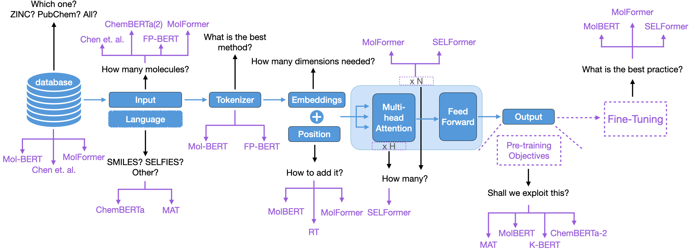
Figure 3: An overview of the individual components of the transformer model and which decisions were explored by which article. Black text represents the set of questions that were asked in the following subsections.

4.1 Which database to use for pre-training, and how many molecules should it contain?

The goal of the pre-training data set is to provide a generic representation of the molecules without the need for labeled information. On the one hand, it has been shown for NLP that selecting the most appropriate data set in terms of diversity or relatedness to the downstream tasks can help the model with faster and better learning and less carbon footprint ¹⁰⁴. On the other hand, the current trend in NLP, for models like GPT, is moving toward increasing the data set size as much as possible ⁵⁴. In addition, several studies suggest that the needed data set size depends on the number of parameters used ^{105, 106}. In this section, we examine how the current chemical language models approached both the data set selection and size for their models.

Molecular databases (see Section 3.1) are assembled and curated for different purposes. The contained molecules can differ and represent different chemical spaces. Table 4 lists transformers from the literature with the databases they were pre-trained on. Some approaches combined molecules from different databases and actively compared the influence of different data sources on prediction performance.

Model Name Pre-training data set Language Database Size ($\sim$) ST ⁶⁰ ChEMBL 900K SMILES RT ⁷⁰ ChEMBL 1.4M SELFIES MolBERT ⁴⁰ ChEMBL (GuacaMol) 1.6M SMILES Transformer-CNN ⁶¹ ChEMBL 1.8M SMILES K-BERT ⁶⁶ ChEMBL 1.8M SMILES SELFormer ⁶⁹ ChEMBL 2M SELFIES ChemBERTa ³⁹ PubChem 100K, 250K, 1M, 10M SMILES, SELFIES ChemBERTa-2 ⁶⁸ PubChem 5M, 10M, 77M SMILES MAT ⁶³ ZINC 2M List of atoms SMILES-BERT ³⁸ ZINC 19M SMILES ChemFormer ⁴¹ ZINC 100M SMILES X-Mol ⁶² ZINC 1.1B SMILES Mol-BERT ⁶⁴ ZINC + ChEMBL 4M Circular FPs MolFormer ⁴² ZINC + PubChem 1.1B SMILES Chen et al. ⁶⁵ C, CP, and CPZ 2M, 103M, 775M SMILES FP-BERT ⁶⁷ E15 2M, 10M Circular FPs

Table 4: The database and the number of molecules used for pre-training each transformer model. The "Database" column shows the source of the pre-training data set. The "Size" column shows the approximate number of molecules used for training each model. The "Language" column shows the molecular representation language used by the corresponding model. FP = Fingerprints, it’s Morgan fingerprints for Mol-BERT ⁶⁴ and ECFP4 for FP-BERT ⁶⁷. C = ChEMBL, CP = ChEMBL + PubChem, and CPZ = ChEMBL + PubChem + ZINC.

Chen et al. ⁶⁵ trained three models with different pre-trained data set combinations, namely, ChEMBL (C), ChEMBL + PubChem (CP), and ChEMBL + PubChem + ZINC (CPZ), containing roughly 2, 103, and 775 million compounds, respectively. The reported performance on five regression data sets for the three models is comparable, i.e., average performance values with overlapping standard errors. For example, for ESOL, an $R^{2}$ of $0.925\pm 0.01$, $0.917\pm 0.012$, and $0.915\pm 0.01$ were reported for C, CP, and CPZ models, respectively. A slightly higher performance trend can be observed for the model pre-trained with only the smaller ChEMBL data set. MolFormer ⁴² was also trained on a combination of two databases, PubChem and ZINC, containing a total of 1.1 billion molecules. The authors reported performance on four additional models trained with weighted combinations of both databases, namely, $10\%$ ZINC + $10\%$ PubChem ($\sim 100$ M molecules), $10\%$ ZINC + $100\%$ PubChem ($\sim 210$ M molecules), and $100\%$ ZINC ($\sim 1$ B molecules). Figure 4(A) shows that the model trained with the smaller data set ($10\%$ ZINC + $10\%$ PubChem) is performing very close to the model trained with ten times the pre-training data set size on the different downstream data sets. For both models, average ROC-AUC values of $\sim 0.85$ were reported for the six classification tasks. In comparison, for three regression tasks, the models trained on the larger data set slightly outperformed those with a smaller data set, with RMSE values of $\sim 0.35$ and $0.37$, respectively. Moreover, the model trained with the second largest data set (100% ZINC) performed worst for the examined downstream data sets (the average difference in ROC-AUC and RMSE is $\sim 0.04$ and $\sim 0.03$, respectively). Figure 4 also shows that the lower performance by training solely on ZINC was not observed when combining only $10\%$ of ZINC with $10\%$ of PubChem. The authors explained the difference in performance by the low vocabulary size and short sequence length of ZINC compared to the other data set combinations.

Other models like ChemBERTa ³⁹, ChemBERTa-2 ⁶⁸, and FP-BERT ⁶⁷ conducted dedicated experiments to analyze the pre-training data set size. ChemBERTa ³⁹ trains four models with 100K, 250K, 1M, and 10M molecules from PubChem. They observe that the increase in performance from training on 100K molecules to 10M molecules for three classification tasks is $\sim 0.11$ ROC-AUC and $\sim 0.06$ PRC-AUC on average. ChemBERTa-2 ⁶⁸, however, does not come to the same conclusion as shown in figure 4(B). The authors also trained three models with 5M, 10M, and 7M molecules from PubChem. Additionally, two models were trained using different pre-training objectives, MLM and MTR. Figure 4(B) shows that increasing the data set size does not always correspond to increased performance for the tested classification tasks. For example, the model trained on the smallest data set using the MLM objective performs almost the same as the model trained on the largest data set for BBBP ($\sim 0.70$ ROC-AUC). In contrast, the same model trained on 5M molecules performs $\sim 0.01$ ROC-AUC better than the model trained on 77M molecules when using the MTR objective. Finally, the FP-BERT ⁶⁷ model trained on 10M molecules showed an increase in ROC-AUC of $\sim 0.01$ and $\sim 0.02$ for BBBP and HIV data sets, respectively, compared to the model trained on 2M molecules from the E15 data set. However, the same trend did not hold for regression as the model trained on 10M molecules from the same data set performed almost the same as the model trained on 2M molecules for ESOL and FreeSolv ($\sim 0.67$ and $\sim 1.1$ RMSE, respectively, for both models), while the model trained on the smaller data set performed $\sim 0.01$ RMSE better for Lipophilicity.

Drawing a clear conclusion from the provided data is difficult. The data set selection and size need further systematic analysis to assess the benefit of scaling. Such systematic analysis has been performed in NLP in publications like Kaplan et al. ¹⁰⁵ and Hoffmann et al. ¹⁰⁶. It would be beneficial to perform a similar analysis for molecular language models. Additionally, the selection of the data set can also affect the performance when the chosen data set does not cover enough chemical space for the downstream data sets, as seen in the model trained on ZINC in MolFormer ⁴². A systematic analysis of the impact of pre-training data set selection can be made by ensuring similarity to desired downstream data sets or by ensuring diversity within the pre-training data set itself ¹⁰⁴.

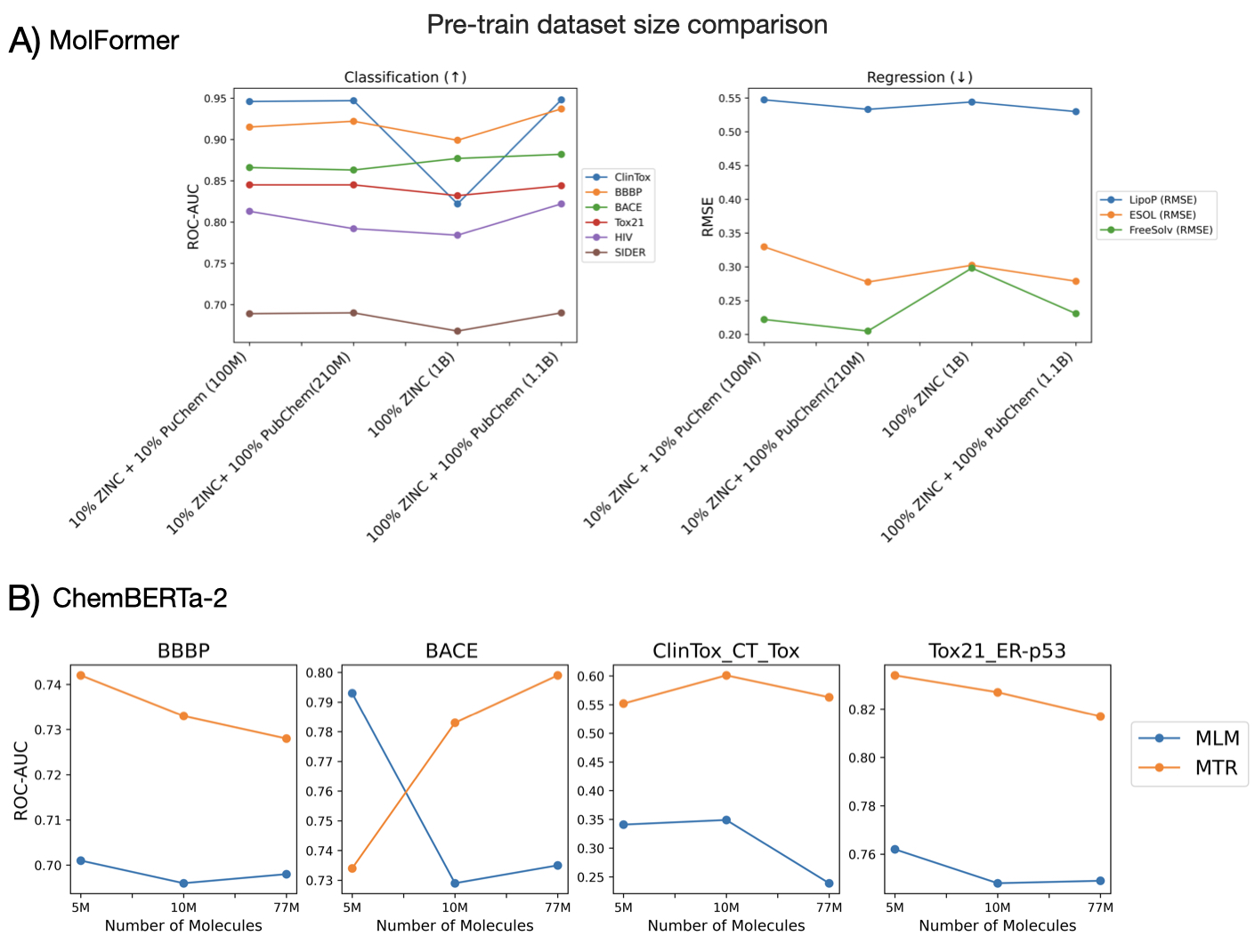
Figure 4: Comparison between the performance and pre-training data set size by A) MolFormer ⁴² and B) ChemBERTa-2 ⁶⁸. The models are sorted in ascending order based on the size of the pre-training data set. ^∗ MLM = Masked language modeling. MTR = Multi-task regression. Data and code used to generate this figure can be found in our GitHub repo.

4.2 Which chemical language to use?

The transformer model is a sequence-based model that relies on learning relations within or between sequences. While molecules are 3D objects, they can be represented as graphs with atoms as nodes and bonds as edges. This molecular graph can be transcribed to produce a 1D representation, i.e., a sequence of atoms and bonds between them. The most common sequence-based small molecule languages are SMILES ²¹ and SELFIES ¹⁰⁷. The majority of the existing models have been trained exclusively using the SMILES representation (Table 4), except for ChemBERTa ³⁹, RT ⁷⁰, SELFormer ⁶⁹, and MAT ⁶³.

The authors of ChemBERTa studied the impact of the choice of chemical language, i.e., SMILES vs. SELFIES, on performance when predicting binding to the stress response target p53 (SR-p53), a task from the Tox21 data set. They concluded that the difference was not significant (without showing further details). For RT, given that the model was designed as a decoder that relies on generation, the authors opted for the SELFIES representation as it is designed to be used in DL generation tasks to produce valid molecules in terms of syntax and properties ^{107, 108}. However, the authors made an initial comparison by training a base model with either SMILES or SELFIES and evaluated both of them for drug-likeness prediction. The results showed very close performance when reporting the RMSE metric. The models trained with SELFIES performed $\sim 0.004\pm 0.01$ better on average. However, reporting the Pearson correlation coefficient metric reverses the conclusion with the SMILES model performing $\sim 0.004\pm 0.01$ better on average. Furthermore, the authors of SELFormer hypothesized that the validity of the SELFIES language makes it more suitable for representation learning than SMILES. The authors compared their model - trained on SELFIES - to the reported values of MolBERT ⁴⁰ and ChemBERTa-2 ⁶⁸ - trained on SMILES. SELFormer performed, e.g., better on the BBBP data set. However, as stated earlier, the need for more standardization of the data splitting makes comparisons inconclusive.

Besides the SMILES vs. SELFIES question, Mol-BERT ⁶⁴ and FP-BERT ⁶⁷ opted for a different input representation. Instead of feeding the molecule to the model as an alphanumeric sequence, the authors exploited circular fingerprints like Morgan fingerprints and ECFP4 to be the input to the model. Both papers used a radius of one to convert the molecular graph into individual atoms and their first-degree neighborhood. The extracted substructures were then hashed and sorted by the atoms’ order in the graph to form a sequence input for the model. FP-BERT ⁶⁷ compared their model to the reported values from MolBERT ⁴⁰. However, as stated earlier, the lack of standardization of the data splitting makes cross-comparisons inconclusive. The Mol-BERT ⁶⁴ model performed a comparison analysis to the SMILES-BERT ³⁸ model on the BBBP, Tox21, SIDER, and ClinTox data sets. Figure 5 A) shows that Mol-BERT outperforms SMILES-BERT on the SIDER data set with no overlapping error bars ($\sim 0.60\pm 0.01$ and $\sim 0.67\pm 0.07$, respectively). It also performs better than SMILES-BERT with minimal overlap in the error bar for Tox21 and ClinTox.

MAT ⁶³ is a model that modified the representation of a molecule by using only the list of its atoms without further grammatical rules as presented in SMILES or SELFIES. However, the authors integrate information about the inter-atomic 3D distances and adjacency in the molecular graph during self-attention calculation. The authors performed a comparison analysis with the ST ⁶⁰ model. Figure 5 (B) shows that MAT performed better than ST on the three compared data sets, $\sim 0.737\pm 0.009$ and $\sim 0.717\pm 0.008$ ROC-AUC, respectively for BBBP, $\sim 0.278\pm 0.020$ and $\sim 0.356\pm 0.017$ RMSE, respectively for ESOL, and $\sim 0.265\pm 0.042$ and $\sim 0.393\pm 0.032$ RMSE, respectively for FreeSolv.

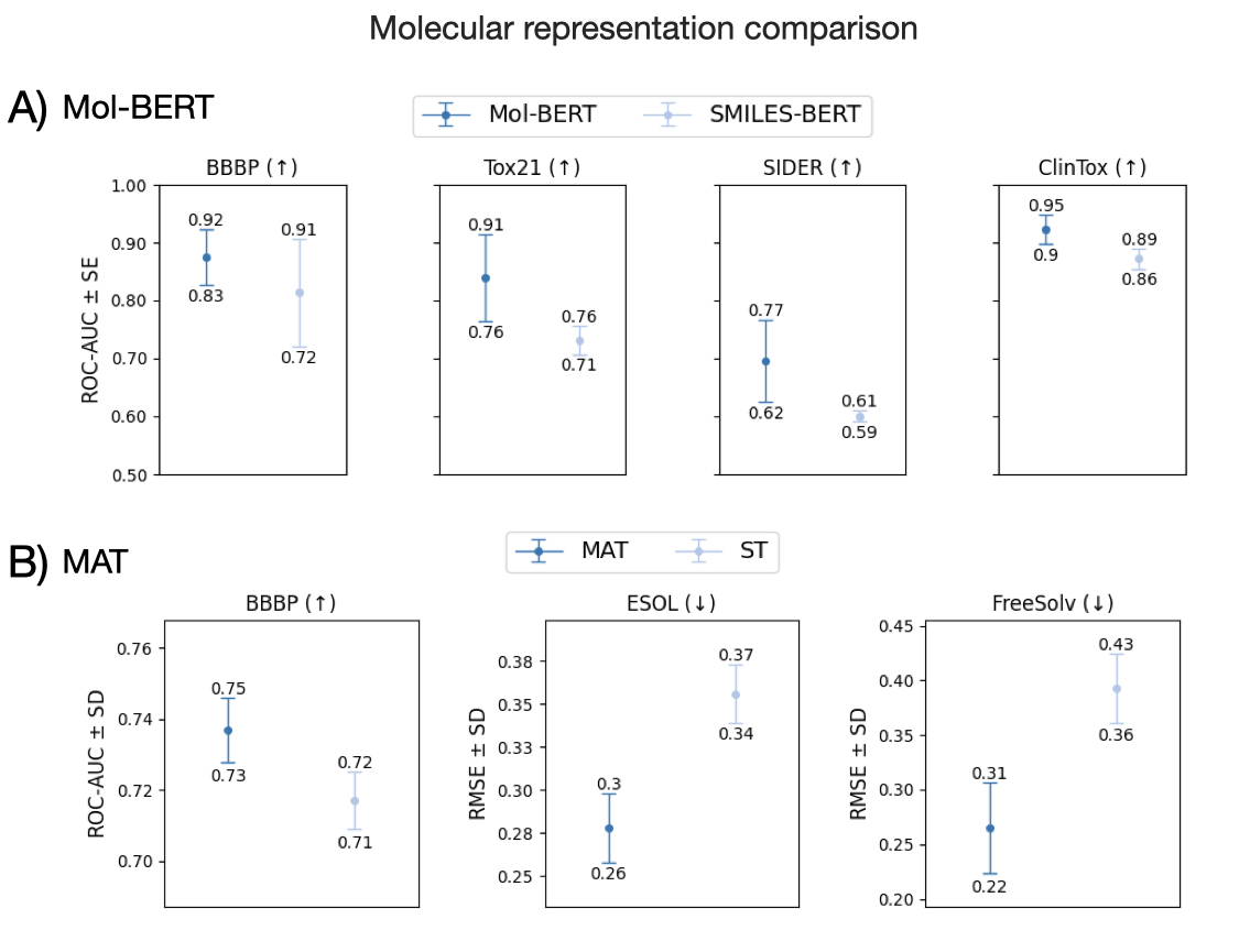
Figure 5: Comparison between the performance of the string-based models and models that used different representation inputs. A) A comparison between the Mol-BERT ⁶⁴ model trained on Morgan fingerprints of radius one and SMILES-BERT ³⁸ trained on SMILES. B) A comparison between the MAT ⁶³ model trained on a list of atoms and SMILES-Transformer (ST) ⁶⁰ trained on SMILES. The figure shows the average performance for each model with error bars (SE) or standard deviation (SD). The data and code used to generate this figure can be found in our GitHub repo.

In conclusion, most of the models have used SMILES for training. Only a few direct comparisons were performed when using SMILES vs SELFIES, for which no significant difference in performance was observed. The choice of the chemical language might depend on the application scenario of the model. For example, RT ⁷⁰ opted for SELFIES as the latter should be more suitable for generative models due to its ensured validity ¹⁰⁷. However, both ChemFormer ⁴¹ and X-Mol ⁶² adopted a decoder subunit while training on the SMILES language, and both reported almost 100% valid molecules for molecular optimization tasks. These results suggest that the transformer model can encode meaningful information from either SMILES or SELFIES. Additionally, using a representation input that ignores syntax, such as in MAT ⁶³, or a different representation as in Mol-BERT ⁶⁴, was performing competitively to the SMILES-based models.

4.3 How to tokenize the molecules?

The transformer model learns an embedding for each token in an input sequence. Different tokenization methods can give a different granularity when representing the composing units of a language. The most popular tokenization schemes in NLP are character-level, subword-level, and word-level ¹⁰⁹. BERT ⁴⁶ and RoBERTa ⁵⁷ adopt similar techniques of subword tokenization where input is firstly tokenized by character. Then, the most common pairs of tokens keep getting merged until reaching a pre-defined vocabulary size. By doing so, a newly observed word during evaluation that is out of vocabulary (OOV) can be tokenized and embedded in terms of its composing subwords.

Model	Tokenizer	Max Vocab	Max Sequence	Positional
Name		Size	Length	Encoding
SMILES-BERT 38	Atom	NA	NA	Absolute
ST 60	Atom	None(1)	220(1)	Absolute (2)
MAT 63	Atom	NA	NA	Absolute (2)
Chen et al. 65	Atom	61 (3)	256	Absolute (2)
Transformer-CNN 61	Atom	66	110	Absolute (1)
MolBERT 40	Atom	42	128	Relative
K-BERT 66	Regex	47	201	Absolute (2)
X-Mol 62	Regex	112(1)	512(1)	Absolute (2)
ChemFormer 41	Regex	523	512(1)	Absolute (2)
MolFormer 42	Regex	2,362	202	Rotary
FP-BERT 67	Substructures	3357	256	Absolute (2)
Mol-BERT 64	Substructures	13,325	200(1)	Absolute (1)
RT 70	Internal Tokenizer	509	250	Relative
SELFormer 69	BPE	800(1)	128(1)	Absolute (2)
ChemBERTa 39	BPE, regex	52K	512	Absolute (2)
ChemBERTa-2 68	Common characters	591	NA	Absolute (2)

Table 5: An overview of tokenization methods and positional encoding by the different models. The "Tokenizer" column specifies how a sequence was split into tokens. The "Max Vocab Column" shows how many unique tokens were selected for the training. The "Max Sequence Length column" specifies the number of tokens in a sequence to be given as input to the model. The "Positional Encoding" column shows how information about the tokens’ positions was added to the model. NA values mean that the authors did not mention it explicitly, did not share the code, or did not provide the code to replicate the results. Footnotes: ¹ This info was not mentioned explicitly in the paper and was derived from the provided code. More information is found in our GitHub repo. ² This information was not mentioned explicitly and is assumed to be the same as the base model mentioned in Table 1. ³ The authors mention 51 in the manuscript, but the supplementary table they refer to shows and counts 61 symbols

Table 5 shows which tokenizer was used for each reviewed model and the maximum number of tokens in the used vocabulary. Different tokenizers have been utilized for the SMILES language, such as the atom-level tokenizer, where the sequence is split into its composing atoms, numbers, and special characters. The regular expression (regex) tokenization was proposed by Schwaller et al. ¹¹⁰, which also segments the molecule into individual atoms. However, the characters within a square bracket and the double digits preceded by % are treated as single characters. ChemBERTa ³⁹ and SELFormer ⁶⁹ utilized the byte-pair encoder (BPE) used in RoBERTa ⁵⁷, which performs subword tokenization. Moreover, ChemBERTa ³⁹ attempted a comparison between the BPE and the regex tokenizers on the SR-p53 task of the Tox21 data set, where an improvement of 0.015 PRC-AUC for the regex tokenizer was reported. The RT ⁷⁰ model used the SELFIES internal tokenizer, which splits the molecule based on the language-specified symbols ¹⁰⁷. The only models that used a different tokenization method were Mol-BERT ⁶⁴ and FP-BERT ⁶⁷, where the sequence was converted into substructures using circular fingerprints.

The vocabulary size is a trainable parameter that adds to the model’s complexity. Models like BERT ⁴⁶ and RoBERTa ⁵⁷ use vocabularies of sizes around 30K and 50K, respectively. It can be seen that, for the chemical language models, the vocabulary size varied dramatically from as little as 42 tokens for MolBERT ⁴⁰ to over 52K tokens for ChemBERTa ³⁹ (Table 5). None of the articles provided further analysis of the effect of varying the vocabulary size on performance.

In conclusion, there is currently no detailed analysis available on which tokenization method may be most beneficial for which research question. However, it should be relevant to experiment with meaningful multi-character tokenizations as this provides the composing units of the sequence that the model will learn to represent ¹⁰⁹. A meaningful tokenization method can also allow us to judge the model’s explainability. One possible approach for tokenization is to extend it to proper and informative fragmentation of the molecules by using methods relying on chemical rules (e.g., molBLOCKS ¹¹¹, eMolFrag ¹¹², etc.) or data-driven methods (e.g., SMILES-base encoder (SPE) ¹¹³, Morfessor ¹¹⁴, etc.).

4.4 How to add positional embeddings?

The transformer ³ models rely on the attention mechanism to calculate the relationships between the tokens. However, this process is known to be position-agnostic ¹¹⁵. Therefore, information about the position of each token needs to be included so that the model can draw position-aware relationships. The original transformer ³ model provides an absolute and fixed positional encoding using different scaled sinusoidal functions. For each position in the sequence, a specific vector of the same length as the token’s embedding is added to the token’s embedding. Other models like GPT ⁵³, BERT ⁴⁶, and RoBERTa ⁵⁷ used a trainable absolute positional embedding so that the model would learn the embeddings of each position instead of having it pre-calculated. Fixed and trainable approaches are constrained by the sequence length when representing the absolute positions. Consequently, the model cannot assign a positional encoding if a longer sequence is encountered during evaluation. Therefore, other models ^{116, 73} have attempted to learn a relative positional encoding, allowing for more flexible sequence processing during evaluation.

Table 5 shows the types of positional embedding used for the reviewed articles. All the models are inferred to use the same positional embedding as their base models, as detailed in Table 1. However, MolBERT ⁴⁰, RT ⁷⁰, and MolFormer ⁴² reported different methods for incorporating positional embedding. MolBERT ⁴⁰ and RT ⁷⁰ adopted a relative positional embedding ¹¹⁶ in which the position of a token is learned based on its position from the surrounding tokens. MolFormer ⁴² opted for positional embeddings that combined both absolute and relative concepts, namely, Rotary Positional Embedding (RoPE) ⁷³. An advantage of the RoPE method is that it is compatible with the memory-efficient linear attention mechanism used in MolFormer ⁴². MolFormer ⁴² performed a comparison between training their models with either absolute positional embedding or RoPE on the QM9 data set. Their preliminary results showed that the absolute embeddings performed better than the out-of-box implementation of RoPE. However, with their modified RoPE implementation, the authors found it to provide better performance when the pre-training data set size became huge. The authors report an average and standard deviation MAE over 13 regression tasks from the QM9 data set for models trained with 111K, 111M, and 1.1B molecules, respectively. The difference in performance between the absolute and RoPE positional embedding for these three models are $\sim-0.20\pm 0.18$, $\sim-0.44\pm 0.22$, and $\sim 0.27\pm 0.12$, respectively. These results demonstrate that the RoPE embeddings were superior to absolute embeddings, but only when the pre-training data set was very large.

An important aspect is that languages like SMILES and SELFIES are linearized versions of the 2D molecular graph. Consequently, two consecutive tokens in sequence are not necessarily nearby in 2D or 3D representation. Therefore, encoding tokens’ 2D or 3D positions might be more beneficial than encoding the positions in a SMILES sequence. The authors of MAT ⁶³ incorporated spatial information such as inter-atomic 3D distances and adjacency in the 2D molecular graphs. They did so by integrating such information alongside the self-attention mechanism. This approach performed comparably (Figure 5 B) to the ST ⁶⁰ model, which uses absolute and fixed positional embeddings based on the SMILES sequence.

In conclusion, most of the papers have utilized the absolute positional embedding of their base model, which is either fixed or trainable, except for MolBERT ⁴⁰, RT ⁷⁰, and MolFormer ⁴². These first analyses indicate that changing the absolute embedding helped when the pre-training data set was very large ⁴². Moreover, attention needs to be paid to how positional embeddings are used. Since molecules exist in 3D space, it can be challenging for linear chemical languages to fully represent the nature of molecules. For example, the SMILES representation is a linearization of the 2D molecular graph. Consequently, a positional embedding that accounts for the actual location of each token in 2D (the molecular graph) or 3D space would be an interesting direction to explore.

4.5 How many parameters do we need?

The transformer architecture consists of multiple parameters that need to be set and optimized for the underlying problem. For example, the transformed embeddings can be split between multiple attention heads inside an encoder or a decoder layer. By doing so, each head can attend separately to different dimensions of the tokens. Moreover, multiple transformer layers can be stacked to increase the depth of learning as each layer passes its learned representation of the tokens’ embeddings to the next layer. Another parameter is the embedding length (usually referred to as the hidden size), as increasing it might correspond to higher expressiveness and generalization capabilities. The number of layers and the embedding length account for the total number of parameters to be learned by the model. Additionally, another set of parameters is encountered when learning the input embeddings to the model, which depends on the embedding length and the vocabulary size. The current trend in NLP has been towards increasing the number of parameters to allow for higher-quality learning by the model. For example, BERT ⁴⁶ was trained as a small model with 110M parameters and a large model with 230M parameters. The RoBERTa model was trained on 335M parameters, while GPT2 ⁵⁴ and GPT3 ⁵⁴ models were trained with 1.5B and 175B parameters, respectively.

Table 6 shows that most of the chemical language models applied for MPP were trained with $\leq$ 100M learnable parameters, which is in the small range of model sizes compared to models from NLP. The small size of the chemical language models might be understandable since languages like SMILES contain much smaller vocabulary and grammatical rules than natural languages. The table also shows how the choices of the individual hyperparameters varied between the different models. For example, ST ⁶⁰ embedded their tokens with 256 dimensions, while SMILES-BERT ³⁸ and MAT ⁶³ used 1024 dimensions for the embeddings. The number of layers varied from 4 to 32 by ST ³⁸ and MAT ⁶³, respectively.

Model Name # dimensions # head # layer # parameters ($\sim$)(¹) Model Embeddings ST ⁶⁰ 256 4 4 7M NA Mol-BERT ⁶⁴ 300 6 6 7M 4M Transformer-CNN ⁶¹ 512 10 3 22M 34K Chen et al. ⁶⁵ 512 8 8 25M 26K RT ⁷⁰ 256 16 32 25M 130K K-BERT ⁶⁶ 768 12 6 43M 36K ChemBERTa-2 ⁶⁸(²) 768 12 6 43M 454K ChemBERTa ³⁹ 768 12 6 43M 40M ChemFormer ⁴¹ 512 8 6 44M 268K SMILES-BERT ³⁸ 1024 4 6 76M NA MolBERT ⁴⁰ 768 12 12 85M 32K X-Mol ⁶² 768 12 12 85M 86K MolFormer ⁴² 768 12 6, 12 43M, 85M 2M, 2M SELFormer ⁶⁹ 768 12, 4 8, 12 57M, 85M 614K, 614K MAT ⁶³ 1024 16 8 101M NA FP-BERT ⁶⁷ 256 NA NA NA NA

Table 6: Some of the architecture choices for training the transformer blocks. The "# dimensions" table corresponds to the embedding dimensions (also known as hidden size). The "# head" corresponds to the number of heads specified per each attention block. The "# layers" specifies the number of stacked encoders/decoders. The "# parameters" corresponds to the number of learnable parameters by the models. NA values mean that the authors did not mention it explicitly and either did not share the code or did not provide the code to replicate the results. Footnotes: ¹ These values were calculated based on the provided information. The model’s parameters depend on the model dimensions (hidden size) and the number of layers, while the embedding parameters depend on the vocabulary and hidden sizes. A script that does and explains the calculations can be found in our GitHub repo. ² ChemBERTa-2 ⁶⁸ did not mention the corresponding parameters explicitly and were assumed to have the same parameters as ChemBERTa ³⁹.

As shown in Table 6, only MolFormer ⁴² and SELFormer ⁶⁹ provided MPP analysis for different sizes of their models. SELFormer ⁶⁹ varied the number of heads and the number of layers jointly and reported the performance on different classification and regression data sets. When fine-tuning both models using 50 epochs, the large model with $\sim 86M$ parameters performed better for some data sets (e.g., $\sim 0.034$ $\triangle ROC-AUC$ for BBBP) and very comparably for others (e.g., $\sim 0.001$ $\triangle ROC-AUC$ for BACE) A similar trend was observed for regression as the larger model performed $\sim 0.013$ $\triangle RMSE$ better for FreeSolv, while the improvement was only $\sim 0.007$ for PDBind. However, the smaller model could perform $\sim 0.013$ better for LipoPhilicity. The previous observation shows that a larger model can improve the performance compared to a smaller model, which was also observed for most of the data sets for the MolFormer ⁴² model. The larger model with $\sim 87M$ parameters performed $\sim 0.04$ ROC-AUC better on average than the smaller model ($\sim 57M$ parameters) for BBBP, HIV, BACE, and SIDER data sets. The larger model also performed better on FreeSolv ($\sim 0.12$ $\triangle RMSE$) and very comparably on ESOL ($\sim 0.001$ $\triangle RMSE$). The exception to the previous trend was noticed in the ClinTox and Tox21 data sets, as the larger model prominently outperformed the smaller model with as much as 0.34 and 0.42 ROC-AUC, respectively.

In conclusion, the current state-of-the-art does not allow for systematical analysis of parameter scaling in transformer models for MPP. Preliminary analysis shows that larger models can provide some improvement. However, publications from the NLP domain show that scaling the model’s parameters (aka, model size) should be carried out alongside the scaling of the training data set size ^{105, 106}. Additionally, Kaplan et al. ¹⁰⁵ concluded that such scaling is more sensitive to the model size irrespective of the model shape (e.g., different models with the same number of parameters but different embedding lengths and the number of layers should behave similarly). However, Tay et al. ¹¹⁷ argue that model shape and size contribute to efficient downstream transfer. Therefore, proper systematic analysis of model scaling, similar to NLP, is still needed for the chemical language models to identify the most efficient choices.

4.6 Which pre-training objectives to adopt?

The transformer ³ models rely on self-supervised learning. Models developed with this scheme learn from labels that can be easily created from unlabeled data. Table 7 shows the objectives used for each reviewed article, which can be grouped into domain-agnostic and domain-specific. Most models used the same objectives as their base transformer model, originally built for NLP. Therefore, the objective is independent of the application area. However, models like MAT ⁶³, MolBERT ⁴⁰, K-BERT ⁶⁶, and ChemBERTa-2 ⁶⁸ used objectives that are specific to the chemical languages and general chemical information, hence, introducing inductive bias.

MAT ⁶³ used the interatomic 3D distances and the adjacency matrix of the molecular graph to integrate them as additional sources of information alongside the self-attention mechanism. In the ablation analysis, the authors removed one source of information at a time. They reported performance on BBBP, ESOL, and FreeSolv data sets as shown in Figure 6. The data sets behaved differently for each model. For example, the most stable performance for ESOL in terms of standard deviation was the model without the interatomic distance ( $\sim 0.28\pm 0.001$ RMSE). However, the model trained with the three objectives was the most stable across the three data sets.

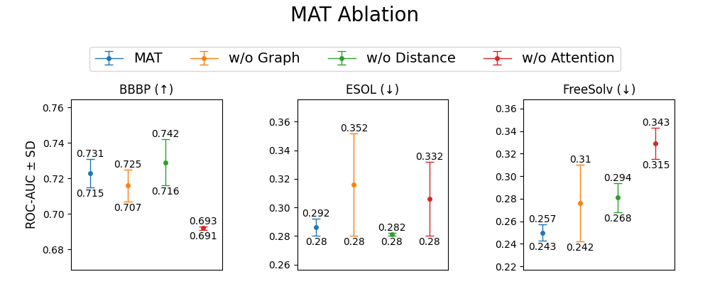
Figure 6: The ablation analysis by the MAT model⁶³. MAT = the model trained with the three sources of information, self-attention, interatomic 3D distances, and adjacency matrix. w/o graph = the MAT model trained with self-attention and interatomic distances only. w/o Distance = the MAT model with self-attention and adjacency only. w/o attention = the MAT model with interatomic distances and adjacency only. The data and code used to generate this figure can be found in our GitHub repo.

MolBERT ⁴⁰ introduced two new objectives alongside MLM: PhysChemPred and SMILES-EQ. The former objective entails training the model to predict $\sim$ 200 physico-chemical properties. At the same time, the latter classifies a pair of SMILES as equivalent or not, given the non-uniqueness feature of the SMILES language. In their analysis of virtual screening outcomes, the authors found that the PhysChemPred objective performed very closely to the model trained with the three objectives, $\sim 0.72\pm 0.06$ and $\sim 0.71\pm 0.06$ ROC-AUC, respectively (Supplementary Figure 8). ChemBERTa-2 ⁶⁸ incorporated the same PhysChemPred objective, naming it Multiple Task Regression (MTR), and compared its performance to a model trained with MLM only. Figure 4 (B) shows that the model trained with MTR-only performed noticeably better for almost all four classification tasks and pre-training data set size combinations than MLM-only. The SMILES-EQ objective proposed by MolBERT ⁴⁰ was found to lower the performance when combined with the other objectives, $\sim 0.71\pm 0.06$ and $\sim 0.74\pm 0.07$ ROC-AUC for the models with and without the SMILES-EQ objective, respectively. However, K-BERT ⁶⁶ incorporated the non-uniqueness of the SMILES language as well but as a contrastive learning (CL) objective. With this objective, the model is trained to maximize the similarity between the SMILES sequences of the same molecule while minimizing similarities to the other sequences. In their ablation analysis, the model trained with and without CL performed similarly for the 15 tested data sets (Supplementary Figure 9) with an average ROC-AUC of $0.806$ and $0.807$, respectively. The authors used two other objectives: predicting features of heavy atoms (e.g., hybridization) and the molecule’s MACCS keys descriptor. However, no further ablation analysis was performed for these two objectives.

In conclusion, most models utilized the domain-agnostic pre-training objectives as their base transformer model. The remaining models that used inductive bias showed it can boost performance. This line of research might be interesting since chemical languages like SMILES are not self-contained, but other factors influence molecular properties. Thus, further physico-chemical properties or 3D conformations might be needed to improve the prediction performance of individual properties. Additionally, it would be interesting to quantify the extent of what the language model captures independently to understand better which objectives would further enhance the model’s performance and explainability. For example, visualizing the attention scores calculated for the tokens during training and fine-tuning can help to understand what the model is paying attention to and whether it is relevant to the downstream data set ¹¹⁸. Payne et al. ¹¹⁹ performed such an analysis by training a BERT-based model to quantify the model’s ability to capture functional groups. They visualized the attention scores and leveraged chemical knowledge to judge whether the model paid proper attention to well-described functional groups.

Model Name	Pre-training objective (1)	Fine-tuning
X-Mol 62	-	Update
ST 60	-	Frozen
FP-BERT 67	MLM	Frozen
MolFormer 42	MLM	Frozen, Update
SELFormer 69	MLM	Frozen, Update
SMILES-BERT 38	MLM	Update
ChemBERTa 39	MLM	Update
Mol-BERT 64	MLM	Update
Chen et al. 65	MLM (Guided)	Update
RT(2) 70	PLM	-
Transformer-CNN 61	Augmentation	Update
ChemFormer 41	Denoising Span MLM, Augmentation	Update
MAT 63	MLM, 2D Adjacency, 3D Distance	Update
MolBERT 40	MLM, PhysChemPred, SMILES-EQ	Frozen, Update
ChemBERTa-2 68	MLM, MTR	Update
K-BERT 66	Atom feature prediction, MACCS prediction, CL	Update last layer

Table 7: A list of the pre-training objectives and the fine-tuning choices made by the reviewed articles. Footnotes: ¹ MLM = Masked Language Modelling. Guided MLM refers to masking chemically relevant tokens (e.g., functional groups). PLM = Permutation Language Modelling. PhysChemPred = Physico-chemical properties prediction for a molecule. SMILES-EQ = SMILES equivalence, identifying whether two SMILES represent the same molecule. CL = Contrastive learning, the task of learning representations by contrasting positive and negative samples. MTR = Multiple Task Regression (same as PhysChemPred). ² Regression Transformer was trained with the aim of performing multi-task learning during pre-training. Therefore, they did not perform fine-tuning.

4.7 How to fine-tune?

After optimizing the model’s architecture and training on large unlabelled data sets, it can be used for a wide range of downstream tasks. Therefore, a pre-trained model can be a generic basis for multiple applications. The output representation of the model can be used directly as a proper numeric descriptor, a so-called embedding, of the input ¹²⁰. When the downstream data set is closely related to the pre-training data, the output representation can be used as the input for a classifier/regressor model for the said data set. In this scenario, the model’s weights are frozen and do not go through any further updating phase ^{120, 121}. The other method of fine-tuning is to update the weights by appending a classification/regression neural network head to predict the output of the underlying downstream data set ^{120, 121}. In this scenario, one or more of the model’s layers get updated to maximize the performance gain on the corresponding labeled data set. Updating the weights requires further hyperparameter tuning to find the best learning convergence ¹²¹. The full model update has been used in many publications ^{3, 46}. However, this causes further computational toll. Some methods from NLP have been proposed to enable efficient fine-tuning by updating specific relevant weights or biases or even updating a small initialized new weight matrix and adding it to the frozen original model ¹²¹.

Table 7 shows the different fine-tuning methods used by the discussed models. ST ¹¹³ and FP-BERT ⁶⁷ were the only two models that used the frozen fine-tuning strategy alone, while the rest used either the update strategy only or compared the performance of both. We assume the full model updating was performed for the updating strategy since no contradicting information is provided in the manuscripts. Only K-BERT ⁶⁶ stated that they updated the weights of the last layer of the model. MolBert ⁴⁰ and SELFormer ⁶⁹ compared their models using the two strategies on multiple downstream data sets, while MolFormer ⁴² tested the two strategies on the QM9 data set only. Tabel 8 shows the difference in performance between frozen and updated models of MolBERT ⁴⁰ and SELFormer ⁶⁹ for three regression data sets. The table shows that updated models performed better than the frozen model (e.g., a difference in the performance of 0.575 and 2.187 $\triangle RMSE$ for MolBERT and SELFormer, respectively, for the FreeSolv data set). However, the SELFormer ⁶⁹ model seems to benefit from weight updates much more than MolBERT ⁴⁰ for the three shown data sets in table 8. This observation might be explained by the pre-training objectives used in MolBERT that might have improved the learned representations before fine-tuning. For example, Payne et al. ¹¹⁹ show that a certain layer in the fine-tuned model on the solubility data set has learned to attend to the long carbon chain in the molecule. This observation relates well with the LogP (partition coefficient), which indicates the relationship between lipophilicity and solubility. The pre-training objectives in MolBERT ⁴⁰ included physico-chemical properties, such as LogP, making the pre-trained model closer to some downstream data sets. Another observation from Table 8 is that SELFormer Lite, which is a smaller version of SELFormer in terms of the model’s parameters, is seen to benefit from weight updates fine-tuning more than the larger model for ESOL (1.311 and 0.871 $\triangle RMSE$, respectively).

In conclusion, fine-tuning can be done in multiple ways ¹²¹, where the current literature investigated a couple of approaches. The analysis shows that fine-tuning through weight updates provides better performance than frozen weights, which is understandable since fine-tuning by weight updates further directs the model to output embeddings that are more related to the downstream task. Additionally, domain-specific pre-training objectives and architectural choices, such as the number of parameters, can also influence the performance of the fine-tuned model.

	$\triangle$ (Frozen - Updated) RMSE
	ESOL	FreeSolv	Lipophilicity
MolBERT 40	0.021	0.575	0.041
SELFormer 69	0.971	2.187	0.310
SELFormer Lite 69	1.311	2.112	0.388

Table 8: The advantage of fine-tuning through weight updates vs frozen weights. SELFormer and SELFormer Lite differ in the number of parameters. Random split was used for the three datasets by both models. The weight update strategy provides better results. However, some models seem to benefit more from this strategy than others. The results were reported for regression only as SELFormer compared fine-tuning strategies using random split while MolBERT used scaffold split.

5 Current challenges for MPP with transformers

In this review, we collected and assessed the performance of the currently ubiquitous transformer models for molecular property prediction. By categorizing the approaches and ideas from the literature, we found varying handling of benchmark data sets and reporting transparency to be the main obstacles.

We observed that different test sets are often used by different publications (see Section 3.3), which makes proper comparison of different models infeasible due to the lack of standardization. Firstly, not all models adhered to the recommended scaffold split for the data sets, which is supposed to test the model’s generalizability better than a random split. Secondly, many papers used different splitting modules with different random seeds and sometimes various split ratios. Thus, each model was tested on a different test set, precluding proper comparison. Therefore, it is absolutely crucial to have a unified test split for the recommended splitting method so that benchmarking new and old models becomes accessible and more meaningful.

Given the broad collection of labeled property data sets (see Section 3.2), selecting the most relevant ones is difficult. For example, the commonly used data sets from MoleculeNet or TDC and their experimental property data are heterogeneous. The data set sizes and compositions differ and might represent the respective endpoints in varying quality and generality. For example, contained molecules might cover only a limited chemical space, the property distribution is narrow or does not cover the practically relevant range. In addition, other relevant molecular properties are not covered, e.g., because of a lack of data or expensive manual curation for raw data processing. This can make benchmark collections not sufficiently represent real-world scenarios and inadequately describe the practical usefulness of prediction models. We believe that a high-quality description of the downstream tasks would help to focus and foster method development in the future.

In this direction, some studies propose more detailed and systematic comparisons of molecular representations ^{122, 9}. They focus on the well-known concepts of molecular scaffolds and "activity cliffs" and describe frameworks to analyze and identify desired representations for MPP. A good representation should be able to generalize across structurally different molecules (called "generalized scaffold hopping" ¹²² and "inter-scaffold generalization" ⁹) and be able to accurately represent small structural molecule modifications which result in considerable property changes (referred to as "generalized activity cliffs" ¹²² and "intra-scaffold generalization" ⁹). There are already benchmark platforms dedicated to activity cliffs, like MoleculeACE ¹²³.

We enlisted a set of questions in this review that we believe are important for designing an efficient transformer model for MPP (see Section 4). However, extracting the relevant information from each article was not always easy. Moreover, fishing for the needed information from the provided code by some articles was also very challenging. We believe the list of questions we provide in this review is a good start for agreeing on what should be reported in future works to enable meaningful comparisons and meta-analysis. We also believe that providing a structured and well-documented code repository for the community would help navigate the code and extract further useful information.

We almost found a consensus on model evaluation metrics between the articles, as most used ROC-AUC for classification and RMSE or MAE for regression (see Section 3.3). These metrics were also proposed in the MoleculeNet ⁶ paper as the authors also observed the community using ROC, PRC, RMSE, and MAE. They further vouched for the selection of ROC or PRC based on the severity of class imbalance for classification data sets. For example, PRC-AUC is considered a more suited alternative for strongly imbalanced data sets ^{124, 6}. Although a single metric is easy to compare and draw insights upon, it can hardly capture the complete picture ¹²⁵. Therefore, it might be of interest for the community to consider multiple metrics to provide complementary insights about the performance ¹²⁶.

Further, metric values alone are usually insufficient to comprehensively judge the model’s performance (see Section 3.3). The next step should be performing statistical analysis to emphasize further that a performance improvement is consistent and robust ¹²⁷. Statistical analysis requires multiple and independent runs of the evaluation step and the selection of the most appropriate measure to calculate significance ^{127, 128}. As only a few reviewed articles performed statistical analysis, we believe the community needs proper statistical analysis ¹²⁹ to provide robust and meaningful conclusions.

After a proper evaluation, visualizing performance is crucial to engage the reader and allow other researchers to form an insightful understanding. Most reviewed papers report their findings as a table or bar plot. A table format requires the reader to mentally visualize the performance of the different models, which is challenging. Additionally, a bar plot cannot visualize continuous data as different distributions can correspond to the same bar plot ¹⁰⁰. For multiple evaluation runs, a summary plot like a boxplot will be more engaging and informative than a scatter plot ^{100, 101}. Moreover, plotting each data point is recommended when the number of runs is relatively small, as the summary drawn from a small number of data points might not be representative ¹⁰⁰.

6 Conclusion and outlook

This work reviews the articles that trained a sequence-based transformer model for molecular property prediction (MPP). Our analysis showed that the transformer models have not unleashed unprecedented performance as seen in other fields like NLP ³ (Figure 7). However, they have shown promising performance compared to the existing MPP models. In an attempt to identify the factors that might aid in designing better transformer models for MPP, we explored various questions to which we found the following preliminary answers:

• There are large enough data sets of unlabeled molecules that can be used for pre-training, e.g. ChEMBL, PubChem, ZINC, and even public and proprietary fragment spaces ranging up to $10^{26}$ molecules ¹³⁰. However, results indicate that size alone is not the sole determinant of successful downstream predictions, but the data set composition, i.e., the covered chemical space, is equally relevant. Therefore, it is important to determine the relevant factors of pre-training data set composition that help to train predictive and generalizable models efficiently. Future directions might include the clustering and filtering of large databases while maintaining prediction performance on downstream tasks.

• Chemical languages such as SMILES and SELFIES are one way of linearizing the molecular graph while introducing some grammatical rules that add semantic information. Preliminary analysis shows that both languages are similarly sufficient for training a transformer model. Additionally, the input does not need to be strictly limited to these representations as other approaches can also work well when the model’s architecture is adjusted accordingly ^{67, 64, 63}.

• The tokenization of the input sequence is an important step that determines the granularity of the model training. However, different approaches have not yet been systematically compared, and most groups have used character-based tokenization techniques. Future works can investigate the benefit of chemically and biologically meaningful tokenization for the downstream performance and explainability benefit.

• The positional encoding has not undergone intensive analysis. The atoms of a molecule in the molecular graph have different relative positions in the generated SMILES or SELFIES. Therefore, questioning the proper way to incorporate positional embedding that reflects a token’s 2D or 3D position is worth further studies.

• In the NLP field, it has already been studied that model size (number of parameters) should be scaled concurrently with the data size ^{105, 106}. In some of the reviewed articles, scaling the model parameters was performed, but the data set size was fixed. Therefore, systematic analyses, like those in NLP, are needed to understand how the chemical language models behave under these constraints.

• Pre-training objectives like masked language modeling (MLM) are mostly domain-agnostic. Multiple papers explored the effect of incorporating domain-specific objectives and comparisons showed a promising trend. However, some domain-specific objectives can be learned from the domain-agnostic objectives ¹¹⁹. Therefore, further analysis is desirable to identify the needed pre-training objectives.

• Fine-tuning a pre-trained model by weight updates is needed when the downstream data differs considerably from the pre-training data, which can be computationally expensive. Some discussed studies compared the frozen strategy to weight updates and reported the superior performance of the latter. However, we observe that architectural and pre-training choices can affect the added value of this step. Future work is needed to compare different fine-tuning strategies with different models to identify when the expensive step of weight updates is needed and how to perform it most efficiently.

• The literature’s current performance evaluation process lacks important factors that enable proper comparisons. The community must ensure, document, and provide appropriate splitting for the downstream data set and a corresponding fixed test set for each split. Furthermore, statistical and significance analysis is highly needed, which is a vital factor for faithfully judging a model’s benefit.

• Visualization reporting is also one way of engaging the reader and allowing further valuable insights. We believe that reporting needs to move from a simple table to a proper visualization of the different runs and their distribution summary (e.g., boxplots).

• This review focused on architectural and domain-relevant exploration for training a transformer model. Addressing further aspects like weight initialization and selection of hyperparameters for both pre-training and fine-tuning steps would also be helpful for future work.

• Additionally, one of the main advantages of the transformer models is their ability to capture long-range dependencies, which is usually identified through attention visualization of the trained and fine-tuned models ¹¹⁸. Therefore, reviewing the explainability analysis done by the different models can help to identify and highlight the added benefit of the transformer model. It can also help to shed light on the weaknesses that must be addressed to improve the model’s performance further.

• The current literature on chemical language models often focuses on approaches and ideas from natural language processing. The NLP field is moving fast and there are multiple new ideas and applications ¹³¹ that may improve chemical model performance, including pre-training regimes ^{132, 133}, fine-tuning strategies ^{134, 135}, explainability ¹³⁶ and more. At the same time, the requirements for chemical language models differ from those in NLP. For example, chemical models have smaller vocabularies and lower sequence lengths (see Table 5), and not all concepts need to be transferred from text to molecules. Therefore, adapting models to the specificities of chemical data necessary to accurately predict the properties of molecules needs to be explored in the future.

In conclusion, the transformer models show promising performance for molecular property prediction. We believe that they can be further improved when accounting for the identified best practices and recommendations mentioned above. Finally, we believe the transformer’s context-dependent embeddings can improve the intricate association of the molecule’s structure with molecular properties. In addition, the self-supervised learning scheme can potentially improve small labeled tasks. Both characteristics make transformers a promising addition to existing models. Therefore, we believe that further improvements in the transformer model to match the requirements of molecular property prediction will provide better performance, generalizability, and explainability.

The authors thank Soheila Samiee and Jesujoba Oluwadara Alabi for valuable discussions that improved the manuscript.

Model Name BBBP HIV BACE Tox21 ClinTox SIDER Others MolFormer ⁴² - ST ⁶⁰ - - SELFormer ⁶⁹ - - Transformer-CNN ⁶¹ - AMES, JAK3, BioDeg, RP AR. Mol-BERT ⁶⁴ - - - X-Mol ⁶² - - MUV. ChemBERTa ³⁹ - (¹) (¹) - - MolBERT ⁴⁰ - - - - Chen et al. ⁶⁵ - - - AMES, BEET. ChemBERTa-2 ⁶⁸ - - (¹) -(¹) - - FP-BERT ⁶⁷ - - - - - MAT ⁶³ - - - - - ESTROGEN-a, ESTROGEN-ß, METSTABLow, METSTABHIGH. SMILES-BERT ³⁸ - - - - - - LogP, PM2, PCBA 686978. ChemFormer ⁴¹ - - - - - K-BERT ⁶⁶ - - - - - - Pgb-sub, HIA, F(20%), F(30%), FDAMDD, CYP1A2-sub, CYP2C19-sub, CYP2C9-sub, CYP2D6-sub, CYP3A4-sub, T12, DILI, SkinSen, Carcinogenicity, Respiratory, Malaria. RT ⁷⁰ (²) - - - - - - -

Table 9: The classification data sets used by some of the models. These models used scaffold split except for X-Mol, Trnasformer-CNN, and Chen et al. Footnotes: ¹ a single task was predicted for this data set instead of all tasks as done by the other models. ² Regression Transformer (RT) was trained for predicting regression data sets only.

Model Name	ESOL	FreeSolv	Lipophilicity	Others
ST 60				-
MolBERT 40				-
Chen et al. 65				LogS, DPP4.
ChemFormer 41				-
X-Mol 62				-
FP-BERT 67				Malaria, CEP.
MolFormer 42				QM9, QM8.
RT 70				-
SELFormer 69				PDBind.
MAT 63			-	-
Transformer-CNN 61	-			MP, BP, BCF, LogS, BACE, DHFR, LEL.
SMILES-BERT 38	-	-	-	-
ChemBERTa 39	-	-	-	-
Mol-BERT 64	-	-	-	-
K-BERT 66	-	-	-	-
ChemBERTa-2 68	-	-	-	Clearence, Delaney, BACE.

Table 10: The regression data sets modeled by some of the models. These models used random split.

End Point	% Positive	# Molecules
CT_TOX	8.0	1484
FDA_APPROVED	94.0	1484

Table 11: The percentage of positive class per task for the ClinTox data set. FDA_approved corresponds to compounds that have been approved by the FDA. CT_TOX corresponds to compounds that failed in clinical trials due to toxicity reasons. Data and code used to generate this table can be found in our GitHub repo.

End Point % Positive # Molecules Product issues 2.0 1427 Pregnancy, puerperium and perinatal conditions 9.0 1427 Surgical and medical procedures 15.0 1427 Congenital, familial and genetic disorders 18.0 1427 Social circumstances 18.0 1427 Endocrine disorders 23.0 1427 Neoplasms benign, malignant and unspecified (incl cysts and polyps) 26.0 1427 Ear and labyrinth disorders 46.0 1427 Reproductive system and breast disorders 51.0 1427 Hepatobiliary disorders 52.0 1427 Eye disorders 61.0 1427 Blood and lymphatic system disorders 62.0 1427 Renal and urinary disorders 64.0 1427 Injury, poisoning and procedural complications 66.0 1427 Cardiac disorders 69.0 1427 Metabolism and nutrition disorders 70.0 1427 Infections and infestations 70.0 1427 Musculoskeletal and connective tissue disorders 70.0 1427 Psychiatric disorders 71.0 1427 Immune system disorders 72.0 1427 Respiratory, thoracic and mediastinal disorders 74.0 1427 Vascular disorders 78.0 1427 Investigations 81.0 1427 Nervous system disorders 91.0 1427 General disorders and administration site conditions 91.0 1427 Gastrointestinal disorders 91.0 1427 Skin and subcutaneous tissue disorders 92.0 1427

Table 12: The percentage of positive class per task for the SIDER data set. Each row corresponds to compounds that have been affiliated with a certain side effect. Data and code used to generate this table can be found in our GitHub repo.

End Point	% Positive	# Molecules
NR-PPAR-gamma	3.0	6450
NR-AR	4.0	7265
NR-AR-LBD	4.0	6758
SR-ATAD5	4.0	7072
NR-Aromatase	5.0	5821
NR-ER-LBD	5.0	6955
SR-HSE	6.0	6467
SR-p53	6.0	6774
NR-AhR	12.0	6549
NR-ER	13.0	6193
SR-ARE	16.0	5832
SR-MMP	16.0	5810

Table 13: The percentage of positive class per task for the tox21 data set. Each row corresponds to compounds that interfere with a certain cellular pathway.

Model Name Metric Visualization Statistics Classification Regression MAT ⁶³ ROC RMSE Average $\pm$ sd, Rank boxplot. - MolBERT ⁴⁰ ROC RMSE Average $\pm$ sd - ChemBERTa-2 ⁶⁸ ROC RMSE Average - SELFormer ⁶⁹ ROC RMSE Average - X-Mol ⁶² ROC RMSE Bar Plot. One-tailed t-test FP-BERT ⁶⁷ ROC/PRC RMSE, R², Q² Average $\pm$ sd Paired t-test(¹) Transformer-CNN ⁶¹ ROC R² Bar Plot $\pm$ se - Chen et al. ⁶⁵ ROC R² Bar Plot $\pm$ se - MolFormer ⁴² ROC RMSE, MAE(¹) Average - ST ⁶⁰ ROC/PRC, DEM RMSE, DEM Average, Scatter plot $\pm$ sd - ChemBERTa ³⁹ ROC, PRC - Average - Mol-BERT ⁶⁴ ROC, F1 - Average $\pm$ sd - K-BERT ⁶⁶ ROC, MCC(¹) - Average $\pm$ sd - SMILES-BERT ³⁸ ACC - Bar Plot - ChemFormer ⁴¹ - RMSE, R² Average - RT ⁷⁰ - RMSE, MAE(¹) Average $\pm$ sd -

Table 14: The evaluation choices made by the reviewed articles. sd = standard deviation and se = standard error. ACC = Accuracy, DEM = Data efficient metric which is proposed by ST to quantify the model’s robustness against different evaluation data set sizes, ROC = Receiver operating characteristic, PRC = Precision-Recall curve, MCC = Mathew’s correlation coefficient, RMSE = Root-Mean-Square Error, MAE = Mean Absolute Error. ¹ Some metrics were used for only a subset of the analysis.

Figure 7: A comparison between the ROC-AUC and RMSE ranges for the reviewed articles, some classical machine learning (ML) algorithms, and some deep learning (DL) models. Scaffold splitting was used for the classification data sets and random splitting was used for the regression data sets by all the models. However, the test set is not guaranteed to be unified across the different models and categories. The values range for the transformers models span the corresponding models in Table 10. The reported classical ML category spans models like RF, SVM, etc. The DL models span graph-based and different DNN models like D-MPNN, Weave, etc. Supplementary Table 16 shows which classical ML and DL models were used for comparison by each transformer model. Data and code used to generate this figure can be found in our GitHub repo.

	Classical ML	DL
MAT 63	ECFP + (SVM, RF)	GCN, Weave, EAGCN
MolBERT 40	RDKit descriptors or ECFP + SVM	CDDD + SVM
Mol-BERT 64	-	MPNN
ChemBERTa 39	Morgan FP + (SVM, RF)	D-MPNN
ChemBERTa-2 68	NA + RF (1)	D-MPNN, GCN

Table 15: This table shows which models were compared against each transformer model in Figure 2. Footnotes: ¹ The models did not report the corresponding info (i.e., the input for the ML model).

Classical ML DL ST ⁶⁰ ECFP + MLP GraphConv, Weave X-Mol(¹) ⁶² … MPNN, GC, … ChemFormer ⁴¹ Morgan FP + (SVM, RF) D-MPNN, MPNN MAT ⁶³ ECFP + SVM GCN, Weave, EAGCN MolBERT ⁴⁰ RDKit descriptors or ECFP + SVM CDDD + SVM Mol-BERT ⁶⁴ ECFP + NA(²) GraphConv, Weave, MPNN, FP2VEC FP-BERT ⁶⁷ - FP2VEC, FCNN, ByPass MolFormer ⁴² NA + (RF, SVM)(²) MGCN, D-MPNN, DimeNet, Hu et al, N-Gram, MolCLR, GraphMPV-C, GeomGCL, GEM, A-FP ChemBERTa ³⁹ Morgan FP + (SVM, RF) - ChemBERTa-2 ⁶⁸ NA + RF(²) D-MPNN, GCN SELFormer ⁶⁹ - CLM, Hu et al, MolCLR, GraphMPV-C, GEM, MGCN, GCN, GIN, SchNet, KPGT RT ⁷⁰ RF, XGBoost MPNN

Table 16: This table shows which models were compared against each transformer model in Figure 7. Footnotes: ¹ The X-Mol model compared itself to the reported results of multiple models. However, they reported performance as a bar plot and showed numeric values for the best two models only. Therefore, only models with available numeric values were plotted. ² The models did not report the corresponding info for the question mark (i.e., the ML model or the input source).

Figure 8: Visualization of the ablation analysis performed by MolBERT ⁴⁰ on virtual screening data set. The authors implemented three training objectives and reported performance for all combinations of them. The plot shows the average performance and standard deviation of repeated testing. The data and code used to generate this figure can be found in our GitHub repo.

Figure 9: Visualization of the ablation analysis performed by K-BERT ⁶⁶ on 15 pharmaceutical data sets. The authors implemented three training objectives, atom features prediction, MACCS keys prediction, and contrastive learning (CL). The authors reported ablation analysis only for the model trained without CL (w/o CL) and with no pre-training objectives (w/o All). The plot shows the average performance and standard deviation of repeated testing. The data and code used to generate this figure can be found in our GitHub repo.

References

- Krizhevsky et al. 2012 Krizhevsky, A.; Sutskever, I.; Hinton, G. E. Imagenet classification with deep convolutional neural networks. Advances in neural information processing systems 2012, 25
- He et al. 2016 He, K.; Zhang, X.; Ren, S.; Sun, J. Deep residual learning for image recognition. Proceedings of the IEEE conference on computer vision and pattern recognition. 2016; pp 770–778
- Vaswani et al. 2017 Vaswani, A.; Shazeer, N.; Parmar, N.; Uszkoreit, J.; Jones, L.; Gomez, A. N.; Kaiser, Ł.; Polosukhin, I. Attention is all you need. Advances in neural information processing systems 2017, 30
- Jumper et al. 2021 Jumper, J.; Evans, R.; Pritzel, A.; Green, T.; Figurnov, M.; Ronneberger, O.; Tunyasuvunakool, K.; Bates, R.; Žídek, A.; Potapenko, A.; others Highly accurate protein structure prediction with AlphaFold. Nature 2021, 596, 583–589
- Baek et al. 2021 Baek, M.; DiMaio, F.; Anishchenko, I.; Dauparas, J.; Ovchinnikov, S.; Lee, G. R.; Wang, J.; Cong, Q.; Kinch, L. N.; Schaeffer, R. D.; others Accurate prediction of protein structures and interactions using a three-track neural network. Science 2021, 373, 871–876
- Wu et al. 2018 Wu, Z.; Ramsundar, B.; Feinberg, E. N.; Gomes, J.; Geniesse, C.; Pappu, A. S.; Leswing, K.; Pande, V. MoleculeNet: a benchmark for molecular machine learning. Chemical science 2018, 9, 513–530
- Wieder et al. 2020 Wieder, O.; Kohlbacher, S.; Kuenemann, M.; Garon, A.; Ducrot, P.; Seidel, T.; Langer, T. A compact review of molecular property prediction with graph neural networks. Drug Discovery Today: Technologies 2020, 37, 1–12
- Bender et al. 2022 Bender, A.; Schneider, N.; Segler, M.; Patrick Walters, W.; Engkvist, O.; Rodrigues, T. Evaluation guidelines for machine learning tools in the chemical sciences. Nature Reviews Chemistry 2022, 6, 428–442
- Deng et al. 2023 Deng, J.; Yang, Z.; Wang, H.; Ojima, I.; Samaras, D.; Wang, F. A systematic study of key elements underlying molecular property prediction. Nature Communications 2023, 14, 6395
- Tropsha 2010 Tropsha, A. Best practices for QSAR model development, validation, and exploitation. Molecular informatics 2010, 29, 476–488
- Yang et al. 2019 Yang, K.; Swanson, K.; Jin, W.; Coley, C.; Eiden, P.; Gao, H.; Guzman-Perez, A.; Hopper, T.; Kelley, B.; Mathea, M.; others Analyzing learned molecular representations for property prediction. Journal of chemical information and modeling 2019, 59, 3370–3388
- Shen and Nicolaou 2019 Shen, J.; Nicolaou, C. A. Molecular property prediction: recent trends in the era of artificial intelligence. Drug Discovery Today: Technologies 2019, 32, 29–36
- David et al. 2020 David, L.; Thakkar, A.; Mercado, R.; Engkvist, O. Molecular representations in AI-driven drug discovery: a review and practical guide. Journal of Cheminformatics 2020, 12, 1–22
- Rogers and Hahn 2010 Rogers, D.; Hahn, M. Extended-connectivity fingerprints. Journal of chemical information and modeling 2010, 50, 742–754
- Durant et al. 2002 Durant, J. L.; Leland, B. A.; Henry, D. R.; Nourse, J. G. Reoptimization of MDL keys for use in drug discovery. Journal of chemical information and computer sciences 2002, 42, 1273–1280
- Walters and Barzilay 2020 Walters, W. P.; Barzilay, R. Applications of deep learning in molecule generation and molecular property prediction. Accounts of chemical research 2020, 54, 263–270
- Li et al. 2022 Li, Z.; Jiang, M.; Wang, S.; Zhang, S. Deep learning methods for molecular representation and property prediction. Drug Discovery Today 2022, 27, 103373
- Wu et al. 2020 Wu, Z.; Pan, S.; Chen, F.; Long, G.; Zhang, C.; Philip, S. Y. A comprehensive survey on graph neural networks. IEEE transactions on neural networks and learning systems 2020, 32, 4–24
- Corso et al. 2024 Corso, G.; Stark, H.; Jegelka, S.; Jaakkola, T.; Barzilay, R. Graph neural networks. Nature Reviews Methods Primers 2024, 4, 17
- Hochreiter and Schmidhuber 1997 Hochreiter, S.; Schmidhuber, J. Long short-term memory. Neural computation 1997, 9, 1735–1780
- Weininger 1988 Weininger, D. SMILES, a chemical language and information system. 1. Introduction to methodology and encoding rules. Journal of chemical information and computer sciences 1988, 28, 31–36
- Winter et al. 2019 Winter, R.; Montanari, F.; Noé, F.; Clevert, D.-A. Learning continuous and data-driven molecular descriptors by translating equivalent chemical representations. Chemical science 2019, 10, 1692–1701
- Kingma et al. 2019 Kingma, D. P.; Welling, M.; others An introduction to variational autoencoders. Foundations and Trends® in Machine Learning 2019, 12, 307–392
- Goodfellow et al. 2014 Goodfellow, I.; Pouget-Abadie, J.; Mirza, M.; Xu, B.; Warde-Farley, D.; Ozair, S.; Courville, A.; Bengio, Y. Generative adversarial nets. Advances in neural information processing systems 2014, 27
- Rezende and Mohamed 2015 Rezende, D.; Mohamed, S. Variational inference with normalizing flows. International conference on machine learning. 2015; pp 1530–1538
- Meyers et al. 2021 Meyers, J.; Fabian, B.; Brown, N. De novo molecular design and generative models. Drug discovery today 2021, 26, 2707–2715
- Cheng et al. 2021 Cheng, Y.; Gong, Y.; Liu, Y.; Song, B.; Zou, Q. Molecular design in drug discovery: a comprehensive review of deep generative models. Briefings in bioinformatics 2021, 22, bbab344
- Deng et al. 2022 Deng, J.; Yang, Z.; Ojima, I.; Samaras, D.; Wang, F. Artificial intelligence in drug discovery: applications and techniques. Briefings in Bioinformatics 2022, 23, bbab430
- Bilodeau et al. 2022 Bilodeau, C.; Jin, W.; Jaakkola, T.; Barzilay, R.; Jensen, K. F. Generative models for molecular discovery: Recent advances and challenges. Wiley Interdisciplinary Reviews: Computational Molecular Science 2022, 12, e1608
- Anstine and Isayev 2023 Anstine, D. M.; Isayev, O. Generative models as an emerging paradigm in the chemical sciences. Journal of the American Chemical Society 2023, 145, 8736–8750
- Pang et al. 2023 Pang, C.; Qiao, J.; Zeng, X.; Zou, Q.; Wei, L. Deep generative models in de novo drug molecule generation. Journal of Chemical Information and Modeling 2023,
- Tan et al. 2018 Tan, C.; Sun, F.; Kong, T.; Zhang, W.; Yang, C.; Liu, C. A survey on deep transfer learning. Artificial Neural Networks and Machine Learning–ICANN 2018: 27th International Conference on Artificial Neural Networks, Rhodes, Greece, October 4-7, 2018, Proceedings, Part III 27. 2018; pp 270–279
- Cai et al. 2020 Cai, C.; Wang, S.; Xu, Y.; Zhang, W.; Tang, K.; Ouyang, Q.; Lai, L.; Pei, J. Transfer learning for drug discovery. Journal of Medicinal Chemistry 2020, 63, 8683–8694
- Li and Fourches 2020 Li, X.; Fourches, D. Inductive transfer learning for molecular activity prediction: Next-Gen QSAR Models with MolPMoFiT. Journal of Cheminformatics 2020, 12, 1–15
- Dou et al. 2023 Dou, B.; Zhu, Z.; Merkurjev, E.; Ke, L.; Chen, L.; Jiang, J.; Zhu, Y.; Liu, J.; Zhang, B.; Wei, G.-W. Machine learning methods for small data challenges in molecular science. Chemical Reviews 2023, 123, 8736–8780
- Stanley et al. 2021 Stanley, M.; Bronskill, J. F.; Maziarz, K.; Misztela, H.; Lanini, J.; Segler, M.; Schneider, N.; Brockschmidt, M. Fs-mol: A few-shot learning dataset of molecules. Thirty-fifth Conference on Neural Information Processing Systems Datasets and Benchmarks Track (Round 2). 2021
- Liu et al. 2021 Liu, X.; Zhang, F.; Hou, Z.; Mian, L.; Wang, Z.; Zhang, J.; Tang, J. Self-supervised Learning: Generative or Contrastive. IEEE Transactions on Knowledge & Data Engineering 2021, 1–1
- Wang et al. 2019 Wang, S.; Guo, Y.; Wang, Y.; Sun, H.; Huang, J. Smiles-bert: large scale unsupervised pre-training for molecular property prediction. Proceedings of the 10th ACM international conference on bioinformatics, computational biology and health informatics. 2019; pp 429–436
- Chithrananda et al. 2020 Chithrananda, S.; Grand, G.; Ramsundar, B. ChemBERTa: large-scale self-supervised pretraining for molecular property prediction. arXiv preprint arXiv:2010.09885 2020,
- Fabian et al. 2020 Fabian, B.; Edlich, T.; Gaspar, H.; Segler, M.; Meyers, J.; Fiscato, M.; Ahmed, M. Molecular representation learning with language models and domain-relevant auxiliary tasks. arXiv preprint arXiv:2011.13230 2020,
- Irwin et al. 2022 Irwin, R.; Dimitriadis, S.; He, J.; Bjerrum, E. J. Chemformer: a pre-trained transformer for computational chemistry. Machine Learning: Science and Technology 2022, 3, 015022
- Ross et al. 2022 Ross, J.; Belgodere, B.; Chenthamarakshan, V.; Padhi, I.; Mroueh, Y.; Das, P. Large-scale chemical language representations capture molecular structure and properties. Nature Machine Intelligence 2022, 4, 1256–1264
- Rong et al. 2020 Rong, Y.; Bian, Y.; Xu, T.; Xie, W.; Wei, Y.; Huang, W.; Huang, J. Self-supervised graph transformer on large-scale molecular data. Advances in Neural Information Processing Systems 2020, 33, 12559–12571
- Xie et al. 2022 Xie, Y.; Xu, Z.; Zhang, J.; Wang, Z.; Ji, S. Self-supervised learning of graph neural networks: A unified review. IEEE transactions on pattern analysis and machine intelligence 2022, 45, 2412–2429
- Zang et al. 2023 Zang, X.; Zhao, X.; Tang, B. Hierarchical molecular graph self-supervised learning for property prediction. Communications Chemistry 2023, 6, 34
- Devlin et al. 2018 Devlin, J.; Chang, M.-W.; Lee, K.; Toutanova, K. Bert: Pre-training of deep bidirectional transformers for language understanding. arXiv preprint arXiv:1810.04805 2018,
- Ericsson et al. 2022 Ericsson, L.; Gouk, H.; Loy, C. C.; Hospedales, T. M. Self-supervised representation learning: Introduction, advances, and challenges. IEEE Signal Processing Magazine 2022, 39, 42–62
- Schwaller et al. 2019 Schwaller, P.; Laino, T.; Gaudin, T.; Bolgar, P.; Hunter, C. A.; Bekas, C.; Lee, A. A. Molecular transformer: a model for uncertainty-calibrated chemical reaction prediction. ACS central science 2019, 5, 1572–1583
- Kimber et al. 2021 Kimber, T. B.; Chen, Y.; Volkamer, A. Deep learning in virtual screening: recent applications and developments. International journal of molecular sciences 2021, 22, 4435
- Lin et al. 2023 Lin, Z.; Akin, H.; Rao, R.; Hie, B.; Zhu, Z.; Lu, W.; Smetanin, N.; Verkuil, R.; Kabeli, O.; Shmueli, Y.; others Evolutionary-scale prediction of atomic-level protein structure with a language model. Science 2023, 379, 1123–1130
- Bahdanau et al. 2014 Bahdanau, D.; Cho, K.; Bengio, Y. Neural machine translation by jointly learning to align and translate. arXiv preprint arXiv:1409.0473 2014,
- Gogishvili et al. 2021 Gogishvili, D.; Nittinger, E.; Margreitter, C.; Tyrchan, C. Nonadditivity in public and inhouse data: implications for drug design. Journal of cheminformatics 2021, 13, 1–18
- Brown et al. 2020 Brown, T.; Mann, B.; Ryder, N.; Subbiah, M.; Kaplan, J. D.; Dhariwal, P.; Neelakantan, A.; Shyam, P.; Sastry, G.; Askell, A.; others Language models are few-shot learners. Advances in neural information processing systems 2020, 33, 1877–1901
- 54 Radford, A.; Wu, J.; Child, R.; Luan, D.; Amodei, D.; Sutskever, I.; others Language models are unsupervised multitask learners.
- He et al. 2022 He, J.; Nittinger, E.; Tyrchan, C.; Czechtizky, W.; Patronov, A.; Bjerrum, E. J.; Engkvist, O. Transformer-based molecular optimization beyond matched molecular pairs. Journal of cheminformatics 2022, 14, 18
- 56 Google Scholar. https://scholar.google.com/, [Online; accessed 26-February-2024]
- Liu et al. 2019 Liu, Y.; Ott, M.; Goyal, N.; Du, J.; Joshi, M.; Chen, D.; Levy, O.; Lewis, M.; Zettlemoyer, L.; Stoyanov, V. Roberta: A robustly optimized bert pretraining approach. arXiv preprint arXiv:1907.11692 2019,
- Lewis et al. 2020 Lewis, M.; Liu, Y.; Goyal, N.; Ghazvininejad, M.; Mohamed, A.; Levy, O.; Stoyanov, V.; Zettlemoyer, L. BART: Denoising Sequence-to-Sequence Pre-training for Natural Language Generation, Translation, and Comprehension. Proceedings of the 58th Annual Meeting of the Association for Computational Linguistics. 2020; pp 7871–7880
- Yang et al. 2019 Yang, Z.; Dai, Z.; Yang, Y.; Carbonell, J.; Salakhutdinov, R. R.; Le, Q. V. Xlnet: Generalized autoregressive pretraining for language understanding. Advances in neural information processing systems 2019, 32
- Honda et al. 2019 Honda, S.; Shi, S.; Ueda, H. R. Smiles transformer: Pre-trained molecular fingerprint for low data drug discovery. arXiv preprint arXiv:1911.04738 2019,
- Karpov et al. 2020 Karpov, P.; Godin, G.; Tetko, I. V. Transformer-CNN: Swiss knife for QSAR modeling and interpretation. Journal of cheminformatics 2020, 12, 1–12
- Xue et al. 2022 Xue, D.; Zhang, H.; Chen, X.; Xiao, D.; Gong, Y.; Chuai, G.; Sun, Y.; Tian, H.; Wu, H.; Li, Y.; others X-MOL: large-scale pre-training for molecular understanding and diverse molecular analysis. Science Bulletin 2022, 67, 899–902
- Maziarka et al. 2020 Maziarka, Ł.; Danel, T.; Mucha, S.; Rataj, K.; Tabor, J.; Jastrzębski, S. Molecule attention transformer. arXiv preprint arXiv:2002.08264 2020,
- Li and Jiang 2021 Li, J.; Jiang, X. Mol-BERT: an effective molecular representation with BERT for molecular property prediction. Wireless Communications and Mobile Computing 2021, 2021, 1–7
- Chen et al. 2021 Chen, D.; Zheng, J.; Wei, G.-W.; Pan, F. Extracting predictive representations from hundreds of millions of molecules. The journal of physical chemistry letters 2021, 12, 10793–10801
- Wu et al. 2022 Wu, Z.; Jiang, D.; Wang, J.; Zhang, X.; Du, H.; Pan, L.; Hsieh, C.-Y.; Cao, D.; Hou, T. Knowledge-based BERT: a method to extract molecular features like computational chemists. Briefings in Bioinformatics 2022, 23, bbac131
- Wen et al. 2022 Wen, N.; Liu, G.; Zhang, J.; Zhang, R.; Fu, Y.; Han, X. A fingerprints based molecular property prediction method using the BERT model. Journal of Cheminformatics 2022, 14, 1–13
- Ahmad et al. 2022 Ahmad, W.; Simon, E.; Chithrananda, S.; Grand, G.; Ramsundar, B. Chemberta-2: Towards chemical foundation models. arXiv preprint arXiv:2209.01712 2022,
- Yüksel et al. 2023 Yüksel, A.; Ulusoy, E.; Ünlü, A.; Doğan, T. Selformer: Molecular representation learning via selfies language models. Machine Learning: Science and Technology 2023,
- Born and Manica 2023 Born, J.; Manica, M. Regression Transformer enables concurrent sequence regression and generation for molecular language modelling. Nature Machine Intelligence 2023, 5, 432–444
- Jaeger et al. 2018 Jaeger, S.; Fulle, S.; Turk, S. Mol2vec: unsupervised machine learning approach with chemical intuition. Journal of chemical information and modeling 2018, 58, 27–35
- Katharopoulos et al. 2020 Katharopoulos, A.; Vyas, A.; Pappas, N.; Fleuret, F. Transformers are rnns: Fast autoregressive transformers with linear attention. International conference on machine learning. 2020; pp 5156–5165
- Su et al. 2021 Su, J.; Lu, Y.; Pan, S.; Wen, B.; Liu, Y. RoFormer: Enhanced Transformer with Rotary Position Embedding. CoRR abs/2104.09864 (2021). arXiv preprint arXiv:2104.09864 2021,
- Irwin and Shoichet 2005 Irwin, J. J.; Shoichet, B. K. ZINC- a free database of commercially available compounds for virtual screening. Journal of chemical information and modeling 2005, 45, 177–182
- Sterling and Irwin 2015 Sterling, T.; Irwin, J. J. ZINC 15–ligand discovery for everyone. Journal of chemical information and modeling 2015, 55, 2324–2337
- Irwin et al. 2020 Irwin, J. J.; Tang, K. G.; Young, J.; Dandarchuluun, C.; Wong, B. R.; Khurelbaatar, M.; Moroz, Y. S.; Mayfield, J.; Sayle, R. A. ZINC20—a free ultralarge-scale chemical database for ligand discovery. Journal of chemical information and modeling 2020, 60, 6065–6073
- Tingle et al. 2023 Tingle, B. I.; Tang, K. G.; Castanon, M.; Gutierrez, J. J.; Khurelbaatar, M.; Dandarchuluun, C.; Moroz, Y. S.; Irwin, J. J. ZINC-22 A free multi-billion-scale database of tangible compounds for ligand discovery. Journal of Chemical Information and Modeling 2023, 63, 1166–1176
- 78 Enamine Real Database. https://enamine.net/compound-collections/real-compounds/real-database, [Online; accessed 20-November-2023]
- Mendez et al. 2019 Mendez, D.; Gaulton, A.; Bento, A. P.; Chambers, J.; De Veij, M.; Félix, E.; Magariños, M. P.; Mosquera, J. F.; Mutowo, P.; Nowotka, M.; others ChEMBL: towards direct deposition of bioassay data. Nucleic acids research 2019, 47, D930–D940
- Zdrazil et al. 2023 Zdrazil, B.; Felix, E.; Hunter, F.; Manners, E. J.; Blackshaw, J.; Corbett, S.; de Veij, M.; Ioannidis, H.; Mendez Lopez, D.; Mosquera, J. F.; others The ChEMBL Database in 2023: a drug discovery platform spanning multiple bioactivity data types and time periods. Nucleic Acids Research 2023, gkad1004
- Kim et al. 2023 Kim, S.; Chen, J.; Cheng, T.; Gindulyte, A.; He, J.; He, S.; Li, Q.; Shoemaker, B. A.; Thiessen, P. A.; Yu, B.; others PubChem 2023 update. Nucleic acids research 2023, 51, D1373–D1380
- Kim et al. 2016 Kim, S.; Thiessen, P. A.; Bolton, E. E.; Chen, J.; Fu, G.; Gindulyte, A.; Han, L.; He, J.; He, S.; Shoemaker, B. A.; others PubChem substance and compound databases. Nucleic acids research 2016, 44, D1202–D1213
- Wang et al. 2009 Wang, Y.; Xiao, J.; Suzek, T. O.; Zhang, J.; Wang, J.; Bryant, S. H. PubChem: a public information system for analyzing bioactivities of small molecules. Nucleic acids research 2009, 37, W623–W633
- Brown et al. 2019 Brown, N.; Fiscato, M.; Segler, M. H.; Vaucher, A. C. GuacaMol: benchmarking models for de novo molecular design. Journal of chemical information and modeling 2019, 59, 1096–1108
- Babuji et al. 2020 Babuji, Y.; Blaiszik, B.; Brettin, T.; Chard, K.; Chard, R.; Clyde, A.; Foster, I.; Hong, Z.; Jha, S.; Li, Z.; others Targeting sars-cov-2 with ai-and hpc-enabled lead generation: A first data release. arXiv preprint arXiv:2006.02431 2020,
- Huang et al. 2021 Huang, K.; Fu, T.; Gao, W.; Zhao, Y.; Roohani, Y.; Leskovec, J.; Coley, C. W.; Xiao, C.; Sun, J.; Zitnik, M. Therapeutics data commons: Machine learning datasets and tasks for drug discovery and development. arXiv preprint arXiv:2102.09548 2021,
- Nicholls et al. 2008 Nicholls, A.; Mobley, D. L.; Guthrie, J. P.; Chodera, J. D.; Bayly, C. I.; Cooper, M. D.; Pande, V. S. Predicting small-molecule solvation free energies: an informal blind test for computational chemistry. Journal of medicinal chemistry 2008, 51, 769–779
- Boobier et al. 2020 Boobier, S.; Hose, D. R.; Blacker, A. J.; Nguyen, B. N. Machine learning with physicochemical relationships: solubility prediction in organic solvents and water. Nature communications 2020, 11, 5753
- Bergström and Larsson 2018 Bergström, C. A.; Larsson, P. Computational prediction of drug solubility in water-based systems: Qualitative and quantitative approaches used in the current drug discovery and development setting. International journal of pharmaceutics 2018, 540, 185–193
- Delaney 2004 Delaney, J. S. ESOL: estimating aqueous solubility directly from molecular structure. Journal of chemical information and computer sciences 2004, 44, 1000–1005
- Mobley and Guthrie 2014 Mobley, D. L.; Guthrie, J. P. FreeSolv: a database of experimental and calculated hydration free energies, with input files. Journal of computer-aided molecular design 2014, 28, 711–720
- Hersey 2015 Hersey, A. ChEMBL Deposited Data Set - AZ dataset. 2015; https://doi.org/10.6019/chembl3301361
- Martins et al. 2012 Martins, I. F.; Teixeira, A. L.; Pinheiro, L.; Falcao, A. O. A Bayesian approach to in silico blood-brain barrier penetration modeling. Journal of chemical information and modeling 2012, 52, 1686–1697
- Gayvert et al. 2016 Gayvert, K. M.; Madhukar, N. S.; Elemento, O. A data-driven approach to predicting successes and failures of clinical trials. Cell chemical biology 2016, 23, 1294–1301
- Kuhn et al. 2016 Kuhn, M.; Letunic, I.; Jensen, L. J.; Bork, P. The SIDER database of drugs and side effects. Nucleic acids research 2016, 44, D1075–D1079
- Zhao et al. 2019 Zhao, L.; Zhou, S.; Gustafsson, J.-Å. Nuclear receptors: recent drug discovery for cancer therapies. Endocrine Reviews 2019, 40, 1207–1249
- Fulda et al. 2010 Fulda, S.; Gorman, A. M.; Hori, O.; Samali, A.; others Cellular stress responses: cell survival and cell death. International journal of cell biology 2010, 2010
- Subramanian et al. 2016 Subramanian, G.; Ramsundar, B.; Pande, V.; Denny, R. A. Computational modeling of -secretase 1 (BACE-1) inhibitors using ligand based approaches. Journal of chemical information and modeling 2016, 56, 1936–1949
- 99 National Cancer Institute AIDS Antiviral Screen Data. https://wiki.nci.nih.gov/display/NCIDTPdata/AIDS+Antiviral+Screen+Data, Accessed: 22.01.2024
- Weissgerber et al. 2017 Weissgerber, T. L.; Savic, M.; Winham, S. J.; Stanisavljevic, D.; Garovic, V. D.; Milic, N. M. Data visualization, bar naked: A free tool for creating interactive graphics. Journal of Biological Chemistry 2017, 292, 20592–20598
- Midway 2020 Midway, S. R. Principles of effective data visualization. Patterns 2020, 1
- Gilmer et al. 2017 Gilmer, J.; Schoenholz, S. S.; Riley, P. F.; Vinyals, O.; Dahl, G. E. Neural message passing for quantum chemistry. International conference on machine learning. 2017; pp 1263–1272
- Kearnes et al. 2016 Kearnes, S.; McCloskey, K.; Berndl, M.; Pande, V.; Riley, P. Molecular graph convolutions: moving beyond fingerprints. Journal of computer-aided molecular design 2016, 30, 595–608
- Albalak et al. 2024 Albalak, A.; Elazar, Y.; Xie, S. M.; Longpre, S.; Lambert, N.; Wang, X.; Muennighoff, N.; Hou, B.; Pan, L.; Jeong, H.; others A Survey on Data Selection for Language Models. arXiv preprint arXiv:2402.16827 2024,
- Kaplan et al. 2020 Kaplan, J.; McCandlish, S.; Henighan, T.; Brown, T. B.; Chess, B.; Child, R.; Gray, S.; Radford, A.; Wu, J.; Amodei, D. Scaling laws for neural language models. arXiv preprint arXiv:2001.08361 2020,
- Hoffmann et al. 2022 Hoffmann, J.; Borgeaud, S.; Mensch, A.; Buchatskaya, E.; Cai, T.; Rutherford, E.; Casas, D. d. L.; Hendricks, L. A.; Welbl, J.; Clark, A.; others Training compute-optimal large language models. arXiv preprint arXiv:2203.15556 2022,
- Krenn et al. 2020 Krenn, M.; Häse, F.; Nigam, A.; Friederich, P.; Aspuru-Guzik, A. Self-referencing embedded strings (SELFIES): A 100% robust molecular string representation. Machine Learning: Science and Technology 2020, 1, 045024
- Krenn et al. 2022 Krenn, M.; Ai, Q.; Barthel, S.; Carson, N.; Frei, A.; Frey, N. C.; Friederich, P.; Gaudin, T.; Gayle, A. A.; Jablonka, K. M.; others SELFIES and the future of molecular string representations. Patterns 2022, 3
- Mielke et al. 2021 Mielke, S. J.; Alyafeai, Z.; Salesky, E.; Raffel, C.; Dey, M.; Gallé, M.; Raja, A.; Si, C.; Lee, W. Y.; Sagot, B.; others Between words and characters: a brief history of open-vocabulary modeling and tokenization in nlp. arXiv preprint arXiv:2112.10508 2021,
- Schwaller et al. 2018 Schwaller, P.; Gaudin, T.; Lanyi, D.; Bekas, C.; Laino, T. “Found in Translation”: predicting outcomes of complex organic chemistry reactions using neural sequence-to-sequence models. Chemical science 2018, 9, 6091–6098
- Ghersi and Singh 2014 Ghersi, D.; Singh, M. molBLOCKS: decomposing small molecule sets and uncovering enriched fragments. Bioinformatics 2014, 30, 2081–2083
- Liu et al. 2017 Liu, T.; Naderi, M.; Alvin, C.; Mukhopadhyay, S.; Brylinski, M. Break down in order to build up: decomposing small molecules for fragment-based drug design with e molfrag. Journal of chemical information and modeling 2017, 57, 627–631
- Li and Fourches 2021 Li, X.; Fourches, D. SMILES pair encoding: a data-driven substructure tokenization algorithm for deep learning. Journal of chemical information and modeling 2021, 61, 1560–1569
- Creutz et al. 2005 Creutz, M.; Lagus, K.; Virpioja, S. Unsupervised morphology induction using morfessor. International Workshop on Finite-State Methods and Natural Language Processing. 2005; pp 300–301
- Yun et al. 2019 Yun, C.; Bhojanapalli, S.; Rawat, A. S.; Reddi, S. J.; Kumar, S. Are transformers universal approximators of sequence-to-sequence functions? arXiv preprint arXiv:1912.10077 2019,
- Dai et al. 2019 Dai, Z.; Yang, Z.; Yang, Y.; Carbonell, J. G.; Le, Q.; Salakhutdinov, R. Transformer-XL: Attentive Language Models beyond a Fixed-Length Context. Proceedings of the 57th Annual Meeting of the Association for Computational Linguistics. 2019; pp 2978–2988
- Tay et al. 2021 Tay, Y.; Dehghani, M.; Rao, J.; Fedus, W.; Abnar, S.; Chung, H. W.; Narang, S.; Yogatama, D.; Vaswani, A.; Metzler, D. Scale efficiently: Insights from pre-training and fine-tuning transformers. arXiv preprint arXiv:2109.10686 2021,
- Rogers et al. 2021 Rogers, A.; Kovaleva, O.; Rumshisky, A. A primer in BERTology: What we know about how BERT works. Transactions of the Association for Computational Linguistics 2021, 8, 842–866
- Payne et al. 2020 Payne, J.; Srouji, M.; Yap, D. A.; Kosaraju, V. Bert learns (and teaches) chemistry. arXiv preprint arXiv:2007.16012 2020,
- Peters et al. 2019 Peters, M. E.; Ruder, S.; Smith, N. A. To tune or not to tune? adapting pretrained representations to diverse tasks. arXiv preprint arXiv:1903.05987 2019,
- Min et al. 2023 Min, B.; Ross, H.; Sulem, E.; Veyseh, A. P. B.; Nguyen, T. H.; Sainz, O.; Agirre, E.; Heintz, I.; Roth, D. Recent advances in natural language processing via large pre-trained language models: A survey. ACM Computing Surveys 2023, 56, 1–40
- Zhang et al. 2022 Zhang, Z.; Bian, Y.; Xie, A.; Han, P.; Huang, L.-K.; Zhou, S. Can Pre-trained Models Really Learn Better Molecular Representations for AI-aided Drug Discovery? arXiv preprint arXiv:2209.07423 2022,
- van Tilborg et al. 2022 van Tilborg, D.; Alenicheva, A.; Grisoni, F. Exposing the limitations of molecular machine learning with activity cliffs. Journal of Chemical Information and Modeling 2022, 62, 5938–5951
- Saito and Rehmsmeier 2015 Saito, T.; Rehmsmeier, M. The precision-recall plot is more informative than the ROC plot when evaluating binary classifiers on imbalanced datasets. PloS one 2015, 10, e0118432
- Hand 2009 Hand, D. J. Measuring classifier performance: a coherent alternative to the area under the ROC curve. Machine learning 2009, 77, 103–123
- Robinson et al. 2020 Robinson, M. C.; Glen, R. C.; Lee, A. A. Validating the validation: reanalyzing a large-scale comparison of deep learning and machine learning models for bioactivity prediction. Journal of computer-aided molecular design 2020, 34, 717–730
- Nicholls 2014 Nicholls, A. Confidence limits, error bars and method comparison in molecular modeling. Part 1: the calculation of confidence intervals. Journal of computer-aided molecular design 2014, 28, 887–918
- Nicholls 2016 Nicholls, A. Confidence limits, error bars and method comparison in molecular modeling. Part 2: comparing methods. Journal of Computer-Aided Molecular Design 2016, 30, 103–126
- 129 Romano, J. P. Testing statistical hypotheses; Springer, Vol. 3
- Warr et al. 2022 Warr, W. A.; Nicklaus, M. C.; Nicolaou, C. A.; Rarey, M. Exploration of ultralarge compound collections for drug discovery. Journal of Chemical Information and Modeling 2022, 62, 2021–2034
- Kaddour et al. 2023 Kaddour, J.; Harris, J.; Mozes, M.; Bradley, H.; Raileanu, R.; McHardy, R. Challenges and applications of large language models. arXiv preprint arXiv:2307.10169 2023,
- Wang et al. 2022 Wang, L.; Yang, N.; Huang, X.; Jiao, B.; Yang, L.; Jiang, D.; Majumder, R.; Wei, F. Text embeddings by weakly-supervised contrastive pre-training. arXiv preprint arXiv:2212.03533 2022,
- Nussbaum et al. 2024 Nussbaum, Z.; Morris, J. X.; Duderstadt, B.; Mulyar, A. Nomic Embed: Training a Reproducible Long Context Text Embedder. arXiv preprint arXiv:2402.01613 2024,
- Gunel et al. 2020 Gunel, B.; Du, J.; Conneau, A.; Stoyanov, V. Supervised contrastive learning for pre-trained language model fine-tuning. arXiv preprint arXiv:2011.01403 2020,
- Hu et al. 2021 Hu, E. J.; Shen, Y.; Wallis, P.; Allen-Zhu, Z.; Li, Y.; Wang, S.; Wang, L.; Chen, W. Lora: Low-rank adaptation of large language models. arXiv preprint arXiv:2106.09685 2021,
- Zhao et al. 2024 Zhao, H.; Chen, H.; Yang, F.; Liu, N.; Deng, H.; Cai, H.; Wang, S.; Yin, D.; Du, M. Explainability for large language models: A survey. ACM Transactions on Intelligent Systems and Technology 2024, 15, 1–38