Bayesian Graphs of Intelligent Causation
Abstract
Probabilistic Graphical Bayesian models of causation have continued to impact on strategic analyses designed to help evaluate the efficacy of different interventions on systems. However, the standard causal algebras upon which these inferences are based typically assume that the intervened population does not react intelligently to frustrate an intervention. In an adversarial setting this is rarely an appropriate assumption. In this paper, we extend an established Bayesian methodology called Adversarial Risk Analysis to apply it to settings that can legitimately be designated as causal in this graphical sense. To embed this technology we first need to generalize the concept of a causal graph. We then proceed to demonstrate how the predicable intelligent reactions of adversaries to circumvent an intervention when they hear about it can be systematically modelled within such graphical frameworks, importing these recent developments from Bayesian game theory. The new methodologies and supporting protocols are illustrated through applications associated with an adversary attempting to infiltrate a friendly state.
1 Introduction
Causal models are variously defined. In this paper, we will restrict ourselves to discuss only Bayesian causal graphical models whose graphical semantic have been customised to a particular application. Such causal graphical models embed a collection of structural hypotheses about probabilistic predictions that are assumed to hold not just for an idle system - i.e. one which is not controlled - but also to hold for predictions of the effects of the contemplated classes of interventions. This type of causal analysis is already being used to support Bayesian strategic analyses to help investigate the uncertain future impact on populations or infrastructure of various types of intervention. Examples of this are the well known graphical framework, the Causal Bayesian Network (CBN) (Pearl, 2000; Spirtes et al., 1993), and more recently the flow network (Smith and Figueroa, 2007), the regulatory graph (Liverani and Smith, 2016) and the chain event graph (Thwaites et al., 2010). It appears that the choice of an appropriate graphical model is often critical to represent those qualitative features that can be assumed invariant under the class of interventions we might contemplate making.
Although Bayesian causal modelling is now well advanced, the underlying algebras they use typically assume that the intervened population cannot be expected to intelligently attempt to mitigate the effects of any contemplated intervention. Inspired by the early work of Hill (1965), this paper develops new Bayesian tools that extend such causal analyses so that the effects of potential intelligent resistance are taken into account. One key additional causal assumption we make here is that the defender believes that their chosen graphical framework will not only be invariant to their own decisions, but also hold true for other intelligent people such as the adversary. Bayesian causal analyses are thus extended to support strategic analysis where they can use a bespoke causal graph to put themselves in the shoes of an adversary and to systematically take account of the potential intelligent reactions a defensive intervention might induce. We adapt and apply the now well-developed Adversarial Risk Analysis (ARA) methodology to scenarios which can plausibly be considered causal in this sense. Although our methodology applies more generally, to avoid some of the more abstruse game theoretic issues that would be otherwise necessary to discuss for simplicity and clarity, we here focus only on applications where a defender faces a single adversary in a simple defend - attack game (Banks et al., 2015; Naveiro et al., 2022).
One standard idea we import from game theory associated with gathering intelligence, recently discussed in Rios Insua et al. (2023), is the concept that it is important that the defender models the adversary’s intent (goals), capability and knowledge to allow for intelligent reactions. This then enables the defender to model not only what the adversary typically does, but also how they might react to the defender’s interventions. Within our coloured graphical framework these additional, often latent, features are captured by embellishing a graphical model of the idle system with further latent nodes edges and colours. The model of the idle system can then be viewed as a margin of this new enlarged model from which predictive distributions under control - after folding in likely adversarial responses - can be calculated.
When such a causal graphical framework can be introduced into an ARA analysis we observe that the invariance assumptions it implies can often make the otherwise sensitive task of the defender double guessing their adversary’s beliefs much more straightforward than it would otherwise be. This is because many features of the problem can be assumed to be shared by the two players. This includes the modularisation of the system induced by the shared customised graphical framework. This means that the defender needs to only contemplate their adversary’s reaction since it affects certain specific conditional densities or mass functions. We illustrate a utilisation of this modularisation with a simple example, where an enemy agent plans to infiltrate an agent into a friendly state. So we argue that there is an exciting potential symbiosis between ARA and causal analyses within the Bayesian paradigm which could be further exploited in seriously complex adversarial environments.
In the next section, we present, for the first time, a definition of causal algebras that can be applied to general classes of causal graphs, rather than just to BNs, and illustrate how this definition applies to standard graphical causal models with intelligent reaction to an intervention. In Section 3, we then modify ARA methodologies to develop new technologies to show how our generic definition provides an appropriate inferential framework to model causal processes that explicitly acknowledge the intelligent reactions of an adversary. We then proceed to illustrate how this technology can be applied within a Bayesian defender’s strategic analysis of how best to defend against various forms of threatened enemy infiltration. We conclude the paper with a short discussion about how these new techniques are being used by practitioners to study more complex adversarial domains and future challenges, and how new causal discovery algorithms can be developed for adversarial domains to provide practical decision support.
2 Generic Classes of Causal Algebras
We first define a generic graphically-based causal algebra, rich enough not only to encompass Bayesian models describing the progress of plots that are likely to be perpetrated by an adversary , but also the intelligent responses that such interventions might induce. So suppose a defender plans to perform a strategic or forensic analysis to compare the efficacy of a set of possible policies - here called interventions where includes doing nothing . These decisions are designed to counteract the impacts of the malign activities of an adversary . The defender’s utility function, , is a function of the interventions over a vector of utility attributes, or effects in causal terminology, which fully capture the consequences of each potential intervention .
The defender now selects a (possibly coloured) graphical model class - with a particular semantic - which they believe will be valid for all regardless of the topology of the graph and the colouring of its vertices and edges, and customised to the modelled domain and ’s reasoning. A critical property of this causal graphical model is that it must be sufficiently refined to not only explain the idle process, but also the necessary probability model of the effects of each .
Under their chosen semantics , the topology of each will depict a collection of causally associated natural language statements about the underlying process generating both the idle system and intervened system. Through these natural language statements are then embellished into statements about a random vector constructed by the analyst, denoted here by . The distribution of effects can then be calculated as a margin of ’s posterior densities .
To perform a Bayesian decision analysis, for each , calculates their subjective expected utility scores of each contemplated interventions where
| (1) |
Within this graphical framework, we assume that there is a function determined by ’s choice of and its semantics such that
| (2) |
where for each
| (3) |
are an ordered sets of factors that determine for each . Here we write and .
Clearly the relationship between and for is critical to this analysis. One of the key properties to infer the likely impact of each potential intervention from information embedded in an idle system, as for any good causal model, is to specify those features of the model which can be conjectured to be invariant under such actions (Peters et al., 2016). In the context of graphical based causation this translates into two conditions. The first is that the causal graph and the function defined in Equation (2) will continue to hold - i.e. be invariant to - the application of any contemplated intervention . The second is that if and are well chosen then the effect of each should be local in the sense that most of the factors in will be shared with those in .
We partition into the set of factors shared with the idle factors and its complement .
where and .
The probability model of the idle system in a given class of models is fully specified by Therefore because of the invariance of - a property that elevates the idle model to a causal one - by specifying , can calculate all the scores they need for their analyses of the consequences of each . These basic principles underpin not only causal systems framed by a Bayesian Network (BN), but many others. These are used to define the generic graphical causal frameworks discussed below.
The topology of the selected (possibly coloured) graph and its underlying semantics - customised to the adversarial setting in focus - therefore together have four critical roles within such a Bayesian causal decision analysis:
-
1.
will provide an interface between ’s natural language causal description of not only what is currently happening, but what might happen if any of the contemplated interventions were to be enacted. It will be demonstrated below that behavioural models rational adversaries require an explanatory that is considerably more refined than in other settings.
-
2.
determines what factors are needed to embellish into a full probability model.
-
3.
The semantics of will also determine the function that is needed to combine the factors to derive .
-
4.
determine a partition of into two disjoint sets of factors and defining those factors that are invariant to a particular intervention .
Let the density of the idle system be constructed from where all these terms are defined above.
Definition 1.
Call a map causal with respect to a set of interventions if for every there is a deterministic well defined map such that
where is defined by Equation (2). The formulae
together constitute the causal algebra associated with .
Given , if the factors in were known then by specifying the map provides the inputs needed for a subjective expected utility (SEU) analysis. However, in practice such factors will be uncertain. Furthermore, certain components of may be completely latent. Indeed we argue below that in an adversarial setting this will almost always be the case. However, this challenge is not a new one. For example there is now an enormous literature about when causal effects are identifiable from a massive data set, but only from a given margin of the process (Pearl, 2000; Spirtes et al., 1993).
From a Bayesian perspective, by introducing informative priors into the analysis, we can still proceed formally in this setting to specify the SEU scores needed for a strategic analysis. Moreover, the causal algebra and its factorisation guides us in determining how we can calculate the necessary scores numerically. So such issues become simply computational ones, albeit sometimes challenging.
Definition 1 is sufficiently general for us to perform formal causal analyses in the adversarial settings we address in this paper where the Bayesian Network might not be the most appropriate decision analytic graphical framework.
2.1 Bayesian Networks
There are now many classes and semantics of graphical models which express various collections of structural conditional independence statements about a given set of random variables . The first use of a graphical class to express causal relationships and be the basis of a causal algebra was the Bayesian Network (BN) (Pearl, 2000; Spirtes et al., 1993). This class has proved to be ideal in applications where most of the structural information that might be preserved under intervention is about certain types of dependence relationships between a pre-specified set of measurements .
The vertices of the uncoloured directed acyclic graph within the class of BNs represent the random variables . Here we use the notation that the subvector of represents the parents of in , for , that is, the vertices in which have a directed edge into . In the notation we use above for generic causal models, since the explanatory variable can be simply identified with and the number of factors associated with conditional densities of each random variable.
For this class the most studied class of interventions are ones which force the random variable to take the value for each with . Such interventions are commonly referred to as “doing” . When the causal algebra we specify below is asserted to hold for all the BN is called a causal BN.
The class of BNs is one example of our more general definition and enjoys all the properties we describe above.
-
1.
The graph embodies a collection of natural language statements about the idle system of the form, for example, “If I had available and to help forecast value of measurement once I knew the value of , the value of would be irrelevant to any forecasts about the (as yet unknown) value of ”. This is often written . The graph represents a particular type of collection of such statements within its semantics .
-
2.
The factors are the conditional densities/ mass function
-
3.
The formula then simply uses a familiar composition formula of conditional densities both in the idle and intervened system. For example, when all the components of are discrete then is simply the product of these factors, so
(4) -
4.
Under the intervention under our notation, Pearl (2000) argues that we should set
He also argues that, under an obvious embellishment of the processes represented by , should be chosen to be the (degenerate) mass function that sets . Many other stochastic interventions, where are set as alternative randomising densities/mass functions have since been proposed and it is trivial to check that all such algebra falls into the general framework above. We simply substitute different - usually non-degenerate - factors for these types of intervention in the above taxonomy within our causal algebra.
So this early example of a causal graph is consistent with our general definition. There are a surprising number of contexts when such a simple map turns out to be valid, especially within medical and public health domains. However, this causal algebra is not usually appropriate for military or criminal modelling of causal effects. Other causal technologies need to be developed to embrace such applications. There are two reasons for this. Firstly, critical structural information about the underlying idle process in such contexts is often not efficiently expressed by a BN or even its dynamic analogues. Secondly, unless the underlying graph of the idle system is embellished, the impact of any intervention that provokes an intelligent reaction is typically far more complex than simply substituting one or two factors in the idle system. An additional layer of modeling is required to adapt the original graph of the idle model around an adversary specific causal algebra, which must be defined to model A’s predicted intelligent responses. In this paper we show how to use ARA technologies to do this.
Various forms of coloured graph - see for example Højsgaard and Lauritzen (2008) - have been developed especially for Gaussian processes, which can trivially be extended to causal models in an analogous way to the BN. Many of the models of more complex adversarial settings need to be dynamic. The simplest causal algebra for dynamic processes is the Dynamic Bayesian Network (DBN) over time steps . The DBN is equivalent to a BN with graph whose vertices are time indexed and then inherit the irrelevance statements implicit in the DBN: see e.g. Korb and Nicholson (2011) for a precise definition of this construction. We can now duplicate the algebra defined above on and translate this to . So such maps fall within our generic framework, albeit with often a massive set of factors and types of interventions - for example when an intervention might be applied over a long time period. represents a trivial generalisation because it could be seen as a different causal algebra form to .
Another class of graphical model now used for countermeasure strategies for nuclear and food security modelling under control (Smith et al., 2015; Barons et al., 2022) is the multiregression dynamic model (Queen and Smith, 1993). These are essentially a subclass of DBN with latent states and so, using the comment above, can be seen as a causal graphical model albeit with a transformed semantic. Although less trivially it is also possible to check that the causal algebras proposed for flow graphs of commodity modelling (Smith and Figueroa, 2007) and regulatory models (Liverani and Smith, 2016) provide further examples of such general causal graphical models.
2.2 The Chain Event Graph
It has long been recognised that trees provide an alternative natural graphical framework to express causal hypotheses (Robins, 1986; Shafer, 1996). Over recent decades such classes of model have been developed into graphical models - containing the class of probability decision graphs (Jaeger, 2004) - to embed structural hypotheses and forms of interventions graphically that cannot be directly represented in a BN. The best development of this class is the staged tree or its equivalent chain event graph (CEG) represented by a coloured directed acyclic graph (Smith and Anderson, 2008; Wilkerson and Smith, 2021; Thwaites et al., 2010; Collazo et al., 2018; Smith and Shenvi, 2018). This class is particularly useful when the elicited natural language description explores the different sequences of events that could unfold.
For this class of graphical model the atoms of the sample space of the variable can be read from the root to sink paths of CEG - shared by its underlying event tree. Interventions directly analogous to Pearl’s “do” operations in this new context are of the form . These would force the unit along edge of the underlying graph of the CEG whenever it arrives at , , .
The semantics of the coloured graph of a CEG are quite different from those of the BN. Nevertheless its structure also provides a framework for an associated causal algebra (Thwaites et al., 2010; Collazo et al., 2018) and so a unique causal map for each . The definition of the four bullets for this case are given below:
-
1.
We elicit an event tree. Then either by using a model selection algorithm or by eliciting information directly, we construct a coloured graph of the CEG, in ways described in Collazo et al. (2018). If the events depicted on the event tree have been elicited consistently with the order believes they will unfold, then in e.g. Thwaites et al. (2010) we argue that - in a wide number of contexts - the processes elicited that might drive the idle system will continue to hold after the interventions . When this is the case the coloured graph of the CEG provides a valid inferential framework for both the idle and intervened processes.
-
2.
The factors of this graph are now the probability mass functions
(5) where - often called floret probabilities - are the probabilities on the edges emanating from differently coloured non-leaf vertices - called stages - of the graph of the CEG.
-
3.
The formula expresses the atomic probabilities of as the product of the edge probabilities along the root to leaf path within corresponding to each value of . This implies that:
(6) - 4.
A particularly important example of a class of causal models used in adversarial setting are Bayesian versions of micro-simulation models (Birkin and Wu, 2012). Like the CEG these model people as they pass through a number of phases - each represented by a different simulation component. Formal analyses of these tools have recognised that if such simulation tools are stochastic then in fact the network of component stochastic simulator/emulator models that describes the passages of the agents is actually a CEG (Strong et al., 2022). So by using the graph of this CEG we can demonstrate that the natural interventions within this class again provide a general causal algebra analogous to the one above.
As with the BN there are now several dynamic analogues of the CEG each with its own graphical framework each of which can be used for to build different causal algebras. For example, the DCEG (Barclay et al., 2015) gives us a coloured version of the well known state space diagram of a Markov process where positions transform into its states and the markings correspond to block structures within the state transition matrix. Another graph used within idle models of plots of people radicalised to extreme violence is the RDCEG, (Smith and Shenvi, 2018; Bunnin and Smith, 2020). This is a straightforward elaboration of the DCEG, but deletes from the supporting coloured graph of the embellished state space diagram the vertex of an absorbing state and its connecting edges as such states - corresponding to an adversary aborting a plot. As with the BN, we define the obvious interventions analogous to interventions in static models by unfolding the dynamic model into a massive CEG expressed over all time steps. We then define the corresponding causal algebra on to define the factors in and their change. An example of a CEG used in an adversarial setting later developed into a dynamic analogue is described below.
3 An Example of a Causal Chain Event Graph
Here we choose a simple causal graphical model expressed through the semantics of a CEG, which we later use to illustrate how it is possible to build a causal algebra that is capable of modeling the intelligent reactions of an adversary to a proposed intervention. Thus suppose a defender learns that with probability an adversary ’s agent will seek to infiltrate a friendly state undetected through one of 3 ports with respective probabilities . A possible intervention by is to instigate much more stringent police checks at the port . They believe this would increase the probability of detecting the agent’s entry if he chooses to enter from to , whilst leaving the detection probabilities and at the other two ports unchanged, . Of strategic interest is to determine the benefit of over doing nothing, .
Here . Suppose ’s utility is an indicator about whether or not the agent is detected crossing into their territory and captured. Then it is easy to check (Smith, 2010) that will choose the decision over doing nothing when , where denotes ’s probability that will detect the agent’s entry after enacting or doing nothing respectively.
A graph of the (trivial) CEG representing ’s beliefs about what is happening in this example is given in Fig. 1.
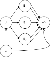
The floret of a vertex is defined as the sub-tree consisting of , its children, and the edges connecting its children (Freeman and Smith, 2011). Therefore, the idle factors of this graph are the 5 floret probability mass functions
| (7) |
respectively associated with the root vertex and the vertices labelled ,
Note that because it is saturated and contains no constraining structural information other than that logically entailed by the definition of its florets, must also hold for any intervened system too. Denote the corresponding floret probabilities in any intervened systems as
so that in particular ’s probability that they will detect the agent’s entry after will be
Denote ’s expected utility of doing nothing and doing by and respectively. It follows that
To calculate when the agent is unaware of the intervention , can use as an inferential framework for as well: using its implied factorisations and function and simply changing some of the factors within these formulae in the light of applying .
Thus in this setting the standard CEG inanimate causal rules (Thwaites et al., 2010) can be applied, where after the intervention we simply set and copy all other factors in the idle system. So in our notation set
implying ’s expected utility for enacting where denotes ’s probability of detecting an unaware agent after intervention . The CEG formula of the idle CEG using these new factors on then gives
and
So, as we might expect, if the new regime can be applied with no cost can safely conclude there is always a benefit in choosing the act over doing nothing , its efficacy being increasing in and and decreasing in : and its factorisation are sufficient for this causal analysis. Of course in practice the imposition of the new regime may well incur an additional cost, but the analysis above is easily adapted to take this into account - for example using standard multi-attribute utility analyses (Smith, 2010).
4 Intelligent Causal Algebras
4.1 Introduction
All the causal algebras discussed above implicitly assume that cannot react to a decision so as to soften its impact on them. However, such responses will be almost inevitable when modelling conflict or the sub-threshold. In this section, we describe how can systematically adapt an original model and embellish its topology into a new graph that is expressive enough to embed a transparent causal algebra that takes account of a single adversary’s potential reactions to ’s interventions. The original joint density associated with framework of the idle system is then simply a margin of the joint density framed around a more refined graph . We note that - in the context when is a BN - this concept that the idle system is observed as a margin of a more refined description that can then be exploited to examine inanimate cause is not new - it is in fact a central concept in determining whether or not a cause is identifiable (Pearl, 2000). Here we simply extend this concept so that it can be applied to other classes of graphical causal models for the particular contexts where we can expect a reaction to an intervention involving variables that are not directly observable from the idle system.
The method we propose to embed a model of ’s reactions builds on a now well established form of Bayesian game theory called Adversarial Risk Analysis (ARA) (Banks et al., 2015). Unlike more standard game theoretic approaches, following Kadane and Larkey (1982) and Smith (1996), within this genre of game theory, the roles of the two players and are not treated symmetrically. Instead the ARA model is built on behalf of just one player - here the defender . We show below that this approach harmonises well with the general type of graphical causal Bayesian analysis we have described above. It enables intelligent causal algebras - i.e. causal algebras where models what they believe will be ’s reaction to a when discovers it - in a way that is both feasibly realistic to the domain and formally justified.
The key to this embedding is for to assume a form of ARA analysis where assumes that is rational in the sense that they are a Subjective Expected Utility (SEU) maximiser. The defender can then put themselves in ’s shoes to double guess their responses. Two desirable features of a causal model (Hill, 1965) are that the underlying processes that it describes - here by the causal graph and its semantics - apply not only to the circumstances under study - here the idle system - but also other circumstances. In this adversarial setting we assume this is true for not only the different decisions that entertains, but also that other intelligent modelers share the same belief in the structure expressed by . A novel feature of this work is that it is argued below that - within this Bayesian setting - in choosing a causal as a framework of a causal algebra, should also strive to ensure that it is plausible that might use as a framework for their own reasoning as an SEU decision maker. We argue that when it is compelling for to do this, the graphical common knowledge shared by and can vastly simplify ’s inferences under an ARA analysis. This helps to scale up such methods to large problems and provide a transparent framework around which to explain, explore and adapt the ramifications of a given model.
In order to achieve this we argue that will often need to embellish their original causal structural framework expressed by into a new framework that is refined enough to explicitly model ’s potential reactions. A methodology for fleshing out into such a is described and then illustrated below.
4.1.1 A Risk Analysis Based on a Causal Graph
As Kadane and Larkey (1982) pointed out, from a Bayesian perspective, is free to choose a model of ’s rational reactions however they choose - in particular the types of rationality behind their reactions might employ. However, to develop a suitably generic methodology it is important to give guidance to about precisely how this might be done. We describe below some assumptions that if were to accept would enable them to systematically embed their beliefs of ’s intelligent reactions into their causal inferential framework.
We have argued above that if believes the underlying process is truly causal then there will exist a causal graph that can be used not only as a framework for ’s probability densities , but also ’s beliefs about what ’s beliefs might be.
Assumption 1: A Causal Common Knowledge Graph. ’s
beliefs about
can be framed by a causal graph , which believes
is also common knowledge (Hargreave-Heap and Varoufakis, 2004) to and .
Albeit outside a causal analysis, in previous studies of adversarial BN’s (Smith, 1996; Smith and Allard, 1996) and more recently for adversarial CEGs (Thwaites and Smith, 2017) it has been argued that for Assumption 1 to be compelling it must be plausible for to assume that will only use external information available to them when there is any advantage to them to do so. This enables to reason about ’s processing of structural information properties embedded in the semantics of the graphs we have explored here. In fact we have found that by making this assumption can sometimes reduce the complexity of a naively chosen graphical framework to a simpler one . We illustrate its use and state this assumption more explicitly below.
Assumption 2: Adversarial Parsimony. believes that whenever assigns the same expected utility score to two reactions , , where is an explicit function of a proper subset of the features of which is aware and on which is based, then will prefer to , .
In the types of adversarial settings we consider in this paper this is usually a compelling assumption because were not to do this then the additional complexity of ’s decision rules might then be exploited by - as discussed in Smith and Allard (1996) - in the context where is a BN. In this sense D believes that A will choose the most stable one out of the model perturbations of otherwise equivalent reactions.
Finally, and although not strictly necessary, we follow Banks et al. (2015) and recommend that once has assumed shares their own inferential framework , believes will assign the factors embellishing this graph as a boundedly rational player (Rios and Ríos Insua, 2012), here a 2 step thinker (Alderson et al., 2011). This enables to avoid the complexities of implications of an infinite regress concerning the factors might assign to their respective factors. In the context of the domains we address here this can be expressed as follows.
Assumption 3: A 2-step Adversarial Response. Whilst believes might well respond to what actually does, they believe will not try to act in a way to deceive in order to persuade to subsequently choose decisions that might be more advantageous to .
This assumption implicitly assumes that is one step ahead of : they take account of ’s reasoning as it will arise as a function of the decision that might commit to. However, in choosing their reaction believes will not choose its reactions based on their own beliefs about ’s beliefs beyond those encoded in the topology and colouring of the shared causal graph and its shared factors .
This is of course a substantive assumption and its applicability to any given adversarial domain always needs to be checked. For example, an adversary may well try to influence a defender by disguising their responsive capabilities and so deceive into choosing an erroneous decision more advantageous to . However, in settings like the one we describe in our running example, where ’s acts happen last and after will have committed to their action , it is almost automatic in the sense that ’s act can no longer influence ’s acts through such methods. However, in settings where decisions by and are simultaneous and sequential it can be a heroic assumption. An excellent discussion of these issues, beyond the scope of this paper, can be found in Stahl and Wilson (1994).
Embedding accepted dogma from game theory (Rios Insua et al., 2023), the new features that need to be imported by into so that a new graph can capture features about A which will determine their rational responses typically fall into the three categories below. Depending on the semantics of and , these typically can necessitate the introduction of additional vertices, edges and colourings into in ways we illustrate below. These three features are as follows:
-
1.
Whether or not, and if so when and which decisions discovers: represented by additional vertices labelled by .
-
2.
What believes ’s intents might be (Rios Insua et al., 2023). Within the Bayesian paradigm these are expressed in ’s specification of ’s utility function . For simplicity we assume that this intent is defined in a way that is fixed and invariant to whether no action is taken or whether any is chosen by . So, for example, variables in a BN describing are founder nodes and events associated with intent are near the root of a CEG describing the process.
-
3.
What of ’s resources, capabilities and MO/ playbook (Bunnin and Smith, 2020) might help determine how responds to frustrate ’s intervention - expressed by a vector of new variables . Note that in particular these will constrain the ways believes is capable of reacting - the space of their possible reactions : . Again, at least within any time slice this set too will be invariant to whether no action is taken or whether any is chosen by .
Once all the features of the problem in the three bullets above are in place, can then embed into how they believe might actually choose to react : these beliefs here represented by ’s random variable . The factors describing these acts are clearly in and need to be specified as part of the causal algebra for the particular type of application considered. There are three steps to construct an intelligent from an initial inanimate causal graph :
-
1.
Embellish the original unintelligent graphical model into an intelligent one in a way that is sufficiently refined to include all factors embedding the relevant features . This provides with a framework for reasoning about ’s (bounded) rationality.
-
2.
Evoke ’s rationality and parsimony to simplify into a final graph for ’s inferences about how might react to .
-
3.
Guide in how to choose appropriately the factors in D’s causal model for this graph with the quantitative forms of the factors - most challengingly those in - so that can calculate their own expected utility scores and hence evaluate the efficacy of each of their potential interventions.
This protocol is motivated by a rationale that is discussed in great detail in Banks et al. (2015). In summary - conditional on ’s utility function over ’s vector of attributes , their resources/capabilities/MO and what has learned about ’s chosen intervention under the assumptions above - will believe will choose a reaction to .
where
where is ’s density over the attributes of ’s utility.
Were able to perfectly predict , then because believes is an expected utility maximiser it follows that will believe ’s reaction is known to them for each contemplated intervention and triple . So can systematically construct the factors needed for their probability model by simply substituting this perfectly predictable reaction into their model of the process. They can then calculate their own expected utility maximising act . Note that when is uncertain about , can still predict their scores conditional on each value these variables can take and average over these to calculate their expected scores. Note that in this rational setting, since is perfectly predictable to , ’s reactions are deterministic functions of the states of this triple and so need not be included in the extended graph .
Of course, as pointed out in Banks et al. (2015) typically will be uncertain about the conditional probabilities that will integrate over to score the different options that will then determine how they act. However, our general causal framework provides a simpler setting to the more general setting described in Banks et al. (2015) when assumes that will share the same causal graph after enacts a decision . This then greatly simplifies ’s task to one of double guessing ’s factors that embellish this common knowledge graph . Although the elements in ’s set of factors - here denoted by - will typically be different from ’s corresponding factors in , they are usually relatively straightforward for to estimate. Thus, those associated with natural phenomena can plausibly conjecture they will be the same as their own. Furthermore, others will be degenerate. For example, by definition will know for sure and so their reactions So based on ’s beliefs about they are then able to determine a probability distribution over ’s reactions as a function of ’s factors. Note that the graph framing these inferences needs to be sufficiently detailed for to express their probabilistic beliefs about as this might apply to any .
The precise way in which these elements can be introduced into a graphical model obviously depend on the semantics of the graph framing the probability model as well as what and how believes might learn of their intervention. We illustrate below how it is possible to embellish a causal graph in this way using the simple incursion model, whose idle structure was given by the graph of the CEG given above.
4.2 An Incursion Model After a Rational Response
Constructing a New Graph to Model an Adversary’s Intelligence
Example 1 (Incursion continued).
Continuing the example above, assume that believes that might discover that had enacted once their agent is in place and ready to enter one of the ports. Strategic interest continues to be in determining the benefit of over doing nothing, .
From the discussion above needs to construct a more refined graph (see Fig. LABEL:fig:subfig2) than to model ’s intelligent reactions. Here we not only need to embed what believes might do in this setting, but also the choice represented by of which port his agent will try to slip through and also how he might react , framed by their capability once learning what had done (here ). Note in this example that the only features of ’s reaction relevant to are how might adapt their incursion plan - here either to abort their mission or switch their incursion attempt to ports or . This choice will depend on what believes ’s intent is - as expressed through ’s utility function and their capability to move from outside to one of the other ports. These new critical features are explicitly recognised in the graph . This introduces three new vertices and their emanating edges:
-
1.
A vertex denoted by whose emanating edges represent whether or not believes discovers ’s intervention after hearing this information when the agent has been transported to their planned port of entry.
-
2.
A vertex denoted by whose edges represent which port the agent might be positioned to enter when he hears about the intervention . Note that here assumes that will continue to enter or after hearing outside one of these ports.
-
3.
A vertex denoted by to represent the event that ’s agent is outside port when hearing about . Its emanating edges are directed into the port they intelligently react to switch their attempt to enter given this information. Notice the topology of the CEG asserts they will always switch to another port in this circumstance if at , or abort the attempted infiltration. There are 3 possible scenarios which challenge the agent’s capabilities - not capable of reaching either or , go to and go to . Each of these possible capabilities is expressed as an emanating edge from .
Here the newly introduced floret probabilities are - i.e. the emanating edge probabilities - rooted at the new vertex , the probability the agent hears about and floret probabilities rooted at new vertex , that the agent at chooses or is unable to complete the mission or that they switch to port from , respectively. The story line above ensures that the edge probabilities emanating from are the same as those emanating from since has assumed that could only learn that was put in place after had positioned their agent for entry - in CEG terminology and are in the same stage and given the same colour in the graph.
Thus, because and are in the same stage, there are now 7 embellishing probability factors of the new CEG emanating from for the idle system
Obviously in this case, since has not been enacted, . Note that have no effect on the atomic probabilities of this model using the composition formula of the CEG because they are always multiplied by zero. Therefore it is trivial to check that this gives the same formula for the idle system based on . In this sense the idle system described by is a margin of the idle system described by .
On the other hand, after the intervention , it is no longer certain that the now substantive intervention is discovered, so the edge probabilities emanating from the vertex are no longer . Therefore, the new set of factors can be partitioned into two sets where
where using Equation (6), it is easy to check that ’s probability of undetected incursion becomes
giving that
Note now that, in contrast to the case when cannot intelligently respond, it is no longer the case that should always prefer to : e.g. when and , would judge that it would be better not to intervene.
When performing this sort of extension the first step is to check whether it is indeed plausible for to assume that faithfully represents their own beliefs and what might believe. So suppose first that believes that has a utility function whose only attribute is an indicator on the event that ’s agent successfully infiltrates undetected. Then unusually is effectively completely known to . The same argument we used for ’s rationality would then lead to deduce that will then minimise their probability if their agent is detected.
Notice that, having made the assumption about ’s utility and that shares , can immediately deduce that will send the agent, otherwise ’s expected utility will be zero. So they can safely assume that . Therefore the graph - whilst valid - is over elaborate. It encourages to introduce unnecessary features into the analysis. The alternative simpler graph which omits is therefore appropriate
Here
and
The hypothesis that is SEU with a utility on the given attribute and that they share a causal graph has already modified ’s inferences.
Next, it is necessary to check whether it is plausible for to entertain a graphical model with the topology and colouring of the graph given they believe to be rational. Using the semantics of a CEG the structural assumptions implied by the graph , see Fig. LABEL:fig:subfig3.
-
1.
After a possible switch, given whether or not is enacted, the probability that the agent is caught is then unaltered.
-
2.
will only change their plans if their agent is positioned to enter port when he hears of .
-
3.
If this happens then will not attempt to enter , but enter either or or choose/be forced to abort the mission.
The first assumption is logically implied by ’s own beliefs about when might hear about . However, the remaining two relate to ’s beliefs about how will act. Suppose, believes that is a graph of what believes frames ’s probability model given their two possible decisions. Then the second assumption is automatic if assumes is parsimonious. For it is easy to check that whatever ’s factors, their expected utility would not increase through choosing a more complicated decision to change.
The third assumption again depends on ’s belief that shares . For example, if could infiltrate their agent through another port uncontemplated by then this assumption would clearly be violated. However, assume is confident that this is not the case. Then this assumption is valid were to believe that also believed that after the detection of the agent at port was certain. Then, for any reaction that included the agent attempting to infiltrate via for certain would ensure ’s expected utility . So unless thinks all other options are hopeless they will choose to try to enter either or
Given the topology of the graph is a valid framework for expressing ’s true beliefs about their attributes and ’s beliefs about these - as implied by common knowledge - it is sufficient for to consider the respective probabilities
will be sufficient to construct what believes ’s beliefs are. Although many of these will be known to , most will be uncertain to . However, believes that will try to maximise the value of their infiltrating undetected: i.e. maximise the function
A key point here is to notice that, through the definition of the variables in the problem, the only instrument has is to attempt to get to another port. This translates into choosing a reaction to maximise . The probabilities depend on ’s evaluation of arrival capability, which can place probabilities on but is unlikely to know precisely.
can now reason as follows. It would be plausible to to assume that - after all these are the current probabilities that can sample. Note that D here assume A shares their own factor. If D believes this then will choose to enter port either if is the only option, and A believes they cannot reach , or if A believes they can reach either alternative port and their odds Such an assessment would need to be based on ’s intelligence about ’s capabilities. This will need to be imported using information not needed in the idle system - for example information about the ease and the skills of the agent to travel between the ports. Nevertheless will have some information about this.
The probabilities then provides ’s odds that switches to and not , and these provide all the inputs needs to assess
and hence perform their strategic analysis under intelligent cause. Note here that all probabilities used in this equation could be elicited using standard techniques, protocols and code such as those presented in Williams et al. (2021). Of course, the analysis above is the simplest possible. Once we have the graphical model and its factors like this are in place we can, if necessary, bring in the usual Bayesian machinery to bring in our uncertainty about the parameters - using the usual suite of MCMC algorithms. Here this is ’s probabilistically expressed uncertainty about conditional probabilities factors (some of which are functions of ’s probabilities) and the latent triples . The causal algebra provides us with expected utility values conditional on each iteration of the MCMC algorithm. The implementation of such algorithms within standard ARA models is now well documented and so do not need to be discussed here. However, our point here is that the application of these algorithms greatly simplifies whenever a graphical causal algebra can be constructed that describes the process. Incidentally note that such algorithms can embed ’s beliefs that may not be fully rational, adding uncertainty to ’s rational choice - here to their selection of an alternative port when two might be possible.
4.2.1 Some Further Points Arising From This Example
It could be argued that could still be used by as a framework for inference in the example above. After all, subsequent to each intelligent , can be calculated as a margin of from which the effect margin after intervention could be calculated. However, then the derived interventional rules look mysterious. For example, after the intelligent reaction to the intervention above, the probabilities of an event happening preceding an intervention in the original graph of the idle system - there - will change. Furthermore, why and how these change is a function of information not embedded in the graph. So is not sufficiently refined to form any kind of systematic framework of a causal algebra and to capture the appropriate time line of events that affect what happens - whilst and are.
Next suppose, confronted with the analysis above, is still convinced it is possible that will abort their plan. Then the arguments above would force to conclude that either is not rational or more likely has misspecified ’s utility. The adversary’s preparedness would be entirely rational if assigns a positive utility to their agent not being caught. Thus, within their ARA, might conjecture that acts as if they have a multi-attribute utility where
where is an indicator on attribute - whether the agent successfully infiltrates as before - and is an indicator on attribute - an event of whether the agent is captured. The parameter , defines the criterion weights of this utility (Keeney and Raiffa, 1993; French and Rios Insua, 2010). It is straightforward now to rerun the analysis above when it can be checked that defined above, is in fact the appropriate framework to use and cannot be simplified. The associated equation is then constructed and explained.
Obviously the timing of when hears about an intervention is again critical and can influence the topology of the constructed graph. Finally, the necessary complexity of the graph used to extend is a function of the contemplated set of interventions . For example, suppose contemplates a larger space of functions that contains interventions to allocate extra resources at some proper subset of . If these interventions are in place, they will ensure the agent attempts to infiltrate that port - perhaps randomising across these options. would then need to embellish into containing new vertices that could describe what the agent would do when located outside one of the other ports on hearing information about the tightening of security within these other ports as well so that the efficacy of the new options could be tested. The graph is given in Fig. LABEL:fig:subfig4.
5 Dynamic Causal Graphs of an Intelligent Adversary
To demonstrate how such methods can scale up, we conclude this section by introducing a dynamic analogue of the example where an appropriate (now cyclic) graph the DCEG (Barclay et al., 2015) - analogous to a state space diagram of a semi-Markov process - has a slightly different semantic and the factor space is much larger. When a defender intervenes with beginning at a time , even when this intervention is initially covert, the subsequent unfolding of events together with any intelligence sources available to will mean that at future time points ’s intervention will be discovered by (at least partially). So any singular interventions that are planned to be enacted over several time steps will only remain covert until a given stopping time when discovers it. After such a stopping time, will then be able to act intelligently. So after that point we will need to apply the predictions that will embed their intelligent reaction using an appropriately crafted causal algebra.
Example 2 (Dynamic infiltration).
Assume that learns of a plan by to infiltrate no more than one agent on any day through ports and needs to quantify the efficacy of a decision to install the perfect detection system at port as discussed in the last example. Assume that ’s utility is linear in the number of agents they detect between day and day , . Assume that will not learn whether their agent’s infiltration will have been discovered before . The defender believes that - to make themselves as unpredictable as possible - ensures that the event they try to infiltrate an agent at one of the ports on any given day will be mutually independent, given the decision they take and whether or not the new system has been discovered by by that time .
A DCEG of this process is given in Fig. LABEL:fig:subfig5.
Because and are in the same stage there are factors/ stages associated with different floret probability vectors emanating from over the time slices. The factors of the idle system are now respectively
Under the intervention , in our notation
However, without additional external information there is no reason for to believe that will change their behaviour. So the probability vectors
will not depend on the time index . Note that in the dynamic setting it is possible that will have discovered and then reacts intelligently to this discovery. So now the probabilities are .
So must now specify , the probability that they will learn about the intervention at time , and , the probability they will abort at time , . The most naive model for assumes that ’s potential discovery would be totally random to them. Of course, logically, once has been discovered, it remains discovered. So then should set
Using the analogous arguments to the ones above it is possible to check that the graph is justified if assumes that has a utility function that is linear in the number of agents successfully infiltrating undetected.
With ’s assumed utility it is then easy to calculate that in this dynamic setting is
So the causal algebra gives us an explicit score for a strategic analysis in this new dynamic setting in terms of probabilities that can be linked directly to ’s beliefs of ’s thought processes - in ways analogous to those illustrated in the earlier simpler setting.
6 Discussion
In this paper, we have focused on developing a methodological framework for applying causal graphical inference in an adversarial setting. So we purposely illustrated the methodology with the simplest possible example that embodies the application of these ideas where a reactive adversary will try to frustrate the impacts of any defensive intervention. However, obviously our methods can also be applied to much more complex environments. So for example, complex causal analyses and protocols for adapted graphical forms of ARA are currently being examined for policing terrorist attacks orchestrated by hostile nations and for analyses of the possible exfiltration attacks (Bunnin and Smith, 2020; Shenvi et al., 2021). We note that in such cases bespoke graphical frameworks need to be developed that are demonstrably within the definition of a general class of causal graphical model given in this paper and where causal algebras also fully support the types of Bayesian strategic analyses needed in this setting. We defer the detailed discussion of these more domain specific causal graphical models to a later paper.
This paper has focused on how to set up prior models for adversarial decision making. Of course, the appropriate graphical model within a class could be learned using Bayesian model selection from data, either from analogous recorded cases or as a particular attack might be unfolding. In particular, when there is sufficient data available, a best explanatory graph , for example a BN, CEG or one of their dynamic analogues can be selected. The topologies and some of the conditional probability factors shared from the idle graph of the BN, CEG or alternative graphs can be learned using standard algorithms provided the data sets are rich enough.
However, when the intelligent reactions of an adversary need to be modelled it will hardly ever be the case that all the factors in can be learned from the idle system. Some will need to be imported from other data streams. Of course the usual Bayesian inferential framework and subsequent model selection is then ideal for guiding such selection. We nevertheless note that for at least some of the factors, because of their novelty or immediacy, will need to rely on elicited expert judgements to quantify their model. Again this is why Bayesian methods are especially valuable in these contexts where now well developed expert elicitation tools can be applied. Observe that because there are often systematically missing variables in the extended intelligent graph, many standard causal discovery tools will fail - although of course some causal conjectures can sometimes still be investigated for the BN graphical framework - when large complete observational data sets are available - using various routine methods like those discussed in Spirtes et al. (1993).
One current challenge is to develop bespoke elicitation methodologies for adversarial domains (Rios Insua et al., 2023). We find that directing thought experiments from ’s team about ’s likely reaction is a very delicate task both about the likely shared graph and the conditional probabilities that D should embellish this with, which properly take account of A’s likely reactions. The development for ARA elicitation is still in its infancy. However, we note that there are many such methods now developed for various graphical models (Cowell and Smith, 2014; Barons et al., 2018; Wilkerson and Smith, 2021; Korb and Nicholson, 2011) that could be developed to apply to adversarial models using the adversarial extensions of these models. The modularity the graphs induce make such elicitation easier than that needed more generically for ARA and appear to us a potentially very fruitful new area of research.
References
- Alderson et al. (2011) Alderson, D. L., Brown, G. G., Carlyle, W. M., and Wood, R. K. (2011). “Solving Defender-Attacker-Defender Models for Infrastructure Defense.” In Wood, R. K. and Dell, R. F. (eds.), Operations Research, Computing, and Homeland Defense, 28–49. Hanover, MD: INFORMS.
- Banks et al. (2015) Banks, D., Rios, J., and Ríos Insua, D. (2015). Adversarial Risk Analysis. Taylor & Francis.
- Barclay et al. (2015) Barclay, L., Collazo, R., Smith, J., Thwaites, P., and Nicholson, A. (2015). “Dynamic Chain Event Graphs.” Electronic Journal of Statistics, 9(2): 2130–2169.
- Barons et al. (2022) Barons, M., Fonseca, T., Davies, A., and Smith, J. Q. (2022). “An Integrating Decision Support System for Addressing Food Security in the UK.” The Royal Statistical Society Series A, 24.
- Barons et al. (2018) Barons, M., Wright, S., and Smith, J. (2018). “Eliciting Probabilistic Judgments for Integrating Decision Support Systems.” In Dias, L., Morton, A., and Quigley, J. (eds.), Elicitation: The Science and Art of Structuring Judgment, chapter 17, 445–478. Springer.
- Birkin and Wu (2012) Birkin, M. and Wu, B. (2012). “A Review of Microsimulation and Hybrid Agent-Based Approaches.” In Agent-Based Models of Geographical Systems, 51–68. Springer Netherlands.
- Bunnin and Smith (2020) Bunnin, F. and Smith, J. (2020). “A Bayesian Hierarchical Model for Criminal Investigations.” Bayesian Analysis. ArXiv:1907.01894.
- Collazo et al. (2018) Collazo, R., Gorgen, C., and Smith, J. (2018). Chain Event Graphs. Chapman & Hall.
- Cowell and Smith (2014) Cowell, R. G. and Smith, J. Q. (2014). “Causal discovery through MAP selection of stratified chain event graphs.” Electronic Journal of Statistics, 8: 965–997.
- Freeman and Smith (2011) Freeman, G. and Smith, J. (2011). “Bayesian MAP Selection of Chain Event Graphs.” Journal of Multivariate Analysis, 102: 1152–1165.
- French and Rios Insua (2010) French, S. and Rios Insua, D. (2010). Statistical Decision Theory: Kendall’s Library of Statistics 9. Probability & Mathematical Statistics.
- Hargreave-Heap and Varoufakis (2004) Hargreave-Heap, S. and Varoufakis, Y. (2004). Game Theory: A Critical Introduction. New York: Routledge.
- Hill (1965) Hill, A. B. (1965). “The Environment and Disease: Association or Causation?” Proceedings of the Royal Society of Medicine, 58(5): 295–300.
- Højsgaard and Lauritzen (2008) Højsgaard, S. and Lauritzen, S. L. (2008). “Graphical Gaussian models with edge and vertex symmetries.” Journal of the Royal Statistical Society: Series B (Statistical Methodology), 70(5): 1005–1027.
- Jaeger (2004) Jaeger, M. (2004). “Probability Decision Graphs – Combining Verification and AI Techniques for Probabilistic Inference.” International Journal of Uncertainty, Fuzziness, and Knowledge-based Systems, 12: 19–42.
- Kadane and Larkey (1982) Kadane, J. and Larkey, P. (1982). “Subjective Probability and the Theory of Games.” Management Science, 28(2): 113–120.
- Keeney and Raiffa (1993) Keeney, R. L. and Raiffa, H. (1993). Decisions with Multiple Objectives: Preferences and Value Tradeoffs. Cambridge: Cambridge University Press.
- Korb and Nicholson (2011) Korb, K. and Nicholson, A. (2011). Bayesian Artificial Intelligence. Chapman & Hall.
- Liverani and Smith (2016) Liverani, S. and Smith, J. Q. (2016). “Bayesian Selection of Graphical Regulatory Models.” International Journal of Approximate Reasoning, 77: 87–104.
- Naveiro et al. (2022) Naveiro, R., Insua, D. R., and Camacho, J. M. (2022). “Augmented probability simulation for adversarial risk analysis in general security games.” In Proceedings of the 12th International Defense and Homeland Security Simulation Workshop (DHSS), 18th International Multidisciplinary Modeling & Simulation Multiconference. Awarded with Best Paper Award.
- Pearl (2000) Pearl, J. (2000). Causality - Models, Reasoning and Inference. Cambridge University Press.
- Peters et al. (2016) Peters, J., Buhlmann, N., and Meinshaussen, N. (2016). “Causal Inference by using invariant prediction: identification and confidence intervals.” JRSSB, 78: 947–1012.
- Queen and Smith (1993) Queen, C. M. and Smith, J. Q. (1993). “Multiregression Dynamic Models.” Journal of the Royal Statistical Society Series B (Statistical Methodology), 55(4): 849–870.
- Rios and Ríos Insua (2012) Rios, J. and Ríos Insua, D. (2012). “Adversarial Risk Analysis for Counterterrorism Modeling.” Risk Analysis, 32: 894–915.
- Rios Insua et al. (2023) Rios Insua, D., Naveiro, R., Gallego, V., and Poulos, J. (2023). “Adversarial Machine Learning: Bayesian Perspectives.” Journal of the American Statistical Association, 1–22.
- Robins (1986) Robins, J. (1986). “A new approach to causal inference in mortality studies with a sustained exposure period—application to control of the healthy worker survivor effect.” Mathematical Modelling, 7(9–12): 1393–1512.
- Shafer (1996) Shafer, G. R. (1996). The Art of Causal Conjecture. Cambridge, MA: MIT Press.
- Shenvi et al. (2021) Shenvi, A., Bunnin, F., and Smith, J. (2021). “A Bayesian Decision Support System for Counteracting Activities of Terrorist Groups.” Math ArXiv.
- Smith (1996) Smith, J. (1996). “Plausible Bayesian Games.” In et al., B. (ed.), Bayesian Statistics 5, 551–560. Oxford University Press.
- Smith (2010) — (2010). Bayesian Decision Analysis: Principles and Practice. Cambridge University Press.
- Smith and Allard (1996) Smith, J. and Allard, C. (1996). “Rationality, Conditional Independence and Statistical Models of Competition.” Computational Learning and Probabilistic Reasoning, 237–256.
- Smith and Anderson (2008) Smith, J. and Anderson, P. (2008). “Conditional Independence and Chain Event Graphs.” Artificial Intelligence, 172(1): 42–68.
- Smith and Figueroa (2007) Smith, J. and Figueroa, L. (2007). “A Causal Algebra for Dynamic Flow Networks.” In Lucas, P., Gamez, J., and Salmeron, A. (eds.), Advances in Probabilistic Graphical Models, 39–54. Springer.
- Smith and Shenvi (2018) Smith, J. and Shenvi, A. (2018). “Assault Crime Dynamic Chain Event Graphs.” Technical report, Warwick Research Report (WRAP).
- Smith et al. (2015) Smith, J. Q., Barons, M. J., and Leonelli, M. (2015). “Decision focused inference on Networked Probabilistic Systems: with applications to food security.” In Proceedings of the Joint Statistical Meeting. Seattle.
- Spirtes et al. (1993) Spirtes, P., Glymour, C., and Scheines, R. (1993). Causation, Prediction and Search. New York: Springer.
- Stahl and Wilson (1994) Stahl, D. and Wilson, P. (1994). “Experimental Evidence on Players’ Models of Other Players.” Journal of Economic Behavior & Organization, 25: 309–327.
- Strong et al. (2022) Strong, P., McAlpine, A., and Smith, J. Q. (2022). “Towards A Bayesian Analysis of Migration Pathways using Chain Event Graphs of Agent Based Models.” In Proceedings of the Bayesian Young Statisticians Meeting (BaYSM).
- Thwaites and Smith (2017) Thwaites, P. and Smith, J. (2017). “A Graphical Method for Simplifying Bayesian Games.” Reliability Engineering and System Safety. Online: 12-MAY-2017, DOI: 10.1016/j.ress.2017.05.012.
- Thwaites et al. (2010) Thwaites, P., Smith, J., and Riccomagno, E. (2010). “Causal Analysis with Chain Event Graphs.” Artificial Intelligence, 174: 889–909.
- Wilkerson and Smith (2021) Wilkerson, R. and Smith, J. (2021). “Customised Structural Elicitation.” In Bedford, T., French, S., Hanea, A., and Nane, T. (eds.), Expert Judgment in Risk and Decision Analysis. Springer.
- Williams et al. (2021) Williams, C., Wilson, K., and Wilson, N. (2021). “A Comparison of Prior Elicitation Aggregation Using the Classical Method and SHELF.” Journal of the Royal Statistical Society Series A: Statistics in Society, 184.